Quantum error as an emergent magnetic field

Abstract

We investigate the effect of quantum errors on a monitored Brownian Sachdev-Ye-Kitaev (SYK) model featuring a measurement-induced phase transition that can be understood as a symmetry-breaking transition of an effective $Z_{4}$ magnet in the replica space. The errors describe the loss of information about the measurement outcomes and are applied during the non-unitary evolution or at the end of the evolution. In the former case, we find that this error can be mapped to an emergent magnetic field in the $Z_{4}$ magnet, and as a consequence, the symmetry is explicitly broken independent of the measurement rate. Rényi entropies computed by twisting boundary conditions now generate domain walls even in the would-be symmetric phase at a high measurement rate. The entropy is therefore volume-law irrespective of the measurement rate. In the latter case, the error-induced magnetic field only exists near the boundary of the magnet. Varying the magnetic field leads to a pinning transition of domain walls, corresponding to error threshold of the quantum code prepared by the non-unitary SYK dynamics.

Introduction.—Pure quantum states correspond to states of maximal knowledge of a quantum system, and various kinds of ideal quantum dynamics preserve this property, for example, unitary dynamics or projective measurements in which the complete measurement record is retained. Quantum errors occur when this idealized dynamics is interrupted, typically leading pure states to evolve into mixed states. Such errors are ubiquitous in nature and play a fundamental role across a variety of disciplines. For instance, in condensed-matter physics and quantum information physics, errors are inevitable because any realistic system in a lab is coupled to its environment, typically resulting in entangled states in which the system alone is no longer in a pure state.

In the emerging field of hybrid dynamics Li et al. (2018, 2019); Skinner et al. (2019); Choi et al. (2020); Gullans and Huse (2020a); Chan et al. (2019); Zabalo et al. (2020); Gullans and Huse (2020b); Li et al. (2020); Fan et al. (2020); Iaconis et al. (2020); Sang and Hsieh (2020); Lavasani et al. (2021); Ippoliti et al. (2021); Chen et al. (2020a); Alberton et al. (2020); Jian et al. (2020); Tang et al. (2021); Buchhold et al. (2021); Bao et al. (2021); Zhang et al. (2021a); Jian et al. (2021), it was recently discovered that the quantum trajectories resulting from chaotic unitary evolution and repeated measurements exhibit a phase transition between a volume-law and an area-law entangled phase Li et al. (2018, 2019); Skinner et al. (2019); Choi et al. (2020); Gullans and Huse (2020a). On one hand, failure to retain the complete measurement record for each quantum trajectory destroys this phase transition. In this case, the system is effectively coupled to an inaccessible environment, leading to a trivial thermal volume-law phase regardless of the coupling strength. On the other hand, strictly following the quantum trajectory, the hybrid circuit can be interpreted as preparing a quantum error correction code Choi et al. (2020); Gullans and Huse (2020a). In the context of error correction, the environment appears as an error that can cause the code to fail above a threshold Nielsen and Chuang (2001); Dennis et al. (2002).

In this paper, we develop a theoretical framework to understand the effects of quantum errors in non-unitary dynamics. Concretely, we use the monitored Brownian Sachdev-Ye-Kitaev (SYK) chain Jian et al. (2021); Kitaev (2015); Sachdev and Ye (1993); Maldacena and Stanford (2016); Liu et al. (2018); Gu et al. (2017); Huang et al. (2019); Zhang et al. (2020); Haldar et al. (2020); Zhang (2020); Chen et al. (2020b); García-García et al. (2021); Zhang et al. (2021b), and model quantum errors by throwing away individual measurement records with some probability. Without errors, the model exhibits a measurement-induced phase transition that can be understood as a symmetry-breaking transition of an effective $Z_{4}$ magnet in the replica space Jian et al. (2021). The subsystem entanglement entropy corresponds to the free energy of topological defects created by the twisted boundary conditions. In the symmetry-breaking phase at a low measurement rate, domains with different orientations are enforced by the twisted boundary condition and are separated by domain walls with finite line tension, giving rise to volume-law entanglement entropy. In the symmetric phase at a high measurement rate, the boundary condition can only change the free energy locally which leads to area-law entanglement entropy EE . We introduce errors in the non-unitary quantum dynamics (during the encoding process) or in the steady state (after the code is prepared), and analyze their effect on the entanglement scaling. In the former case, we find that quantum errors can be mapped to an emergent magnetic field in the $Z_{4}$ magnet. In the presence of such errors, the symmetry is explicitly broken independent of the measurement rate, and consequently, the measurement-induced phase transition is absent. In the latter case, the error induces a magnetic field near the boundary which leads to a pinning transition of domain walls. We argue that this is closely related to the error threshold problem for the quantum code generated by the non-unitary SYK dynamics. Notice that the connection between the pinning transition and the quantum error threshold has also been discussed in Refs. Li and Fisher, 2020; Gullans et al., 2020; Li et al., 2021. We also numerically calculate the subsystem entropy to show the absence of measurement-induced phase transition in the former, and the existence of the pinning transition in the latter.

Model and setup.— We consider the following Brownian SYK Hamiltonian of $L$ and $R$ chains Saad et al. (2018); Sünderhauf et al. (2019); Liu et al. (2020); Jian and Swingle (2020); Jian et al. (2021),

$$H=\sum_{x;a=L,R}\Big{(}\sum_{ij}iJ_{a,ij}^{x,x+1}(t)\psi_{x,a,i}\psi_{x+1,a,j}$$

$$+i^{q/2}\sum_{j_{1}<...<j_{q}}U_{a,j_{1}...j_{q}}^{x}(t)\psi_{x,a,j_{1}}...\psi_{x,a,j_{q}}\Big{)},$$ (1)

where $\psi_{x,a,i}$, $i=1,...,N$, denotes $i$-th of $N$ Majorana fermion at site $x$ of the $a\!=\!L,R$ chains. $L$ is the number of sites and periodic boundary conditions are assumed. The couplings $J_{a,ij}^{x,x+1}$ ($U_{a,j_{1},...,j_{q}}^{x}$) correspond to hopping (interaction) and are independent Gaussian variables with mean zero and variances

$$\overline{J_{a,ij}^{x,x+1}(t_{1})J_{a^{\prime},ij}^{x^{\prime},x^{\prime}+1}(t_{2})}=\frac{J}{2N}\delta(t_{12})\delta_{aa^{\prime}}\delta^{x,x^{\prime}},$$ (2)

$$\overline{U_{a,j_{1}...j_{q}}^{x}(t_{1})U_{a^{\prime},j_{1}...j_{q}}^{x^{\prime}}(t_{2})}=\frac{2^{q-2}(q-1)!U}{N^{q-1}}\delta(t_{12})\delta_{aa^{\prime}}\delta^{x,x^{\prime}}.$$

The system is under continuous monitoring given by measurement operators for the $i$-th Majorana fermion at site $x$ with probability $p$,

$$M_{1}=\kappa_{+}-\kappa_{-}\left(\frac{1}{2}+i\psi_{x,L,i}\psi_{x,R,i}\right),$$ (3)

$$M_{2}=s\left(\psi_{x,L,i}+i\psi_{x,R,i}\right),$$ (4)

where $\kappa_{\pm}\!=\!(\frac{1\pm\sqrt{1-4s^{2}}}{2})^{1/2}$, $0\!<\!s\!<\!\frac{1}{2}$ is the measurement strength, and $M_{1}^{\dagger}M_{1}+M_{2}^{\dagger}M_{2}=\mathbb{I}$. To model the error, we assume that when a measurement is performed, there is a probability $\gamma$ to lose the measurement record.

We are interested in calculating the quasi-$n$ entropy of bipartite system $A\bar{A}$ Napp et al. (2019),

$$S_{A}^{(n)}=\frac{1}{1-n}\log\frac{\mathbb{E}\text{Tr}(\rho_{A}^{n})}{\mathbb{E}\text{Tr}(\rho)^{n}}=\frac{1}{1-n}\log\frac{\mathbb{E}\text{Tr}(\rho^{\otimes n}X_{A})}{\mathbb{E}\text{Tr}(\rho^{\otimes n})},$$ (5)

where $\rho$ is the unnormalized density matrix, $X_{A}$ denotes the cyclic permutation acting on the subsystem $A$ of the $n$ replicated Hilbert space, and $\mathbb{E}$ denotes average over the Brownian and continuous monitoring evolution. We focus on the quasi-2 entropy, so we need four contours that are denoted as: $1,2$ ($3,4$) denote the first (second) replica, and $1,3$ ($2,4$) denote the forward (backward) evolution. When the measurement is implemented with a probability $p$, during a time step $\delta t$ the effective action in the four contours reads sup

$$(1-p)\mathbb{I}+p\sum_{i,j,\mu}w_{ij}^{(\mu)}M_{i}\otimes M_{i}^{\dagger}\otimes M_{j}\otimes M_{j}^{\dagger}$$ (6)

$$=\exp\delta t\Big{(}-\frac{\mu}{2}\sum_{\alpha}iG_{x,LR}^{\alpha\alpha}-\frac{\gamma\mu}{2}(M^{12}+M^{34})\Big{)},$$

where in the first line $w_{ij}^{(1)}\!=\!(1-\gamma)\delta_{ij}$ ($w_{ij}^{(2)}=\gamma$) corresponds to keeping (losing) the record. In the second line, $M^{\alpha\beta}\!=\!G_{LL}^{\alpha\beta}\!+\!G_{RR}^{\alpha\beta}\!-\!iG_{LR}^{\alpha\beta}\!+\!iG_{RL}^{\alpha\beta}$, $\alpha,\beta\!=\!1,...,4$ denote the four contours and $\mu=ps^{2}/\delta t$ is the measurement rate.

Including the Brownian Hamiltonian (Quantum error as an emergent magnetic field) and the measurement (S5) and integrating out the Gaussian variables, the effective action is

$$\!-\!\frac{I}{N}=\frac{1}{2}\text{Tr}\log[(-1)^{\alpha+1}\delta^{\alpha\beta}\delta_{ab}\partial_{t}\!-\!\Sigma_{ab,x}^{\alpha\beta}]-\frac{1}{2}\int\Sigma_{ab,x}^{\alpha\beta}G_{ab,x}^{\alpha\beta}$$

$$\!+\!\int\delta(t\!-\!t^{\prime})\Big{[}\frac{(-1)^{\alpha+\beta+1}}{4}\delta_{ab}[JG_{ab,x}^{\alpha\beta}G_{ab,x+1}^{\alpha\beta}+\frac{U}{2q}(2G_{ab,x}^{\alpha\beta})^{q}]$$

$$-\frac{\mu}{2}\sum_{\alpha}iG_{x,LR}^{\alpha\alpha}-\frac{\gamma\mu}{2}(M^{12}+M^{34})\Big{]}.$$ (7)

where $\Sigma_{ab,x}^{\alpha\beta}(t,t^{\prime})$ is the self energy introduced to enforce $G_{ab,x}^{\alpha\beta}(t,t^{\prime})=\frac{1}{N}\sum_{j}\psi_{x,a,j}^{\alpha}(t)\psi_{x,b,j}^{\beta}(t^{\prime})$. The summations over $x$, $a,b$ and $\alpha,\beta$ are implicit. We focus on $q=4$.

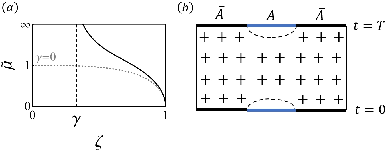
Figure 1: (a) An illustration of $\zeta$ determined by $\tilde{\mu}$ in (9). When $\gamma>0$, one can see that $\zeta>\gamma$. The case for $\gamma=0$ is plotted by the dotted line for comparison. (b) A schematic plot of domain wall configurations. Throughout the paper, the $+$ and $-$ indicates $(\phi_{1}\!>\!0,\phi_{2}\!=\!0)$ and $(\phi_{1}\!=\!0,\phi_{2}\!>\!0)$, respectively, and the black (blue) thick line denotes the boundary pointing toward $+$ ($-$) at boundaries $t=0$ and $T$. The magnetic field points toward $+$ direction.

Emergent magnetic field.— The saddle-point solution to the large-$N$ action within a replica reads

$$\bar{G}=\frac{e^{-\frac{|t|}{2}(J+U\zeta^{2}+\frac{\gamma\mu}{\zeta})}}{2}[\text{sgn}(t)\sigma^{z}-\zeta i\sigma^{y}-\frac{\mu\tau^{y}(1+\gamma\sigma^{x})}{J+U\zeta^{2}+\mu\frac{\gamma}{\zeta}}],$$ (8)

where Pauli matrix $\sigma$ ($\tau$) acts on 1 and 2 contours ($L$ and $R$ chains). The solution on $3,4$ contours is the same, consistent with the boundary condition without twist operators. The parameter $\zeta$ is given via the relation,

$$\tilde{\mu}=\frac{\zeta(1+\tilde{U}\zeta^{2})[\gamma(1-\zeta^{2})+\zeta\sqrt{(1-\zeta^{2})(1-\gamma^{2})}]}{\zeta^{2}-\gamma^{2}},$$ (9)

with $\tilde{U}\!=\!\frac{U}{J}$ and $\tilde{\mu}\!=\!\frac{\mu}{J}$.

When $\gamma\!=\!0$, (Quantum error as an emergent magnetic field) has $C_{4}\!\times\!C_{4}$ symmetry Jian et al. (2021), $G_{ab,x}\rightarrow O^{-1}G_{ab,x}O,$ where $O=e^{i(\theta_{13}\gamma_{13}+\theta_{13}\theta_{24})}$ acts identically on the left and right chains. $\gamma_{ij}^{\alpha\beta}\!=\!\delta_{i}^{\alpha}\delta_{j}^{\beta}-\delta_{j}^{\alpha}\delta_{i}^{\beta}$, and $\theta_{13},\theta_{24}=\frac{n\pi}{2}$ ($n$ is an integer). The relative rotation symmetry generated by $\gamma_{13}-\gamma_{24}$ is spontaneously broken by nonzero $\zeta$ in solution (8). If no error occurs, i.e., $\gamma\!=\!0$, (9) reproduces the measurement-induced phase transition in Ref. Jian et al., 2021, where $\zeta\!>\!0$ for $\tilde{\mu}\!<\!1$ corresponds to a symmetry-breaking phase with volume-law entanglement and $\zeta\!=\!0$ for $\tilde{\mu}\!\geq\!1$ corresponds to a symmetric phase with area-law entanglement. The transition can be understood as symmetry restoration due to the strong measurement $\mu\!>\!J$. However, in the presence of the record loss error $\gamma\!>\!0$, the relative $C_{4}$ symmetry in (Quantum error as an emergent magnetic field) is explicitly broken. Moreover, one can see that $\zeta\!>\!\gamma$ for all values of $\tilde{\mu}$ as illustrated in Fig. 1(a). Even at strong measurement $\tilde{\mu}\gg 1$, we have $\zeta\!\approx\!\gamma[1\!+\!\frac{(1-\gamma)(1+\tilde{U}\gamma^{2})}{\tilde{\mu}}]\!>\!\gamma$. It indicates that the symmetry breaking transition is absent for nonzero errors.

We can proceed to evaluate the effective theory by treating $\gamma$ perturbatively. In terms of $\phi_{1}\!=\!\delta G^{12}\!+\!\delta G^{34}$ and $\phi_{2}\!=\!\delta G^{14}\!+\!\delta G^{23}$ LR that transforms as a vector $\vec{\phi}\!\equiv\!(\phi_{1},\phi_{2})$ under $C_{4}$ rotation, i.e., $\phi_{1}\!\rightarrow\!-\phi_{2}$, $\phi_{2}\!\rightarrow\!\phi_{1}$, the effective theory reads sup

$$\frac{I_{\text{eff}}}{N}=\frac{1}{2}\sum_{k}\int_{\Omega}\left(\frac{\Omega^{2}}{\mu}+J(1-\cos k)\right)|\vec{\phi}_{k}(\Omega)|^{2}$$

$$+\sum_{x}\int_{t}\left(\frac{\mu-J}{2}\vec{\phi}_{x}^{2}+\frac{\gamma\mu}{2}\phi_{1}+\frac{\mu}{8}\vec{\phi}_{x}^{4}-\frac{U}{4}(\phi_{1,x}^{4}+\phi_{2,x}^{4})\right).$$ (10)

where $\int_{\Omega}\!=\!\int\frac{d\Omega}{2\pi}$, $\int_{t}\!=\!\int dt$, and $\vec{\phi}_{k}\!=\!\frac{1}{\sqrt{L}}\sum_{x}\vec{\phi}_{x}e^{-ikx}$. It is apparent that $\gamma$ behaves like a magnetic field along $\phi_{1}$ direction, and breaks $C_{4}$ rotational symmetry explicitly.

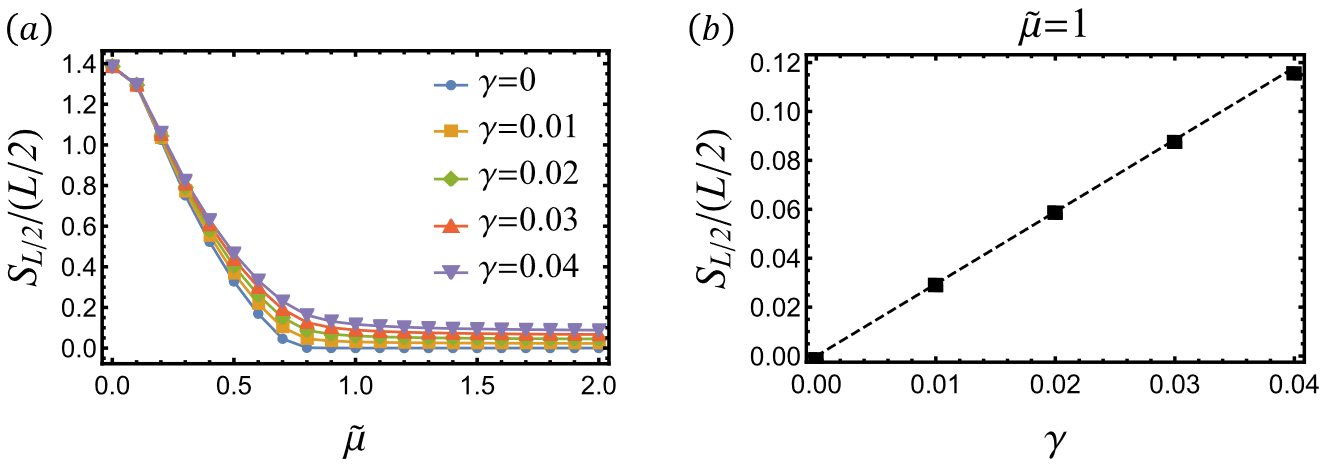
Figure 2: (a) The half-chain quasi entropy density of the steady state with and without record loss. (b) The entropy density at $\tilde{\mu}=1$ is linear in $\gamma$. Here we take $\tilde{U}=0.4$, and to get the density we make a linear fit for sites $L=12,14,16,18$, and $TJ=L$.

Absence of measurement-induced phase transition.— As shown in Ref. Jian et al., 2021, the swap operator in (5) amounts to changing the boundary condition of the vector field $\vec{\phi}$ in the subsystem $A$, and the quasi entropy corresponds to the free energy difference between configurations with and without the change of the boundary condition. To be concrete, we start from the thermofield double state (TFD) in the doubled Hilbert space Gu et al. (2017); Penington et al. (2019); Chen et al. (2020b); Jian et al. (2021) and divide the systems into two parts $A$ and $\bar{A}$. The quasi entropy at time $T/2$ is obtained by imposing twist operators at time $t\!=\!0$ and $t\!=\!T$ in the subsystem $A$, which require the boundary of $A$ has $(\phi_{1}\!=\!0,\phi_{2}\!>\!0)$ whereas that of $\bar{A}$ has $(\phi_{1}\!>\!0,\phi_{2}\!=\!0)$. If the $C_{4}$ symmetry is broken by nonzero magnetic orders, the boundary condition will lead to different domains and will also induce the domain walls between them, as illustrated in Fig. 1(b).

For simplicity, we redefine the theory (S18) to be

$$\frac{I_{\text{eff}}}{N}\!=\!\int dtdx[\frac{1}{2}(\partial\vec{\phi})^{2}+h\phi_{1}+r\vec{\phi}^{2}+\lambda\vec{\phi}^{4}+\lambda^{\prime}\left(\phi_{1}^{4}+\phi_{2}^{4}\right)],$$

with $r\!=\!\frac{\mu(\mu-J)}{2}$, $\lambda\!=\!\frac{\mu^{5/2}}{4\sqrt{2J}}$, $\lambda^{\prime}\!=\!-\!2\tilde{U}\lambda$ and $h\!=\!\gamma\frac{\mu^{7/4}J^{1/4}}{2^{5/4}}$. At the leading order, the free energy difference is given by the domain walls cost, $S_{A}^{(2)}=2N\sigma L_{A}$, where line tension can be obtained perturbatively for $r\leq 0$,

$$\sigma \approx\frac{\pi\sqrt{-\lambda^{\prime}}}{8}(\frac{-r}{\lambda+\lambda^{\prime}})^{3/2}+\frac{\pi-2}{(-2\lambda^{\prime})^{1/2}}h.$$ (11)

The first term reproduces the line tension without errors in the measurement-induced phase transition Jian et al. (2021), and the second term is independent of the tuning parameter $r$, which implies at $r\!=\!0$ the quasi entropy is still volume-law. On the other hand, for $r\!\gg\!0$, because the magnetic order pinned by the magnetic field points along $\phi_{1}$ direction in the bulk and pinned by the boundary condition points along $\phi_{2}$ direction at the boundary of subsystem $A$, they create a domain wall near the boundary with thickness given by the correlation length $\xi\!\propto\!r^{-1/2}$. Thus, the free energy cost is again linear in the subsystem length, i.e., $S_{A}^{(2)}\!\propto\!Nhr^{-1/2}L_{A}$, and the quasi entropy is volume-law for $r\!>\!0$.

In summary, the line tension is finite when $h\!>\!0$ and changes smoothly as a function of $r\!\propto\!\tilde{\mu}\!-\!1$, so the measurement-induced phase transition is absent in the presence of quantum errors. We confirm this conclusion with numerical results for the steady state quasi entropy density shown in Fig. 2. Fig. 2(a) shows that the transition disappears when $\gamma\!>\!0$ because the entropy density is finite for all $\tilde{\mu}$. Fig. 2(b) confirms the quasi entropy density at $\tilde{\mu}\!=\!1$ is linear in $\gamma$.

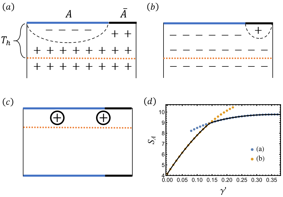
Figure 3: Two types of domain walls (a) and (b) in the presence of magnetic field near the boundary. The magnetic field points toward $+$ direction. The orange dashed line is the boundary of the region with magnetic field, i.e., $T\!<\!t\!<\!T\!+\!T_{h}$. (c) shows the boundary condition and the magnetic field near the top boundary in the quasi entropy $S_{A}^{(2)}$ calculated in (d). The “$+$” sign in the circle indicates the direction of the magnetic field. (d) The pinning transition of the subsystem quasi entropy of $L_{A}/L=2/3$ with $L=24$, $TJ=12$, $\tilde{\mu}=0.6$, and $\tilde{U}=0.4$. The entropy corresponding to type $(a)$ and $(b)$ are shown by the different colors.

Pinning of domain walls.— In an ordered magnet, the presence of an external magnetic field near the boundary can induce a first-order pinning transition of magnetic domains pin . Consider the case where a field pointing toward the direction of $\phi_{1}$ (the “$+$” direction) exists in a region of width $T_{h}$ near the top boundary (i.e. the region $T\!<\!t\!<\!T\!+\!T_{h}\!$) with a “$+$” boundary condition $(\phi_{1}\!=\!0,\phi_{2}\!>\!0)$ for subsystem $\bar{A}$ and a “$-$” boundary condition $(\phi_{1}\!>\!0,\phi_{2}\!=\!0)$ for subsystem $A$. Note that $T_{h}$ is kept fixed when the thermodynamic limit is taken $JT\sim L\rightarrow\infty$. Two types of domain walls are possible, one enclosing subsystem $A$ and the other $\bar{A}$ as shown in Fig. 3(a) and (b), respectively. Since the magnetic field favors the “$+$” direction, it pushes the domain wall in Fig. 3(a) away from the bulk but pulls the domain wall in Fig. 3(b) into the bulk. To leading order, the free energies of Fig. 3(a) and Fig. 3(b) are given respectively by sup

$$F_{a}(x)=N\sigma x,\quad F_{b}(x)=N\sigma x-NhT_{h}x.$$ (12)

where $x$ is the distance between the end points of domain walls at the boundary, and $\sigma$ ($h$) is the line tension (the magnetic field strength).

Below we assume $L_{A}\!>\!L_{\bar{A}}$ to observe a pinning transition. At zero magnetic field, the configuration of Fig. 3(b) dominates over that of Fig. 3(a) because $L_{A}\!>\!L_{\bar{A}}$. As the magnetic field increases, a pinning transition occurs when the two configurations have comparable free energies: $F_{a}(L_{A})=F_{b}(L_{\bar{A}})+NhT_{h}L$, where in addition to the domain wall free energy in (12) the energy cost of the disfavored domain in Fig. 3(b) must be taken into account on the right-hand side. This gives the transition point $h^{\ast}=\frac{2a-1}{a}\frac{\sigma}{T_{h}}$ ($a\!=\!\frac{L_{A}}{L}$), above which the dominant configuration switches to Fig. 3(a). Notice that in this calculation, we have implicitly assumed that the configurations in $0\!<\!t\!<\!T\!$ are the same.

In the following, we also consider other domain walls near $t\!=\!0$ boundary. This only leads to a shift in the critical field for the pinning transition. The first-order pinning transition is manifest in the quasi entropy $S_{A}^{(2)}$ of the steady state (with initial state being TFD), where the corresponding boundary condition and emergent magnetic field are shown in Fig. 3(c). Note that in this case the record loss occurs only near the boundary with a probability denoted by $\gamma^{\prime}$ to distinguish from $\gamma$ which is used for the record loss throughout the circuit in the previous section. In the language of encoding introduced in next section, $\gamma$ ($\gamma^{\prime}$) corresponds to record loss errors during (after) the encoding procedure. A pinning transition between the two domain wall configurations occurs as one increases the probability $\gamma^{\prime}$ as shown in Fig. 3(d).

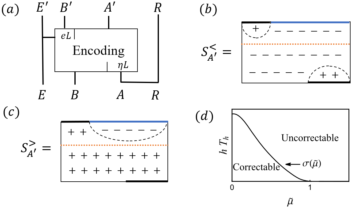
Figure 4: (a) Encoding process and possible quantum errors. See the main text for a detailed description. (b,c) Domain wall configurations corresponding to $S_{A^{\prime}}^{(2)}$ before and after the pinning transition. The orange dashed line is the boundary of the region with magnetic field, i.e., $T\!<\!t\!<\!T\!+\!T_{h}$. (d) The error correction transition is given by the line tension without record loss. The correction to the line tension from the error is neglected.

Quantum error correction.— The hybrid circuit can be understood as a quantum channel to generate an error correcting code for protecting quantum information Choi et al. (2020); Gullans and Huse (2020a); Li and Fisher (2020); Li et al. (2021). A schematic plot of the encoding process and possible quantum errors are shown in Fig. 4(a). To encode the information, one embeds it in region $A$ of the chain $|A|\!=\!\eta L$. By introducing a reference $R$, the initial state is given by a pure state in $AR$ tensor product with $B$, i.e., $\rho=\rho_{B}\otimes|\psi_{AR}\rangle\langle\psi_{AR}|$. Applying a circuit of depth $T$ generates a code, $\mathcal{E}(\rho)\!=\!\frac{C_{L}\rho C_{L}^{\dagger}}{\sqrt{\text{Tr}(C_{L}^{\dagger}C_{L}\rho)}}$, where $C_{L}$ denotes the circuit that acts on the system $AB$ but not on the reference $R$. Here, besides record loss, we also consider erasure errors that are commonly studied in the literature Gullans et al. (2020): the erasure error occurs in the region $B^{\prime}$ of the chain $|B^{\prime}|\!=\!eL$ at the boundary $t\!=\!T\!+\!T_{h}$. This is to be compared with the record loss, which occurs with a probability $\gamma^{\prime}$ near the boundary in the strip $[T\!,T\!+\!T_{h}]$. Notice that both errors happen at $t>T$ and we assume the encoding procedure is perfect in $0\!<\!t\!<\!T$. It is useful to model the record loss as a coupling to an environment $E$. Because we cannot access the information in region $E^{\prime}B^{\prime}$, the mutual information $I(R;E^{\prime}B^{\prime})\!=\!S_{R}\!+\!S_{E^{\prime}B^{\prime}}\!-\!S_{E^{\prime}B^{\prime}R}$ measures the information diminished by errors Schumacher and Nielsen (1996). If $I(R;E^{\prime}B^{\prime})\!=\!0$, it implies that the information is not lost and can be perfectly decoded.

At zero measurement rate, because the Brownian unitary dynamics can reach 2-design Onorati et al. (2017); Brandão et al. (2019); fra in polynomial time, the decoupling theorem Abeyesinghe et al. (2009) applies and predicts the error threshold to be $1\!-\!2e_{c}\!-\!\eta\!=\!0$. It turns out the domain wall picture can reproduce the same result at zero measurement rate. For finite measurement rate, although the decoupling theorem is not applicable, the domain wall picture and the associated pinning transition persist and provide an estimate of the quantum error threshold via the quasi-2 entropy. We assume the domain wall picture still holds for the von Neumann entropy and leave its verification for future study.

By introducing the environment $E$, the total pure wave function at time $T$ consists of four parts, $E^{\prime},B^{\prime},A^{\prime}$ and $R$, so $S_{E^{\prime}B^{\prime}R}^{(2)}=S_{A^{\prime}}^{(2)}$. Fig. 4(b) and (c) show the configurations before and after the pinning transition in $S^{(2)}_{A^{\prime}}$ respectively. Considering these two configurations, the entropy is

$$S^{(2)}_{A^{\prime}}=-\log(e^{-F_{a}((1-e)L)}+e^{-[F_{b}(eL)+NhT_{h}L]}e^{-N\sigma\eta L}).$$

In the second term inside the logarithm, the domain wall for the reference $R$ is included. [See Fig. 4(b), where we have a domain wall ending at $t\!=\!0$ boundary.] The above equation determines the erasure error threshold $e_{c}$ in the presence of the record loss,

$$hT_{h}(1-e_{c})=\sigma(1-2e_{c}-\eta).$$ (13)

Equivalently, if the erased portion is fixed, the transition is precisely the pinning transition at $h^{\ast}=\frac{1-2e-\eta}{1-e}\frac{\sigma}{T_{h}}$.

It is worth noting that there is also a similar pinning transition in $S_{E^{\prime}B^{\prime}}^{(2)}$. Including pinning transitions in both $S_{A^{\prime}}^{(2)}$ and $S_{E^{\prime}B^{\prime}}^{(2)}$, the mutual information reads

$$I^{(2)}(R;E^{\prime}B^{\prime})=$$

$$\qquad\qquad\begin{cases}0&e\!<\!e_{c}\\ N[\sigma(\eta+2e-1)+hT_{h}(1-e)]L&e_{c}\!<\!e\!<e_{*}\\ 2N\sigma\eta L&e_{*}\!<\!e\end{cases},$$

where $e_{\ast}$ given by $hT_{h}(1-e_{\ast})\!=\!\sigma(1\!-\!2e_{\ast}\!+\!\eta)$ is from the pinning transition in $S_{E^{\prime}R^{\prime}}^{(2)}$. If no erasure error occurs, $\sigma\!=\!hT_{h}$ according to (13), which indicates an error correction transition due to the record loss. Neglecting the correction to the line tension from the magnetic field when the record loss error is small, the threshold is then determined by the line tension in zero magnetic field as shown in Fig. 4(d).

Concluding remarks.— To conclude, with a concrete solvable model we show that the record loss error effectively generates a coupling between two Keldysh contours within each replica. Such a coupling explicitly breaks the permutation symmetry among the forward (backward) contours in different replica. We expect this result to be valid in more general errors because tracing out an environment that is coupled to the system will generate the inter-Keldysh coupling within each replica.

Remarkably, the domain wall picture of quantum error correction can also be generalized to the Hayden-Preskill protocol Hayden and Preskill (2007), where the information of part $B$ is collected before the encoding process. This can be interpreted as the collected Hawking radiation from the early black hole. A direct application of the domain wall picture leads to the error threshold $hT_{h}(1-e)\!=\!2\sigma(1-e-\eta)$ sup . It would be interesting to explore the effect of the quantum error on the decoding process Yoshida and Kitaev (2017).

Acknowledgement.— SKJ and BGS are supported by the Simons Foundation via the It From Qubit Collaboration. The work of BGS is also supported in part by the AFOSR under grant number FA9550-19-1-0360. PZ acknowledges support from the Walter Burke Institute for Theoretical Physics at Caltech. CL is supported by the NSF CMMT program under Grants No. DMR-1818533. We acknowledge the University of Maryland High Performance Computing Cluster (HPCC).

I Supplemental Material for “Quantum error as an emergent magnetic field”

II Derivation of the large-$N$ action and the saddle-point equation of the monitored system

The derivation of the large-$N$ action of the Brownian SYK model is a standard one Saad et al. (2018), so we focus on the effect of the measurement. As mentioned in the main text, the system is under continuously monitoring given by the measurement operators for the $i$-th Majorana fermion of left and right chains at site $x$,

$$\{M_{1},M_{2}\}=\left\{\Big{(}\frac{1+\sqrt{1-4s^{2}}}{2}\Big{)}^{1/2}-\Big{(}\frac{1-\sqrt{1-4s^{2}}}{2}\Big{)}^{1/2}\left(\frac{1}{2}+i\psi_{x,L,i}\psi_{x,R,i}\right),s\left(\psi_{x,L,i}+i\psi_{x,R,i}\right)\right\},$$ (S1)

where $0<s<\frac{1}{2}$ is the strength of measurement. During a time step, the measurement with a probability $p$ leads to the following operator for the two replicas,

$$(1-p)\mathbb{I}+p(1-\gamma)\sum_{i}M_{i}\otimes M_{i}^{\dagger}\otimes M_{i}\otimes M_{i}^{\dagger}+p\gamma\sum_{i}M_{i}\otimes M_{i}^{\dagger}\otimes\sum_{j}M_{j}\otimes M_{j}^{\dagger}$$ (S2)

$$=1-p+p(1-\gamma)\Big{(}1-s^{2}\sum_{\alpha=1}^{4}(\frac{1}{2}+i\psi_{x,L,i}^{\alpha}\psi_{x,R,i}^{\alpha})\Big{)}+p\gamma K_{43}K_{21},$$ (S3)

where $K_{kl}$ in the second line is defined as

$$K_{kl}=1-s^{2}\sum_{\alpha=k}^{l}(\frac{1}{2}+i\psi_{x,L,i}^{\alpha}\psi_{x,R,i}^{\alpha})+s^{2}(\psi_{x,L,i}^{k}\psi_{x,L,i}^{l}+\psi_{x,R,i}^{k}\psi_{x,R,i}^{l}-i\psi_{x,L,i}^{k}\psi_{x,R,i}^{l}+i\psi_{x,R,i}^{k}\psi_{x,L,i}^{l}).$$ (S4)

and the derivation is kept up to the $O(s^{2})$ order. $\gamma$ is the probability of losing the measurement outcome when a measurement is implemented. We perform the measurement for every Majorana species $i$ at every site $x$, and the result is the following effective action

$$\exp\delta t\left(-\frac{\mu}{2}\sum_{\alpha}iG_{x,LR}^{\alpha\alpha}-\frac{\gamma\mu}{2}\big{[}M^{12}+M^{34}\big{]}\right).$$ (S5)

where $M^{\alpha\beta}=G_{LL}^{\alpha\beta}+G_{RR}^{\alpha\beta}-iG_{LR}^{\alpha\beta}+iG_{RL}^{\alpha\beta}$, and $\mu=ps^{2}/\delta t$ is the measurement rate. This is (6) in the main text. Integrating out the Gaussian variables, the large-$N$ action is

$$-\frac{I}{N} = \frac{1}{2}\text{Tr}\log\left((-1)^{\alpha+1}\delta^{\alpha\beta}\delta_{ab}\partial_{t}-\Sigma_{ab,x}^{\alpha\beta}\right)+\iint-\frac{1}{2}\Sigma_{ab,x}^{\alpha\beta}(t,t^{\prime})G_{ab,x}^{\alpha\beta}(t,t^{\prime})$$ (S6)

$$+\iint\delta(t-t^{\prime})\Big{[}-\frac{(-1)^{\alpha+\beta}}{4}\delta_{ab}\left(JG_{ab,x}^{\alpha\beta}G_{ab,x+1}^{\alpha\beta}+\frac{U}{2q}(2G_{ab,x}^{\alpha\beta})^{q}\right)$$

$$-\frac{\mu}{2}\sum_{\alpha}iG_{x,LR}^{\alpha\alpha}-\frac{\gamma\mu}{2}\big{[}M^{12}+M^{34}\big{]}\Big{]},$$

where $\alpha,\beta=1,...,4$ denote the four contours. The summations over $x$, $a,b$ and $\alpha,\beta$ are implicit. $\Sigma_{ab,x}^{\alpha\beta}(t,t^{\prime})$ is the self-energy field introduced to enforce $G_{ab,x}^{\alpha\beta}(t,t^{\prime})=\frac{1}{N}\sum_{j}\psi_{x,a,j}^{\alpha}(t)\psi_{x,b,j}^{\beta}(t^{\prime})$. The saddle point equation reads

$$[G_{x}^{-1}]^{\alpha\beta}_{ab} = (-1)^{\alpha+1}\delta^{\alpha\beta}\delta_{ab}\partial_{t}-\Sigma_{ab,x}^{\alpha\beta},$$ (S7)

$$\Sigma_{ab,x}^{\alpha\beta}(t,t^{\prime}) = \delta(t-t^{\prime})\Big{[}\frac{-(-1)^{\alpha+\beta}\delta_{ab}}{2}\left(J(G_{ab,x-1}^{\alpha\beta}+G_{ab,x+1}^{\alpha\beta})+U(2G_{ab,x}^{\alpha\beta})^{q-1}\right)$$ (S8)

$$-i\frac{\mu}{2}\bar{\delta}_{LR}^{\alpha\alpha}-\big{(}\frac{\gamma\mu}{2}\bar{\delta}_{aa}^{12}-i\frac{\gamma\mu}{2}(\bar{\delta}_{LR}^{12}-\bar{\delta}_{RL}^{12})+\frac{\gamma\mu}{2}\bar{\delta}_{aa}^{34}-i\frac{\gamma\mu}{2}(\bar{\delta}_{LR}^{34}-\bar{\delta}_{RL}^{34})\big{)}\Big{]}.$$

where we define a short-hand notation $\bar{\delta}_{cd}^{\gamma\delta}\equiv\delta^{ac}\delta^{bd}\delta_{\alpha\gamma}\delta_{\beta\delta}-\delta^{bc}\delta^{ad}\delta_{\beta\gamma}\delta_{\alpha\delta}$.

III Derivation of the effective action (10)

We proceed to look at the effective theory by treating $\gamma$ perturbatively. Without the magnetic field, the symmetric solution reads

$$\bar{G}(t_{1},t_{2}) = \frac{e^{-\frac{\mu}{2}|t_{12}|}}{2}\left(\begin{array}[]{cccc}\text{sgn}(t_{12})&0&i&0\\ 0&-\text{sgn}(t_{12})&0&i\\ -i&0&\text{sgn}(t_{12})&0\\ 0&-i&0&-\text{sgn}(t_{12})\end{array}\right).$$ (S13)

where the basis of the matrix is $(L1,L2,R1,R2)$. And the solution is the same for contour $3$ and $4$. We consider the fluctuation away from the symmetric saddle-point solution (S13), so that the effect of the record loss is reflected in the effective action. The kernel of $\delta\Sigma$ from expanding the trace log term can again be brought into decoupled sectors, and because they serve as an order parameter we focus on the components $(\delta\Sigma^{12}_{aa},\delta\Sigma^{34}_{aa},\delta\Sigma^{14}_{aa},\delta\Sigma^{23}_{aa})$ whose kernel is given by

$$K=\frac{\mu}{4(\mu^{2}+\Omega^{2})}1_{4\times 4}\otimes\left(\begin{array}[]{cccc}1&1\\ 1&1\end{array}\right),$$ (S16)

where the first matrix is in the basis of these four components and the second is in the basis of $L$ and $R$ chains. It is apparent that there are four zero modes and integrating them out will lead to the following constraints,

$$\delta G^{12}_{RR}=\delta G^{12}_{LL},\quad\delta G^{34}_{RR}=\delta G^{34}_{LL},\quad\delta G^{14}_{RR}=\delta G^{14}_{LL},\quad\delta G^{23}_{RR}=\delta G^{23}_{LL}.$$ (S17)

Thus, there are four independent fields left $(\delta G^{12},\delta G^{34},\delta G^{14},\delta G^{23})$ where we suppress the subscript.

Now it is a straightforward task to integrate out the rest fluctuations with nonzero kernel in (S16). After identifying $\phi_{1}=\delta G^{12}+\delta G^{34}$ and $\phi_{2}=\delta G^{14}+\delta G^{23}$ as the order parameter which under the $C_{4}$ rotation transforms like a vector, i.e., $(\phi_{1},\phi_{2})\rightarrow(\phi_{2},-\phi_{1})$, the effective theory reads

$$\frac{I_{\text{eff}}}{N} = \frac{1}{2}\sum_{i=1,2;k}\int_{\Omega}\left(\frac{\Omega^{2}}{\mu}+J(1-\cos k)\right)|\phi_{i,k}(\Omega)|^{2}+\sum_{x}\int_{t}\left(\frac{\mu-J}{2}\vec{\phi}_{x}^{2}+\frac{\gamma\mu}{2}\phi_{1}+\frac{\mu}{8}\vec{\phi}_{x}^{4}-\frac{U}{4}(\phi_{1,x}^{4}+\phi_{2,x}^{4})\right).$$ (S18)

which is (10) in the main text.

IV Derivation of the frame potential in the Brownian SYK circuit

For the Brownian SYK model defined in (1), $\text{Tr}[UV^{\dagger}]$ can be brought to $\text{Tr}[U]$ by just redefining the Hamiltonian because there is no memory and the mean of the coupling (2) is zero. After this trick, the frame potential becomes

$$F_{bSYK}^{(m)}(t)=\overline{|\text{Tr}U(t)|^{2m}}=\overline{[\text{Tr}U(t)]^{m}[\text{Tr}U(t)^{\ast}]^{m}}.$$ (S19)

where the overline indicates the average over the Brownian variable. Without the monitoring, because there is no coupling between the left and right chains, we can consider only one of the chains. After integrating over the random variable, the frame potential reads

$$\overline{[\text{Tr}U(t)]^{m}[\text{Tr}U(t)^{\ast}]^{m}}$$

$$= \int DGD\Sigma\exp N\Big{[}\frac{1}{2}\log\det[\partial_{t}+\Sigma_{x}]+\int\Sigma_{LR,x}^{\alpha\beta}G_{LR,x}^{\alpha\beta}+\frac{1}{2}\int dt\Big{[}-J\int(G_{LR,x}^{\alpha\beta})^{2}+i^{q}\frac{U}{2q}(2G_{LR,x}^{\alpha\beta})^{q}-mL\Big{(}\frac{J}{4}+\frac{U}{2q}\Big{)}\Big{]}.$$

where $G_{ab,x}^{\alpha\beta}(t)=\frac{1}{N}\sum_{i}\psi_{x,a,i}^{\alpha}(t)\psi_{x,b,i}^{\beta}(t)$, $a=L,R$ and $\alpha=1,..,m$. Note that in this section $L$ and $R$ does not denote two chains in the main text, but the two contours, one forward and one backward, in one of the $m$ replicas, and $\alpha$ is the replica index. For our purpose, it is enough to assume $G,\Sigma$ fields are constants independent of the site. In this case, the $\log\det$ part can be mapped to a partition function of Majorana fermions with Hamiltonian Saad et al. (2018) $H=\frac{1}{2}\left(\begin{array}[]{cccc}0&\Sigma_{LR}\\ -\Sigma_{LR}^{T}&0\end{array}\right)$. We assume that when the replica $\alpha$ pairs with the replica $\beta$, i.e., $G^{\alpha\beta}_{LR}=\pm\frac{i}{2}$, all other pairing with replica $\alpha$ is zero $G^{\alpha\alpha^{\prime}}_{LR}=0$, $\alpha^{\prime}\neq\beta$. Thus, we can get the $\log\det$,

$$\frac{1}{2}\log\det[\partial_{t}+\Sigma]=\log\int D\chi\exp-\int dt\chi^{\alpha}\Big{(}\frac{1}{2}\partial_{t}\delta^{\alpha\beta}+H\Big{)}\chi^{\beta}=\log 2\cos\frac{\Sigma_{LR}^{\alpha\beta}t}{2}.$$ (S22)

which results in the effective action,

$$\overline{[\text{Tr}U(t)]^{m}[\text{Tr}U(t)^{\ast}]^{m}}=e^{NL\sum_{\alpha\beta}\Big{[}\log 2\cos\frac{\Sigma_{LR}^{\alpha\beta}t}{2}+\Sigma_{LR}^{\alpha\beta}G_{LR}^{\alpha\beta}t+\frac{Jt}{8}(2iG_{LR}^{\alpha\beta})^{2}+\frac{Ut}{4q}(2iG_{LR}^{\alpha\beta})^{q}\Big{]}}e^{-\frac{mNL}{2}\Big{(}\frac{J}{4}+\frac{U}{2q}\Big{)}t}.$$ (S23)

For a fixed $\alpha\beta$ the equation of motion is

$$G_{LR} = \frac{1}{2}\tan\frac{\Sigma_{LR}t}{2},$$ (S24)

$$\Sigma_{LR} = JG_{LR}^{\alpha\beta}-\frac{iU}{2}(2iG_{LR})^{q-1}.$$ (S25)

The trivial solution is $G_{LR}=\Sigma_{LR}=0$ and the wormhole solution at $t\rightarrow\infty$ is $G_{LR}=\pm\frac{i}{2}$, $\Sigma_{LR}=\pm i\frac{J+U}{2}$. Note that the plus and minus choice is a gauge symmetry, because one can refine $\psi_{x,a,i}^{\alpha}\rightarrow-\psi_{x,a,i}^{\alpha}$ without changing anything. For the trivial solution, the first term in (S23) leads to a constant $2^{NL}$. While for the wormhole solution, the factor term in (S23) is

$$e^{NL(\log 2\cosh\frac{(J+U)t}{4}-\frac{(J+U)t}{4}+\frac{Jt}{8}+\frac{Ut}{4q})}\rightarrow e^{NLt(\frac{J}{8}+\frac{U}{4q})},$$ (S26)

leading to a nontrivial contribution. The remaining step is to count how many different wormhole solutions can exist, so we get

$$F_{bSYK}^{(m)}(t) = e^{-mNLt(\frac{J}{8}+\frac{U}{4q})}\sum_{k=0}^{m}\frac{m!^{2}}{k!(m-k)!^{2}}e^{(m-k)NL\log 2}e^{kNLt(\frac{J}{8}+\frac{U}{4q})}$$ (S27)

$$= (-1)^{m}U\left(-m,1,-e^{NL(\log 2-(\frac{J}{8}+\frac{U}{4q})t)}\right)$$ (S28)

$$\rightarrow \begin{cases}2^{mNL}(1+\mathcal{O}(2^{-NL}))\quad&t\rightarrow 0\\ m!\quad&t\rightarrow\infty\end{cases}.$$ (S29)

where $U(a,b,z)$ is a confluent hypergeometric function. At time zero it is the dimension of Hilbert space of $2m$ Brownian SYK chains (each with $NL$ Majorana), while at time $t\rightarrow\infty$, it counts the number of $m$-connected wormholes. The frame potential is bounded from below by $F^{(m)}\geq F^{(m)}_{\text{Haar}}=m!$. The equality holds if and only if the ensemble achieves $m$-design Roberts and Yoshida (2017). Then our results show that the Brownian SYK chain can achieve $m$-design for long enough time, and this is consistent with the conclusion that a Brownian Hamiltonian can achieve $m$-design for polynomial time Brandão et al. (2019).

V Derivation of the free energy of domain walls in (12)

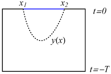
Figure S1: A schematic plot of the domain wall ending at $[x_{1},x_{2}]$ on the $t=0$ boundary. The dashed curve indicates the domain wall. The blue line indicates the boundary with twisted boundary conditions.

As we discussed in the main text, the entanglement entropy can be mapped to the free energy cost of domain walls induced by the twisted boundary condition. A schematic plot of the domain wall induced by the twisted boundary condition within $[x_{1},x_{2}]$ at $t=0$ is shown in Fig. S1. The domain wall is given by the function $y(x)\in[-T,0]$, and its free energy reads

$$S_{A}=-\log\int_{y(x_{1})=y(x_{2})=0}Dye^{-\int dx\left(\sigma\sqrt{1+(\partial_{x}y)^{2}}+V(y)\right)},$$ (S30)

where $\sigma$ is the surface tension and $V(y)$ will be specified below. Let us assume the fluctuation is small so that we can approximate $\sqrt{1+(\partial_{x}y)^{2}}\approx 1+\frac{1}{2}(\partial_{x}y)^{2}$. Then we can calculate the entanglement entropy by mapping it to a transition amplitude of a non-relativistic particle with mass $\frac{1}{2\sigma}$ in a potential

$$\int_{y(x_{1})}^{y(x_{2})}Dye^{-\int dx\left(\frac{\sigma}{2}(\partial_{x}y)^{2}+V(y)\right)}=\langle y(x_{2})|e^{-H(x_{2}-x_{1})}|y(x_{1})\rangle,$$ (S31)

with $H=\frac{1}{2\sigma}p_{y}^{2}+V(y)$, where $y$ and $p_{y}$ are conjugate variables, $[y,p_{y}]=i$.

In the quantum mechanical picture, we use $y$ to denote the depth of the circuit (or the evolution time of the circuit). We will be interested in two cases, $V_{+}(y)$ and $V_{-}(y)$, where the magnetic field exists near the boundary and the potential favors and disfavors the domain wall,

$$V_{+}(y)=\begin{cases}\infty&0<y\\ -hy&-T_{h}<y<0\\ hT_{h}&-T_{h}-T<y<-T_{h}\\ \infty&y<-T_{h}-T\end{cases},\quad V_{-}(y)=\begin{cases}\infty&0<y\\ hy&-T_{h}<y<0\\ -hT_{h}&-T_{h}-T<y<-T_{h}\\ \infty&y<-T_{h}-T\end{cases}.$$ (S32)

Figure S2: Illustration of two kinds of the eigen-energy in the WKB method in the two potentials $V_{+}(y)$ (a) and $V_{-}(y)$ (b).

The potential $V_{+}(y)$ corresponds to the potential felt by the domain wall shown in Fig. S2(a), while the second potential $V_{-}(y)$ corresponds to the potential felt by the domain wall shown in Fig. S2(b). We use the WKB method to calculate the transition amplitude. The approximate energy is given by the formula

$$\int_{y_{1}}^{y_{2}}dy\sqrt{2\sigma(E_{n}-V(y))}=\left(n-\frac{1}{2}\right)\pi,$$ (S33)

where $y_{1}<y_{2}$ are two turning points. There are two types of eigenstates, with energy greater or less than the linear potential, as shown in Fig. S2. For the potential $V_{+}(y)$ the first type of eigenstate is trapped in the linear potential and presents the domain wall located in the region with magnetic field. It has turning point $[-E^{(1)}_{n}/h,0]$, and its eigen-energy is given by

$$\int_{-E^{(1)}_{n}/h}^{0}dy\sqrt{2\sigma(E^{(1)}_{n}+hy)}=\left(n-\frac{1}{2}\right)\pi,$$ (S34)

$$E^{(1)}_{n}=\left(\frac{h^{2}}{2\sigma}\right)^{1/3}\left(\frac{3\pi}{4}(2n-1)\right)^{2/3},\quad 1\leq n\leq n_{*},\quad E_{n_{*}}^{(1)}=hT_{h}.$$ (S35)

It is apparent that $n_{*}$ is independent of $L$. The second type of eigenstate extends to the flat potential and presents the domain wall that form in the region without magnetic field. It has turning point $[-T-T_{h},0]$, and its eigenenergy is determined by

$$\int_{-T_{h}}^{0}dy\sqrt{2\sigma(E^{(2)}_{n}+hy)}+\int_{-T_{h}}^{-T_{h}-T}dy\sqrt{2\sigma(E^{(2)}_{n}-hT_{h})}$$ (S36)

$$=\frac{2}{3}\left(\frac{2\sigma}{h^{2}}\right)^{1/2}\left((E^{(2)}_{n})^{3/2}-(E^{(2)}_{n}-hT_{h})^{3/2}\right)+\sqrt{2\sigma(E^{(2)}_{n}-hT_{h})}T=n\pi,$$ (S37)

$$E^{(2)}_{n}=hT_{h}+\frac{1}{2\sigma}\left(\frac{n\pi}{T}\right)^{2},\quad E^{(2)}_{n}\gg hT_{h},$$ (S38)

where in the second line we have replaced $n+\frac{1}{2}$ by $n$ because we know that the turning point is actually a node, and in the last line we make the approximation $E^{(2)}_{n}\gg hT_{h}$. The transition amplitude reads

$$\langle y(x_{2})|e^{-H_{+}(x_{2}-x_{1})}|y(x_{1})\rangle=\sum_{n=1}^{\infty}e^{-E_{n}(x_{2}-x_{1})}\psi^{\ast}_{n}(-\epsilon)\psi_{n}(-\epsilon)$$ (S39)

$$= \sum_{n=1}^{n_{\ast}}e^{-E^{(1)}_{n}(x_{2}-x_{1})}\psi^{(1)\ast}_{n}(-\epsilon)\psi^{(1)}_{n}(-\epsilon)+\sum_{n=1}^{\infty}e^{-E^{(2)}_{n}(x_{2}-x_{1})}\psi^{(2)\ast}_{n}(-\epsilon)\psi^{(2)}_{n}(-\epsilon),$$

$$\approx e^{-\left(\frac{3\pi}{4}\right)^{2/3}\left(\frac{h^{2}}{2\sigma}\right)^{1/3}x_{12}}\sum_{n=1}^{n_{\ast}}\psi^{(1)\ast}_{n}(-\epsilon)\psi^{(1)}_{n}(-\epsilon)+e^{-hT_{h}x_{12}}\sqrt{\frac{2}{\pi}}\epsilon^{2}(2\sigma)^{3/2}x_{12}^{-3/2},$$ (S40)

where in the last step, we approximate the wave function $\psi^{(2)}_{n}(y)$ by the eigenstate of a infinite potential box $\psi^{(2)}_{n}(y)=\sqrt{\frac{2}{T}}\sin\frac{n\pi y}{T}$, and extends the summation by an integral. Because we use the large-$N$ approximation to get the domain wall free energy, the $N$ should be restored by taking $\sigma\rightarrow N\sigma$ and $h\rightarrow Nh$. Thus the first term in (S40) dominates in the large-$N$ limit, and the transition amplitude reads,

$$\langle y(x_{2})|e^{-H_{+}(x_{2}-x_{1})}|y(x_{1})\rangle \approx e^{-N^{1/3}\left(\frac{3\pi}{4}\right)^{2/3}\left(\frac{h^{2}}{2\sigma}\right)^{1/3}x_{12}}\sum_{n=1}^{n_{\ast}}\psi^{(1)\ast}_{n}(-\epsilon)\psi^{(1)}_{n}(-\epsilon)\sim e^{-N^{1/3}\left(\frac{3\pi}{4}\right)^{2/3}\left(\frac{h^{2}}{2\sigma}\right)^{1/3}x_{12}}.$$ (S41)

The domain wall of the first type has the free energy

$$F_{a}(x_{12})=N\sigma x_{12}+N^{1/3}\left(\frac{3\pi}{4}\right)^{2/3}\left(\frac{h^{2}}{2\sigma}\right)^{1/3}x_{12}\approx N\sigma x_{12}.$$ (S42)

Now a similar analysis for the potential $V_{-}(y)$ can be lay out. For the potential $V_{-}(y)$ the first type of eigenstate is trapped in the linear potential and presents the domain wall located in the region with magnetic field. It has turning point $[-T-T_{h},E^{(1)}/h]$, and its eigen-energy is given by

$$\int_{-T-T_{h}}^{-T_{h}}dy\sqrt{2\sigma(E^{(1)}_{n}+hT_{h})}+\int_{-T_{h}}^{E^{(1)}_{n}/h}dy\sqrt{2\sigma(E^{(1)}_{n}-hy)}$$ (S44)

$$= T\sqrt{2\sigma(E^{(1)}_{n}+hT_{h})}+\frac{2}{3}\left(\frac{2\sigma}{h^{2}}\right)^{1/2}\left(hT_{h}+E_{n}^{(1)}\right)^{3/2}=\left(n-\frac{1}{2}\right)\pi,$$

$$E^{(1)}_{n}=-hT_{h}+f\left((n-\frac{1}{2})\pi\right),\quad 1\leq n\leq n_{*},\quad E_{n_{*}}^{(1)}=0.$$

where $f$ is the solution to $T\sqrt{2\sigma f}+\frac{2}{3}\left(\frac{2\sigma}{h^{2}}\right)^{1/2}f^{3/2}=\left(n-\frac{1}{2}\right)\pi$. The second type of eigenstate extends to the flat potential and presents the domain wall that form in the region without magnetic field. It has turning point $[-T-T_{h},0]$, and its eigenenergy is determined by

$$\int_{-T_{h}}^{0}dy\sqrt{2\sigma(E^{(2)}_{n}-hy)}+\int_{-T_{h}}^{-T_{h}-T}dy\sqrt{2\sigma(E^{(2)}_{n}+hT_{h})}$$

$$=\frac{2}{3}\left(\frac{2\sigma}{h^{2}}\right)^{1/2}\left((E^{(2)}_{n}+hT_{h})^{3/2}-(E^{(2)}_{n})^{3/2}\right)+\sqrt{2\sigma(E^{(2)}_{n}+hT_{h})}T=n\pi,$$ (S45)

$$E^{(2)}_{n}=-hT_{h}+\frac{1}{2\sigma}\left(\frac{n\pi}{T}\right)^{2},\quad E^{(2)}_{n}\gg hT_{h},$$ (S46)

where in the second line we have replaced $n-\frac{1}{2}$ by $n$ for the same reason, and in the last line we make the approximation $E^{(2)}_{n}\gg hT_{h}$. The transition amplitude reads

$$\langle y(x_{2})|e^{-H_{-}(x_{2}-x_{1})}|y(x_{1})\rangle=\sum_{n=1}^{\infty}e^{-E_{n}(x_{2}-x_{1})}\psi^{\ast}_{n}(-\epsilon)\psi_{n}(-\epsilon)$$ (S47)

$$= \sum_{n=1}^{n_{\ast}}e^{-E^{(1)}_{n}(x_{2}-x_{1})}\psi^{(1)\ast}_{n}(-\epsilon)\psi^{(1)}_{n}(-\epsilon)+\sum_{n=1}^{\infty}e^{-E^{(2)}_{n}(x_{2}-x_{1})}\psi^{(2)\ast}_{n}(-\epsilon)\psi^{(2)}_{n}(-\epsilon),$$ (S48)

$$\approx e^{hT_{h}x_{12}}\left(e^{-f((n-\frac{1}{2})\pi)x_{12}}\sum_{n=1}^{n_{\ast}}\psi^{(1)\ast}_{n}(-\epsilon)\psi^{(1)}_{n}(-\epsilon)+\sqrt{\frac{2}{\pi}}\epsilon^{2}(2\sigma)^{3/2}x_{12}^{-3/2}\right),$$ (S49)

where in the last step, we approximate the wave function $\psi^{(2)}_{n}(y)$ by the eigenstate of a infinite potential box $\psi^{(2)}_{n}(y)=\sqrt{\frac{2}{T}}\sin\frac{n\pi y}{T}$, and extends the summation by an integral. Then after restoring the factor of $N$, we have the transition amplitude with potential $V_{-}(y)$,

$$\langle y(x_{2})|e^{-H_{-}(x_{2}-x_{1})}|y(x_{1})\rangle \sim e^{NhT_{h}x_{12}}.$$ (S50)

The domain wall of the second type has the free energy

$$F_{b}(x_{12})=N\sigma x_{12}-NhT_{h}x_{12}.$$ (S51)

(S42) and (S51) give (12) in the main text.

VI Domain wall picture in the Hayden-Preskill protocol

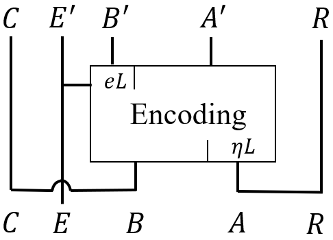
Figure S3: The schematic plot of the encoding process. The information is encoded in $A$. And we collect all the information in $B$. To model the encoded information, we introduce a reference $R$ such that $A$ and $R$ are maximally entangled. We also introduce part $C$ that is maximally entangled with $B$ to model the collection of information in $B$. $B^{\prime}$ denotes the erasure error and $E$ is introduced to model the record loss error.

In the main text we discuss the encoding process where no information about the $B$ part of the circuit is known apriori. Here we generalize the discussion to the case where we have the information about the state in $B$ before we encode the information. In the Hayden-Preskill thought experiment, $B$ is the early radiation of the black hole collected by Bob Hayden and Preskill (2007). The encoding process is schematically shown in Fig. S3. Comparing to Fig.4(a) in the main text, the difference is we have collected the information of part $B$, which is modeled by a maximally entangled part $C$. We are still interested in the mutual information between $E^{\prime}B^{\prime}$ and $R$, i.e.,

$$I(E^{\prime}B^{\prime};R)=S_{R}+S_{E^{\prime}B^{\prime}}-S_{E^{\prime}B^{\prime}R}.$$ (S52)

First consider the case with zero measurement rate (thus no record loss error). In this case the decoupling theorem states that the deviation between the density matrix $\rho_{B^{\prime}R}$ and the tensor product density matrix $\rho_{B^{\prime}}\otimes\rho_{R}$ is bounded by $2^{-N(1-e-\eta)L}$ Abeyesinghe et al. (2009). Thus the error threshold is $1-e_{c}-\eta=0$.

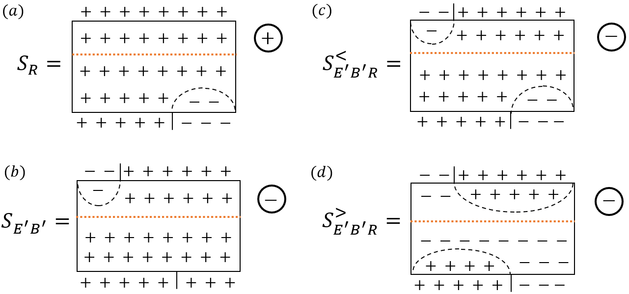
Figure S4: The domain wall configurations corresponding to various quasi entropy, (a) $S_{R}^{(2)}$, (b) $S_{E^{\prime}B^{\prime}}^{(2)}$, and (c,d) $S_{E^{\prime}B^{\prime}R}^{(2)}$ before and after the pinning transition. The $+$ and $-$ indicates $(\phi_{1}\!>\!0,\phi_{2}\!=\!0)$ and $(\phi_{1}\!=\!0,\phi_{2}\!>\!0)$, respectively. The orange dashed line is the boundary of the region with magnetic field, i.e., $T\!<\!t\!<\!T+T_{h}$. The $\pm$ sign in the circle indicates the direction of the magnetic field. Note that there is also a pinning transition in $S_{E^{\prime}B^{\prime}}^{(2)}$, but we only show the configuration before the transition for simplicity.

Now we discuss the domain wall picture of the error threshold from the quasi-2 entropy. As is done in the main text, we can introduce an inaccessible environment to model the record loss error. For each measurement of the $i$-th Majorana in site $x$, if the outcome is not recorded, we can introduce an environment qutrit at $|0_{E}\rangle\langle 0_{E}|$, and the record loss is $\rho\otimes|0_{E}\rangle\langle 0_{E}|\rightarrow U_{E}(\rho\otimes|0_{E}\rangle\langle 0_{E}|)U_{E}^{\dagger}=\sum_{i}M_{i}\rho M_{j}^{\dagger}\otimes|i_{E}\rangle\langle j_{E}|$, where $U_{E}=\sum_{i=1}^{2}M_{i}\otimes\sum_{j=0}^{2}|i_{E}\rangle\langle j_{E}|$. Tracing out the environment will generate an emergent magnetic field. More explicitly, the following trace,

$$\text{Tr}_{E}[(U_{E}|0_{E}\rangle\langle 0_{E}|U_{E}^{\dagger})^{\otimes 2}]=\sum_{i,j}M_{i}\otimes M_{i}^{\dagger}\otimes M_{j}\otimes M_{j}^{\dagger},$$ (S53)

$$\text{Tr}_{E}[(U_{E}|0_{E}\rangle\langle 0_{E}|U_{E}^{\dagger})^{\otimes 2}\mathcal{S}]=\sum_{i,j}M_{i}\otimes M_{j}^{\dagger}\otimes M_{j}\otimes M_{i}^{\dagger},$$ (S54)

where $\mathcal{S}$ is the swap operator, leads to magnetic field pointing along the direction of $\phi_{1}$ (the “$+$” direction) and $\phi_{2}$ (the “$-$” direction), respectively. In $S_{R}^{(2)}$, the environment qutrit is traced out without a swap operator, so the magnetic field is along “$+$” direction. On the other hand, in $S_{E^{\prime}B^{\prime}}^{(2)}$ and $S_{E^{\prime}B^{\prime}R}^{(2)}$, the environment qutrit is traced out with a swap operator, so the magnetic is along “$-$” direction. This is explicitly shown in Fig. S4. The difference between the domain wall picture in the main text and here is the boundary condition of part $B$ in the bottom boundary. Because we have collected the information of $B$ represented by $C$, tracing out $C$ leads to a boundary condition along “$+$” direction in $B$. Including such a modification, $S_{E^{\prime}B^{\prime}R}^{(2)}$ reads

$$S^{(2)}_{E^{\prime}B^{\prime}R}=-\log(e^{-\sigma(e+\eta)L+hT_{h}(1-e)L}+e^{-\sigma(1-e)L}e^{-\sigma(1-\eta)L}).$$ (S55)

The above equation determines the erasure error threshold $e_{c}$ in the presence of the record loss,

$$hT_{h}(1-e_{c})=2\sigma(1-e_{c}-\eta).$$ (S56)

If the measurement rate is zero, and so is the record loss error, i.e., $h=0$, we have reproduced the result of decoupling theorem. Equivalently, if the erasing part is fixed, it is precisely the pinning transition at $h^{*}=\frac{2\sigma}{T_{h}}\frac{1-e-\eta}{1-e}$.

It is worth noting that there is also a similar pinning transition in $S_{E^{\prime}B^{\prime}}^{(2)}$. So including pinning transitions in both $S_{E^{\prime}B^{\prime}R}^{(2)}$ and $S_{E^{\prime}B^{\prime}}^{(2)}$, the mutual information reads

$$I^{(2)}(R;E^{\prime}B^{\prime})=\begin{cases}0&h<h^{*}\\ N[2\sigma(\eta+e-1)+hT_{h}(1-e)]L&h^{*}<h<h^{**}\\ 2N\sigma\eta L&h^{**}<h\end{cases},$$ (S57)

where $h^{**}=\frac{2\sigma}{T_{h}}$ is from the pinning transition of $S_{E^{\prime}B^{\prime}}^{(2)}$. Thus from the domain wall picture of quasi-2 entropy, we have obtained the prediction of error threshold in the Hayden-Proskill protocol in the presence of record-loss error.

References

Li et al. (2018)Y. Li, X. Chen, and M. P. Fisher, Physical Review
B 98, 205136 (2018).
Li et al. (2019)Y. Li, X. Chen, and M. P. Fisher, Physical Review
B 100, 134306 (2019).
Skinner et al. (2019)B. Skinner, J. Ruhman, and A. Nahum, Physical Review
X 9, 031009 (2019).
Choi et al. (2020)S. Choi, Y. Bao, X.-L. Qi, and E. Altman, Physical Review Letters 125, 030505 (2020).
Gullans and Huse (2020a)M. J. Gullans and D. A. Huse, Physical
Review X 10, 041020
(2020a).
Chan et al. (2019)A. Chan, R. M. Nandkishore, M. Pretko, and G. Smith, Physical Review B 99, 224307 (2019).
Zabalo et al. (2020)A. Zabalo, M. J. Gullans,
J. H. Wilson, S. Gopalakrishnan, D. A. Huse, and J. Pixley, Physical Review B 101, 060301 (2020).
Gullans and Huse (2020b)M. J. Gullans and D. A. Huse, Physical
review letters 125, 070606 (2020b).
Li et al. (2020)Y. Li, X. Chen, A. W. Ludwig, and M. Fisher, arXiv preprint arXiv:2003.12721 (2020).
Fan et al. (2020)R. Fan, S. Vijay, A. Vishwanath, and Y.-Z. You, arXiv preprint arXiv:2002.12385 (2020).
Iaconis et al. (2020)J. Iaconis, A. Lucas, and X. Chen, Physical Review B 102, 224311 (2020).
Sang and Hsieh (2020)S. Sang and T. H. Hsieh, arXiv
preprint arXiv:2004.09509 (2020).
Lavasani et al. (2021)A. Lavasani, Y. Alavirad, and M. Barkeshli, Nature Physics , 1 (2021).
Ippoliti et al. (2021)M. Ippoliti, M. J. Gullans, S. Gopalakrishnan, D. A. Huse, and V. Khemani, Physical Review X 11, 011030 (2021).
Chen et al. (2020a)X. Chen, Y. Li, M. P. Fisher, and A. Lucas, Physical Review Research 2, 033017 (2020a).
Alberton et al. (2020)O. Alberton, M. Buchhold, and S. Diehl, arXiv preprint
arXiv:2005.09722 (2020).
Jian et al. (2020)C.-M. Jian, B. Bauer,
A. Keselman, and A. W. Ludwig, arXiv preprint
arXiv:2012.04666 (2020).
Tang et al. (2021)Q. Tang, X. Chen, and W. Zhu, arXiv preprint arXiv:2101.04320 (2021).
Buchhold et al. (2021)M. Buchhold, Y. Minoguchi,
A. Altland, and S. Diehl, arXiv preprint arXiv:2102.08381 (2021).
Bao et al. (2021)Y. Bao, S. Choi, and E. Altman, arXiv preprint arXiv:2102.09164 (2021).
Zhang et al. (2021a)P. Zhang, S.-K. Jian,
C. Liu, and X. Chen, arXiv preprint arXiv:2104.04088
(2021a).
Jian et al. (2021)S.-K. Jian, C. Liu, X. Chen, B. Swingle, and P. Zhang, arXiv preprint arXiv:2104.08270 (2021).
Nielsen and Chuang (2001)M. A. Nielsen and I. L. Chuang, Phys.
Today 54, 60 (2001).
Dennis et al. (2002)E. Dennis, A. Kitaev,
A. Landahl, and J. Preskill, Journal of Mathematical Physics 43, 4452 (2002).
Kitaev (2015)A. Kitaev, talk
given at the KITP Program: entanglement in strongly-correlated quantum
matter (2015).
Sachdev and Ye (1993)S. Sachdev and J. Ye, Physical review
letters 70, 3339
(1993).
Maldacena and Stanford (2016)J. Maldacena and D. Stanford, Physical Review D 94, 106002 (2016).
Liu et al. (2018)C. Liu, X. Chen, and L. Balents, Physical Review B 97, 245126 (2018).
Gu et al. (2017)Y. Gu, A. Lucas, and X.-L. Qi, Journal of High Energy Physics 2017, 1 (2017).
Huang et al. (2019)Y. Huang, Y. Gu, et al., Physical Review D 100, 041901 (2019).
Zhang et al. (2020)P. Zhang, C. Liu, and X. Chen, arXiv preprint arXiv:2003.09766 (2020).
Haldar et al. (2020)A. Haldar, S. Bera, and S. Banerjee, Physical Review Research 2, 033505 (2020).
Zhang (2020)P. Zhang, Journal
of High Energy Physics 2020, 1 (2020).
Chen et al. (2020b)Y. Chen, X.-L. Qi, and P. Zhang, Journal of High Energy Physics 2020, 1 (2020b).
García-García et al. (2021)A. M. García-García, Y. Jia, D. Rosa, and J. J. Verbaarschot, arXiv preprint arXiv:2102.06630 (2021).
Zhang et al. (2021b)P. Zhang, C. Liu, S.-K. Jian, and X. Chen, arXiv preprint arXiv:2105.08895
(2021b).
(37)Technically, the calculable quantity is not
entanglement entropy but the quasi entropy defined in (5). We
expect that the entanglement entropy also has a transition since the quasi
entropy is believed to be a useful proxy of entanglement
entropy.
Li and Fisher (2020)Y. Li and M. Fisher, arXiv preprint
arXiv:2007.03822 (2020).
Gullans et al. (2020)M. J. Gullans, S. Krastanov,
D. A. Huse, L. Jiang, and S. T. Flammia, arXiv preprint arXiv:2010.09775 (2020).
Li et al. (2021)Y. Li, S. Vijay, and M. P. Fisher, arXiv preprint
arXiv:2105.13352 (2021).
Saad et al. (2018)P. Saad, S. H. Shenker, and D. Stanford, arXiv preprint
arXiv:1806.06840 (2018).
Sünderhauf et al. (2019)C. Sünderhauf, L. Piroli, X.-L. Qi,
N. Schuch, and J. I. Cirac, Journal of High Energy Physics 2019, 1 (2019).
Liu et al. (2020)C. Liu, P. Zhang, and X. Chen, arXiv preprint arXiv:2008.11955 (2020).
Jian and Swingle (2020)S.-K. Jian and B. Swingle, arXiv preprint
arXiv:2011.08158 (2020).
Napp et al. (2019)J. Napp, R. L. La Placa,
A. M. Dalzell, F. G. Brandao, and A. W. Harrow, arXiv preprint arXiv:2001.00021 (2019).
(46)See Supplemental Material for: 1. The
large- action and the saddle-point equation for the monitored system. 2.
The effective action of the monitored system in the presence of record-loss
error. 3. Frame potential of the Brownian SYK model. 4. The free energy of
domain walls. 5. Domain wall picture in the Hayden-Preskill
protocol.
(47)In this case we have , , , sup , so we omit the subscript of the left and right
chains.
Penington et al. (2019)G. Penington, S. H. Shenker, D. Stanford, and Z. Yang, arXiv preprint
arXiv:1911.11977 (2019).
(49)Note that the first-order pinning transition
discussed in our paper is different from the second-order pinning transition
between bounded and unbounded domain walls by weakened bonds near the
boundary Abraham (1980).
Schumacher and Nielsen (1996)B. Schumacher and M. A. Nielsen, Physical Review A 54, 2629 (1996).
Onorati et al. (2017)E. Onorati, O. Buerschaper, M. Kliesch, W. Brown,
A. Werner, and J. Eisert, Communications in Mathematical
Physics 355, 905
(2017).
Brandão et al. (2019)F. G. Brandão, W. Chemissany, N. Hunter-Jones, R. Kueng, and J. Preskill, arXiv preprint arXiv:1912.04297 (2019).
(53)We also calculate the frame potential of the
Brownian SYK chain (Quantum error as an emergent magnetic field) without monitoring sup ,
which shows that the Brownian SYK chain can achieve the 2
design.
Abeyesinghe et al. (2009)A. Abeyesinghe, I. Devetak, P. Hayden, and A. Winter, Proceedings of the
Royal Society A: Mathematical, Physical and Engineering Sciences 465, 2537 (2009).
Hayden and Preskill (2007)P. Hayden and J. Preskill, Journal of high energy physics 2007, 120 (2007).
Yoshida and Kitaev (2017)B. Yoshida and A. Kitaev, arXiv
preprint arXiv:1710.03363 (2017).
Abraham (1980)D. Abraham, Physical Review Letters 44, 1165 (1980).
Roberts and Yoshida (2017)D. A. Roberts and B. Yoshida, Journal of High Energy Physics 2017, 121 (2017).