Multi-Modal Prototype Learning for Interpretable Multivariable Time Series Classification

Abstract

Multivariable time series classification problems are increasing in prevalence and complexity in a variety of domains, such as biology and finance. While deep learning methods are an effective tool for these problems, they often lack interpretability. In this work, we propose a novel modular prototype learning framework for multivariable time series classification. In the first stage of our framework, encoders extract features from each variable independently. Prototype layers identify single-variable prototypes in the resulting feature spaces. The next stage of our framework represents the multivariable time series sample points in terms of their similarity to these single-variable prototypes. This results in an inherently interpretable representation of multivariable patterns, on which prototype learning is applied to extract representative examples i.e. multivariable prototypes. Our framework is thus able to explicitly identify both informative patterns in the individual variables, as well as the relationships between the variables. We validate our framework on a simulated dataset with embedded patterns, as well as a real human activity recognition problem. Our framework attains comparable or superior classification performance to existing time series classification methods on these tasks. On the simulated dataset, we find that our model returns interpretations consistent with the embedded patterns. Moreover, the interpretations learned on the activity recognition dataset align with domain knowledge.

1 Introduction

Multivariable time series classification aims to leverage the measurement of multiple variables over a period of time to assign data points to classes. As such, these problems arise naturally across various domains, including biology [1], finance [2], and activity recognition [1]. Along with their increased prevalence, multivariable time series classification datasets have increased in size and complexity, making their analysis challenging [3]. Internet-of-Things technologies, for example, allow for the connection of multiple sensing devices [4]. These device networks generate datasets and classification tasks involving a large number of sensors, many with markedly different characteristics [5]. Similarly, developments in biosensing technologies have given rise to the multi-modal biosensing problem, where time series readings from a diverse set of biosensors are used to characterize the mental and physical state of a subject. Biosensing has been applied in sleep staging [6], emotion recognition [7, 8], stress detection [9], attention studies [10, 11], brain-computer interfaces [12, 13], and wellness monitoring [14, 15]. These problems predominantly arise in research settings, with the goal of deriving scientific knowledge from the data. As such, model interpretability is of central importance.

Due to its wide applicability, multivariable time series classification is an area of active research and a multiplicity of approaches exist. These approaches can be divided into deep-learning based methods and feature-based methods. Many feature-based time series classification methods utilize hand-crafted feature extraction techniques. For example, in [1], discrete features learned from the multivariable time series are used to construct a bag-of-patterns model for classification. Deep learning based methods do not rely on hand-crafted features, instead learning an end-to-end model. In [16] for example, a combination of recurrent and convolutional neural networks are proposed for the problem of EEG classification in a brain-computer interface setting. Deep learning techniques are an increasingly powerful tool for dealing with the rising complexity of multivariable time series classification problems. Although deep learning methods are able to learn complex relationships, it is difficult to reveal these relationships in a human-understandable way. This is primarily due to the high number of parameters of deep learning models, and the large space of functions that they could represent [17, 18].

There are two major challenges in interpretable multivariable time series classification: heterogeneity in the variables and cross-variable patterns. Many multivariable time series classification datasets are comprised of variables with vastly different noise levels, time scales, and feature domains. For example, in the multi-modal bio-sensing problem, signals representing vastly different biological processes are combined into a single dataset. Moreover, in multivariable settings, it is generally necessary to combine information from multiple variables to arrive at a final classification. As a result, a successful interpretation framework must reveal both the relevant patterns at the single-variable level and the patterns present across variables.

This paper introduces a modular, multi-layer prototype learning framework for interpretable classification on multivariable time series data. Our framework provides model-based interpretability, as it is designed to produce classifications transparently [19]. In the framework, single-variable encoders are trained by contrastive learning to extract meaningful features from each variable. Next, single-variable prototype layers represent sample points in terms of their similarity to a set of learned single-variable prototypes. The single-variable prototype similarities are concatenated over all variables, yielding an inherently interpretable representation of the interactions between variable level patterns and a second prototype layer identifies meaningful rules in the form of multivariable prototypes. Taken together, the single-variable and multivariable prototypes show how patterns at the variable level combine together to characterize classes.

The contributions of this work are three fold. First, we present a novel interpretable method for multivariable time series classification which explicitly models both individual variable patterns as well as cross variable patterns. Second, we provide a step-wise training procedure for effectively training the multi-level prototype model. Finally, we design a synthetic dataset with heterogeneous variables and cross variable patterns to verify the validity of the interpretations, as well as demonstrating the applicability of our method on a real-world human activity recognition problem.

2 Related Literature

Multivariable time series classification has been studied extensively and various classification techniques have been proposed in different domains. In this section, we introduce some of these related works with a specific emphasis on interpretability. We divide these prior works into feature based approaches and neural network based approaches.

Feature Based Approaches

Feature based methods generally rely on manual feature extraction methods and discretization to extract features from time series streams. An important class of these methods are Bag-of-Pattern (BOP) methods. BOP methods generate symbolic features from time series sub sequences and represent signals using a bag-of-words like symbol histogram. In [1], Symbolic Fourier Approximation (SFA) is applied to each dimension of a multivariable time series classification problem. The univariate symbolic representations are then combined to generate a multivariable Bag-of-Patterns representation. In [20], a random-forest learner is used to generate symbols for a multivariable bag-of-patterns method. Another important class of feature based approaches are Shapelet methods. These approaches involve extracting time series subsequences that are highly relevant for classification, called shapelets. [21] presents a more efficient method for extracting shapelets from large multivariable datasets by pruning similar shapelet candidates. In [22], multivariate shapelets are used for early classification of signals. Notably, shapelet based methods often have favourable interpretability properties, as the shapelets themselves are directly interpretable as characteristic patterns. However, both shapelet and discretization approaches can be slow and generate potentially very large feature spaces.

Neural Network Approaches

Neural network based approaches harness the ability of neural networks to learn complex functions as a feature extraction technique. Some of these methods, however, use neural networks in conjunction with discretization and feature extraction approaches. In [23], SFA features are fed through a neural network to project them into an encoded space. Prototype learning on the encoded space is used for the final classification. In [24], a recurrent neural network encoder produces feature vectors for a prototype learning classifier. In this method, the learned prototypes are used for interpretability purposes. [25] uses random dimension permutation with an attentional prototype network for multivariable time series classification but does not address interpretability. Finally, [26] learns interpretable multivariate shapelets in an embedded space over all dimensions of the multivariable classification problem. Our method builds upon these methods through two levels of prototype learning. This allows for more complex cross variable interactions to be represented, as well as explicitly modelling the informative variation in each variable.

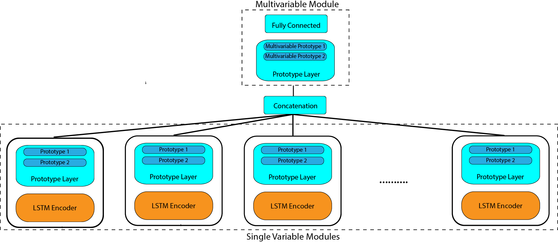
Figure 1: Schematic of the proposed framework. The time series corresponding to each variable are separated and input to their respective single-variable encoding layers. These encoded representations are compared to a set of learned prototypes in the single-variable prototype layer, generating a prototype similarity vector for each variable. A multivariable representation of the time series is created by concatenating the prototype similarity vectors from all the variables. The multivariable representation is then compared to a set of multivariable prototypes, yielding a multivariable prototype similarity vector. This multivariable prototype similarity vector is input to a fully connected softmax network to generate the final classification.

3 Model

We propose a two-level encoder-prototype learning method for multivariable time series classification.

Problem Formulation

Consider a multivariable time series classification task containing $d$ dimensions and $n$ time samples per dimension and a dataset $D=\{(\mathbf{X^{(i)}},y_{i})\}$, where $y_{i}\in\mathbb{Z}$ denotes the label for training example $i$ and $\mathbf{X^{(i)}}\in\mathbb{R}^{n\times d}$ is a matrix for time series sample point $i$. Each row of $\mathbf{X^{(i)}}$ is a time point and each column represents a variable. In particular, we can write $\mathbf{X^{(i)}}=\begin{bmatrix}\mathbf{x^{(i)}_{1}}&...&\mathbf{x^{(i)}_{d}}\end{bmatrix}$, where $\mathbf{x^{(i)}_{k}}\in\mathbb{R}^{n}$ -represents the time series corresponding to the $k$-th variable. The multi-variable time series classification problem aims to learn a function $f:\mathbb{R}^{n\times d}\to\mathbb{Z}$, which maps instances of the multi-variable time series to their correct class.

Single-Variable Encoder

First, our method performs feature extraction independently for each variable. Feature extraction is accomplished by a set of single-variable encoder networks each of which maps a particular variable’s time series signal to an encoded vector representation. In this work, we utilize a LSTM encoder network for time series feature extraction, however the choice of encoding network is entirely flexible and can be tuned using domain knowledge. Concretely, our model learns a set of encoder functions $\{E_{1},...,E_{d}\}$, $E_{k}:\mathbb{R}^{n}\to\mathbb{R}^{f_{k}}$ mapping raw time series data for variable $k$ into a feature space of dimension $f_{k}$. We denote the encoding for variable $k$ for some sample point $\mathbf{X}=\begin{bmatrix}\mathbf{x}_{1},...,\mathbf{x}_{d}\end{bmatrix}$ as $\mathbf{e_{k}}\in\mathbb{R}^{f_{k}}$ and have that $\mathbf{e_{k}}=E_{k}(\mathbf{x_{k}})$.

Single-Variable Prototype Matching Layer

Following the single-variable encoding step, our method learns informative patterns in each variable and represents data points in terms of their similarity to these informative patterns. This is achieved by way of a single-variable prototype matching layer. We define a prototype matching layer for the $k$-th variable as a function $P_{k}:\mathbb{R}^{f_{k}}\to\mathbb{R}^{n_{k}}$ parametrized by a set of $n_{k}$ prototype vectors $\{\mathbf{p}^{(k)}_{1},...,\mathbf{p}^{(k)}_{n_{k}}\}$ in the feature space for variable $k$. $P_{k}$ maps vectors from variable $k$’s feature space to a vector of similarity scores with each of the prototype vectors. Explicitly, for the encoded vector $\mathbf{e_{k}}$, we have that $P_{k}(\mathbf{e_{k}})=\begin{bmatrix}\text{sim}(\mathbf{e}_{k},\mathbf{p}^{(k)}_{1}),...,\text{sim}(\mathbf{e}_{k},\mathbf{p}^{(k)}_{n_{k}})\end{bmatrix}$, for a similarity function sim. In this work, we consider $\text{sim}(\mathbf{v_{1}},\mathbf{v_{2}})=\frac{1}{||\mathbf{v_{1}}-\mathbf{v_{2}}||_{2}}$.

Multivariable Prototype Matching Layer

Using the single-variable similarity vectors, our model constructs an inherently interpretable representation of a multivariable time series instance in terms of the learned single-variable prototypes. This is achieved by concatenating together the prototype similarity vectors across all the variables, thus showing the combination of variable level patterns. Formally, a multivariable time series sample point $\mathbf{X}\in\mathbb{R}^{n}$ is represented as a multivariable representation vector $\mathbf{m}=P_{1}(\mathbf{e_{1}})\oplus...\oplus P_{k}(\mathbf{e_{k}})$ where $\oplus$ denotes the concatenation operation, so $\mathbf{m}\in\mathbb{R}^{\sum\limits_{k=1}^{d}n_{k}}$. As a result of this construction, the multivariable representation can be viewed as a series of blocks corresponding to each variable. We introduce an additional prototype learning layer on the multivariable representation space in order to learn prototypical rules detailing the interactions between variable level prototypes. The multivariable prototype learning layer, denoted as $P_{M}:\mathbb{R}^{\sum\limits_{k=1}^{d}n_{k}}\to\mathbb{R}^{n_{M}}$ is parametrized by a set of $n_{M}$ multivariable prototypes, $\{\mathbf{p_{1}^{(M)}},...,\mathbf{p_{n_{M}}^{(M)}}\}$ which are learned during training. $P_{M}$ maps the multivariable vector $\mathbf{m}$ to a vector of its similarities with the multivariable prototype vectors. Thus, we have that $P_{M}(\mathbf{m})=\begin{bmatrix}\text{sim}(\mathbf{p_{1}^{(M)}},\mathbf{m})&...&\text{sim}(\mathbf{p_{1}^{(M)}},\mathbf{m})\end{bmatrix}$. We produce predictions by passing the multivariable prototype similarity vector through a fully connected neural network with softmax activation.

3.1 Objective and Regularization

Our model utilizes Cross Entropy loss as the objective for the classification task. However, additional regularization must be added in order to ensure that the learned prototype vectors at both the single and multivariable levels are meaningful and easy to interpret. We make use the following regularization terms which were introduced in [24]:

Prototype Diversity

We utilize the prototype diversity loss shown in Equation 1 in order to ensure that the prototypes learned by the prototype matching layers represent unique points in the encoded space. This is important for intepretability as duplicate prototypes do nothing to enhance the quality of interpretation, while also damaging the stability of the interpretations. The utilization of the logarithm in this loss function ensures that the penalty does not quickly vanish. This function yields a high penalty to close by prototypes and a low penalty to those that are farther away [24].

$$L_{diversity}=\frac{1}{\log\frac{1}{m}\sum\limits_{j=1}^{m}\min\limits_{i>j}||p_{i}-p_{j}||}$$ (1)

Prototype Similarity

As in related works on time series classification prototype learning, such as [26] and [23], prototype vectors are interpreted in this work by projection onto the training set. In order to ensure that this projection step results in a meaningful representation of the prototype, it is important that each prototype is similar to one of the encoded training examples. We include the regularization term in Equation 2 in order to penalize the distance between each prototype and its closest training example. This encourages every prototype to be close to at least one training example, such that that training example can be considered a meaningful representation of the prototype during projection [24].

$$L_{similarity}=\sum\limits_{j=1}^{m}\min\limits_{i\in[1,n]}||p_{j}-f(x_{i})||$$ (2)

Encoded Space Coverage

The interpretability and classification performance of prototype learning hinges on all data points being well-represented by the learned prototype set. Thus we include the coverage regularization term in Equation 3, in order to ensure that the learned prototypes adequately cover the entirety of the encoded training points. This term, which penalizes the distance between every encoded training example and its closest prototype, penalizes learned prototype sets which neglect certain regions of the encoded space [24].

$$L_{coverage}=\sum\limits_{j=1}^{n}\min\limits_{i\in[1,m]}||p_{i}-f(x_{j})||$$ (3)

3.2 Training Procedure

Encoder Pretraining

In order for meaningful prototypes to be selected for each variable, the encoder should be able to extract information from the samples that is meaningful in the classification task. To this end, we propose a pre-training step for the encoders based on contrastive learning [27]. During the contrastive learning stage, pairs of training examples are input into the encoder and their encodings are computed. These pairs of training examples are used to compute the contrastive loss function shown in Equation 4 and the encoder is trained to minimize this loss function. This contrastive loss function encourages training examples of the same class to be mapped close to each other in the encoded space, and training examples from different classes to be mapped farther away.

$$L_{contrastive}= \frac{1}{2}(1-y)||f(x_{1})-f(x_{2})||_{2}^{2}+ \frac{1}{2}(y)\max{(0,m-||f(x_{1})-f(x_{2})||_{2})}^{2}$$ (4)

Single-Variable Module Training

In the next part of the training process, the single-variable prototype matching layers are trained, resulting in a set of representative prototypes being learned for each variable. Although it seems appropriate to train both the single-variable prototype matching layers and the multivariable prototype matching layer together, this end to end approach yields poor results. Thus, the training of the two units is completed separately. In order to train the single-variable prototype matching layers, we construct a new network where the outputs of all the prototype matching layers are concatenated and fed through a fully connected layer to determine a final classification output. This new network is then trained with the cross entropy loss objective, along with the appropriate regularization terms applied to the single-variable prototype matching layers. This new network allows the single-variable prototype matching layers to be trained taking into account the interactions between variables, while avoiding the challenges posed by end to end training.

Multivariable Module Training

In the final stage of training, the multivariable prototype matching and classification layers are trained on the cross entropy loss, along with interpretability regularizers applied to the multivariable prototype matching layer. As was noted previously, only the parameters of the multivariable prototype matching layer and classification layer are subject to update in this stage, all other parameters are frozen.

4 Evaluation

We evaluate our framework on the following datasets to verify its ability to both classify with high performance and reveal meaningful interpretations. For these experiments, we utilize the PyTorch deep learning library [28]. All experiments were conducted on an Apple 2015 MacBook Pro with an Intel i7 processor.

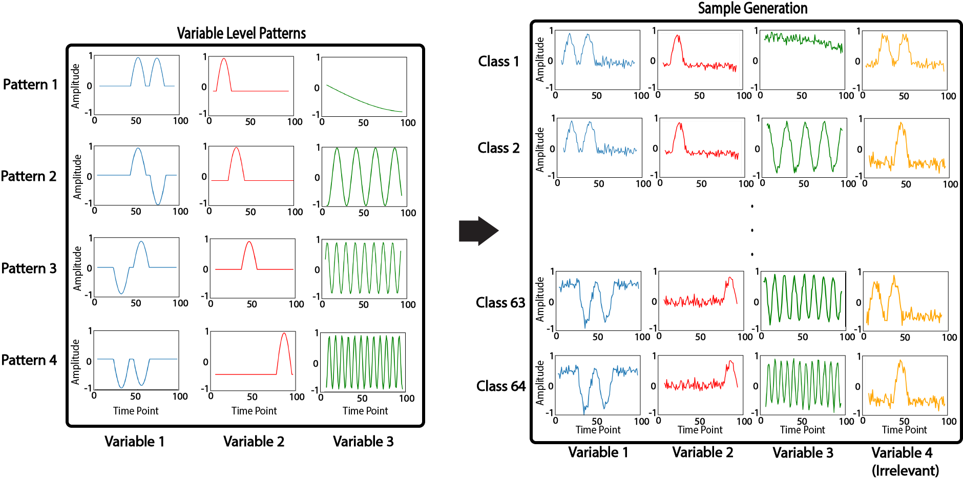
Figure 2: Schematic showing the construction of the simulated dataset. Each of the relevant variables has 4 possible patterns, as displayed in the variable level pattern box (left). Each class is a unique combination of one variable level pattern taken from each variable, as shown in the sample generation box (right). The sample generation box also shows the addition of sample noise to the dataset, as well as the randomly sampled irrelevant variable.

Generation of the Dataset

Our simulated dataset contains four variables. Three of these variables are designed to contain meaningful information for the classification task, whereas one of the variables is designed to be irrelevant noise. In order to test the flexibility of our framework in processing time series signals, each of the three relevant variables contains a different type of time series pattern. The first variable contains patterns that are localized to a subsection of the total time series, but are shift invariant - the location of the pattern sub sequence relative to the entire time series should not affect classification. The second variable contains patterns that are also restricted to a sub sequence of the time series but are shift variant - the location of the pattern sub sequence with respect to the entire time series is meaningful. Finally, the last relevant variable contains a frequency domain pattern. Each of the three meaningful variables has four patterns states that it can exhibit, as shown in the Figure 2. We refer to these states as variable-level patterns.

A particular class in the simulated dataset is determined by the combination of the patterns found in the three variables. We create a class corresponding to each combination of variable-level patterns in the relevant variables, resulting in $4^{3}=64$ classes. As a result of this design, the contributions of all three relevant variables are necessary to correctly classify a point. During sample generation, 100 points are generated per class and appropriate types of noise are added to each variable. In addition, the irrelevant variable is randomly sampled from a set of patterns, independently of the class.

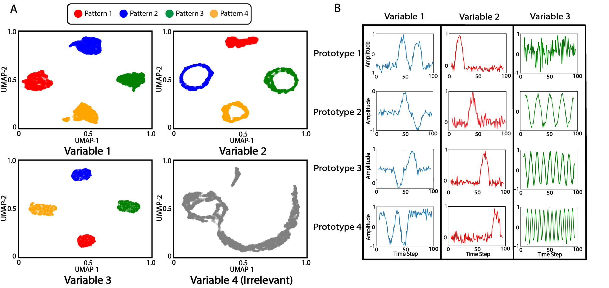
Figure 3: (A) 2-dimensional UMAP visualization of the training set encodings corresponding to each variable. Variables 1,2, and 3 are relevant for classification and thus sample points are colored by the variable-level pattern exhibited in the variable. (B) Representation of the single-variable prototypes by projection onto the dataset. Each prototype is represented by the training point that lies closest to it in the encoded space.

Single-Variable Encoded Spaces and Prototypes

On the simulated dataset, our framework is able to consistently achieve 1.00 hold-out test set classification accuracy, as is expected from the prescribed structure present in the dataset. In order to investigate interpretability, we begin by visualizing the encoded space corresponding to each variable using UMAP [29] in Figure 3.A. The encoded spaces for the three relevant variables each contain 4 clusters and each cluster corresponds to one of the variable-level patterns implanted in the dataset. The irrelevant variable, on the other hand, does not exhibit the same structure because it does not contain any relevant information for classification.

In the simulated dataset, the time series signal in any given variable alone is insufficient to classify the data point. As such, it is notable that the contrastive loss training step, which only takes into account the classes of the data points and treats each variable independently, is able to learn about the underlying patterns present in each variable. This demonstrates the effectiveness of the contrastive loss training even in the case where classes can only be determined by integrating information across the several variables.

For the simulated dataset, the number of single-variable prototypes was set to four by validation. The result of the single-variable prototype learning is shown in the Figure 3.B. As is seen by comparing Figure 3.B and Figure 2, in each relevant variable, there is one prototype corresponding to each of the implanted variable-level patterns.

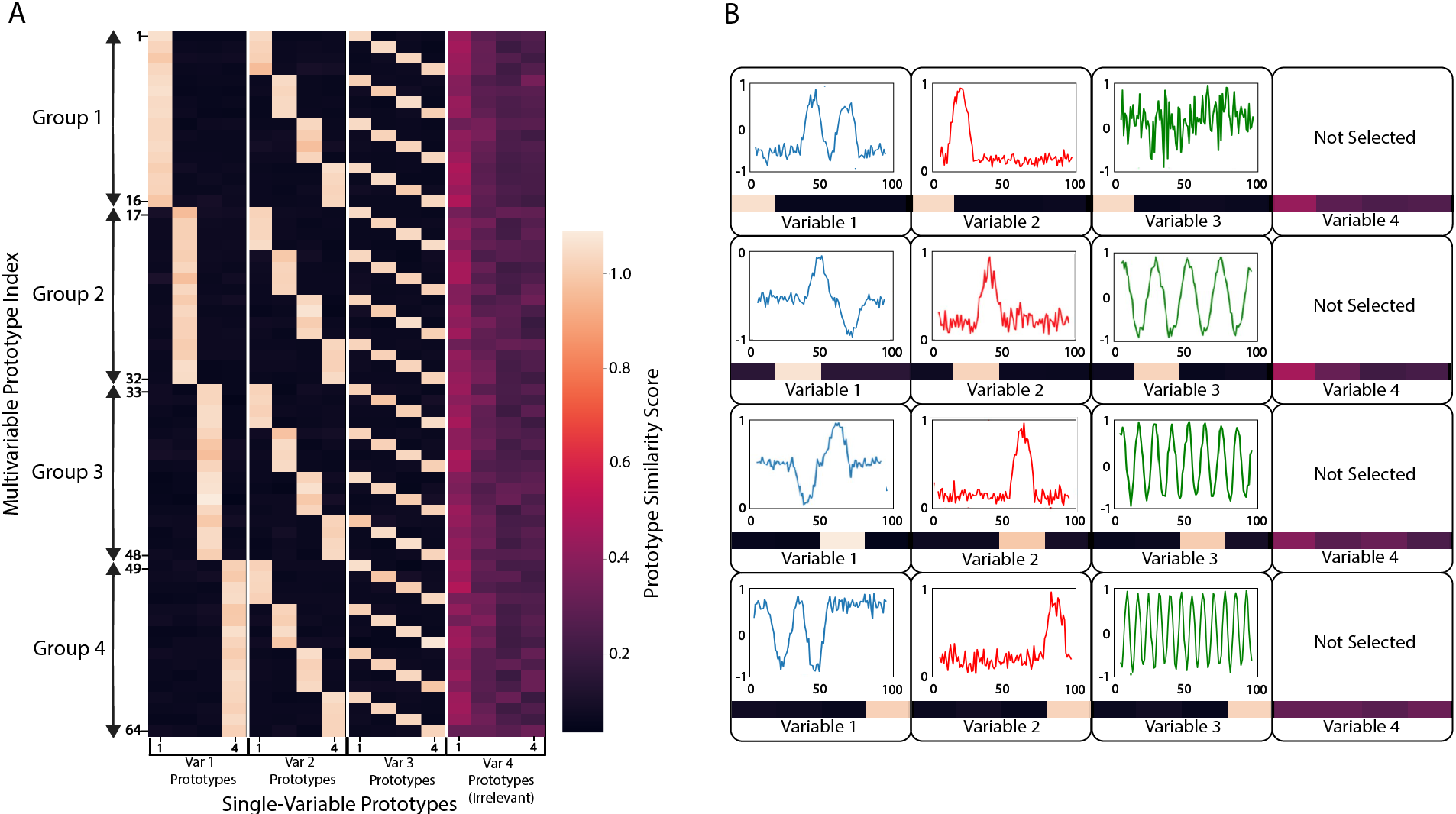
Figure 4: (A) Visualization of all 64 multivariable prototype vectors for the simulated dataset in a heat map. The prototypes are ordered by the class number they represent. (B) Interpretation examples for select multivariable prototypes. The multivariable prototype vectors are separated into the variable blocks. The projection of the single-variable prototype with the highest prototype similarity score is shown for each variable, except variable 4 which has low, uniform values.

Multivariable Prototypes

We set the number of multivariable prototypes to 64, as there are 64 classes. The learned prototypes are presented in the heat map shown in Figure 4.A, where each row of the heat map shows one prototype. Our framework learns one prototype corresponding to each class. In the blocks corresponding to the three relevant variables, the prototype vector for a given class gives a one-hot encoded representation of the single-variable patterns used in constructing that class. On the other hand, the block corresponding to the irrelevant variable shows low, uniform values, indicating that there is no preference for a particular pattern in this variable given the class. Thus, we observe that the implanted patterns in this dataset are explicitly recovered in an easy to understand way by our framework. Figure 4.B shows examples of using the multivariable prototypes in conjunction with the single-variable prototypes for interpretation.

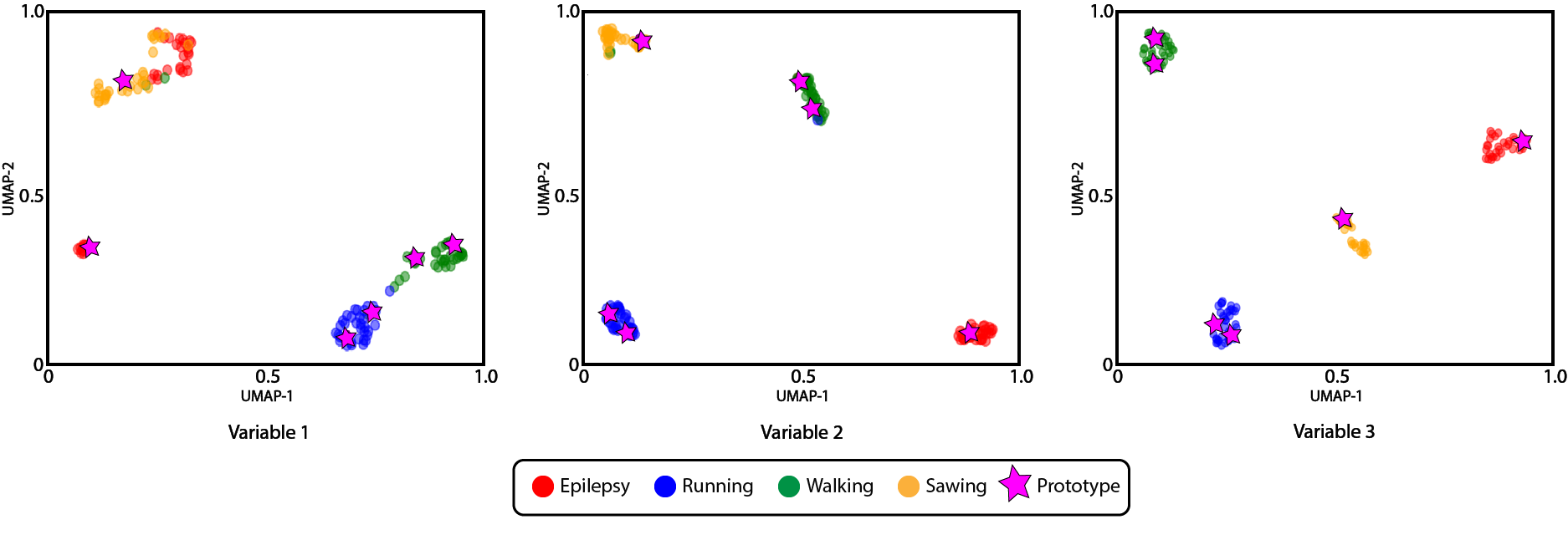
Figure 5: 2-dimensional UMAP visualization of the single-variable encoded spaces and prototypes for the Epilepsy classification task. Training set sample points are colored by the class they belong to and the locations of the learned prototype vectors are depicted by the magenta stars.

4.1 Epilepsy Dataset

In order to validate the method on a real-world classification problem, we selected the Epilepsy dataset in the UEA Time Series repository [30]. The dataset consists of triaxial accelerometer data collected from the dominant wrist of subjects completing four activities: running, walking, sawing, and seizure mimicking [31]. Each activity lasts for 30 seconds and the accelerometer sampling rate is 16 Hz [31]. The classification objective is to predict the activity from the accelerometer readings.

Encoded Space Visualization and Single-Variable Prototypes

Our framework is able to achieve 0.94 accuracy with a standard deviation of 0.04 on the hold-out test set, comparable to existing time series classification methods [30]. To examine the single-variable encoded spaces and prototypes, we use the UMAP technique, as shown in Figure 5. As seen in the figure, each class has a cluster in variables 2 and 3, indicating that the classes are easily distinguishable in these variables. In variable 1, the running and walking class data points lie in their own clusters, while the epilepsy and sawing classes overlap. Moreover, the epilepsy class is split into two clusters which indicates that there are multiple patterns in the first variable associated with epilepsy.

The number of single-variable prototypes for this task was set to 6 by validation and their locations are depicted in Figure 5 by magenta stars. We find that each cluster has at least one prototype assigned to it and that clusters that are more spread out have more prototypes assigned to them. These observations validate the ability of our framework to identify a diverse set of single-variable prototypes that represent the total variation present in each variable.

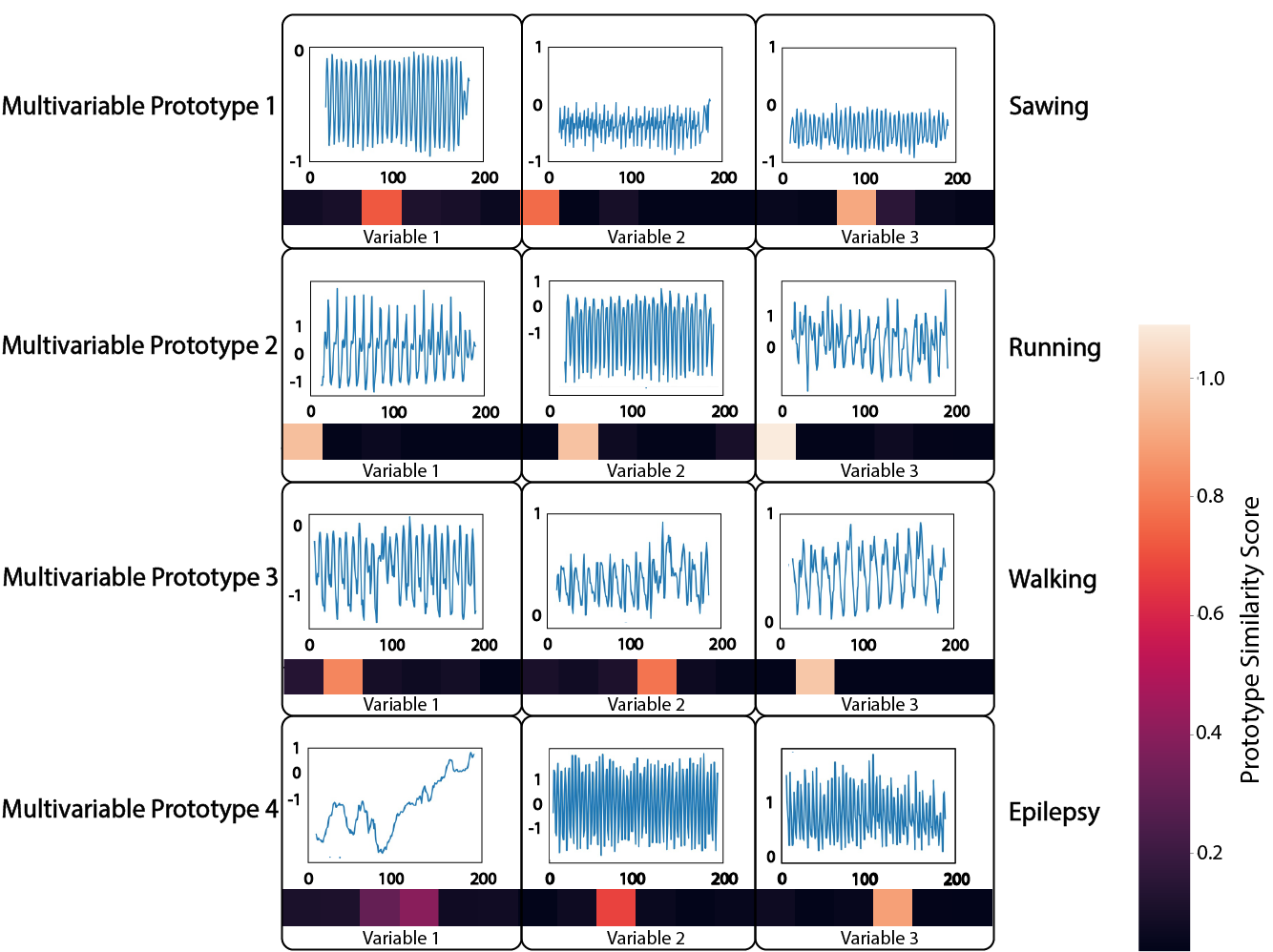
Figure 6: Interpretation of multivariable prototypes for the epilepsy classification task. The multivariable prototype vectors are split into the blocks corresponding to each variable. For each variable block, we represent the single-variable prototype with the highest similarity score by its projection onto the training set.

Multivariable Prototypes

We set the number of multivariable prototypes in this task to 4, based on the number of classes. Visualizations of the learned prototypes are presented in Figure 6. Overall, our interpretations clearly reveal that frequency and amplitude of the signals distinguish the different classes. For example, the sawing class exhibits signals with high frequency but low and uniform amplitudes, consistent with what is expected for a repetitive and controlled movement. The running class, on the other hand shows signals with similarly high frequencies, but larger and varying amplitudes. The slowest activity, walking, is seen to have low frequency oscillations and low amplitudes.

For the running, sawing, and walking classes, the multivariable prototype vectors take the form of one-hot encoded vectors, selecting one prototype from each variable. This reveals that these classes are consistently associated with only one single-variable prototype per variable and that there is no overlap in patterns among these classes, they are completely distinguishable in all variables. For the epilepsy class, on the other hand, there are two entries in the first variable block that are non-zero. This indicates that data points of the epilepsy class show one of two patterns in the first variable, which is verified by the UMAP visualizations in Figure 5. Moreover, we observe that one of these prototypes is also selected in the Sawing class. This reveals these two activities generate similar patterns in the first variable and that the first variable may not be as useful in distinguishing these classes. In this way, we see that our method can provide fine-grained feature importance information, revealing the importance of particular variable with respect to distinguishing individual classes. Notably, the discovery of multiple patterns corresponding to the epilepsy class, as well as the similarities between the sawing and epilepsy classes are a direct result of the inherently interpretable multivariable prototypes introduced in this work.

5 Discussion

Interpretable multivariable time series classification is an essential task for a variety of scientific and industrial applications. In this paper, we have presented a prototype learning based model which allows for the discovery of important patterns at the variable level, as well as easily interpretable rules encoding the relationships between variables that are important for classification. Our method is modular in both its structure and its training procedure, allowing for a large degree of flexibility in handling diverse variable types as well as the opportunity to deploy domain-specific knowledge. On both the simulated and human activity recognition datasets, our framework is able to fully detail the patterns characterizing each class, as well as revealing relationships between different classes and variables.

One limitation of our current work is the need to manually determine the number of single and multivariable prototypes. Future work will examine methods to automate or make this choice more systematic. Another potential area for future work is enhancing the complexity of cross variable patterns that can be represented by our framework. This could potentially be achieved by introducing metric learning in the multivariable representation space, instead of using our current similarity measure. Finally, for more complex or noisy variables, the single variable prototypes alone could be insufficient to identify the meaningful features of the time series. Thus, interpretability could be enhanced by introducing the attention mechanism to the single-variable encoders, potentially providing fine-grained identification of meaningful time points and subsequences within the single-variable prototypes.

We predict that this work will have a net beneficial impact on society. As previously noted, multivariable time series classification problems are ubiquitous in high-impact areas such as medicine and scientific research. In this work, we have provided a method for addressing these problems that explains its predictions. Although nearly all machine learning models can be harmful given biases in their training data, the explanations provided by our method can aid in detecting these biases. Ultimately, we expect that our framework will serve as a powerful tool for researchers in extracting scientific information from large and complex datasets.

References

- [1] Patrick Schäfer and Ulf Leser. Multivariate time series classification with weasel+ muse. arXiv preprint arXiv:1711.11343, 2017.
- [2] Do-Hyung Kwon, Ju-Bong Kim, Ju-Sung Heo, Chan-Myung Kim, and Youn-Hee Han. Time series classification of cryptocurrency price trend based on a recurrent lstm neural network. Journal of Information Processing Systems, 15(3):694–706, 2019.
- [3] Haoyan Xu, Ziheng Duan, Yunsheng Bai, Yida Huang, Anni Ren, Qianru Yu, Qianru Zhang, Yueyang Wang, Xiaoqian Wang, Yizhou Sun, and Wei Wang. Multivariate time series classification with hierarchical variational graph pooling, 2020.
- [4] Joseph Azar, Abdallah Makhoul, and Raphaël Couturier. Using densenet for iot multivariate time series classification. In 2020 IEEE Symposium on Computers and Communications (ISCC), pages 1–6. IEEE, 2020.
- [5] Ashish Gupta, Hari Prabhat Gupta, Bhaskar Biswas, and Tanima Dutta. A divide-and-conquer–based early classification approach for multivariate time series with different sampling rate components in iot. ACM Trans. Internet Things, 1(2), April 2020.
- [6] Bing Zhai, Ignacio Perez-Pozuelo, Emma A. D. Clifton, Joao Palotti, and Yu Guan. Making sense of sleep: Multimodal sleep stage classification in a large, diverse population using movement and cardiac sensing. Proc. ACM Interact. Mob. Wearable Ubiquitous Technol., 4(2), June 2020.
- [7] Değer Ayata, Yusuf Yaslan, and Mustafa E Kamasak. Emotion recognition from multimodal physiological signals for emotion aware healthcare systems. Journal of Medical and Biological Engineering, pages 1–9, 2020.
- [8] Yixiang Dai, Xue Wang, Pengbo Zhang, and Weihang Zhang. Wearable biosensor network enabled multimodal daily-life emotion recognition employing reputation-driven imbalanced fuzzy classification. Measurement, 109:408–424, 2017.
- [9] Joong Hoon Lee, Hannes Gamper, Ivan Tashev, Steven Dong, Siyuan Ma, Jacquelin Remaley, James D. Holbery, and Sang Ho Yoon. Stress monitoring using multimodal bio-sensing headset. In Extended Abstracts of the 2020 CHI Conference on Human Factors in Computing Systems, CHI EA ’20, page 1–7, New York, NY, USA, 2020. Association for Computing Machinery.
- [10] David A Ziegler, Alexander J Simon, Courtney L Gallen, Sasha Skinner, Jacqueline R Janowich, Joshua J Volponi, Camarin E Rolle, Jyoti Mishra, Jack Kornfield, Joaquin A Anguera, et al. Closed-loop digital meditation improves sustained attention in young adults. Nature human behaviour, 3(7):746–757, 2019.
- [11] Jyoti Mishra, Mira Lowenstein, Richard Campusano, Yihan Hu, Juan Diaz-Delgado, Jacqueline Ayyoub, Rajat Jain, and Adam Gazzaley. Closed-loop neurofeedback of alpha synchrony during goal-directed attention. Journal of Neuroscience, 2021.
- [12] Dong Wen, Bingbing Liang, Yanhong Zhou, Hongqian Chen, and Tzyy-Ping Jung. The current research of combining multi-modal brain-computer interfaces with virtual reality. IEEE Journal of Biomedical and Health Informatics, pages 1–1, 2020.
- [13] Reza Abbasi-Asl, Mohammad Keshavarzi, and Dorian Yao Chan. Brain-computer interface in virtual reality. In 2019 9th International IEEE/EMBS Conference on Neural Engineering (NER), pages 1220–1224. IEEE, 2019.
- [14] Yuchae Jung and Yong Ik Yoon. Monitoring senior wellness status using multimodal biosensors. In 2016 International Conference on Big Data and Smart Computing (BigComp), pages 435–438. IEEE, 2016.
- [15] Yuchae Jung and Yong Ik Yoon. Multi-level assessment model for wellness service based on human mental stress level. Multimedia Tools and Applications, 76(9):11305–11317, 2017.
- [16] Dalin Zhang, Lina Yao, Xiang Zhang, Sen Wang, Weitong Chen, Robert Boots, and Boualem Benatallah. Cascade and parallel convolutional recurrent neural networks on eeg-based intention recognition for brain computer interface. In Proceedings of the AAAI Conference on Artificial Intelligence, volume 32, 2018.
- [17] Reza Abbasi-Asl and Bin Yu. Structural compression of convolutional neural networks. arXiv preprint arXiv:1705.07356, 2017.
- [18] Reza Abbasi-Asl, Yuansi Chen, Adam Bloniarz, Michael Oliver, Ben DB Willmore, Jack L Gallant, and Bin Yu. The deeptune framework for modeling and characterizing neurons in visual cortex area v4. bioRxiv, page 465534, 2018.
- [19] W. James Murdoch, Chandan Singh, Karl Kumbier, Reza Abbasi-Asl, and Bin Yu. Definitions, methods, and applications in interpretable machine learning. Proceedings of the National Academy of Sciences, 116(44):22071–22080, 2019.
- [20] Mustafa Gokce Baydogan and George Runger. Learning a symbolic representation for multivariate time series classification. Data Mining and Knowledge Discovery, 29(2):400–422, 2015.
- [21] Josif Grabocka, Martin Wistuba, and Lars Schmidt-Thieme. Fast classification of univariate and multivariate time series through shapelet discovery. Knowledge and information systems, 49(2):429–454, 2016.
- [22] Mohamed F Ghalwash and Zoran Obradovic. Early classification of multivariate temporal observations by extraction of interpretable shapelets. BMC bioinformatics, 13(1):1–12, 2012.
- [23] Wensi Tang, Lu Liu, and Guodong Long. Interpretable time-series classification on few-shot samples. In 2020 International Joint Conference on Neural Networks (IJCNN), pages 1–8. IEEE, 2020.
- [24] Alan H Gee, Diego Garcia-Olano, Joydeep Ghosh, and David Paydarfar. Explaining deep classification of time-series data with learned prototypes. arXiv preprint arXiv:1904.08935, 2019.
- [25] Xuchao Zhang, Yifeng Gao, Jessica Lin, and Chang-Tien Lu. Tapnet: Multivariate time series classification with attentional prototypical network. In The Thirty-Fourth AAAI Conference on Artificial Intelligence, AAAI 2020, The Thirty-Second Innovative Applications of Artificial Intelligence Conference, IAAI 2020, The Tenth AAAI Symposium on Educational Advances in Artificial Intelligence, EAAI 2020, New York, NY, USA, February 7-12, 2020, pages 6845–6852. AAAI Press, 2020.
- [26] Guozhong Li, Byron Choi, Jianliang Xu, Sourav S Bhowmick, Kwok-Pan Chun, and Grace LH Wong. Shapenet: A shapelet-neural network approach for multivariate time series classification. AAAI, 2021.
- [27] Raia Hadsell, Sumit Chopra, and Yann LeCun. Dimensionality reduction by learning an invariant mapping. In 2006 IEEE Computer Society Conference on Computer Vision and Pattern Recognition (CVPR’06), volume 2, pages 1735–1742. IEEE, 2006.
- [28] Adam Paszke, Sam Gross, Francisco Massa, Adam Lerer, James Bradbury, Gregory Chanan, Trevor Killeen, Zeming Lin, Natalia Gimelshein, Luca Antiga, Alban Desmaison, Andreas Kopf, Edward Yang, Zachary DeVito, Martin Raison, Alykhan Tejani, Sasank Chilamkurthy, Benoit Steiner, Lu Fang, Junjie Bai, and Soumith Chintala. Pytorch: An imperative style, high-performance deep learning library. In H. Wallach, H. Larochelle, A. Beygelzimer, F. d'Alché-Buc, E. Fox, and R. Garnett, editors, Advances in Neural Information Processing Systems 32, pages 8024–8035. Curran Associates, Inc., 2019.
- [29] Leland McInnes, John Healy, and James Melville. Umap: Uniform manifold approximation and projection for dimension reduction. arXiv preprint arXiv:1802.03426, 2018.
- [30] Anthony Bagnall, Hoang Anh Dau, Jason Lines, Michael Flynn, James Large, Aaron Bostrom, Paul Southam, and Eamonn Keogh. The uea multivariate time series classification archive, 2018. arXiv preprint arXiv:1811.00075, 2018.
- [31] Jose R Villar, Paula Vergara, Manuel Menéndez, Enrique de la Cal, Víctor M González, and Javier Sedano. Generalized models for the classification of abnormal movements in daily life and its applicability to epilepsy convulsion recognition. International journal of neural systems, 26(06):1650037, 2016.