Reinforcement learning for pursuit and evasion of microswimmers at low Reynolds number

Abstract

We consider a model of two competing microswimming agents engaged in a pursue-evasion task within a low-Reynolds-number environment. Agents can only perform simple maneuvers and sense hydrodynamic disturbances, which provide ambiguous (partial) information about the opponent’s position and motion. We frame the problem as a zero-sum game: The pursuer has to capture the evader in the shortest time, while the evader aims at deferring capture as long as possible. We show that the agents, trained via adversarial reinforcement learning, are able to overcome partial observability by discovering increasingly complex sequences of moves and countermoves that outperform known heuristic strategies and exploit the hydrodynamic environment.

I Introduction

Aquatic organisms can detect moving objects by sensing the induced hydrodynamic disturbances Triantafyllou et al. (2016); Takagi and Hartline (2018); Tuttle et al. (2019). Such an ability is crucial in prey-predator interactions and for navigation, especially in murky or dark waters, as for the blind Mexican cavefish Lloyd et al. (2018). Fishes have developed the lateral line, a mechanosensory system very sensitive to water motions and pressure gradients Montgomery et al. (1997); Bleckmann and Zelick (2009); Kanter and Coombs (2003). Planktonic microorganisms, inhabiting a low-Reynolds-number environment, have antennae and setae to sense hydrodynamic signals produced by predators and preys Kiørboe and Visser (1999); Doall et al. (2002).

Abstracting away from specific mechanisms developed by aquatic organisms, the problem of pursue-evasion in microswimmers guided by hydrodynamic cues poses substantial difficulties rooted in the physics of the ambient medium. At low Reynolds numbers, flow disturbances are generally weak and rich of symmetries Happel and Brenner (2012) leading to ambiguities about the signal source location especially if distant from the receiver Kiørboe and Visser (1999); Takagi and Hartline (2018); Tuttle et al. (2019). Moreover, hydrodynamics has dynamical effects, as the disturbances generated by one microswimmer alter the other motion. Consequently, an agent’s strategy inevitably affects the opponent dynamics and strategies. It is thus crucial to understand how agents’ strategies co-evolve by competing against one another Hein et al. (2020), which necessitates going beyond just escaping from a prescribed pursuit strategy or pursuing a nonresponsive moving target Domenici et al. (2011); Nahin (2012). Which pursuit-evasion strategies can be devised in such dynamic, partially observable environments? How do they coevolve while competing? Can hydrodynamics be exploited and how? How do they compare with strategies based on visual cues?

Here, we formulate the problem of prey-predator microswimmers in a game-theoretic framework Hofbauer and Sigmund (1998), a natural setting to model the emergence of adversarial strategies Hein et al. (2020). As we are interested in the learning and evolution of strategies and not in fine tuning on specific details of the two microswimmers, we choose a simplified hydrodynamics. Inspired by recent applications of multi agent reinforcement Learning (MARL) Sutton and Barto (2018) to hide-and-seek contests Baker et al. (2019); Chen et al. (2020), we explore its use as a general model-free framework for discovering effective chase-and-escape strategies at low Reynolds number. Reinforcement learning (RL) approaches rely on trial and error to improve the quality of the decisions made by an agent – here a microswimmer – and has been already applied in numerical and experimental study of navigation in complex fluid environments Biferale et al. (2019); Alageshan et al. (2020); Reddy et al. (2016); Colabrese et al. (2017); Verma et al. (2018); Mirzakhanloo et al. (2020); Cichos et al. (2020); Qiu et al. (2021); Reddy et al. (2018); Muiños-Landin et al. (2021). We show that RL is able to discover complex strategies, evolving during the different phases of the adversarial learning, and thus depending on the combined training history. The discovered strategies efficiently overcome the limitations imposed by the partial observability. In particular, pursuer strategies are shown to outperform a heuristic baseline policy. Moreover, we show that the main strategies discovered by RL are explainable and for some of them we provide an analytical description, which allows us to rationalize how the pursuer overcomes the difficulties due to partial information.

The material is organized as follows. In Sec. II we present the model. In Sec. III we discuss the basic ideas of reinforcement learning applied to our model and some detail on the implementation. In Sec. IV we present the results, while Sec. V is devoted to discussions and conclusions. Some more technical material is presented in the Appendices and details on the numerical implementation of the reinforcement learning algorithm are discussed in supplementary material .

II Model

II.1 Game theoretic formulation

The basic settings of the game-theoretic formulation of the problem are shown in Figs. 1(a) and 1(b). Agents have a limited maneuverability and partial information on the opponent via hydrodynamic cues, which we choose to be the gradients of the velocity field [Fig. 1(a)]. The two swimming agents play the following zero-sum game [Fig. 1(b)]: They start at distance $R_{0}$ with random heading directions. At each decision time $\tau$ each agent senses the hydrodynamic field and chooses an action (steer left/right or go straight). The pursuer ($p$) aims at reaching the capture distance $R_{c}$ from the evader ($e$) in the shortest possible time, while the latter has to keep the pursuer at bay (at distance $R>R_{c}$). The game terminates either on capture (pursuer wins) or if its duration exceeds a given time $T_{max}$ (evader wins). While playing many games the agents are trained via via reinforcement learning (see Sec. III)

II.2 Modeling the agents

For simplicity, we model the agents as “pusher” discoids in an idealized two-dimensional environment disregarding any effect due to walls or confinements and in the absence of external flows. By swimming, they generate a velocity field modeled as a force dipole moving with speed $v_{\alpha}$ with $\alpha\!=\!e,p$ [Fig. 1(a)]. The force-dipole approximates well the far field of many microorganisms Lauga and Powers (2009). Near-field corrections, depending on details, are not implemented as we are not interested in tuning the model to a specific swimming mechanism, though they can matter in close encounters Ishimoto et al. (2020). Besides self-propulsion each microswimmer is advected and reoriented by the flow generated by the other. Every $\tau$ time units, i.e., at each decision time, agents can steer by imparting a torque, resulting in an angular velocity $\Omega_{\alpha}$. Thus the position $\bm{x}_{\alpha}$ and heading direction $\bm{n}_{\alpha}\!=\!(\cos\theta_{\alpha},\sin\theta_{\alpha})$ evolve as

$$\dot{\bm{x}}_{\alpha} = v_{\alpha}\bm{n}_{\alpha}+\bm{u}^{(\beta)}$$ (1)

$$\dot{\theta}_{\alpha} = \Omega_{\alpha}+\omega^{(\beta)}/2\,,$$ (2)

where $\bm{u}^{(\beta)}(\bm{x})$ and $\omega^{(\beta)}(\bm{x})(=\bm{\nabla}\times\bm{u}^{(\beta)}(\bm{x}))$ are the velocity and vorticity field at position at position $\bm{x}_{\alpha}$, generated by the opponent agent $\beta$ in $\bm{x}_{\beta}$ with heading orientation $\theta_{\beta}$, see Fig. 1c.

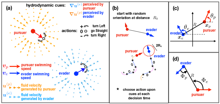
Figure 1: (Color online) Model illustration. (a) Basic elements: The pursuer ($p$, red)/evader ($e$, blue) swims with speed $v_{p/e}$ generating a velocity field $\bm{u}^{(p/e)}$, which drags the other agent and offers a cue to the other agent on the relative position and orientation via its gradients, $\bm{\nabla}\bm{u}^{(p/e)}$. Agents only have a limited control on their heading directions – the actions. (b) Sketch of a game: The game starts with the agents at distance $R_{0}$ and the pursuer/evader goal is to min/maximize the time their distance reaches the capture value $R_{c}$ within a given time horizon. Agents move in the plane, every $\tau$ time-unit they choose to maintain or turn left/right their heading direction on the basis of the cues they receive. (c) Geometry of the problem in a fixed frame of reference with indicated the heading angles. (d) Bearing angle $\Phi_{e/p}$ corresponding to the angular position of an agent with respect to the heading direction of its opponent.

As detailed in Appendix A, we can write $\bm{u}^{(\beta)}(\bm{x})\!=\!(\partial_{y},-\partial_{x})\Psi(\bm{x}\!-\!\bm{x}_{\beta};\theta_{\beta})$, with the stream function $\Psi=\nicefrac{{D_{\beta}}}{{2}}\sin(2\phi-2\theta_{\beta})$, where $\bm{x}-\bm{x}_{\beta}=|\bm{x}-\bm{x}_{\beta}|(\cos\phi,\sin\phi)$ and $D_{\beta}$ denotes the dipole intensity of agent $\beta$. We consider $D_{\beta}>0$, i.e., pusher like microswimmers Lauga and Powers (2009). The velocity in Eq. (1) is then obtained by deriving the stream function in $\bm{x}=\bm{x}_{\alpha}$, corresponding to $\phi=\phi_{\alpha}$ [see Fig. 5(a) for the notation on the angles with respect to a fixed frame of reference]. While the vorticity in Eq. (2) is $\omega^{(\beta)}=2D_{\beta}/R^{2}\sin(2\phi_{\alpha}-2\theta_{\beta})=2D_{\beta}/R^{2}\sin(2\phi_{\beta}-2\theta_{\beta})$, with $R=|\bm{x}_{\alpha}-\bm{x}_{\beta}|$ and the second equality stemming from $\phi_{\beta}=\phi_{\alpha}+\pi$ [Fig. 5(a)].

II.3 Modeling the hydrodynamic cues

As already discussed, we assume an agent can only sense the gradients of the velocity field generated by its opponent, similarly to what copepods do with sensory setae Kiørboe and Visser (1999). Since agents have no notion of an external frame of reference we assume that they perceive the gradients in their own frame of reference, i.e., projected along the angents’ swimming direction. In this frame of reference the three independent components (vorticity and longitudinal and shear strain) of the velocity gradients read

$$\omega^{(\beta)}\! = \partial_{x}u^{(\beta)}_{y}\!-\!\partial_{y}u^{(\beta)}_{x}=\frac{2D_{\beta}}{R^{2}}\sin(2\Phi_{\beta}-2\Theta_{\beta})$$ (3)

$$\mathcal{L}^{(\beta)}\! = \partial_{x}u^{(\beta)}_{x}\!=\!-\partial_{y}u^{(\beta)}_{y}=-\frac{D_{\beta}}{R^{2}}\cos(4\Phi_{\beta}\!-\!2\Theta_{\beta})$$ (4)

$$\mathcal{S}^{(\beta)}\! = \frac{1}{2}(\partial_{x}u^{(\beta)}_{y}\!+\!\partial_{y}u^{(\beta)}_{x})\!=\!-\frac{D_{\beta}}{R^{2}}\sin(4\Phi_{\beta}\!-\!2\Theta_{\beta})\,.$$ (5)

They depend on agents’ distance ($R$), relative heading $\Theta_{\beta}\!=\!\theta_{\beta}-\theta_{\alpha}$ [see Fig. 5(b)] and angular position of $\beta$ with respect the heading direction of $\alpha$, $\Phi_{\beta}\!=\!\phi_{\beta}-\theta_{\alpha}$, i.e., the bearing angle [Fig. 1(d)], as called in the pursuit-evasion-games language Nahin (2012).

In general, gradients are symmetric with respect to parity, i.e., to the combined transformation $\Theta_{\beta}\!\to\!\Theta_{\beta}+\pi$ and $\Phi_{\beta}\!\to\!\Phi_{\beta}+\pi$. The force dipole case is even more degenerate as, owing to the fore-aft symmetry, either of the two transformations leaves the gradients unchanged, due to the nematic nature of dipoles. Such symmetries result in ambiguities in the identification of the position and orientation of the opponent, akin to the $180^{o}$ ambiguity in fish hearing Wubbels and Schellart (1997). Memory of past detections and/or multiple hydrodynamical cues can, in principle, mitigate such ambiguities which, however, typically persist at large distances Sichert et al. (2009); Triantafyllou et al. (2016); Takagi and Hartline (2018). In spite of its simplicity the model is thus rich enough to represent the typical observability limitation inherent to organisms that can only perceive the gradients of the velocity field.

III Learning to pursue and evade through reinforcement

To set up a learning framework, we need to identify: a set of observations, $o$, that an agent perceives and uses to infer the opponent’s state; the actions, $a$, through which it can implement its strategy; and the rewards, $r$, to evaluate its actions. The learning task here is to find an optimal reactive policy, $\pi^{*}(a|o)$, that associates actions to observations in order to maximize the expected cumulative rewards. In our setting, the environmental state (relative position and heading) is only partially observable through the velocity gradientsJaakkola et al. (1995). The actions $a\in{\cal A}\!=\!\{0,+,-\}$ [Fig. 1(a)] correspond to the three angular velocities $\Omega_{\alpha}\!=\!0,+\varpi_{\alpha},-\varpi_{\alpha}$ agent $\alpha$ can choose to control its orientation. Once actions are taken, the agents evolve for a time $\tau$ with the dynamics (1) and (2) and a reward is issued. In this zero-sum game, the currency is the elapsing time: The pursuer/evader receives a reward $r\!=\!\mp 1$ at the end of each decision time. After each action, the agents update their policy by combining past and new information with the issued reward. In the new state, gradients are sensed again, new actions are taken and rewards received; the cycle repeats itself until the terminal state is achieved, with either the pursuer (if $R\leq R_{c}$) or the evader winning (if the game duration exceeds $T_{max}$). The total return accumulated by the pursuer/evader in an episode is therefore $\mp T$ where $T$ is the duration of the episode itself.

III.1 Reinforcement Learning algorithm

Among the many approaches to MARL we adopt a natural actor-critic architecture (see Bhatnagar et al. (2009); Grondman et al. (2012) and supplementary material Note (1) for details) because of its theoretical guarantees and connection with evolutionary game theory Hennes et al. (2019); Hofbauer and Sigmund (1998). In this class of algorithms, locally optimal solutions are sought by means of stochastic gradient ascent in policy space. Natural gradients are used, by virtue of their covariance with respect to the metric defined by the Fisher information Amari (1998). Real organisms process the environmental cues with their nervous system that encodes the policy, e.g., in fishes dedicated neurons control escape responses Eaton et al. (2001). Such neural encoding can be emulated by artificial neural networks Arulkumaran et al. (2017). Here, in the interest of explainability, we opted for an explicit parametrization of the policy in terms of few selected features of the observations. Dropping the agent indices for simplicity, we set

$$\pi(a|o)=\frac{\exp(\mathbfcal{F}(o)\cdot\bm{\xi}_{a})}{\sum_{a^{\prime}}\exp({\mathbfcal{F}(o)\cdot\bm{\xi}_{a^{\prime}}})}\,,$$

where $a,a^{\prime}\in\mathcal{A}$, $\mathbfcal{F}(o)$ are features that encode the observations $o$, and $\bm{\xi}_{a}$ the learning parameters.

By combining the velocity-gradient components, we chose to extract the following observables ($o$) (see Appendix B): the vorticity $\omega$; a proxy for the agents’ distance, $\hat{R}\propto 1/R^{2}$; and a linear combination of heading and bearing angle $\gamma=4\Phi\!-\!2\Theta$. As features, $\mathbfcal{F}(o)$, we used the raw observables $\omega$ and $\hat{R}$, and the first and second harmonics of angle $\gamma$. To encode for the heading direction, we include some short-term memory by combining a few past observations. As discussed in Appendix B, exploratory studies with more features did not give qualitatively different results from the minimal setting described above. Moreover, eliminating memory yields the same strategies, which indicates that a more sophisticated exploitation of memory is needed.

III.2 Training scheme

To better interpret the evolution of strategies and counter-strategies, we organized learning in phases (each made of $M\!=\!5\times 10^{3}$ episodes) where agents alternately improve their policies. Assuming no prior knowledge, agents start their training with a random policy, $\pi(a|o)\!=\!1/|\mathcal{A}|\!=\!1/3$ for all $o$. At first, the pursuer learns with the evader’s policy frozen, and then the evader learns against the pursuer policy from the previous phase, and so on. Episodes start with agents at a distance $R_{0}\!=\!1$ and random heading directions, and end either on capture ($R\!\leq\!R_{c}\!=\!0.05R_{0}$) or when time exceeds the cap $T_{max}\!=\!50T_{0}$, where $T_{0}\!=\!R_{0}/v_{e}$ is estimated in terms of the evader speed and initial distance. We fixed the evader speed at $v_{e}\!=\!0.1$ and angular velocity $\varpi_{e}\!=\!3$. For the pursuer, we chose $(v_{p},\varpi_{p})\!=\!(0.15,4.5)$ which gives a slight speed advantage maintaining the same steering ability (same curvature radius $v_{p}/\varpi_{p}\!=\!v_{e}/\varpi_{e}$). The intensity of the force dipole is taken to be equal for both agents $D_{p}=D_{e}=0.03$. With this choice hydrodynamic velocity dominates over swimming at distances $R\lesssim R_{0}$. The decision time is $\tau\!=\!0.01T_{0}$ for both agents.

IV Results

Our main results are summarized in Fig. 2: Figure 2(a) shows the running average of normalized game duration $T/T_{max}$ in the first six learning phases for three independent learning experiments; Figs. 2(b)-2(g) and Figs. 2(h)-2(m) display some representative examples of pursuer and evader winning strategies, respectively. Cycles 1 and 2 are quite reproducible: The pursuer discovers ways to rapidly catch the evader which, in turn, finds ways to counteract. Conversely, cycles 3-6 are characterized by a higher variability: Agents seem to acquire and lose good policies also within their own learning turn, and we see cases (run1 in Fig. 2a) in which the evader eventually dominates the game. We hypothesize that such variability arises from a combination of insufficient hyperparameters tuning and/or subtle instabilities in the learning algorithm. Notwithstanding these limitations, many aspects of the learned strategies are reproducible and, to some extent, physically explainable as discussed below. The effect of a variation of the parameters and the addition of rotational noise is discussed in Sec. II of supplementary material Note (1).

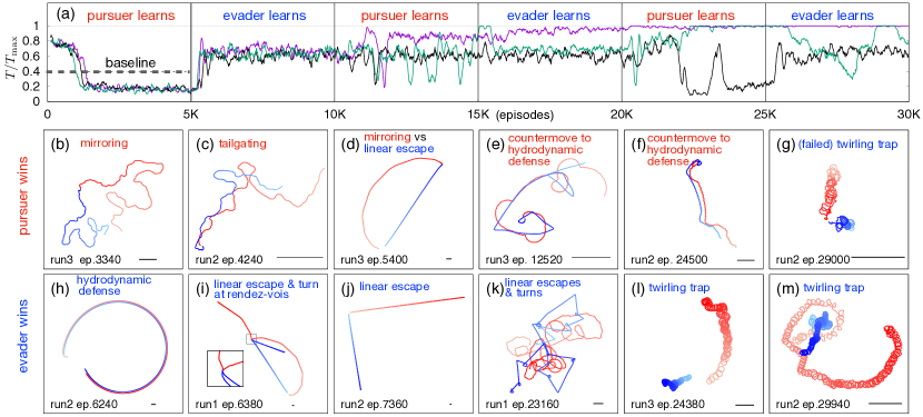
Figure 2: (Color online) Co-evolving strategies in the first six training cycles. (a) Running average (over 100 episodes) of normalized episode duration $T/T_{max}$ for three realizations of learning: run1, run2 and 3 (purple, green and black curves). The dashed horizontal gray line represents a heuristic baseline value as discussed in Sec. IV.1.1. [(b)-(g)] Winning pursuit strategies: (b) mirroring, (c) tailgating, (d) mirroring vs linear escape with a rendez-vous, [(e) and (f)] tailgating with countermoves to hydrodynamic defense, and (g) failing twirling on mirroring. [(h)-(m)] Winning evasion strategies: (h) hydrodynamic defense, (i) linear escape with turn and hydrodynamic collision at rendez-vous, (j) linear escape against mirroring, (k) linear escapes and turns inducing pursuer switches between mirroring and tailgating at distance, and [(l) and (m)] twirling trap. Red/blue denotes pursuer/evader trajectories, time runs from lighter to darker color (apparent close encounters actually take place at different times); run/episode labeled on each panel; the bottom-right bar displays the unit length.

IV.1 Pursuit strategies: Mirroring and tailgating

In its first learning phase, the evader executes a random cue-insensitive policy, while the predator learns to pursue its prey either “mirroring” its actions [Fig. 2(b)] or “tailgating” it [Fig. 2(c)]. When the pursuer approaches the evader, a switch between the two strategies can sometimes be observed presumably due to hydrodynamical effects overcoming self-swimming at these distances combined to evader turning [Fig. 3]. Close inspection reveals that the pursuer orchestrates its actions in such a way to enforce over time specific relations (linked to the hydrodynamical cues as discussed in Appendix C) between the bearing angles, namely $\Phi_{e}\!=\!-\Phi_{p}$ for mirroring and $\Phi_{e}\!=\!-\Phi_{p}+\pi$ for tailgating [Fig. 3(a)]. Due to the aforementioned $180^{o}$ ambiguities, the pursuer cannot discern mirroring and tailgating just on the basis of instantaneous hydrodynamical cues: The strategy chosen depends on initial conditions and hydrodynamic interactions [as, e.g., in Fig. 3(b)]. The two strategies emerge from the same policy in response to partial observability and can be analytically described, as detailed in Appendix C and briefly summarized in the following. On neglecting hydrodynamical interactions in Eqs. (1) and (2), we can derive the equations for the separation and bearing angle Belkhouche et al. (2007). By imposing that the pursuer follows either mirroring or tailgating, such equations read

$$\dot{R} = -(v_{p}\pm v_{e})\cos\Phi_{e}$$ (6)

$$\dot{\Phi}_{e} = \Omega_{e}-R^{-1}\;(v_{p}\mp v_{e})\sin\Phi_{e}\,,$$ (7)

with $\pm$ for mirroring/tailgating. Equation (6) shows that tailgating is doomed to fail when $v_{p}=v_{e}$ as $\dot{R}=0$, while for $v_{p}>v_{e}$ it becomes an efficient strategy as the dynamics (7) leads to $\Phi_{e}\!\to\!0$ for small enough distances, and (6) implies $\dot{R}<0$. Mirroring remains effective also for $v_{p}\!=\!v_{e}$ (and $\Omega_{e}$ random) as it essentially maps the pursue into a first hitting problem for a random search with dimensionality reduction Adam and Delbrück (1968). Tests with RL and the full dynamics [Eqs. (1) and (2)] for $v_{p}\!=\!v_{e}$ confirmed the scenario.

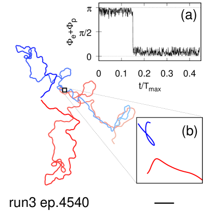
Figure 3: (Color online) Switching between tailgating to mirroring. Inset (a): Sum of bearing angles $\Phi_{e}\!+\!\Phi_{p}$ vs normalized time. Proximity and evader turning [inset (b)] triggers the switch $\Phi_{e}\!+\!\Phi_{p}\!\approx\!\pi\!\to\!0$ (tailgating $\to$ mirroring) at $t/T_{max}\!\approx\!0.15$.

IV.1.1 Comparison with a heuristic strategy based on visual cues adapted to partial information

It is interesting to compare the pursuit policies discovered by RL against well-established visual pursuit strategies based on the knowledge of the line of sight with the target Nahin (2012); Belkhouche et al. (2007). Mirroring bears some similarities with parallel navigation, where the line-of-sight direction is kept constant with respect to an inertial frame of reference, a strategy that appears to be applied by dragonflies Olberg et al. (2000). Tailgating resembles pure pursuit, where heading is constantly directed toward the line of sight (zero bearing angle), as bats or some fishes appear to do Chiu et al. (2010); Lanchester and Mark (1975). Such strategies cannot be directly implemented here because of the $180^{o}$ ambiguities inherent to perceiving only the gradients. However, we can introduce a heuristic strategy in the form of a randomized pure pursuit: The pursuer heads either toward the evader ($\Phi_{e}\!=\!0$) or to its “image” ($\Phi_{e}\!=\!\pi$) with equal probability with some persistency in time. As a limiting case, it could randomly choose its target once for all at the beginning, in which case it is bound to fail half of the times so that $\langle T\rangle/T_{max}>1/2$; however, the pursuer may instead randomly choose either targets every $N_{p}$ decision times (we call $N_{p}$ persistency). By scanning $\langle T\rangle/T_{max}$ as a function of $N_{p}$, at $N_{p}\approx 400$ we numerically found the minimum $\langle T\rangle/T_{max}\approx 0.4$ [see Fig. 4 and dashed line in Fig. 2(a)] which is slightly more than twice the value obtained with the mirroring-tailgating strategy. The policy discovered by RL clearly outperforms the randomized pure pursuit offering a more efficient way to overcome the ambiguities due to the partial information provided by the hydrodynamic cues.

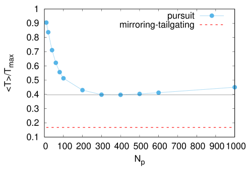
Figure 4: (Color online) $\langle T\rangle/T_{max}$ as a function of the persistency $N_{p}$ (circles) of the randomized pure pursuit strategy described in text. The black line shows the normalized episode duration for the optimal $N_{p}$, while the red dashed line shows the average value obtained with the mirroring-tailgating strategy obtained from Fig. 2(a).

IV.2 Evader strategies: Hydrodynamic defense and linear flights

In its training phase, the evader learns to contrast mirroring and tailgating. As for the latter, it finds a way to exploit hydrodynamics [Fig. 2(h)]. In many episodes of this kind, the pursuer approaches its opponent from behind with small bearing angle (tailgating). The evader reacts by placing itself in a position relative to its predator such that its backward push cancels the speed advantage of the pursuer and keeps it at bay at a fixed distance (supplementary movie1 displays the pursuer’s trajectory in the frame of reference of the evader). In principle, near-field corrections to the force dipole could modify the hydrodynamic defense, and it would be interesting to explore this aspect when focusing on specific microswimmers. Another strategy adopted by the evader takes the form of an almost linear escape trajectory [Figs. 2(i) and 2(j)]. As shown in Fig. 2(d), this is not always successful as, via mirroring, the pursuer can intercept the evader to a rendezvous point by performing a long smooth arc. Such arcs correspond to adjusting the axis of mirroring in the course of time. However, either by making such rendezvous point very far [Fig. 2(j)] or by exploiting hydrodynamics and turns on close encounters [Fig. 2(i)], the evader can consistently make its evasion strategies quite efficient.

IV.3 Refining strategies

As training proceeds both agents learn more complex strategies in response to the ones described above. We now briefly discuss some examples that stand out because of their repeated occurrence and explainability. Interestingly, the pursuer discovers different ways to contrast the hydrodynamic defense of its opponent [Figs. 2(e) and (f), see also supplementary movie2]. Remarkably, the evader learns to devise diverse winning manouvers as in Fig. 2(k), which consist in linear escapes and turnings which make the predator switching from mirroring to tailgating before capture (see supplementary movie3). The evader also discovers that twirling can trap the pursuer [Fig. 2(l) and 2(m)] in a looping motion induced by its own mirroring-tailgating strategy. Trapping is not always successful though [Fig. 2(g)]. With small variations, the basic strategic patterns discussed above are found also with different parameter choices and will be reported elsewhere.

V Conclusions

In this study, we have shown how microswimmers can discover complex strategies to pursue and evade from each other, even if endowed with limited maneuvering ability and inherently equivocal information about their relative position and orientation. Our study presents a novel game-theoretic approach to pursuit and evasion in an aquatic microenvironment. We expect it to spur further research on the use of reinforcement learning algorithms to rationalize observed prey-predator interactions in more general contexts Hein et al. (2020). Owing to the simplicity of our model we have been able to analytically describe some of the strategies discovered by RL and show why they are effective in overcoming partial observability: For instance, mirroring and tailgating allow to reduce the dimensionality of the search by mapping the search into a first hitting problem. In this respect it would be interesting to study a three dimensional version of the problem to understand which dimensionality reduction could emerge in that case and if it can be still reduced to a one-dimensional hitting time problem.

The present model can be easily generalized to ellipsoidal swimmers, by adding to Eq. (2) rotation by the strain-rate tensor. It can also be extended to “pullers” as well as to other specific microswimmers by including the appropriate near-field hydrodynamics. Indeed while, e.g., mirroring and tailgating are expected to maintain their efficiency in the far field, the pursuer policy may need some refinement in the near-field in order to account for more complex hydrodynamic interactions and near-field corrections would also modify the response of the evader (e.g., the kind of hydrodynamic defense it can develop). With suitable modifications of the hydrodynamics, the approach that we developed here can be used to train underwater robots which can sense the hydrodynamic fields with bioinspired mechanosensorsKottapalli et al. (2015); Free et al. (2020) and thus accomplish complex tasks – for instance, artificial fishes that imitate escape responses Marchese et al. (2014). Here we did not discuss the effect of external flows and boundaries. Preliminary results in a circular arena confirm that the agents can learn to exploit hydrodynamics to perform their pursue/evasion tasks in spite of the confounding cues and complex dynamics arising from the presence of the walls.

Exciting and formidable challenges still lie ahead, and among them stands out the emergence of collective pursue strategies like wolf-packing, and collective escape responses such as hydrodynamic cloaking Mirzakhanloo et al. (2020).

Appendix A Force-dipole hydrodynamic fields

As described in Sec. II.2, we model the agents as two swimming discoids which generate a force dipole, in the sequel we detail the hydrodynamic fields, which enter the dynamics of the agents [see Eqs. (1) and (2)], generated by a force dipole in two dimensions.

We start considering a Stokeslet, i.e., the fundamental solution of the Stokes equation for a point force, $\bm{F}=F\bm{n}$, which, for the sake of simplicity, we locate in the origin, and thus solving the equation

$$\nu\Delta\bm{u}-\bm{\nabla}p=\bm{F}\delta(\bm{x})\,,$$ (8)

where $\bm{u}$ and $p$ are the velocity and pressure field, and $\nu$ the fluid viscosity. The fundamental solution to Eq. (8) in two dimensions is

$$u_{i}(\bm{x})=G_{ij}(\bm{x})F_{j}\,,$$ (9)

where $G$ is the Green function:

$$G_{ij}(\bm{x})=\frac{1}{4\pi\nu}\left[-\delta_{ij}\ln\left(\frac{|\bm{x}|}{L}\right)+\frac{x_{i}x_{j}}{|\bm{x}|^{2}}\right]$$ (10)

with $L$ being an arbitrary length. The pressure field takes the form $p(\bm{x})=\bm{F}\cdot\bm{x}/(4\pi|\bm{x}|^{3})+p_{\infty}$, with $p_{\infty}$ a constant.

Considering two point forces $\bm{F}^{\pm}=\pm F\bm{n}$ located in $\bm{x}^{\pm}=\pm\epsilon\bm{n}$, with $\epsilon\ll 1$ and using Eq. (9), we can express the velocity field generated by this couple as

$$\bm{u}(\bm{x})=G_{ij}(\bm{x}-\bm{x}^{+})F^{+}_{j}+G_{ij}(\bm{x}-\bm{x}^{+})F^{-}_{j}\simeq-2Fn_{k}\partial_{k}G_{ij}(\bm{x})n_{j}$$ (11)

where $F^{+}_{i}=-F^{-}_{i}=Fn_{i}$ and we retained only the first order, to obtain an expression which well approximates the velocity field for large distances $|\bm{x}|\gg\epsilon$. Working out the algebra yields:

$$\bm{u}(\bm{x})=\frac{D}{|\bm{x}|}\left[2\left(\frac{\bm{n}\cdot\bm{x}}{|\bm{x}|}\right)^{2}-1\right]\frac{\bm{x}}{|\bm{x}|}=\frac{D}{|\bm{x}|}\cos(2\phi-2\theta)(\cos\phi,\sin\phi)$$ (12)

where $D=F\epsilon/(2\pi\nu)$ measures the dipole intensity ($D>0$ corresponding to pushers and $D<0$ to pullers Lauga and Powers (2009)) and, in the second equality, $\bm{x}=|\bm{x}|(\cos\phi,\sin\phi)$ and $\bm{n}=\bm{n}(\theta)=(\cos\theta,\sin\theta)$. Notice that the velocity (12) can equivalently be derived as $\bm{u}=(\partial_{y}\Psi,-\partial_{x}\Psi)$ where $\Psi$ is the stream function which can be written as

$$\Psi(\bm{x})=\frac{D}{2}\sin(2\phi-2\theta)\,.$$ (13)

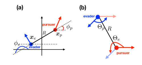
Figure 5: (Color online) Description of relevant angles entering the agent dynamics. (a) In a fixed frame of reference it is shown the angular position of the pursuer $\phi_{p}$ and of the evader $\phi_{e}$, heading angles are shown in Fig. 1(b). (b) We show the relative heading angles $\Theta_{e}=\theta_{e}-\theta_{p}$ and $\Theta_{p}=\theta_{p}-\theta_{e}$, needed together with the bearing angles [Fig. 1(d)] to express the velocity gradients in the pursuer and evader frame of reference, respectively.

The velocity field due to agent $\beta$ and advecting agent $\alpha$ [see Eq. (1] is simply obtained from Eq. (12) substituting $\phi=\phi_{\alpha}$ and $\theta=\theta_{\beta}$, where $\theta_{\beta}$ are the heading directions shown in Fig. 1(c), and $\phi_{\alpha}$ the angular position with respect to a fixed frame of reference shown in Fig. 5(a). The vorticity field due to agent $\beta$ and rotating the heading orientation $\theta_{\alpha}$ of agent $\alpha$ instead can be easily derived to be:

$$\omega^{(\beta)}=\frac{2D_{\beta}}{R^{2}}\sin(2\phi_{\alpha}-2\theta_{\beta})=\frac{2D_{\beta}}{R^{2}}\sin(2\phi_{\beta}-2\theta_{\beta})$$ (14)

with $R=|\bm{x}_{\alpha}-\bm{x}_{\beta}|$ and the second equality stemming from $\phi_{\beta}=\phi_{\alpha}+\pi$ [Fig. 5(a)].

Appendix B Choice of observables and features

Equations (3)-(5) express the gradients in the frame of reference the observing agent. The three independent components of the gradients $\omega,\mathcal{L}$ and $\mathcal{S}$ can be mapped one to one onto the space of the following quantities $o=\{\omega,\hat{R},\gamma\}$, which we assume are observables. Here, $\omega$ is the vorticity itself, which combines information about the agent distance and about $\sin(2\Phi-2\Theta)$. The other two quantities can easily obtained combining the expression of the longitudinal and shear strain, as $\hat{R}\!=\!(\mathcal{L}^{2}\!+\!\mathcal{S}^{2})^{1/2}\propto 1/R^{2}$ and $\gamma=\mathrm{arctan2}(\mathcal{S}/\mathcal{L})$. The observations $o$ offer partial information about the other agent due to the $180^{o}$ ambiguities in $\Theta$ and $\Phi$ discussed in Sec. II.3. The policy is parameterized by the features $\mathcal{F}(o)$, i.e., functions of the observables. Notice that even if $o$ was precisely identifying the reciprocal position of the agents, in order to have access to the full space of possible policies, the features should be chosen as a complete functional basis of the observation, which is not practicable if not using deep reinforcement learning techniques, an option that we did not adopt to have a better understanding of the discovered policies. So we encode the observations $o$ by using a set of only $N_{F}$ features and, consequently, the agents must decide their actions in condition of partial observability Sutton and Barto (2018); Jaakkola et al. (1995)).

We tested different choices of the features and the results presented in Fig. 2 correspond to the choice of the $N_{F}=13$ features summarized in Table 1.

$\mathcal{F}_{1}(o_{t})=\hat{R}(t)$
$\mathcal{F}_{2}(o_{t})=\sin(\gamma(t))$
$\mathcal{F}_{3}(o_{t})=\cos(\gamma(t))$
$\mathcal{F}_{4}(o_{t})=\sin(2\,\gamma(t))$
$\mathcal{F}_{5}(o_{t})=\cos(2\,\gamma(t))$
$\mathcal{F}_{6}(o_{t})=\omega(t)$
$\mathcal{F}_{i}(o_{t})=(1-\mu)\;\mathcal{F}_{i}(t-\tau)+\mu\;\mathcal{F}_{i-6}(t-\tau)\quad\mathrm{for}\quad i=7,12$
$\mathcal{F}_{13}(o_{t})=1$

Table 1: Implemented Features. Note that features $7-12$ provide some memory of the values of the previous features, in the implementation we chose $\mu=0.3$ to retain some memory about the last $2-4$ past observations approximately).

While the first six features are clearly related to the information that can be extracted from gradients, the features $i=7,12$ are introduced to provide the agents with some memory, which may mitigate some of the aforementioned ambiguities. Finally, the $13^{th}$ feature is unrelated to the gradients and it is chosen to allow the agents to adopt strategies independent of the percepts.

We remark that the mirroring and tailgating strategies discussed in Sec. IV.1 can be obtained also removing memory (i.e., features from $7$ to $12$) while they seem to crucially depend on features 4 and 5 which, as explained before, are derived from the strain components Eqs. (4) and (5). These two features are clearly related to mirroring and tailgating strategies (see also Appendix C). Indeed, by removing them, such basic strategies are lost. In order to assess the robustness of our results, we tested the algorithm with different choices of features. Specifically, we tried using powers (both positive and negative) of $\hat{R}$, higher harmonics of $\gamma$ and various products of the percepts. For instance, we tried to add the following features $\cos(3\gamma)$, $\sin(4\gamma)$, $\cos(3\gamma)$, $\cos(4\gamma)$, $\omega\cos(\gamma)/\hat{R}$, $\omega\sin(\gamma)/\hat{R}$, $\omega\sin(2\gamma)/\hat{R}$, $\omega\cos(2\gamma)/\hat{R}$, $\hat{R}\cos(\gamma)$, $\hat{R}\sin(\gamma)$, $\hat{R}\sin(2\gamma)$, $\hat{R}\cos(2\gamma)$, $\hat{R}\sin(3\gamma)$, $\hat{R}\cos(3\gamma)$, $|\omega|$ and $\omega/\hat{R}$. In a separate batch of tests, we tried to use $\hat{R}^{2}$ and $\log\hat{R}$. While it cannot be excluded that we did miss a specific combination of features or that we did not run enough tests, the strategies emerging from these additional trials were qualitative equivalent to those presented in Fig. 2.

Appendix C Analytical description of mirroring and tailgating strategies

In this Appendix we discuss the mirroring [Fig. 2(b)] and tailgating ([Fig. 2(c)] strategies and derive Eqs. (6) and (7).

First we recall the definitions [see also Figs. 1(c) and 1(d) and Figs. 5(a) and 5(b)] of the relative heading angle $\Theta_{e}=\theta_{e}-\theta_{p}$, bearing angle from the point of view of the pursuer, $\Phi_{e}=\phi_{e}-\theta_{p}$, and of the evader, $\Phi_{p}=\phi_{p}-\theta_{e}$; moreover, we recall that $\phi_{e}=\phi_{p}+\pi$ [see Fig. 5(a)]. As discussed in Sec. IV.1 in these strategies the pursuer chooses its actions in such a way to approximatively keep the following relations between the two bearing angles:

$$\begin{cases}\Phi_{p}=-\Phi_{e}\phantom{+\pi}\;\;\qquad\mathrm{Mirroring}\\ \Phi_{p}=-\Phi_{e}+\pi\qquad\mathrm{Tailgating}\,.\end{cases}$$ (15)

As discussed in Appendix B, one of the key observables available to the pursuer is the angle $2\Phi_{e}-\Theta_{e}$, with simple algebra one can recognize that

$$2\Phi_{e}-\Theta_{e}=\Phi_{p}+\Phi_{e}-\pi\,,$$ (16)

so that we can re-express (15) as

$$2\Phi_{e}-\Theta_{e}=\Gamma_{\pm}\mod 2\pi$$ (17)

or equivalently, in the laboratory frame of reference

$$\theta_{p}+\theta_{e}=2\phi_{e}-\Gamma_{\pm}\,,$$ (18)

with $\Gamma_{+}=\pi$ for mirroring and $\Gamma_{-}=0$ for tailgating respectively. Note that $(\theta_{p}+\theta_{e})/2$ identifies (for $v_{p}=v_{e}$ exactly, and otherwise approximatively) the axis of symmetry with respect to which the pursuer trajectory mirrors the one of the evader.

Notice that, at least in the absence of memory, $\Gamma_{\pm}$ cannot be discriminated from observing gradients alone due to the fore-aft symmetry of the swimming dipole. Therefore, depending on the initial condition the agent will pick one of two strategies. Unless the pursuer can resolve the aforementioned ambiguity, it must learn both strategies or neither. In the actual hydrodynamic simulations we have added memory effects (see features $\mathcal{F}_{i}$ for $i=7,12$ in Table 1) to possibly allow the agents to break the fore-aft symmetry in observations. Though tests in the absence of memory suggest that the way memory was implemented is likely not sufficient to eliminate such ambiguities. Anyway, we will ignore possible memory effects in the following.

In order to explore the basic features of such strategies we will neglect also the hydrodynamic effects (i.e., we will not consider the effects on the pursuer due to the velocity field induced by the evader) meaning that we approximate Eqs. (1) and (2) as

$$\dot{\bm{x}}_{\alpha} = v_{\alpha}\bm{n}(\theta_{\alpha})$$ (19)

$$\dot{\theta}_{\alpha} = \Omega_{\alpha}\,.$$ (20)

Moreover, while for the evading agent we assume the dynamics as given by Eqs. (19) and (20) with $\Omega_{e}$ chosen random among the values $0,\pm\varpi_{e}$, as in Ref. Belkhouche et al. (2007) for the pursuer we enforce the constraint (18) exactly. It is worth underlying that the above kinematic equations remain valid also for $\Omega_{e}$ non random. Then we can derive – in polar coordinates $R=|\bm{x}_{e}-\bm{x}_{p}|$ and $\Phi_{e}$ – the motion of the pursuer in the pursuer frame of reference.

Computing $\dot{R}$:  In order to compute $\dot{R}$, we have to project both velocities on the direction ($\phi_{e}$) connecting the two agents. We can use Eqs. (17)-(15) (i.e., we can either project velocities onto the pursuer to evader direction of motion or compute $\dot{R}$ with the chain rule). This procedure leads to $\dot{R}=v_{e}\cos(\theta_{e}-\phi_{e})-v_{p}\cos(\theta_{p}-\phi_{e})=v_{e}\cos(\Phi_{e}-\Gamma_{\pm})-v_{p}\cos(\Phi_{e})$, and thus to $\dot{R}=-(v_{p}\pm v_{e})\cos(\Phi_{e})$.

Computing $\dot{\Phi}_{e}$:  Let us now focus on $\dot{\Phi}_{e}$. By using Eq. (18) and that $\dot{\theta}_{e}=\Omega_{e}$ (being $\Omega_{e}$ the angular velocity selected by the pursuer), we can deduce that $\dot{\theta}_{p}=2\dot{\phi}_{e}-\Omega_{e}$ which implies that

$$\dot{\Phi}_{e}=-\dot{\phi}_{e}+\Omega_{e}$$ (21)

On the other hand, a direct computation yields

$$\dot{\phi}_{e}=\frac{1}{R}[v_{e}\sin(\theta_{e}-\phi_{e})-v_{p}\sin(\theta_{p}-\phi_{p})]\,.$$ (22)

Now using Eqs. (21) and (22) and noticing that $\theta_{e}-\phi_{e}=\phi_{e}-\theta_{p}-\Gamma_{\pm}=\Phi_{e}-\Gamma_{\pm}$ from (18), we can deduce that

$$\dot{\Phi}_{e}=\Omega_{e}-\frac{1}{R}[v_{e}\sin(\Phi_{e}-\Gamma_{\pm})+v_{p}\sin(\Phi_{e})]=\Omega_{e}-\frac{1}{R}(v_{p}\mp v_{e})\sin(\Phi_{e})\,.$$ (23)

We can then summarize the previous results in the set of equations

$$\begin{dcases}\dot{R}&=-(v_{p}\pm v_{e})\cos(\Phi_{e})\\ \dot{\Phi}_{e}&=\Omega_{e}-\frac{1}{R}(v_{p}\mp v_{e})\sin(\Phi_{e})\,,\end{dcases}$$ (24)

where we recall the upper sign choice applies to mirroring and the lower choice to tailgating. Notice that Eq. (24) essentially coincides with Eq. (17) of Ref. Belkhouche et al. (2007) but is specialized to the mirroring/tailgating constraint (18) on the angles.

References

- Triantafyllou et al. (2016) M. S. Triantafyllou, G. D. Weymouth, and J. Miao, “Biomimetic survival hydrodynamics and flow sensing,” Ann. Rev. Fluid Mech. 48, 1 (2016).
- Takagi and Hartline (2018) D. Takagi and D. K. Hartline, “Directional hydrodynamic sensing by free-swimming organisms,” Bull. Math. Biol. 80, 215 (2018).
- Tuttle et al. (2019) L. J. Tuttle, H. E. Robinson, D. Takagi, J R. Strickler, P. H. Lenz, and D. K. Hartline, “Going with the flow: hydrodynamic cues trigger directed escapes from a stalking predator,” J. Royal Soc. Interface 16, 20180776 (2019).
- Lloyd et al. (2018) E. Lloyd, C. Olive, B. A. Stahl, J. B. Jaggard, P. Amaral, E. R. Duboué, and A. C. Keene, “Evolutionary shift towards lateral line dependent prey capture behavior in the blind mexican cavefish,” Develop. Biol. 441, 328 (2018).
- Montgomery et al. (1997) J. C. Montgomery, C. F. Baker, and A. G. Carton, “The lateral line can mediate rheotaxis in fish,” Nature 389, 960 (1997).
- Bleckmann and Zelick (2009) H. Bleckmann and R. Zelick, “Lateral line system of fish,” Integr. Zool. 4, 13 (2009).
- Kanter and Coombs (2003) M. J. Kanter and S. Coombs, “Rheotaxis and prey detection in uniform currents by lake michigan mottled sculpin (cottus bairdi),” J. Experm. Biol. 206, 59 (2003).
- Kiørboe and Visser (1999) T. Kiørboe and A. W. Visser, “Predator and prey perception in copepods due to hydromechanical signals,” Mar. Ecol. Progr. Ser. 179, 81 (1999).
- Doall et al. (2002) M. Doall, J. Strickler, D. Fields, and J. Yen, “Mapping the free-swimming attack volume of a planktonic copepod, euchaeta rimana,” Mar. Biol. 140, 871 (2002).
- Happel and Brenner (2012) J. Happel and H. Brenner, Low Reynolds Number Hydrodynamics: With Special Applications to Particulate Media, Vol. 1 (Springer Science & Business Media, New York, 2012).
- Hein et al. (2020) A. M. Hein, D. L. Altshuler, D. E. Cade, J. C. Liao, B. T. Martin, and G. K. Taylor, “An algorithmic approach to natural behavior,” Curr. Biol. 30, R663 (2020).
- Domenici et al. (2011) P. Domenici, J. M. Blagburn, and J. P. Bacon, “Animal escapology i: Theoretical issues and emerging trends in escape trajectories,” J. Exp. Biol. 214, 2463 (2011).
- Nahin (2012) P. J Nahin, Chases and Escapes: The Mathematics of Pursuit and Evasion (Princeton University Press, Princeton, NJ, 2012).
- Hofbauer and Sigmund (1998) J. Hofbauer and K. Sigmund, Evolutionary Games and Population Dynamics (Cambridge University Press, Cambridge, UK, 1998).
- Sutton and Barto (2018) R. S. Sutton and A. G. Barto, Reinforcement learning: An introduction (MIT Press, Cambridge, MA, 2018).
- Baker et al. (2019) B. Baker, I. Kanitscheider, T. Markov, Y. Wu, G. Powell, B. McGrew, and I. Mordatch, “Emergent tool use from multi-agent autocurricula,” in Proceeding of the International Conference on Learning Representations (2019).
- Chen et al. (2020) B. Chen, S. Song, H. Lipson, and C. Vondrick, “Visual hide and seek,” in Artificial Life Conference Proceedings (MIT Press, Cambridge, MA, 2020) pp. 645–655.
- Biferale et al. (2019) L. Biferale, F. Bonaccorso, M. Buzzicotti, P. Clark Di Leoni, and K. Gustavsson, “Zermelo’s problem: Optimal point-to-point navigation in 2d turbulent flows using reinforcement learning,” Chaos 29, 103138 (2019).
- Alageshan et al. (2020) J. K. Alageshan, A. K. Verma, J. Bec, and R. Pandit, “Machine learning strategies for path-planning microswimmers in turbulent flows,” Physical Review E 101, 043110 (2020).
- Reddy et al. (2016) G. Reddy, A. Celani, T. J. Sejnowski, and M. Vergassola, “Learning to soar in turbulent environments,” Proc. Nat. Acad. Sci. 113, E4877 (2016).
- Colabrese et al. (2017) S. Colabrese, K. Gustavsson, A. Celani, and L. Biferale, “Flow navigation by smart microswimmers via reinforcement learning,” Phys. Rev. Lett. 118, 158004 (2017).
- Verma et al. (2018) S. Verma, G. Novati, and P. Koumoutsakos, “Efficient collective swimming by harnessing vortices through deep reinforcement learning,” Proc. Nat. Acad. Sci. 115, 5849–5854 (2018).
- Mirzakhanloo et al. (2020) M. Mirzakhanloo, S. Esmaeilzadeh, and M.-R. Alam, “Active cloaking in stokes flows via reinforcement learning,” J. Fluid Mech. 903 (2020).
- Cichos et al. (2020) F. Cichos, K. Gustavsson, B. Mehlig, and G. Volpe, “Machine learning for active matter,” Nature Mach. Intel. 2, 94 (2020).
- Qiu et al. (2021) J. Qiu, N. Mousavi, L. Zhao, and K. Gustavsson, “Active gyrotactic stability of microswimmers using hydromechanical signals,” Phys. Rev. Fluids 7, 014311 (2021).
- Reddy et al. (2018) G. Reddy, J. Wong-Ng, A. Celani, T. J. Sejnowski, and M. Vergassola, “Glider soaring via reinforcement learning in the field,” Nature (Lond.) 562, 236–239 (2018).
- Muiños-Landin et al. (2021) S. Muiños-Landin, A. Fischer, V. Holubec, and F. Cichos, “Reinforcement learning with artificial microswimmers,” Sci. Robot. 6 (2021).
- Note (1) See supplementary material [url] for supplementary figures, details on the implemented Reinforcement Learning algorithm including a pseudo-code, and for the captions of supplementary movies.
- Lauga and Powers (2009) E. Lauga and T. R. Powers, “The hydrodynamics of swimming microorganisms,” Rep. Progr. Phys. 72, 096601 (2009).
- Ishimoto et al. (2020) K. Ishimoto, E. A. Gaffney, and B. J. Walker, “Regularized representation of bacterial hydrodynamics,” Phys. Rev. Fluids 5, 093101 (2020).
- Wubbels and Schellart (1997) R. J. Wubbels and N. A. M. Schellart, “Neuronal encoding of sound direction in the auditory midbrain of the rainbow trout,” J. Neurophysiol. 77, 3060 (1997).
- Sichert et al. (2009) A. B. Sichert, R. Bamler, and J. L. van Hemmen, “Hydrodynamic object recognition: When multipoles count,” Phys. Rev. Lett. 102, 058104 (2009).
- Jaakkola et al. (1995) T. Jaakkola, S. P. Singh, and M. I. Jordan, “Reinforcement learning algorithm for partially observable markov decision problems,” in Advances in Neural Information Processing Systems, Vol. 8, edited by D. S. Touretzky, M. C. Mozer, and M. E. Hasselmo (Morgan Kaufmann, San Francisco, CA, 1995) p. 345.
- Bhatnagar et al. (2009) S. Bhatnagar, R. S. Sutton, M. Ghavamzadeh, and M. Lee, “Natural actor–critic algorithms,” Automatica 45, 2471–2482 (2009).
- Grondman et al. (2012) I. Grondman, L. Busoniu, G. A. D. Lopes, and R. Babuska, “A survey of actor-critic reinforcement learning: Standard and natural policy gradients,” IEEE Trans. Syst. Man. Cybern. Part C 42, 1291–1307 (2012).
- Hennes et al. (2019) D. Hennes, D. Morrill, S. Omidshafiei, R. Munos, J. Perolat, M. Lanctot, A. Gruslys, J.-B. Lespiau, P. Parmas, E. Duenez-Guzman, and K. Tuyls, “Neural replicator dynamics,” arXiv:1906.00190 [cs.LG] (2019).
- Amari (1998) S.-I. Amari, “Natural gradient works efficiently in learning,” Neural Comput. 10, 251–276 (1998).
- Eaton et al. (2001) R. C. Eaton, R. K. K. Lee, and M. B. Foreman, “The Mauthner cell and other identified neurons of the brainstem escape network of fish,” Progr. Neurobiol. 63, 467–485 (2001).
- Arulkumaran et al. (2017) K. Arulkumaran, M. P. Deisenroth, M. Brundage, and A. A. Bharath, “Deep reinforcement learning: A brief survey,” IEEE Signal Proces. Mag. 34, 26–38 (2017).
- Note (2) Note that each point represents the average over the previous and following 50 episodes, so it is not immediate to recognize those episodes in which the evader wins, i.e., in which .
- Note (3) We use a fixed learning rate instead of an adaptive one, and possibly, due to the need to explore, a larger number of episodes per turn would be necessary.
- Belkhouche et al. (2007) F. Belkhouche, B. Belkhouche, and P. Rastgoufard, “Parallel navigation for reaching a moving goal by a mobile robot,” Robotica 25, 63–74 (2007).
- Adam and Delbrück (1968) G Adam and M Delbrück, “Reduction of dimensionality in biological diffusion processes,” Structural chemistry and molecular biology 198, 198–215 (1968).
- Olberg et al. (2000) R. M. Olberg, A. H. Worthington, and K. R. Venator, “Prey pursuit and interception in dragonflies,” J. Compar. Physiol. A 186, 155 (2000).
- Chiu et al. (2010) C. Chiu, P. V. Reddy, W. Xian, P. S. Krishnaprasad, and C. F. Moss, “Effects of competitive prey capture on flight behavior and sonar beam pattern in paired big brown bats, eptesicus fuscus,” J. Exper. Biol. 213, 3348 (2010).
- Lanchester and Mark (1975) B. S. Lanchester and R. F. Mark, “Pursuit and prediction in the tracking of moving food by a teleost fish (acanthaluteres spilomelanurus),” J. Exper. Biol. 63, 627 (1975).
- Kottapalli et al. (2015) A. G. P. Kottapalli, M. Asadnia, J. Miao, and M. Triantafyllou, “Soft polymer membrane micro-sensor arrays inspired by the mechanosensory lateral line on the blind cavefish,” J. Intell. Mat. Syst. Struct. 26, 38 (2015).
- Free et al. (2020) B. A. Free, J. Lee, and D. A. Paley, “Bioinspired pursuit with a swimming robot using feedback control of an internal rotor,” Bioinsp. Biomim. 15, 035005 (2020).
- Marchese et al. (2014) A. D. Marchese, C. D. Onal, and D. Rus, “Autonomous soft robotic fish capable of escape maneuvers using fluidic elastomer actuators,” Soft Robot. 1, 75 (2014).