On the Fragile Rates of Linear Feedback Coding Schemes of Gaussian Channels with Memory

Abstract

In [1] the linear coding scheme is applied, $X_{t}=g_{t}\Big{(}\Theta-{\bf E}\Big{\{}\Theta\Big{|}Y^{t-1},V_{0}=v_{0}\Big{\}}\Big{)}$, $t=2,\ldots,n$, $X_{1}=g_{1}\Theta$, with $\Theta:\Omega\rightarrow{\mathbb{R}}$, a Gaussian random variable, to derive a lower bound on the feedback rate, for additive Gaussian noise (AGN) channels, $Y_{t}=X_{t}+V_{t},t=1,\ldots,n$, where $V_{t}$ is a Gaussian autoregressive (AR) noise, and $\kappa\in[0,\infty)$ is the total transmitter power. For the unit memory AR noise, with parameters $(c,K_{W})$, where $c\in[-1,1]$ is the pole and $K_{W}$ is the variance of the Gaussian noise, the lower bound is $C^{L,B}=\frac{1}{2}\log\chi^{2}$, where $\chi=\lim_{n\longrightarrow\infty}\chi_{n}$ is the positive root of $\chi^{2}=1+\Big{(}1+\frac{|c|}{\chi}\Big{)}^{2}\frac{\kappa}{K_{W}}$, and the sequence $\chi_{n}\stackrel{{\scriptstyle\triangle}}{{=}}\Big{|}\frac{g_{n}}{g_{n-1}}\Big{|},n=2,3,\ldots,$ satisfies a certain recursion, and conjectured that $C^{L,B}$ is the feedback capacity. The conjectured is proved in [2].

In this correspondence, it is observed that the nontrivial lower bound $C^{L,B}=\frac{1}{2}\log\chi^{2}$ such that $\chi>1$, necessarily implies the scaling coefficients of the feedback code, $g_{n}$, $n=1,2,\ldots$, grow unbounded, in the sense that, $\lim_{n\longrightarrow\infty}|g_{n}|=+\infty$. The unbounded behaviour of $g_{n}$ follows from the ratio limit theorem of a sequence of real numbers, and it is verified by simulations. It is then concluded that such linear codes are not practical, and fragile with respect to a mismatch between the statistics of the mathematical model of the channel and the real statistics of the channel. In particular, if the error is perturbed by $\epsilon_{n}>0$ no matter how small, then $X_{n}=g_{t}\Big{(}\Theta-{\bf E}\Big{\{}\Theta\Big{|}Y^{t-1},V_{0}=v_{0}\Big{\}}\Big{)}+g_{n}\epsilon_{n}$, and $|g_{n}|\epsilon_{n}\longrightarrow\infty$, as $n\longrightarrow\infty$.

I Introduction, Main Results, Literature Review and Observations

Achievable lower and upper bounds on feedback rates of additive Gaussian (AGN) channels with memory, driven by autoregressive AR noise, are derived in the early 1970’s, in [3, 4, 5, 1], using generalizations of Elias [6], and Schalkwijk and Kailath [7], coding schemes of memoryless AGN channel. Bounds are also derived in [8, 9], and compared to Butman’s bounds [1]. Variations of the coding schemes [6, 7], are applied to memoryless AGN channel with feedback, in the context of joint source channel-coding, using posterior matching feedback schemes in [10, 11, 12].
In [13], the “maximal information rate” of the AGN channel with unit memory stationary AR noise is computed (see Corollary 7.1 in [13]), and noted it is identical to Butman’s lower bound. In [2], Butman’s lower bound is shown to correspond to the feedback capacity of the AGN channel with unit memory stationary AR noise, while additional generalizations are also obtained for stationary autoregressive moving average noise.

In this paper, we identify fundamental fragile properties of the linear feedback coding scheme applied in [1] to derive the lower bound on feedback capacity. To keep our analysis and observations as simple as possible, our discussion of [1] is focused on AGN channels driven by the simplest noise with memory, the autoregressive AR unit-memory Gaussian noise. However, our observations are not limited by the simplicity of the noise.

I-A Additive Gaussian Noise Channels Driven by Autoregressive Noise

Bounds on the feedback capacity of AGN channels are derived in Tienan’s and Schalkwijk’s 1974 paper [4], Wolfowitz’s 1975 paper [5] and Butman’s 1976 paper [1], where the authors presuppose the initial state of the noise is known to the encoder and the decoder.

Below, we introduce the AGN channel driven by time-varying AR noise, with respect to Butman’s [1] linear time-varying feedback coding scheme, as shown in Figure I.1. This generalization is considered to keep our presentation more interesting, and to verify via an alternative derivation, that Butman’s lower bound on achievable feedback rate, also holds for the more general nonstationary and nonergodic AGN channels investigated by Cover and Pombra in [14] (even though we show the coefficients of the error of coding scheme grow unbounded).
Butman in [1] considers the restriction $c_{t}=c\in[-1,1],K_{W_{t}}=K_{W}\in(0,\infty),\forall t$ (i.e., includes nonasymptotically stationary noise), while Tienan and Schalkwijk’s, and also Wolfowitz [4, 5] consider the restriction $c_{t}=c\in(-1,1),K_{W_{t}}=K_{W}\in(0,\infty),\forall t$ (i.e., asymptotically stationary noise).

AGN Driven by Time-Varying AR Noise AR$(c_{t};v_{0})$.

$$Y_{t}=X_{t}+V_{t},\hskip 14.45377ptt=1,\ldots,n,$$ (I.1)

$$\frac{1}{n}{\bf E}\Big{\{}\sum_{t=1}^{n}\big{(}X_{t}\big{)}^{2}\Big{|}V_{0}=v_{0}\Big{\}}\leq\kappa,\hskip 14.45377pt\kappa\in[0,\infty),$$ (I.2)

$$V_{t}=c_{t}V_{t-1}+W_{t},\hskip 7.22743ptV_{0}=v_{0},\hskip 7.22743ptc_{t}\in(-\infty,\infty),\hskip 7.22743ptt=1,\ldots,n,$$ (I.3)

$$W_{t}\in G(0,K_{W_{t}}),\>K_{W_{t}}\in(0,\infty),\hskip 7.22743ptt=1,\ldots,n,\hskip 7.22743pt\mbox{indep. Gaussian seq., indep. of $V_{0}\in G(0,K_{V_{0}})$},$$ (I.4)

$$X_{t}=e_{t}(v_{0},\Theta,Y^{t-1})),\hskip 7.22743pt\mbox{$e_{t}(\cdot)$ is linear in $(v_{0},\Theta,Y^{t-1})$},\hskip 7.22743ptt=2,\ldots,n,$$ (I.5)

$$X_{1}=e_{1}(v_{0},\Theta),\hskip 7.22743pt\mbox{$e_{1}(\cdot)$ is linear in $(v_{0},\Theta)$},$$ (I.6)

$$\Theta:\Omega\rightarrow{\mathbb{R}}\hskip 7.22743pt\mbox{is a Gaussian message},\hskip 7.22743pt\Theta\in G(0,K_{\Theta}),\>K_{\Theta}>0,$$ (I.7)

$$W_{t},\hskip 7.22743ptt=1,\ldots,n,\hskip 7.22743ptV_{0},\hskip 7.22743pt\Theta\hskip 7.22743pt\mbox{are mutually independent}$$ (I.8)

where the RVs $X_{t}$, $Y_{t}$ and $V_{t}$ are defined as follows.
$X^{n}\stackrel{{\scriptstyle\triangle}}{{=}}\{X_{1},X_{2},\ldots,X_{n}\}$ is the sequence of channel input random variables (RVs) $X_{t}:\Omega\rightarrow{\mathbb{R}}$,
$Y^{n}\stackrel{{\scriptstyle\triangle}}{{=}}\{Y_{1},Y_{2},\ldots,Y_{n}\}$ is the sequence of channel output RVs $Y_{t}:\Omega\rightarrow{\mathbb{R}}$,
$V^{n}\stackrel{{\scriptstyle\triangle}}{{=}}\{V_{1},\ldots,V_{n}\}$ is the sequence of jointly Gaussian distributed RVs $V_{t}:\Omega\rightarrow{\mathbb{R}}$, for fixed $V_{0}=v_{0}$,
$V_{0}\stackrel{{\scriptstyle\triangle}}{{=}}v_{0}$, is the initial state of the channel, i.e., of the noise, known to the encoder and decoder,
$G(0,K_{X})$ denotes a Gaussian distribution induced by a Gaussian RV, $X:\Omega\rightarrow{\mathbb{R}}$, with zero mean and variance $K_{X}$.

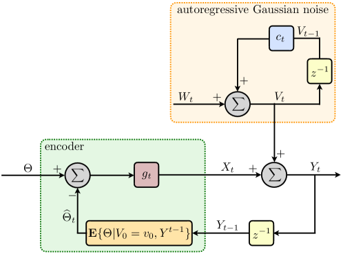
Figure I.1: Mathematical model of the AGN channel driven by a time-varying AR$(c_{t};v_{0}),c_{t}\in(-\infty,\infty),K_{W_{t}}>0\;\forall t$ noise, with Butman’s linear feedback coding scheme. The model in [1] corresponds to the restriction AR$(c;v_{0}),K_{W_{t}}=K_{W}\forall t$. $g_{n},n=1,2,\ldots$ is gain sequence multiplying the estimation error.

Throughout the paper, we use the following notation.
AR$(c_{t};v_{0})$, denotes the time-varying autoregressive unit memory noise $V^{n}$, with $c_{t}\in(-\infty,\infty),K_{W_{t}}\in(0,\infty),t=1,\ldots,n$, AR$(c;v_{o})$ denotes its restriction to time-invariant, with $c_{t}=c\in(-\infty,\infty),K_{W_{t}}=K_{W}\in(0,\infty),t=1,\ldots,n$. The stable AR$(c;v_{0})$ noise corresponds to $c\in(-1,1)$.
A time-varying AR noise without an initial state is denoted by AR$(c_{t}),c_{t}\in(-\infty,\infty)$, and corresponds to the case, the RV $V_{0}$ generates the trivial information, i.e., the sigma$-$algebra generated by $V_{0}$ is $\sigma\{V_{0}\}=\{\emptyset,\Omega\}$.
$I(\Theta;Y^{n}|v_{0})$ denotes the mutual information between the Gaussian message $\Theta$ and the sequence $Y^{n}$ conditioned on $V_{0}=v_{0}$, and $I(\Theta;Y^{n})$ denotes the mutual information between $\Theta$ and the sequence $Y^{n}$.
From the above formulation, follows that, if $V_{0}$ generates the trivial information, then $I(\Theta;Y^{n}|V_{0})=I(\Theta;Y^{n})$; in this case $I(\Theta;Y^{n})$ depends on the distribution of the RV $V_{1}$, i.e., ${\bf P}_{V_{1}}$ and $V_{1}=W_{1}$.

Butman in the 1976 paper [1], considered (I.1)-(I.8), for AR$(c;v_{0}),c\in[-1,1]$, i.e., $c_{t}=c\;\forall t$, $K_{\Theta}=1$, and derived achievable feedback rates, based on the optimization problem

$$C_{n}^{L}(\kappa,v_{0})\stackrel{{\scriptstyle\triangle}}{{=}}\sup_{X_{t}=e_{t}(v_{0},\Theta,Y^{t-1}),\;e_{t}(\cdot)\>\>\mbox{is linear},\>\>t=1,\ldots,n:\>\frac{1}{n}{\bf E}\big{\{}\sum_{t=1}^{n}\big{(}X_{t}\big{)}^{2}\Big{|}V_{0}=v_{0}\big{\}}\leq\kappa}\frac{1}{n}I(\Theta;Y^{n}|v_{0}),$$ (I.9)

and its per unit time limit,

$$C^{L}(\kappa,v_{0})=\lim_{n\longrightarrow\infty}C_{n}^{L}(\kappa,v_{0})$$ (I.10)

provided the supremum and limit exist. In particular, Butman proved that linear strategies $e_{t}(\cdot),t=1,\ldots,n$ are given by [1, eqn(17)],

$$e_{t}(v_{0},\Theta,Y^{t-1})=g_{t}\Big{(}\Theta-{\bf E}\Big{\{}\Theta\Big{|}Y^{t-1},V_{0}=v_{0}\Big{\}}\Big{)},\hskip 14.45377ptt=2,\ldots,n,\hskip 14.45377pte_{1}(v_{0},\Theta)=g_{1}\Theta$$ (I.11)

where $g_{1},g_{2},\ldots,g_{n}$ is a sequence of nonrandom real numbers. Hence, the supremum in (I.9) is replaced by the supremum over the sequence $g_{1},g_{2},\ldots,g_{n}$ that satisfies the average power constraint.

Remark I.1.

The AGN Channel Driven by Noise without Initial State
The variation of the above AGN channel without an initial state, follows directly from the Tienan and Schalkwijk [4] and Butman [1] formulation, by letting $V_{0}$ generate the trivial information, i.e., the sigma$-$algebra generated by $V_{0}$ is $\sigma\{V_{0}\}=\{\emptyset,\Omega\}$. In such a formulation $C_{n}^{L}(\kappa,v_{0}),C_{n}^{L}(\kappa,v_{0})$ are replaced by $C_{n}^{L}(\kappa,{\bf P}_{V_{1}}),C_{n}^{L}(\kappa,{\bf P}_{V_{1}})$, which emphasize their dependence on the distribution ${\bf P}_{V_{1}}$ of $V_{1}$, instead of initial state $V_{0}=v_{0}$.

[1] is focused on the optimization problem (I.9) and its per unit time limit (I.10), with coding scheme (I.11), and in particular on the derivation of upper and lower bounds. It will become apparent (in subsequent sections) that Butman’s lower bound is derived using a per-symbol average power constraint at each transmission time, i.e., ${\bf E}\Big{\{}\big{(}X_{n}\big{)}^{2}\Big{|}V_{0}=v_{0}\Big{\}}\leq\kappa,n=1,2,\ldots$, and not $\frac{1}{n}{\bf E}\big{\{}\sum_{t=1}^{n}\big{(}X_{t}\big{)}^{2}\Big{|}V_{0}=v_{0}\big{\}}\leq\kappa$.
Over the years, the following result, is used extensively in the literature, such as, [15, 16].

1. Butman’s lower bound on $C_{n}^{L}(\kappa,v_{0})$ and $C^{L}(\kappa,v_{0})$, and Butman’s Conjecture, that these bounds correspond to the feedback capacity [1, Abstract].

In particular, [2] proved that Butman’s Conjecture is correct, and the frequency and time-domain characterizations of feedback capacity [2, Theorem 4.1 and Theorem 6.1], reproduce Butman’s lower bound on feedback capacity.

I-B Main Results on the Linear Code of [1]

We prove the following conclusion.

(C)

Butman’s [1, Abstract] calculation of the rate $\lim_{n\longrightarrow\infty}C_{n}^{L}(\kappa,v_{0})$ for the AR$(c;v_{0}),c\in[-\infty,\infty]$ noise, known as Butman’s lower bound and conjecture on feedback capacity, based on coding scheme (I.11), corresponds to an unbounded sequence $g_{1},g_{2},\ldots$, in the sense that, $\lim_{n\longrightarrow\infty}|g_{n}|=+\infty$.

Theorem I.3 presents some of the consequences of (C). To prove (C) we will make use of Theorem I.1 (below), known as the ratio test theorem [17, Theorem 3.34].

Theorem I.1 (The Ratio Test).

Consider any sequence of real numbers $\{a_{n}:n=1,2,\ldots\}$.
(a) Suppose that $\lim_{n\longrightarrow\infty}\left|{a_{n+1}}/{a_{n}}\right|=L$. If $L<1$, then the series $\sum_{n=0}^{\infty}{a_{n}}$ converges absolutely, if $L>1$ the series diverges, and if $L=1$ this test gives no information.
(b) If $\lim_{n\longrightarrow\infty}\left|{a_{n+1}}/{a_{n}}\right|>1$, then $\lim_{n\longrightarrow\infty}|a_{n}|=+\infty$; if $\lim_{n\longrightarrow\infty}\left|{a_{n+1}}/{a_{n}}\right|<1$, then $\lim_{n\longrightarrow\infty}|a_{n}|=0$.

Further, as mentioned earlier, to provide additional insight, we present an alternative derivation of Butman’s lower bound $C_{n}^{L}(\kappa,v_{0})$ for any $n=1,2,\ldots$, as stated in Theorem I.2 (below), which is also valid for the AR$(c_{t};v_{0}),c_{t}\in(-\infty,\infty)$ noise.

Theorem I.2 (Characterizations of $C_{n}^{L}(\kappa,v_{0})$ and $C_{n}^{L}(\kappa,{\bf P}_{V_{1}})$).

Consider the AGN channel defined by (I.1)-(I.8), i.e., with AR$(c_{t};v_{0})$ or AR$(c_{t})$, for any $c_{t}\in(-\infty,\infty),t=0,1,\ldots$.
(a) Total Average Power Constraint. The maximization over all linear coding schemes, (I.11) (without initial state, i.e., for AR$(c_{t})$ noise) of mutual information $I(\Theta;Y^{n})$, subject to total average power, $\frac{1}{n}{\bf E}\big{\{}\sum_{t=1}^{n}\big{(}X_{t}\big{)}^{2}\big{\}}\leq\kappa$, is given by

$$C_{n}^{L}(\kappa,{\bf P}_{V_{1}})\stackrel{{\scriptstyle\triangle}}{{=}}\sup_{g_{t},\>t=1,\ldots,n:\>\>\frac{1}{n}\big{\{}g_{1}^{2}K_{\Theta}+\sum_{t=2}^{n}g_{t}^{2}\Sigma_{t-1}\big{\}}\leq\kappa}\frac{1}{2}\Big{\{}\log\Big{(}\frac{g_{1}^{2}K_{\Theta}+K_{V_{1}}}{K_{V_{1}}}\Big{)}$$

$$\hskip 14.45377pt\hskip 14.45377pt\hskip 14.45377pt\hskip 14.45377pt+\sum_{t=2}^{n}\log\Big{(}\frac{\Big{(}1-c_{t}\frac{g_{t-1}}{g_{t}}\Big{)}^{2}g_{t}^{2}\Sigma_{t-1}+K_{W_{t}}}{K_{W_{t}}}\Big{)}\Big{\}},$$ (I.12)

subject to $$\Sigma_{t},t=1,\ldots,n g_{1},\ldots,g_{n}$$ that satisfies the recursion and controlled by ,

$$\Sigma_{t}=\frac{K_{W_{t}}\Sigma_{t-1}}{\Big{(}g_{t}-c_{t}g_{t-1}\Big{)}^{2}\Sigma_{t-1}+K_{W_{t}}},\hskip 14.45377ptt=2,\ldots,n,$$ (I.13)

$$\Sigma_{1}=\frac{K_{\Theta}K_{V_{1}}}{g_{1}^{2}K_{\Theta}+K_{V_{1}}}.$$ (I.14)

(b) Pointwise Average Power Constraint. The maximization over all linear coding schemes, (I.11) (for AR$(c_{t})$ noise) of mutual information $I(\Theta;Y^{n})$, subject to pointwise average power, ${\bf E}\big{\{}\big{(}X_{t}\big{)}^{2}\big{\}}\leq\kappa_{t},t=1,\ldots,n$, is given by

$$C_{n}^{L}(\kappa_{1},\ldots,\kappa_{n},{\bf P}_{V_{1}})\stackrel{{\scriptstyle\triangle}}{{=}}\sup_{g_{t},\>t=1,\ldots,n:\>\>g_{1}^{2}K_{\Theta}\leq\kappa_{1},\>g_{t}^{2}\Sigma_{t-1}\leq\kappa_{t},\>t=2,\ldots,n}\frac{1}{2}\Big{\{}\log\Big{(}\frac{g_{1}^{2}K_{\Theta}+K_{V_{1}}}{K_{V_{1}}}\Big{)}$$

$$\hskip 14.45377pt\hskip 14.45377pt\hskip 14.45377pt\hskip 14.45377pt\hskip 14.45377pt\hskip 14.45377pt+\sum_{t=2}^{n}\log\Big{(}\frac{\Big{(}1-c_{t}\frac{g_{t-1}}{g_{t}}\Big{)}^{2}g_{t}^{2}\Sigma_{t-1}+K_{W_{t}}}{K_{W_{t}}}\Big{)}\Big{\}},$$ (I.15)

subject to $$\Sigma_{t},t=1,\ldots,n g_{1},\ldots,g_{n}$$ that satisfies recursion (I.13), (I.14) and controlled by . (I.16)

(c) The statements of parts (a) and (b) hold, when the noise is replaced by AR$(c_{t};v_{0})$, with $V_{0}=v_{0}$ the initial state known to the encoder, and with $K_{V_{1}}$ replaced by $K_{W_{1}}$, and $C_{n}^{L}(\kappa,{\bf P}_{V_{1}})=C_{n}^{L}(\kappa,v_{0}),C_{n}^{L}(\kappa_{1},\ldots,\kappa_{n},{\bf P}_{V_{1}})=C_{n}^{L}(\kappa_{1},\ldots,\kappa_{n},v_{0})$.

Proof.

The proof is given in Section II. ∎

In Section I-C, we show that Butman’s lower bound of the AR unit memory noise, corresponds to parameters $K_{W_{t}}=K_{W},c_{t}=c\in[-1,1],t=1,2\ldots$, Gaussian message $\Theta\in G(0,1)$, i.e, $K_{\Theta}=1$, and it is obtained from Theorem I.2.(c), i.e., $C_{n}^{L}(\kappa_{1},\ldots,\kappa_{n},v_{0})$, by invoking Butman’s strategy [1, 4 lines below eqn(19)], $sgn(g_{n})=-sgn(cg_{n-1}),n=2,3$.

I-C Observations on the Lower Bound on Feedback Capacity of [1, 5]

Now, we turn our attention to Butman’s assumptions, formulation, and the main steps of the derivation of the lower bound in [1], to verify our observation and claims. It is noted that Butman’s lower bound is also derived by Wolfowitz [5], by transmitting one of $e^{nR}$ messages and maximizing the operational rate $R$ (i.e., without using information theoretic measures of mutual information etc); rather, by applying the operational definition of achievable rates.

Below, we make an observation which is easy to verify.

Observation I.1.

By evaluating $C_{n}^{L}(\kappa_{1},\ldots,\kappa_{n},v_{0})$, described in Theorem I.2.(c), for the parameters $K_{W_{t}}=K_{W},c_{t}=c\in[-1,1],t=1,2\ldots$, Gaussian message $\Theta\in G(0,1)$, i.e, $K_{\Theta}=1$, at Butman’s strategy [1, 4 lines below eqn(19)],

$$sgn(g_{n})=-sgn(cg_{n-1}),n=2,3,\ \ \mbox{ implies}\ \ \sum_{j=2}^{n}\big{(}g_{j}-cg_{j-1}\big{)}^{2}=\sum_{j=2}^{n}(g_{j})^{2}\Big{(}1+|c||\frac{g_{j-1}}{g_{j}}|\Big{)}^{2},$$ (I.17)

then by simple algebra we obtain Butman’s and Wolfowitz’s lower bound (this is also verified in the sequel).

Fact 1. Butman [1] and also Wolfowitz [5], considered the AGN channel driven by the AR$(c),c\in[-1,1]$ noise, i.e., $W_{t}\in G(0,K_{W})\forall t$, and applied the linear time-varying coding strategy of a Gaussian message $\Theta\in G(0,1)$, i.e., zero mean and unit variance $K_{\Theta}=1$, to obtain

$$X_{n}=g_{n}\Big{(}\Theta-{\bf E}\Big{\{}\Theta\Big{|}Y^{n-1},V_{0}=v_{0}\Big{\}}\Big{)},\hskip 14.45377ptn=2,3,\ldots,\hskip 14.45377ptX_{1}=g_{1}\Theta,$$ (I.18)

$$\frac{1}{n}{\bf E}\Big{\{}\sum_{t=1}^{n}\big{(}X_{t}\big{)}^{2}\Big{|}V_{0}=v_{0}\Big{\}}=\frac{1}{n}\sum_{t=1}^{n}\kappa_{t}\leq\kappa,\hskip 14.45377pt\kappa_{t}\stackrel{{\scriptstyle\triangle}}{{=}}g_{t}^{2}\Sigma_{t-1},\hskip 7.22743ptt=2,\ldots,n,\hskip 7.22743pt\kappa_{1}\stackrel{{\scriptstyle\triangle}}{{=}}g_{1}^{2},$$ (I.19)

$$\Sigma_{t}\stackrel{{\scriptstyle\triangle}}{{=}}{\bf E}\Big{\{}\Big{(}\Theta-{\bf E}\Big{\{}\Theta\Big{|}Y^{t},V_{0}=v_{0}\Big{\}}\Big{)}^{2}\Big{\}}=\frac{K_{W}}{g_{1}^{2}+\sum_{j=2}^{t}\big{(}g_{j}-cg_{j-1}\big{)}^{2}+K_{W}},\hskip 7.22743ptt=2,\ldots,n,$$ (I.20)

$$\Sigma_{1}=\frac{K_{W}}{g_{1}^{2}+K_{W}}$$ (I.21)

Fact 2. [1, 4 lines below eqn(19)], restricted the strategy $g_{n}$ to the one that increases the signal-to-noise ratio, $\frac{g_{1}^{2}+\sum_{j=2}^{t}\big{(}g_{j}-cg_{j-1}\big{)}^{2}}{K_{W}}$, as follows.

$$sgn(g_{n})=-sgn(cg_{n-1}),\hskip 14.45377ptn=2,3,\ldots\hskip 7.22743pt\Longrightarrow\hskip 7.22743pt\sum_{j=2}^{n}\big{(}g_{j}-cg_{j-1}\big{)}^{2}=\sum_{j=2}^{n}(g_{j})^{2}\Big{(}1+|c||\frac{g_{j-1}}{g_{j}}|\Big{)}^{2}.$$ (I.22)

Fact 3. [1, eqn(26)–eqn(28)] evaluated $I(\Theta;Y^{n}|v_{0})$, by applying the linear coding strategy (I.22) as follows.

$$I(\Theta;Y^{n}|v_{0})= \frac{1}{2}\log\Big{\{}1+\frac{\kappa_{1}}{K_{W}}\Big{\}}+\frac{1}{2}\sum_{t=2}^{n}\log\Big{\{}1+\Big{(}g_{t}-cg_{t-1}\Big{)}^{2}\frac{\Sigma_{t-1}}{K_{W}}\Big{\}}$$ (I.23)

$$= \frac{1}{2}\log\Big{\{}1+\frac{\kappa_{1}}{K_{W}}\Big{\}}+\frac{1}{2}\sum_{t=2}^{n}\log\Big{\{}1+\Big{(}1+\frac{|c|}{\chi_{t}}\Big{)}^{2}\frac{\kappa_{t}}{K_{W}}\Big{\}}\hskip 14.45377pt\mbox{by (\ref{butman_cs__a2})}$$ (I.24)

where $\chi_{n}$ is related to $(g_{n},g_{n-1})$ and satisfies the recursion [1, eqn(23)],

$$\chi_{n}\stackrel{{\scriptstyle\triangle}}{{=}}\Big{|}\frac{g_{n}}{g_{n-1}}\Big{|},\hskip 14.45377ptn=3,4,\ldots,\hskip 14.45377pt\chi_{2}=1+\frac{\kappa_{1}}{K_{W}},$$ (I.25)

$$\chi_{n}^{2}=\Big{\{}1+\Big{(}1+\frac{|c|}{\chi_{n-1}}\Big{)}^{2}\frac{\kappa_{n-1}}{K_{W}}\Big{\}}\frac{\kappa_{n}}{\kappa_{n-1}},\hskip 7.22743ptn=3,4,\ldots$$ (I.26)

Fact 4. Butman’s resulting optimization problem, from Fact 3, reduces to

$${\bf(B1):}\hskip 14.45377pt \frac{1}{n}C_{n}^{L,B1}(\kappa,v_{0})\stackrel{{\scriptstyle\triangle}}{{=}}\sup_{g_{1},\ldots,g_{n}}\Big{\{}\frac{1}{2n}\log\Big{\{}1+\frac{\kappa_{1}}{K_{W}}\Big{\}}+\frac{1}{2n}\sum_{t=2}^{n}\log\Big{\{}1+\Big{(}1+\frac{|c|}{\chi_{t}}\Big{)}^{2}\frac{\kappa_{t}}{K_{W}}\Big{\}}\Big{\}}$$ (I.27)

$$\mbox{ subject to}\hskip 7.22743pt\sum_{t=1}^{n}\kappa_{t}\leq\kappa,\hskip 7.22743pt\kappa_{t}\stackrel{{\scriptstyle\triangle}}{{=}}g_{t}^{2}\Sigma_{t-1},\hskip 7.22743ptt=2,\ldots,n,\hskip 7.22743pt\kappa_{1}=g_{1}^{2},$$ (I.28)

$$\chi_{t}$$ satisfies recursion (I.25), (I.26), (I.29)

$$\Sigma_{t}=\frac{K_{W}}{g_{1}^{2}+\sum_{j=2}^{t}(g_{j})^{2}\big{(}1+\frac{|c|}{\chi_{j}}\big{)}^{2}+K_{W}},\hskip 7.22743ptt=2,\ldots,n\hskip 14.45377pt\mbox{by (\ref{butman_cs__a2})},$$ (I.30)

$$\Sigma_{1}=\frac{K_{W}}{g_{1}^{2}+K_{W}}.$$ (I.31)

Notice that in (B1) one is asked to optimize over $\{g_{1},g_{2},\ldots,g_{n}\}$ subject to constraints, or over $\{\kappa_{1},\kappa_{2},\ldots,\kappa_{n}\}$.

Fact 5. [1] did not provide a solution to $C_{n}^{L,B1}(\kappa,v_{0})$; instead the statement of Butman’s conjecture [1, Abstract] on feedback capacity is based on a variation, based on Assumptions I.1 (below).

Assumptions I.1.

[1] Average point-wise power constraints
Butman’s lower bound on feedback capacity and conjecture [1, Abstract], is based on the single-letter average power at the transmitter (easily verified from [1]), given by

$${\bf E}\Big{\{}\big{(}X_{t}\big{)}^{2}\Big{|}V_{0}=v_{0}\Big{\}}=\kappa,\hskip 7.22743ptt=1,2,\ldots,n\hskip 7.22743pt\Longrightarrow\hskip 7.22743pt\kappa_{t}\stackrel{{\scriptstyle\triangle}}{{=}}g_{t}^{2}\Sigma_{t-1}=\kappa,\hskip 7.22743ptt=2,\ldots,n,\hskip 7.22743pt\kappa_{1}\stackrel{{\scriptstyle\triangle}}{{=}}g_{1}^{2}=\kappa$$ (I.32)

where $\Sigma_{t},t=1,\ldots,n$ satisfies (I.30) and (I.31).

In view of Assumptions I.1, Butman’s lower bound [1, see transition from eqn(23) to eqn(23a) or eqn(28) and paragraph above it], is given as follows.

$${\bf(B2):}\hskip 14.45377pt \frac{1}{n}C_{n}^{L,B2}(\kappa,v_{0})=\frac{1}{2n}\log\Big{\{}1+\frac{\kappa}{K_{W}}\Big{\}}+\frac{1}{2n}\sum_{t=2}^{n}\log\Big{\{}1+\Big{(}1+\frac{|c|}{\chi_{t}}\Big{)}^{2}\frac{\kappa}{K_{W}}\Big{\}}$$ (I.33)

$$\chi_{t} \chi_{t}^{2}=1+\Big{(}1+\frac{|c|}{\chi_{n-1}}\Big{)}^{2}\frac{\kappa}{K_{W}},\hskip 7.22743ptt=3,4,\ldots,\chi_{2}=1+\frac{\kappa}{K_{W}}$$ satisfies recursion , (I.34)

$$g_{t}^{2}\Sigma_{t-1}=\kappa,\hskip 7.22743ptt=2,\ldots,n,\hskip 7.22743ptg_{1}^{2}=\kappa,\hskip 7.22743pt\mbox{$\Sigma_{t},t=1,\ldots,n$ satisfies (\ref{butman_cs_2_aa}), (\ref{butman_cs_2_bb}).}$$ (I.35)

Unlike (B1), in (B2) there is no optimization over $\{g_{1},g_{2},\ldots,g_{n}\}$ or $\{\kappa_{1},\kappa_{2},\ldots,\kappa_{n}\}$.

Fact 6. Butman’s lower bound [1, Abstract, with $m=1$ or eqn(4), eqn(5), eqn(11)] Butman [1, eqn(23a) and paragraph above eqn(28)], which is based on Assumptions I.1 and strategy (I.22), is stated as follows.

$${\bf(B):}\hskip 14.45377ptC^{L,B}(\kappa)\stackrel{{\scriptstyle\triangle}}{{=}}\lim_{n\longrightarrow\infty}\frac{1}{n}C_{n}^{L,B2}(\kappa,v_{0})=\frac{1}{2}\log\chi^{2},$$ (I.36)

where

$$\chi=\lim_{n\longrightarrow\infty}\chi_{n}=\lim_{n\longrightarrow\infty}\Big{|}\frac{g_{n}}{g_{n-1}}\Big{|},$$ (I.37)

$$\mbox{$\chi$ is the positive root of}\hskip 7.22743pt\chi^{4}-\chi^{2}-\frac{\kappa}{K_{W}}\Big{(}\chi+|c|\Big{)}^{2}=0,\hskip 14.45377pt|c|\leq 1,\hskip 7.22743ptK_{W}>0,\hskip 7.22743pt\kappa\geq 0,$$ (I.38)

Butman [1] conjectured that $C^{L,B}(\kappa)$ is the feedback capacity.

Remark I.2.

A comparison of $C^{L,B}(\kappa)$ to an upper bound derived by Tienan and Schalkwijk [4, Section I] is discussed in [1, eqn(1) and eqn(2)]. Ozarow [9] and Dembo [8] re-visited Butman’s lower bound and derived upper bounds on feedback rates.

To complete our observations on Butman’s problems we note two more facts.

Fact 7. If we do not impose Butman’s restriction that strategies $g_{n}$ satisfy $sgn(g_{n})=-sgn(cg_{n-1}),n=2,3,\ldots$, i.e., (I.22) is not assumed, then the optimization problem (B1) and statement (B2), are replaced by (P1) and (P2), respectively, given below.

$${\bf(P1):}\hskip 14.45377pt \frac{1}{n}C_{n}^{L,P1}(\kappa,v_{0})\stackrel{{\scriptstyle\triangle}}{{=}}\sup_{g_{1},\ldots,g_{n}}\Big{\{}\frac{1}{2n}\log\Big{\{}1+\frac{\kappa_{1}}{K_{W}}\Big{\}}+\frac{1}{2n}\sum_{t=2}^{n}\log\Big{\{}1+\Big{(}g_{t}-cg_{t-1}\Big{)}^{2}\frac{\Sigma_{t-1}}{K_{W}}\Big{\}}\Big{\}}$$ (I.39)

$$\mbox{ subject to}\hskip 7.22743pt\frac{1}{n}\sum_{t=1}^{n}\kappa_{t}\leq\kappa,\hskip 7.22743pt\kappa_{t}\stackrel{{\scriptstyle\triangle}}{{=}}g_{t}^{2}\Sigma_{t-1},\hskip 7.22743ptt=2,\ldots,n,\hskip 7.22743pt\kappa_{1}=g_{1}^{2},$$ (I.40)

$$\Sigma_{t}=\frac{K_{W}}{g_{1}^{2}+\sum_{j=2}^{t}\big{(}g_{j}-cg_{j-1}\big{)}^{2}+K_{W}},\hskip 7.22743ptt=2,\ldots,n,$$ (I.41)

$$\Sigma_{1}=\frac{K_{W}}{g_{1}^{2}+K_{W}},$$ (I.42)

$${\bf(P2):}\hskip 14.45377pt \frac{1}{n}C_{n}^{L,P2}(\kappa,v_{0})\stackrel{{\scriptstyle\triangle}}{{=}}\sup_{g_{1},\ldots,g_{n}}\Big{\{}\frac{1}{2n}\log\Big{\{}1+\frac{\kappa_{1}}{K_{W}}\Big{\}}+\frac{1}{2n}\sum_{t=2}^{n}\log\Big{\{}1+\Big{(}g_{t}-cg_{t-1}\Big{)}^{2}\frac{\Sigma_{t-1}}{K_{W}}\Big{\}}\Big{\}}$$ (I.43)

$$\mbox{ subject to}\hskip 7.22743ptg_{t}^{2}\Sigma_{t-1}=\kappa,\hskip 7.22743ptt=2,\ldots,n,\hskip 7.22743ptg_{1}^{2}=\kappa,$$ (I.44)

$$\Sigma_{t},t=1,\ldots,n\hskip 7.22743pt\mbox{satisfies (\ref{butman_cs_2_aap}), (\ref{butman_cs_2_bbp}).}$$ (I.45)

Notice (P1), (P2) are optimization problems, where $\{g_{1},g_{2},\ldots,g_{n}\}$ control $\{\Sigma_{1},\Sigma_{2},\ldots,\Sigma_{n}\}$.
In Section I-D we compare the numerical solutions of (B2) and (B) to (P2).

The next theorem, is an application of the ratio test theorem to Butman’s lower bound $C^{L,B}(\kappa)$ given by (I.36)-(I.37).

Theorem I.3.

On Butman’s lower bound
Consider the lower bound [1], $C^{L,B}(\kappa)=\frac{1}{2}\log\chi^{2}$ given by (I.36)-(I.38).
If $\lim_{n\longrightarrow\infty}\left|{g_{n}}/{g_{n-1}}\right|=\chi>1$, then $\lim_{n\longrightarrow\infty}|g_{n}|=+\infty$.
If $\lim_{n\longrightarrow\infty}\left|{g_{n}}/{g_{n-1}}\right|=\chi<1$, then $\lim_{n\longrightarrow\infty}|g_{n}|=0$, and $C^{L,B}(\kappa)=\frac{1}{2}\log\max\{1,\chi^{2}\}=0\;\forall\kappa\in[0,\infty)$.

Proof.

Suppose Butman’s sequence $\{g_{1},g_{2},\ldots,g_{n}\}$, corresponding to (I.37), (I.38), i.e., computed using $\chi=\lim_{n\longrightarrow\infty}\chi_{n}=\lim_{n\longrightarrow\infty}\Big{|}\frac{g_{n}}{g_{n-1}}\Big{|}$, such that $\chi$ is is the real positive root of the quadric equation (I.38), with $|\chi|>1$. Then by Theorem I.1.(b), sequence $\{g_{1},g_{2},\ldots,g_{n}\}$, is such that, $|g_{n}|\longrightarrow\infty$, as $n\longrightarrow\infty$. On the other hand, Theorem I.1.(b), if $|\chi|<1$ then $|g_{n}|\longrightarrow 0$, as $n\longrightarrow\infty$, and since $C^{L,B}(\kappa)$ is computed using mutual information which takes values in $[0,\infty]$ then the claim holds. ∎

This implies, Butman ’s lower bound is achieved by an unbounded sequence of coding gains $|g_{1}|,|g_{2}|,\ldots$. Therefore, such coding schemes are not practical, and moreover they are fragile, at least for transmission intervals $\{1,2,\ldots,n\}$ of moderate duration $n$. By fragile, we mean, any mismatch of the estimation error $\Theta-{\bf E}\Big{\{}\Theta\Big{|}Y^{n-1},V_{0}=v_{0}\Big{\}}$ due to any additional external noise in the Gaussian channel not accounted for, at any given time of transmission, will be amplified by the scaling $g_{n}$ (see abstract).

Further to the above, it should be apparent that optimization problem $(\mathbf{B1})$, which uses a total average power constraint, i.e., (I.27)-(I.29), is also achieved by an unbounded sequence $|g_{1}|,|g_{2}|,\ldots$.

Remark I.3.

From the above follows that convergence of the sequence $\chi_{n},n=1,2,\ldots$ does not imply convergence of the sequence $|g_{n}|,n=1,2,\ldots$. In fact, if $|g_{n}|,n=1,2,\ldots$ converges to $|g|$ then necessarily $\chi_{n},n=1,2,\ldots$ convergences to $\chi=1$, and the value of the lower bound, is $\frac{1}{2}\log\chi^{2}=0$.

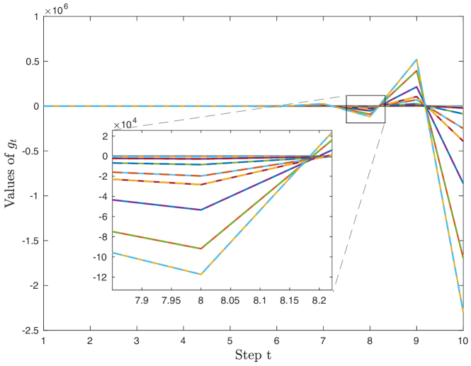
Figure I.2: Numerical example with which it is shown that Butman’s strategy $g_{t},t=1,2,\ldots$ , shown in solid line, as well as the numerical evaluation of (P2), shown in dashed line, for $n=10$ have values of $g_{t},t=1,\ldots,n$ that are similar and grow unbounded. The small differences, however, lead to the gap in the solution, as shown in Fig. I.3, further supporting our claim about the fragility of Butman’s strategy $g_{1},g_{2},\ldots$. For the simulations, we used $K_{\Theta}=K_{W}=K_{V}=1$, $c=0.5$. The values of the sequence $|g_{1}|,|g_{2}|,\ldots,|g_{n}|$ grows unbounded, as predicted by Theorem I.3.

I-D Simulations of Butman’s Coding Scheme

Figure I.3 is a comparison between the numerical evaluation of (B2), (B) and (P2). Notice that (B2) and (B) are derived by using Butman’s strategy (I.22). For (B2), once $\chi_{t},t=1,2,\ldots,n$ is computed then $g_{t}^{2}\Sigma_{t-1}=\kappa,t=2,\ldots,n,g_{1}^{2}=\kappa,$ and $g_{t},t=1,\ldots,n$ is found from $\Sigma_{t},t=1,\ldots,n$ that satisfies (I.30), (I.31)

While the values of the sequence $g_{1},g_{2},\ldots,g_{n}$ are similar, and their absolute values grow unbounded, as it is shown in Fig. I.2, the numerical evaluation of optimization problem (P2) for $n=10$ performs better than Butman’s lower bound (B2) (which is based on Butman’s strategy (I.22)), even for $n=20$. Therefore, for finite $n$, simulations show that Butman’s strategy (I.22) leading to (B2), is not optimal. Note that for values of $n>10$, the numerical optimization problem (P2) is difficult to complete, because the sequence $|g_{n}|$ grows unbounded, and the numerical optimization does not converge for the maximum number of iterations considered. Similarly, it is difficult to determine $g_{t},t=1,2,\ldots,n$ of (B2) for large $n$. Nevertheless, the main point that Butman’s strategy (I.22) is not optimal for finite $n$, can be inferred from the simulations of (P2) for $n=10$.

Figure I.3: Numerical comparisons of rates based on (B2), (P2) and asymptotic limit, called Batman’s lower bound based on (B). Problem (P2) is solved using standard MATLAB optimization functions (for $n=10$). For the simulations, we used $K_{\Theta}=K_{W}=K_{V}=1$, $c=0.5$. The asymptotic for Butman’s strategy seems to be optimal as $n\to\infty$, but it is not optimal for a finite $n$.

On the other hand, the calculation of asymptotic limit based on (B), gives a value which is higher than (B2) calculated for $n=10$ and $n=20$. This is expected, because the rate based on (B2), i.e., $\frac{1}{n}C_{n}^{L,B2}(\kappa,v_{0})$, is nondecreasing with $n$. On other hand, the rate based on (P2), i.e., $\frac{1}{n}C_{n}^{L,P2}(\kappa,v_{0})$, is also nondecreasing with $n$, but it was not possible to compute it for large values of $n$, because i) $|g_{1}|,|g_{2}|,\ldots$ grows unbounded, and it is difficult to compute it numerically, even for moderate values of $n$ beyond $10$, and ii) an analytic expression of (P2) is not available.

Observation I.2.

On Butman’s strategy (I.22)
Simulations show that Butman’s strategy $sgn(g_{n})=-sgn(cg_{n-1})$, $n=2,3,\ldots$, i.e., which is used to obtain the recursion $\chi_{n},n=1,2,\ldots$ is not optimal for finite $n$, since the numerical optimization problem (P2) produces another sequence $g_{n}$ with higher value of rate (see Fig. I.3). These simulations highlight the severe limitations of Butman’s scheme, since it is sub-optimal for small number of transmissions $n$, and highly impractical for large number of transmissions $n$, because $|g_{1}|,|g_{2}|,\ldots$ grows unbounded.

II Independent Derivation of Butman’s Lower Bound and Additional Discussion

In this section we provide the derivation of Theorem I.2, and then we show how to recover, as degenerate cases, Butman’s lower bounds.

We consider the AGN channel defined by (I.1)- (I.8), without an initial state, and we derive the characterization of $C_{n}^{L}(\kappa,{\bf P}_{V_{1}})$, with coding scheme defined by (I.9) and (I.11), respectively, (without an initial state). The analysis below, shows that, Butman’s equations can be obtained for any time-varying noise with $c_{t}\in(-\infty,\infty)$.

Theorem II.1.

Preliminary characterization of $C_{n}^{L}(\kappa,{\bf P}_{V_{1}})$
Consider the AGN, driven by a time-varying AR$(c_{t}),t\in(-\infty,\infty)$ noise, without initial state.
Define the conditional mean and error covariance by

$$\widehat{\Theta}_{t}\stackrel{{\scriptstyle\triangle}}{{=}} {\bf E}\Big{\{}\Theta\Big{|}Y^{t}\Big{\}},\hskip 14.45377pt\Sigma_{t}\stackrel{{\scriptstyle\triangle}}{{=}}{\bf E}\Big{\{}\Big{(}\Theta-\widehat{\Theta}_{t}\Big{)}^{2}\Big{|}Y^{t}\Big{\}},\hskip 7.22743ptt=1,\ldots,n.$$ (II.46)

Consider the linear coding scheme

$$X_{t}= g_{t}\Big{(}\Theta-\widehat{\Theta}_{t-1}\Big{)},\hskip 7.22743ptt=2,\ldots,n,\hskip 7.22743ptX_{1}=g_{1}\Theta,$$ (II.47)

$$Y_{t}= g_{t}\Big{(}\Theta-\widehat{\Theta}_{t-1}\Big{)}+V_{t},\hskip 7.22743ptt=2,\ldots,n,$$ (II.48)

$$= g_{t}\Big{(}\Theta-\widehat{\Theta}_{t-1}\Big{)}-c_{t}g_{t-1}\Big{(}\Theta-\widehat{\Theta}_{t-2}\Big{)}+cY_{t-1}+W_{t}\hskip 14.45377pt\mbox{by $V_{t-1}=Y_{t-1}-X_{t-1}$}$$ (II.49)

$$Y_{1}= g_{1}\Theta+V_{1},$$ (II.50)

$${\bf E} \big{\{}\sum_{t=1}^{n}\big{(}X_{t}\big{)}^{2}\big{\}}=\frac{1}{n}\sum_{t=1}^{n}\kappa_{t}\leq\kappa,\hskip 14.45377pt\kappa_{t}=g_{t}^{2}\Sigma_{t-1},\hskip 7.22743ptt=2,\ldots,n,\hskip 14.45377pt\kappa_{1}=g_{1}^{2}K_{\Theta}.$$ (II.51)

Then the following hold.
(a) The innovations process of $Y^{n}$ denoted by $I^{n}$ is an orthogonal Gaussian process, $I_{t}\in G(0,K_{I_{t}}),t=1,\ldots$, given by

$$I_{t}\stackrel{{\scriptstyle\triangle}}{{=}} Y_{t}-{\bf E}\Big{\{}Y_{t}\Big{|}Y^{t-1}\Big{\}},\hskip 14.45377ptt=2,\ldots,n$$ (II.52)

$$= \Big{(}g_{t}-c_{t}g_{t-1}\Big{)}\Big{(}\Theta-\widehat{\Theta}_{t-1}\Big{)}+W_{t},$$ (II.53)

$$I_{1}= g_{1}\Theta+V_{1}.$$ (II.54)

where

$$K_{I_{t}}\stackrel{{\scriptstyle\triangle}}{{=}} {\bf E}\Big{\{}\big{(}I_{t}\Big{)}^{2}\Big{\}}=\Big{(}g_{t}-c_{t}g_{t-1}\Big{)}^{2}{\bf E}\Big{\{}\Big{(}\Theta-\widehat{\Theta}_{t-1}\big{\}}\Big{)}^{2}\Big{\}}+K_{W_{t}},\hskip 14.45377ptt=2,3,\ldots,$$ (II.55)

$$= \Big{(}g_{t}-c_{t}g_{t-1}\Big{)}^{2}\Sigma_{t-1}+K_{W_{t}}$$ (II.56)

$$K_{I_{1}}\stackrel{{\scriptstyle\triangle}}{{=}} {\bf E}\Big{\{}\big{(}I_{1}\Big{)}^{2}\Big{\}}=g_{1}^{2}K_{\Theta}+K_{V_{1}}$$ (II.57)

and where the mean-square error $\Sigma_{t}$ and estimate $\widehat{\Theta}_{t}$ satisfy the recursions

$$\Sigma_{t}=\frac{K_{W_{t}}\Sigma_{t-1}}{\Big{(}g_{t}-c_{t}g_{t-1}\Big{)}^{2}\Sigma_{t-1}+K_{W_{t}}},\hskip 14.45377ptt=2,\ldots,n,$$ (II.58)

$$\Sigma_{1}=\frac{K_{\Theta}K_{V_{1}}}{g_{1}^{2}K_{\Theta}+K_{V_{1}}},$$ (II.59)

$$\widehat{\Theta}_{t}=\widehat{\Theta}_{t-1}+\frac{\Big{(}g_{t}-c_{t}g_{t-1}\Big{)}\Sigma_{t-1}}{\Big{(}g_{t}-c_{t}g_{t-1}\Big{)}^{2}\Sigma_{t-1}+K_{W_{t}}}I_{t},\hskip 14.45377ptt=2,\ldots,n,$$ (II.60)

$$\widehat{\Theta}_{1}=\frac{g_{1}K_{\Theta}}{g_{1}^{2}K_{\Theta}+K_{V_{1}}}I_{1}.$$ (II.61)

The mutual information between the Gaussian RV $\Theta$ and $Y^{n}$, is given by

$$I(\Theta;Y^{n})= H(Y^{n})-H(V^{n})$$ (II.62)

$$= \sum_{t=1}^{n}H(I_{t})-H(V_{1})-\sum_{t=2}^{n}H(W_{t})$$ (II.63)

$$= \frac{1}{2}\log\Big{(}\frac{g_{1}^{2}K_{\Theta}+K_{V_{1}}}{K_{V_{1}}}\Big{)}+\frac{1}{2}\sum_{t=2}^{n}\log\Big{(}\frac{\Big{(}g_{t}-c_{t}g_{t-1}\Big{)}^{2}\Sigma_{t-1}+K_{W_{t}}}{K_{W_{t}}}\Big{)}$$ (II.64)

$$= \frac{1}{2}\log\Big{(}\frac{\kappa_{1}+K_{V_{1}}}{K_{V_{1}}}\Big{)}+\frac{1}{2}\sum_{t=2}^{n}\log\Big{(}\frac{\Big{(}1-c_{t}\frac{g_{t-1}}{g_{t}}\Big{)}^{2}\kappa_{t}+K_{W_{t}}}{K_{W_{t}}}\Big{)}.$$ (II.65)

(b) Suppose $K_{W_{t}}=K_{W},t=2,\ldots,n$. Then

$$\Sigma_{t}= \frac{K_{W}K_{\Theta}K_{V_{1}}}{g_{1}^{2}K_{W}K_{\Theta}+\sum_{j=2}^{t}\big{(}g_{j}-c_{j}g_{j-1}\big{)}^{2}K_{\Theta}K_{V_{1}}+K_{W}K_{V_{1}}},\hskip 7.22743ptt=2,\ldots,n,$$ (II.66)

$$\Sigma_{1}= \frac{K_{\Theta}K_{V_{1}}}{g_{1}^{2}K_{\Theta}+K_{V_{1}}},$$ (II.67)

$${\bf E}\Big{\{} \sum_{t=1}^{n}\big{(}X_{t}\big{)}^{2}\Big{\}}=\frac{1}{n}\sum_{t=1}^{n}\kappa_{t}\leq\kappa,$$ (II.68)

$$\kappa_{t}= \frac{g_{t}^{2}K_{W}K_{\Theta}K_{V_{1}}}{g_{1}^{2}K_{W}K_{\Theta}+\sum_{j=2}^{t-1}\Big{(}g_{j}-c_{j}g_{j-1}\Big{)}^{2}K_{\Theta}K_{V_{1}}+K_{W}K_{V_{1}}},\hskip 7.22743ptt=2,\ldots,n,$$ (II.69)

$$\kappa_{1}= \frac{g_{1}^{2}K_{\Theta}K_{V_{1}}}{g_{1}^{2}K_{\Theta}+K_{V_{1}}}$$ (II.70)

$$I(\Theta;Y^{n})= \frac{1}{2}\log\Big{(}\frac{g_{1}^{2}K_{\Theta}+K_{V_{1}}}{K_{V_{1}}}\Big{)}+\frac{1}{2}\sum_{t=2}^{n}\log\Big{(}\big{(}1-c_{t}\frac{g_{t-1}}{g_{t}}\big{)}^{2}\frac{\kappa_{t}}{K_{W}K_{\Theta}K_{V_{1}}}+1\Big{)}$$ (II.71)

$$= \frac{1}{2}\log\Big{(}\frac{g_{1}^{2}K_{\Theta}+K_{V_{1}}}{K_{V_{1}}}\Big{)}+\frac{1}{2}\sum_{t=2}^{n}\log\Big{(}\chi_{t+1}\frac{\kappa_{t}}{\kappa_{t+1}}\Big{)}$$ (II.72)

where $\chi_{t}\stackrel{{\scriptstyle\triangle}}{{=}}\frac{g_{t}}{g_{t-1}}$, and

$$\chi_{t+1}=\Big{\{}1+\Big{(}1-c_{t}\frac{1}{\chi_{t}}\Big{)}^{2}\frac{\kappa_{t}}{K_{W_{t}}K_{\Theta}K_{V_{1}}}\Big{\}}\frac{\kappa_{t+1}}{\kappa_{t}},\hskip 7.22743ptt=2,\ldots,n,\hskip 7.22743pt\chi_{2}=\frac{g_{2}}{g_{1}}.$$ (II.73)

Proof.

(a) By

$${\bf E}\Big{\{}Y_{t}\Big{|}Y^{t-1}\Big{\}}= -c_{t}g_{t-1}\widehat{\Theta}_{t-1}+c_{t}g_{t-1}{\bf E}\Big{\{}\widehat{\Theta}_{t-2}\Big{|}Y^{t-1}\Big{\}}+c_{t}Y_{t-1}$$ (II.74)

$$= -c_{t}g_{t-1}\widehat{\Theta}_{t-1}+c_{t}g_{t-1}\widehat{\Theta}_{t-2}+c_{t}Y_{t-1}$$ (II.75)

and substituting into $I_{t}$ we obtain (II.52), (II.54). Then (II.55), (II.57) are directly obtained from the independence of $\Theta$ and $W_{t},t=2,\ldots,n,V_{1}$. By mean-square estimation theory, the conditional covariance of $\Theta$ given $Y^{t}$, denoted by $cov(\Theta,\Theta\Big{|}Y^{t})$ is,

$$cov(\Theta,\Theta\Big{|}Y^{t})= cov(\Theta,\Theta\Big{|}Y^{t-1})-\Big{(}cov(\Theta,Y_{t}\Big{|}Y^{t-1})\Big{)}^{2}\Big{(}cov(Y_{t},Y_{t}\Big{|}Y^{t-1})\Big{)}^{-1}$$ (II.76)

$$= cov(\Theta,\Theta\Big{|}Y^{t-1})-\frac{\Big{(}g_{t}-c_{t}g_{t-1}\Big{)}^{2}\Big{(}cov(\Theta,\Theta\Big{|}Y^{t-1})\Big{)}^{2}}{\Big{(}g_{t}-c_{t}g_{t-1}\Big{)}^{2}\Big{(}cov(\Theta,\Theta\Big{|}Y^{t-1})\Big{)}+K_{W_{t}}},\hskip 7.22743ptt=2,\ldots,n,$$ (II.77)

$$cov(\Theta,\Theta\Big{|}Y_{1})= \frac{K_{\Theta}K_{V_{1}}}{g_{1}^{2}K_{\Theta}+K_{V_{1}}}.$$ (II.78)

From the above follows, $cov(\Theta,\Theta\Big{|}Y^{t})={\bf E}\Big{\{}\Big{(}\Theta-\widehat{\Theta}_{t}\Big{)}^{2}\Big{\}}=\Sigma_{t}$. Hence, (II.78), reduces to

$$\Sigma_{t}= \Sigma_{t-1}-\frac{\Big{(}g_{t}-c_{t}g_{t-1}\Big{)}^{2}\Sigma_{t-1}^{2}}{\Big{(}g_{t}-c_{t}g_{t-1}\Big{)}^{2}\Sigma_{t-1}+K_{W_{t}}},\hskip 7.22743ptt=2,\ldots,n,$$ (II.79)

$$\Sigma_{1}= \frac{K_{\Theta}K_{V_{1}}}{g_{1}^{2}K_{\Theta}+K_{V_{1}}}.$$ (II.80)

From (II.79), (II.80) then follows (II.58), (II.59). The conditional mean of of $\Theta$ given $Y^{t}$ is,

$${\bf E}\Big{\{}\Theta\Big{|}Y^{t}\Big{\}}={\bf E}\Big{\{}\Theta\Big{|}Y^{t-1}\Big{\}}+\Big{(}cov(\Theta,Y_{t}\Big{|}Y^{t-1})\Big{)}\Big{(}cov(Y_{t},Y_{t}\Big{|}Y^{t-1})\Big{)}^{-1}\Big{(}Y_{t}-{\bf E}\Big{\{}Y_{t}\Big{|}Y^{t-1}\Big{\}}\Big{)},\hskip 7.22743ptt=2,\ldots,n,$$ (II.81)

$${\bf E}\Big{\{}\Theta\Big{|}Y_{t}\Big{\}}={\bf E}\Big{\{}\Theta\Big{\}}+cov(\Theta,Y_{1})\Big{(}cov(Y_{1},Y_{1})\Big{)}^{-1}\Big{(}Y_{1}-{\bf E}\Big{\{}Y_{1}\Big{\}}\Big{)}.$$ (II.82)

From (II.81), (II.82) and the conditional variance above, then follows (II.60), (II.61). From the above then follows (II.62)-(II.65). (b) Using the assumptions we deduce (II.66)-(II.71). To show (II.72), (II.73) we follow Butman [3]. Let

$$SNR_{t}= g_{1}^{2}K_{W}K_{\Theta}+\sum_{j=2}^{t}\Big{(}g_{j}-c_{t}g_{j-1}\Big{)}^{2}K_{\Theta}K_{V_{1}},\hskip 7.22743ptt=1,2,\ldots,n$$ (II.83)

$$= SNR_{t-1}+g_{t}^{2}\Big{(}1-c\frac{g_{t-1}}{g_{t}}\Big{)}^{2}K_{\Theta}K_{V_{1}}.$$ (II.84)

Hence,

$$SNR_{t}+K_{W}K_{V_{1}}= SNR_{t-1}+g_{t}^{2}\Big{(}1-c_{t}\frac{g_{t-1}}{g_{t}}\Big{)}^{2}K_{\Theta}K_{V_{1}}+K_{W}K_{V_{1}}$$ (II.85)

$$= \Big{(}SNR_{t-1}+K_{W}K_{V_{1}}\Big{)}\Big{(}1+\frac{g_{t}^{2}}{K_{W}K_{V_{1}}+SNR_{t-1}}\big{(}1-c_{t}\frac{g_{t-1}}{g_{t}}\big{)}^{2}\Big{)}$$ (II.86)

$$= \Big{(}SNR_{t-1}+K_{W}K_{V_{1}}\Big{)}\Big{(}1+\frac{\kappa_{t}}{K_{W}K_{\Theta}K_{V_{1}}}\big{(}1-c_{t}\frac{g_{t-1}}{g_{t}}\big{)}^{2}\Big{)}.$$ (II.87)

Letting $\chi_{t}=\frac{g_{t}}{g_{t-1}}$, then

$$1+\frac{\kappa_{t}}{K_{W}K_{\Theta}K_{V_{1}}}\Big{(}1-c_{t}\frac{g_{t-1}}{g_{t}}\Big{)}^{2}=\frac{K_{W}K_{V_{1}}+SNR_{t}}{K_{W}K_{V_{1}}+SNR_{t-1}}=\frac{\kappa_{t}}{\kappa_{t+1}}\chi_{t+1}.$$ (II.88)

From the above follows (II.72), (II.73). ∎

From Theorem II.1 follows an analogous preliminary characterization, for the AR$(c_{t};v_{0}),t\in(-\infty,\infty)$ noise, i.e., when $V_{0}=v_{0}$ is the initial state known to the encoder, as stated in the next corollary.

Corollary II.1.

Preliminary characterization of $C_{n}^{L}(\kappa,v_{0})$
Consider the statement of Theorem II.1, with the AGN channel driven by a time-varying AR$(c_{t};v_{o})$ noise.
Define the conditional mean and error covariance for fixed $V_{0}=v_{0}$, by

$$\widehat{\Theta}_{t}\stackrel{{\scriptstyle\triangle}}{{=}} {\bf E}\Big{\{}\Theta\Big{|}Y^{t},V_{0}=v_{0}\Big{\}},\hskip 14.45377pt\Sigma_{t}\stackrel{{\scriptstyle\triangle}}{{=}}{\bf E}\Big{\{}\Big{(}\Theta-\widehat{\Theta}_{t}\Big{)}^{2}\Big{|}Y^{t},V_{0}=v_{0}\Big{\}},\hskip 7.22743ptt=1,\ldots,n.$$ (II.89)

Consider the linear coding scheme

$$X_{t}= g_{t}\Big{(}\Theta-\widehat{\Theta}_{t-1}\Big{)},\hskip 7.22743ptt=2,\ldots,n,\hskip 7.22743ptX_{1}=g_{1}\Theta,$$ (II.90)

$$Y_{t}= g_{t}\Big{(}\Theta-\widehat{\Theta}_{t-1}\Big{)}+c_{t}V_{t-1}+W_{t},\hskip 7.22743ptt=2,\ldots,n,$$ (II.91)

$$= g_{t}\Big{(}\Theta-\widehat{\Theta}_{t-1}\Big{)}-c_{t}g_{t-1}\Big{(}\Theta-\widehat{\Theta}_{t-2}\Big{)}+c_{t}Y_{t-1}+W_{t}\hskip 14.45377pt\mbox{by $V_{t-1}=Y_{t-1}-X_{t-1}$}$$ (II.92)

$$Y_{1}= g_{1}\Theta+c_{0}V_{0}+W_{1},$$ (II.93)

$${\bf E} \big{\{}\sum_{t=1}^{n}\big{(}X_{t}\big{)}^{2}\Big{|}V_{0}=v_{0}\big{\}}=\frac{1}{n}\sum_{t=1}^{n}\kappa_{t}\leq\kappa,\hskip 14.45377pt\kappa_{t}=g_{t}^{2}\Sigma_{t-1},\hskip 7.22743ptt=2,\ldots,n,\hskip 14.45377pt\kappa_{1}=g_{1}^{2}K_{\Theta}.$$ (II.94)

Then the statements of Theorem II.1.(a), (b) hold, with the following changes: all conditional expectations are replaced by conditional expectations for a fixed $V_{0}=v_{0}$, $I(\Theta;Y^{n})$ is replaced by $I(\Theta;Y^{n}|v_{0})=H(Y^{n}|v_{0})-H(V^{n}|v_{0})$, and $\Sigma_{1}$ is replaced by $\Sigma_{1}=\frac{K_{\Theta}K_{W_{1}}}{g_{1}^{2}K_{\Theta}+K_{W_{1}}}$.

Proof.

This follows by repeating the derivation of Theorem II.1. ∎

From Theorem II.1 follows the validity of Theorem I.2.

Proposition II.1.

Theorem I.2 is correct.

Proof.

(a) By Theorem II.1.(a) follows directly that optimization problem $C_{n}^{L}(\kappa,{\bf P}_{V_{1}})$ is as stated.
(b) This also follows from Theorem II.1.(a), by replacing the total average power constraint by the pointwise average power constraint.
(c) This follows from Corollary II.1, as in parts (a), (b). ∎

By Theorem II.1, follows that $I(\Theta;Y^{n})$ is maximized by the choice of the sequence $g_{1},g_{2},\ldots,g_{n}$ that controls the mean-square error $\Sigma_{t},t=1,\ldots,n$, and satisfies the average power constraint. In general, this is a dynamic optimization problem, with state variable the sequence $\Sigma_{t},t=1,\ldots,n$.

From Theorem II.1, we recover Wolfowitz’s [5] and Butman’s [1] lower bound, and more importantly the assumptions based on which the lower bound is derived.

Proposition II.2.

Reduction of Theorem II.1.(c) to Butman’s lower bound
(a) The statements of Theorem II.1.(c), with $K_{\Theta}=1,K_{V_{1}}=K_{W},c\in[-1,1]$, and strategy $g_{n}$ that satisfies, (I.22), i.e., $sgn(g_{n})=-sgn(cg_{n-1}),n=2,3,\ldots$, reduce to analogous statements derived by Butman [1], i.e., (I.25)-(I.26).
(a) If in addition to (a), i.e., $sgn(g_{n})=-sgn(cg_{n-1}),n=2,3,\ldots$, the average power contraint is replaced by ${\bf E}\Big{\{}\big{(}X_{t}\big{)}^{2}\Big{\}}=\kappa$, $t=1,2,\ldots,n$ (as in Butman [1]) then problem (I.33)-(I.34) is obtained.

Proof.

This is easily verified. ∎

References

- [1] S. Butman, “Linear feedback rate bounds for regressive channels,” IEEE Transactions on Information Theory, vol. 22, no. 3, pp. 363–366, 1976.
- [2] Y.-H. Kim, “Feedback capacity of stationary Gaussian channels,” IEEE Transactions on Information Theory, vol. 56, no. 1, pp. 57–85, 2010.
- [3] S. Butman, “A general formulation of linear feedback communications systems with solutions,” IEEE Transactions on Information Theory, vol. 15, no. 3, pp. 392–400, 1969.
- [4] J. Tienan and J. P. M. Schalkwijk, “An upper bound to the capacity of bandlimited Gaussian autoregressive channel with noiseless feedback,” IEEE Transactions on Information Theory, vol. IT-14, pp. 311–316, May 1974.
- [5] J. Wolfowitz, “Signalling over a gaussian channel with feedback and autoregressive noise,” Journal of Applied Probability, vol. 12, no. 4, pp. 713–723, 1975.
- [6] P. Elias, “Channel capacity without coding,” MIT Research Laboratory of Electronics, Quarterly Report, October 1961, also in Lectures on Communication System Theory, E. Baghdady, Ed., New York: McGraw Hill, 1961.
- [7] J. P. M. Schalkwijk and T. Kailath, “A coding scheme for additive noise channels with feedback-I: no bandwidth constraints,” IEEE Transactions on Information Theory, vol. 12, no. 2, pp. 172–182, April 1966.
- [8] A. Dembo, “On gaussian feedback capacity,” IEEE Transactions on Information Theory, vol. 35, no. 5, pp. 1072–1076, Sept. 1989.
- [9] L. Ozarow, “Upper bounds on the capacity of Gaussian channel with feedback,” IEEE Transactions on Information Theory, vol. 36, no. 1, pp. 156–161, January 1984.
- [10] O. Shayevitz and M. Feder, “Communication with feedback via posterior matching,” in IEEE International Symposium on Information Theory (ISIT), June 24-29 2007, pp. 391–395.
- [11] ——, “The posterior matching feedback scheme: Capacity achieving and error analysis,” in IEEE International Symposium on Information Theory (ISIT), July 6-11 2008, pp. 900–904.
- [12] ——, “Achieving the empirical capacity using feedback: Memoryless additive models,” IEEE Transactions on Information Theory, vol. 55, no. 3, pp. 1269–1295, March 2009.
- [13] S. Yang, A. Kavcic, and S. Tatikonda, “On feedback capacity of power-constrained Gaussian noise channels with memory,” Information Theory, IEEE Transactions on, vol. 53, no. 3, pp. 929–954, March 2007.
- [14] T. Cover and S. Pombra, “Gaussian feedback capacity,” IEEE Transactions on Information Theory, vol. 35, no. 1, pp. 37–43, Jan. 1989.
- [15] T. Liu and G. Han, “Feedback capacity of stationary Gaussian channels further examined,” IEEE Transactions on Information Theory, vol. 64, no. 4, pp. 2494–2506, April 2019.
- [16] C. Li and N. Elia, “Youla coding and computation of gaussian feedback capacity,” IEEE Transactions on Information Theory, vol. 64, no. 4, pp. 3197–3215, April 2019.
- [17] W. Rudin, Principles of mathematical analysis, 3rd ed. McGraw-Hill, 1976.