Universality of nodal count distribution in large metric graphs

Abstract.

An eigenfunction of the Laplacian on a metric (quantum) graph has an excess number of zeros due to the graph’s non-trivial topology. This number, called the nodal surplus, is an integer between 0 and the graph’s first Betti number $\beta$. We study the distribution of the nodal surplus values in the countably infinite set of the graph’s eigenfunctions. We conjecture that this distribution converges to Gaussian for any sequence of graphs of growing $\beta$. We prove this conjecture for several special graph sequences and test it numerically for a variety of well-known graph families. Accurate computation of the distribution is made possible by a formula expressing the nodal surplus distribution as an integral over a high-dimensional torus.

1. Introduction

Denoting by $\nu_{n}$ the number of nodal domains of the $n$-th Laplacian eigenfunction, Courant’s theorem [26, 27] establishes the bound $\nu_{n}\leq n$. Here a “nodal domain” is a maximal connected component of the underlying physical space where the eigenfunction does not vanish. The theorem, originally stated for planar domains, is extremely robust and remains valid for Laplacians on manifolds, with or without boundary, as well as in numerous other settings, see [37] and references therein. It is also valid on discrete and metric graphs [29, 33].

Pleijel [49] strengthened this bound for Dirichlet Laplacians, proving that the ratio $\nu_{n}/n$ is asymptotically bounded away from 1. More recently, it was suggested [21] that the distribution of this ratio carries important domain-specific information. Bogomolny and Schmit [22] made an appealing quantitative conjecture about the mean and variance of $\nu_{n}/n$ based on an analogy with percolation. Remarkably, extensive numerical calculations [12, 39, 44] revealed statistically significant deviations from the Bogomolny-Schmit prediction but only of relative size of less than $5\%$. Mathematical progress is being made within the Random Wave Model, proving that the mean of $\nu_{n}/n$ is non-zero [13, 45, 46] and providing bounds on the variance [47].

In this paper, we focus on the setting of metric graphs. Here, one can equivalently study the number of zeros of the $n$-th eigenfunction, which we denote by $\phi_{n}$. Assuming the eigefunction does not vanish on vertices (which happens generically [18]) and for large enough $n$, the two quantities are directly related by

$$\nu_{n}=\phi_{n}-\beta+1,$$ (1.1)

where $\beta$ is the number of cycles in the graph (the first Betti number). Due to the bounds

$$n-\beta\leq\nu_{n}\leq n,\qquad n-1\leq\phi_{n}\leq n-1+\beta,$$ (1.2)

valid for generic eigenfunctions [14, 8], the ratio $\nu_{n}/n$ converges trivially to 1. In this paper we therefore focus on the finer properties of the number of zeros, namely the distribution of the difference $\sigma(n):=\phi_{n}-(n-1)=\nu_{n}-n+\beta$ which we call the “nodal surplus”. We conjecture that, after a suitable rescaling, this distribution converges to a universal limit, namely Gaussian, for any sequence of graphs with increasing number of cycles, $\beta$.

The contribution of this paper is three-fold. First of all, in Section 3 we formulate a precise version of the above conjecture (which was already present, less explicitly, in [33]) and present supporting numerical evidence. Second, in Theorem 3.7 we present a convenient formula which allowed us to numerically compute the distribution of the nodal surplus for a given graph to high precision, without calculating the spectrum and eigenfunctions. In essence, we reduce the problem to integration over a high dimensional torus $\mathbb{T}^{E}:=\mathbb{R}^{E}/2\pi\mathbb{Z}^{E}$ (where $E$ denotes the number of edges of the graph). Third, we prove the conjecture for several sequences of graphs, in particular, mandarin graphs (also known as “pumpkin” or “watermelon”) and flower graphs. This rigorous evidence for the veracity of the conjecture comes in addition to the results of our previous work [5] where the nodal surplus distribution of graphs with disjoint cycles was calculated explicitly.

The conjecture we formulate in this paper belongs, in spirit, to the family of “quantum chaos” conjectures and results, such as the conjecture of universality of spectral statistics (Bohigas–Giannoni–Schmit conjecture), quantum ergodicity or, indeed, the universality of nodal fluctuations conjecture of Smilansky and co-workers ([9, 10, 16, 31, 33, 34, 40, 53] is a partial reference list in the context of metric graphs). A distinguishing feature of our conjecture, however, is the absence of any restrictions on the type of graphs where convergence is expected. While this may be viewed as overly bold, our wide search has not revealed any counter-examples. We choose to view it as fortuitous: the common situation in other “quantum chaos on graphs” conjectures is having a list of known exceptions. If a conjecture is true without a list of exceptions, then proving it might be easier.

Allowing ourselves to speculate, the nodal surplus appears to behave as a sum of weakly correlated small contributions “localized” on individual cycles of the graphs. When all cycles are spatially separated [5], this is a rigorous statement and, moreover, the cycle contributions are independent. On the opposite side of the spectrum, the graphs such as mandarins (which are shown to satisfy the conjecture in Theorem 3.4) have cycles that are all “bunched together”. And yet, we manage to find a sum of uncorrelated variables that approximates the nodal surplus up to a small correction. This observation strengthens our belief that the conjecture is true in its full generality, and our hope that it can be proven.

2. Definitions and preliminaries

Let $\Gamma(\mathcal{E},\mathcal{V})$ be a (discrete) graph. Here, $\mathcal{E}$ and $\mathcal{V}$ denote the sets of edges and vertices of cardinalities $E:=|\mathcal{E}|$ and $V:=|\mathcal{V}|$. We allow multiple edges between a given pair of vertices. An edge may connect a vertex to itself. Such an edge is called a loop (not to be confused with a cycle — a closed simple path). The multi-set of edges incident to a given vertex $v\in\mathcal{V}$ is denoted by $\mathcal{E}_{v}$; it is a multi-set because every loop appears twice. The degree of a vertex is defined as $\mathrm{deg}(v)=|\mathcal{E}_{v}|$. We call an edge incident to a vertex of degree one, a tail. Throughout the paper, we always assume that:

Assumption 1.

$\Gamma$ is connected, there are no vertices of degree two, and both $\mathcal{E}$ and $\mathcal{V}$ are finite and non-empty.

The first Betti number of $\Gamma$, i.e. its number of “independent” cycles, will be denoted by $\beta$. Formally, $\beta$ is the rank of the first homology group of $\Gamma$ and is given by

$$\beta=E-V+1.$$

Given a graph $\Gamma$ and a positive vector ${\boldsymbol{\ell}}\in\mathbb{R}_{+}^{E}$, the metric graph $\Gamma_{{\boldsymbol{\ell}}}$ is obtained by equipping each edge $e\in\mathcal{E}$ with a uniform metric $\mathop{\mathrm{\mathstrut d}}\nolimits\!x_{e}$ such that the total length of the edge is $\ell_{e}$. This makes $\Gamma_{{\boldsymbol{\ell}}}$ a compact metric space which can be viewed as a one-dimensional Riemannian manifold with singularities at the vertices. A function $f:\Gamma_{\boldsymbol{\ell}}\rightarrow\mathbb{C}$ may be specified by its restrictions to every edge $f|_{e}\colon e\to\mathbb{C}$. Introducing the Sobolev space $H^{2}(\Gamma_{{\boldsymbol{\ell}}}):=\bigoplus_{e\in\mathcal{E}}H^{2}\left(e\right)$, the Laplacian acts on functions in $H^{2}(\Gamma_{{\boldsymbol{\ell}}})$ edge-wise:

$$(\Delta f)|_{e}=-\frac{\mathop{\mathrm{\mathstrut d}}\nolimits^{2}\!missing}{\mathop{\mathrm{\mathstrut d}}\nolimits^{2}\!{x_{e}}}f|_{e}.$$

The Laplacian is self-adjoint when restricted to the family of functions in $H^{2}(\Gamma_{{\boldsymbol{\ell}}})$ which satisfy Neumann–Kirchhoff vertex conditions at every $v\in\mathcal{V}$:

1. $f$ is continuous at $v$. Namely, for every $e,e^{\prime}\in\mathcal{E}_{v}$,

   $$f|_{e}(v)=f|_{e^{\prime}}(v).$$

2. The outgoing derivatives of $f|_{e}$ at $v$, denoted by $\partial_{e}f(v)$, satisfy

   $$\sum_{e\in\mathcal{E}_{v}}\partial_{e}f(v)=0.$$

Remark 2.1.

Under these conditions, two edges connected by a vertex of degree 2 can be replaced by a single edge. Hence, the only finite connected graphs excluded in Assumption 1 are the “loop graph” (when $V=0$) or a single point (when $E=0$).

The definition of a quantum graph may include different choices of vertex conditions and the addition of scalar and magnetic potentials to the Laplacian. A thorough review of quantum graphs may be found in [1, 17, 32, 43] among other sources. In this paper we only consider pure Laplacian on graphs with Neumann–Kirchhoff conditions.

Assumption 2.

The graph $\Gamma_{{\boldsymbol{\ell}}}$ is a finite metric graph equipped with Neumann–Kirchhoff vertex conditions. We will call such graphs standard graphs. When referring to the spectrum/eigenvalues/eigenfunctions of $\Gamma_{{\boldsymbol{\ell}}}$ they should be understood as those of the Laplacian.

A standard graph $\Gamma_{{\boldsymbol{\ell}}}$ has a discrete non-negative spectrum. It has a complete set of eigenfunctions $\left\{f_{n}\right\}_{n\in\mathbb{N}}$ corresponding to eigenvalues $k_{n}^{2}$ such that

$$0=k_{1}<k_{2}\leq k_{3}\ldots\nearrow\infty.$$

For a multiple eigenvalue, there is a freedom in choosing an orthonormal basis of its eigenspace and the number of zeros of the $n$-th eigenfunction may depend on this choice. To avoid any ambiguity, we will focus on “generic” eigenfunctions.

Definition 2.2.

An eigenfunction is called generic if it corresponds to a simple eigenvalue, and it does not vanish on any vertex. Given $\Gamma_{{\boldsymbol{\ell}}}$, we denote the set of labels of generic eigenfunctions by

$$\mathcal{G}:=\left\{n\in\mathbb{N}\,\,:\,\,f_{n}\,\text{is generic}\right\}.$$

Definition 2.3.

Given $\Gamma_{{\boldsymbol{\ell}}}$, its nodal surplus, $\sigma:\mathcal{G}\rightarrow\left\{0,\ldots\beta\right\}$, is defined by

$$\sigma\left(n\right):=\big{|}\left\{x\in\Gamma_{{\boldsymbol{\ell}}}\,\,:\,\,f_{n}\left(x\right)=0\right\}\big{|}-(n-1).$$ (2.1)

Definition 2.4.

A vector ${\boldsymbol{\ell}}\in\mathbb{R}_{+}^{E}$ is said to be rationally independent, if the only solution to ${\boldsymbol{\ell}}\cdot\vec{q}=0$ with $\vec{q}\in\mathbb{Q}^{E}$ is $\vec{q}=0$.

Large graphs with rationally independent lengths are regarded as a good paradigm of quantum chaos [32, 40]. It was shown in [5, Theorem 2.1] that for any $\Gamma$ and any rationally independent ${\boldsymbol{\ell}}$, the nodal surplus of $\Gamma_{{\boldsymbol{\ell}}}$ has a well-defined distribution. Namely, the limits

$$P(\sigma=s):=\lim_{N\rightarrow\infty}\frac{\big{|}\sigma^{-1}(s)\cap[N]\big{|}}{\big{|}\mathcal{G}\cap[N]\big{|}},\qquad[N]:=\left\{1,\ldots,N\right\}$$ (2.2)

exist for all $s\in\{0,\ldots,\beta\}$, are non-negative, and their sum is 1.

3. Conjecture and main results

It was suggested by Gnutzmann, Smilansky and Weber in [33] that the nodal statistics of large graphs with rationally independent edge lengths should exhibit a universal Gaussian behavior. Recent progress was made in [5], showing that $\sigma$ has a well-defined distribution which is supported symmetrically on $\{0,1,\ldots\beta\}$ with $\mathbb{E}\left(\sigma\right)=\frac{\beta}{2}$. To have a continuous limit, as suggested by [33], a sequence of discrete distributions must be supported on sets of growing cardinality. We conjecture that this basic necessary condition is in fact sufficient.

Conjecture 3.1.

Let $\left\{\Gamma^{\left(\beta\right)}\right\}_{\beta\nearrow\infty}$ be any sequence of standard graphs, labeled by their first Betti numbers. Choosing arbitrary rationally independent edge lengths for each $\Gamma^{\left(\beta\right)}$, let $\sigma^{\left(\beta\right)}$ denote its nodal surplus random variable. Then, in the limit of $\beta\rightarrow\infty$,

$$\frac{\sigma^{\left(\beta\right)}-\frac{\beta}{2}}{\sqrt{\operatorname{Var}\left(\sigma^{(\beta)}\right)}}\xrightarrow{\ \mathcal{D}\ }N(0,1),$$ (3.1)

where the convergence is in distribution and $N(0,1)$ is the standard normal distribution. Moreover, $\operatorname{Var}\left(\sigma^{(\beta)}\right)$ has linear growth,

$$\frac{\beta}{C}\leq\operatorname{Var}\left(\sigma^{(\beta)}\right)\leq C\beta,$$ (3.2)

for some constant $C>1$ and for large enough $\beta$.

Let us state more explicitly the claim of the Conjecture. Given a real random variable $X$, let $N(X)$ denote a normal random variable with mean $\mathbb{E}(X)$ and variance $\operatorname{Var}(X)$. The Kolmogorov–Smirnov distance between real random variables $X$ and $Y$ is defined by,

$$d_{KS}(X,Y):=\sup_{t\in\mathbb{R}}|P(X\leq t)-P(Y\leq t)|.$$ (3.3)

Let $G(\beta)$ denote the (infinite) family of discrete graphs with first Betti number $\beta$, and given a graph $\Gamma$ let $\mathcal{L}(\Gamma)$ denote all possible rationally independent lengths. Then, Conjecture 3.1 says:

1. In the limit of $\beta\rightarrow\infty$,

   $$\sup_{\Gamma\in G(\beta)}\sup_{{\boldsymbol{\ell}}\in\mathcal{L}(\Gamma)}d_{KS}(\sigma,N(\sigma))\rightarrow 0,$$ (3.4)

   where $\sigma$ indicates the nodal surplus random variable of $\Gamma_{{\boldsymbol{\ell}}}$.

2. There exists $C>0$ such that for large enough $\beta$,

   $$\frac{\beta}{C}\leq\inf_{\Gamma\in G(\beta)}\inf_{{\boldsymbol{\ell}}\in\mathcal{L}(\Gamma)}\operatorname{Var}(\sigma)\leq\sup_{\Gamma\in G(\beta)}\sup_{{\boldsymbol{\ell}}\in\mathcal{L}(\Gamma)}\operatorname{Var}(\sigma)\leq C\beta.$$ (3.5)

The aim of this paper is to provide both numerical and analytical evidence in support of this conjecture.

3.1. Analytical evidence in support of Conjecture 3.1

We prove the conjecture for three families of graphs:

1. Graphs with disjoint cycles - We say that a metric graph $\Gamma_{{\boldsymbol{\ell}}}$ has disjoint cycles if every two of its cycles (i.e, simple closed paths on $\Gamma_{{\boldsymbol{\ell}}}$) are disjoint. See figure 3.1 for an example.

2. Stower graphs - A graph all of whose edges are loops is called a flower. A graph all of whose edges are tails is called a star. We call a graph stower, if each of its edges is either a loop or a tail. See Figure 3.2 for an example.

3. Mandarin graphs - We call a graph mandarin if it has only two vertices, and every edge of the graph is connected to both vertices. In particular, it has no loops. See Figure 3.2 for an example.

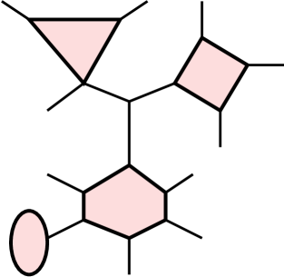
Figure 3.1. A graph with disjoint cycles. The cycles are emphasized by coloring the faces they bound.

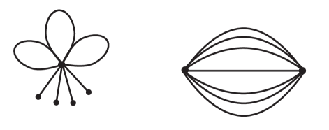
Figure 3.2. On the left, a stower graph with 3 loops and 4 tails. On the right, a mandarin graph with 7 edges.

The nodal surplus distribution for graphs with disjoint cycles was calculated in [5]:

Theorem 3.2.

[5] If $\Gamma_{{\boldsymbol{\ell}}}$ has disjoint cycles and rationally independent edge lengths, then its nodal surplus distribution is binomial with parameters $n=\beta$ and $p=\frac{1}{2}$. That is,

$$P(\sigma=s)=\binom{\beta}{s}2^{-\beta}.$$ (3.6)

Corollary 3.3.

The family of graphs with disjoint cycles satisfies Conjecture 3.1.

In contrast to this family of graphs, the cycles of stower graphs and mandarin graphs are clustered together such that every pair of cycles share an edge or a vertex. These are, in a sense, opposite to the case of disjoint cycles.

Theorem 3.4.

Both graph families of stowers and mandarins satisfy Conjecture 3.1.

We prove Theorem 3.4 in Section 7.

Remark 3.5.

Theorem 3.4 can be extended to include mandarin graphs with an added tail, but the proof is cumbersome and we do not include it here. Additionally, the methods used in the proof of Theorem 3.2 can be extended to graphs obtained by concatenation of small graphs.

3.2. Efficient computation of the nodal surplus distribution

The next theorem provides an efficient way to evaluate the nodal surplus distribution for large graphs. Given a graph $\Gamma$ with $E$ edges, its so-called bond scattering matrix $S$, explicitly defined in (4.1), is a $2E\times 2E$ constant real orthogonal matrix.

Definition 3.6.

The unitary evolution matrix associated to ${\vec{\kappa}}\in\mathbb{T}^{E}:=\mathbb{R}^{E}/2\pi\mathbb{Z}^{E}$ is defined by

$$U_{{\vec{\kappa}}}:=e^{i\hat{\kappa}}S,$$ (3.7)

where $e^{i\hat{\kappa}}$ is the diagonal matrix

$$e^{i\hat{\kappa}}:=\textrm{diag}\left(e^{i\kappa_{1}},e^{i\kappa_{2}}\ldots e^{i\kappa_{E}},e^{i\kappa_{1}},e^{i\kappa_{2}},\ldots e^{i\kappa_{E}}\right).$$

The eigenvalues and (orthonormal) eigenvectors of $U_{{\vec{\kappa}}}$ will be denoted by $e^{i\theta_{n}}({\vec{\kappa}})$ and $\boldsymbol{a}_{n}({\vec{\kappa}})$, for $1\leq n\leq 2E$. When ${\vec{\kappa}}$ is understood from the context, we simply write $e^{i\theta_{n}}$ and $\boldsymbol{a}_{n}$.

Given ${\vec{\kappa}}$ and an eigenpair $(e^{i\theta_{n}},\boldsymbol{a}_{n})$ of $U_{{\vec{\kappa}}}$, we construct $\boldsymbol{H}_{n}({\vec{\kappa}})$, an $E\times E$ real symmetric matrix whose signature is related to the nodal surplus, see Sections 5.1 and 5.2 for details. To be able to define $\boldsymbol{H}_{n}({\vec{\kappa}})$, we first introduce the self-adjoint matrix $g(e^{-i\theta_{n}}U_{{\vec{\kappa}}})$ given by

$$g(e^{-i\theta_{n}}U_{{\vec{\kappa}}})=\sum_{m\leq 2E~{};~{}e^{i\theta_{m}}\neq e^{i\theta_{n}}}\cot\left(\frac{\theta_{n}-\theta_{m}}{2}\right)\boldsymbol{a}_{m}\boldsymbol{a}_{m}^{*}.$$

The map $g$ which sends unitary matrices to self-adjoint matrices is defined in Section 5.2. We will remark that $g(M)$ agrees with the inverse Cayley transform of $M$ whenever defined. Next we define the matrices $Z_{j}$ for $j=1,2,\ldots,E$. Each $Z_{j}$ is a $2E$-dimensional matrix, with

$$(Z_{j})_{j,j}=-(Z_{j})_{j+E,j+E}=1,$$ (3.8)

and zero in all other entries. We define $\boldsymbol{H}_{n}({\vec{\kappa}})$ by

$$\left(\boldsymbol{H}_{n}({\vec{\kappa}})\right)_{j,j^{\prime}}:=\boldsymbol{a}_{n}^{*}Z_{j}g\left(e^{-i\theta_{n}}U_{{\vec{\kappa}}}\right)Z_{j^{\prime}}\boldsymbol{a}_{n},\qquad j,j^{\prime}\in\{1,\ldots,E\}.$$ (3.9)

Theorem 3.7.

Let $\Gamma$ be a graph with $E$ edges and first Betti number $\beta$. Assume $\Gamma$ has no loops. Then for any rationally independent ${\boldsymbol{\ell}}\in\mathbb{R}_{+}^{E}$, the nodal surplus distribution of $\Gamma_{{\boldsymbol{\ell}}}$ is given by

$$P\left(\sigma=s\right)=\frac{1}{(2\pi)^{E}}\int_{\mathbb{T}^{E}}\sum_{n=1}^{2E}I^{+}_{s}\big{(}\boldsymbol{H}_{n}({\vec{\kappa}})\big{)}\frac{\boldsymbol{a}_{n}^{*}\boldsymbol{L}\boldsymbol{a}_{n}}{\operatorname{tr}\boldsymbol{L}}\mathop{\mathrm{\mathstrut d}}\nolimits\!{\vec{\kappa}},$$ (3.10)

where $\boldsymbol{L}:=\textrm{diag}\left(l_{1},l_{2}\ldots l_{E},l_{1},l_{2},\ldots l_{E}\right)$ and the indicator function $I^{+}_{s}(H)$ is equal to 1 if the matrix $H$ has exactly $s$ positive eigenvalues and 0 otherwise.

The “no loops” assumption was introduced for readability only; the complete version of this result appears as Theorem 5.12 in section 5.3. We will also show that choice of the eigenvalue basis in the definition of $\boldsymbol{H}_{n}$ does not alter the integral in (3.10).

Remark 3.8.

The Cayley transform of a scattering matrix is related to the Dirichlet-to-Neumann map (see [17, eq. (5.4.8)] in the context of metric graphs). The appearance of an index such as $I^{+}_{s}\big{(}\boldsymbol{H}_{n}({\vec{\kappa}})\big{)}$ suggests links to the Cox–Jones–Marzuola formula for the nodal surplus in terms of the Morse index of the DtN map [28].

Theorem 3.7 is built upon two major ingredients:

1. A method, originated in [11] by Barra and Gaspard, that replaces certain spectral averages with integration over a hypersurface $\Sigma$ in the torus $\mathbb{T}^{E}$. In Theorem 4.10 we show that the integration over the implicitly defined $\Sigma$ can be replaced by an explicit integration over the torus $\mathbb{T}^{E}$, in the spirit of [20, 32].

2. A connection between the nodal surplus and eigenvalue stability with respect to certain perturbations, observed in [15, 23, 19], and its formulation as a function on the hypersurface $\Sigma$, [6, 5]. In sections 5.1 and 5.2 we compute this function explicitly in terms of the data used in the integral of Theorem 4.10.

3.3. The polytope of nodal surplus distributions of a given graph

Theorem 3.7 gives a computationally efficient way to calculate the nodal surplus for a given graph and a given choice of edge lengths. On the other hand, Conjecture 3.1 claims convergence for any sequence of graphs and almost any choice of lengths. We will now explain how to cover all choices of lengths for a given graph by testing only a few selected choices.

We note that the expression in the right-hand-side of (3.10) is well-defined for every non-zero ${\boldsymbol{\ell}}\in\mathbb{R}_{\geq 0}^{E}$. In particular, given $e$ we define $W_{e,s}$ by taking ${\boldsymbol{\ell}}$ with $\ell_{e}=1$ and zero elsewhere,

$$W_{e,s}:=\frac{1}{\left(2\pi\right)^{E}}\int_{\mathbb{T}^{E}}\sum_{n=1}^{2E}I^{+}_{s}\big{(}\boldsymbol{H}_{n}({\vec{\kappa}})\big{)}\frac{|(\boldsymbol{a}_{n})_{e}|^{2}+|(\boldsymbol{a}_{n})_{e+E}|^{2}}{2}\mathop{\mathrm{\mathstrut d}}\nolimits\!{\vec{\kappa}}.$$ (3.11)

This way, (3.10) may be written as a convex combination of $W_{e,s}$’s with weights given by the normalized edge lengths. Namely,

$$P(\sigma=s)=\frac{1}{L}\sum_{e\in\mathcal{E}}\ell_{e}W_{e,s},\qquad L:=\sum_{e\in\mathcal{E}}\ell_{e},$$ (3.12)

for rationally independent ${\boldsymbol{\ell}}$. The nodal surplus distribution of $\Gamma_{\boldsymbol{\ell}}$ is characterized by the vector $\vec{P_{\boldsymbol{\ell}}}\in\mathbb{R}_{\geq 0}^{\beta+1}$ of probabilities $P(\sigma=s)$, $s=0,\ldots,\beta$. The set of all such vectors for a given graph $\Gamma$ (and varying ${\boldsymbol{\ell}}$) satisfies

$$\overline{\left\{\vec{P_{\boldsymbol{\ell}}}\,\,:\,\,{\boldsymbol{\ell}}\in\mathcal{L}(\Gamma)\right\}}=\operatorname{conv}\left\{\vec{W}_{e}\,\,:\,\,e\in\mathcal{E}\right\},$$ (3.13)

where $\operatorname{conv}$ is the convex hull and $\vec{W}_{e}=(W_{e,0},W_{e,1},\ldots,W_{e,\beta})$ and the closure is with respect to the standard topology on $\mathbb{R}^{\beta+1}$. Thus to understand the set of all nodal surplus distributions of a given graph we only need to understand the extreme points $\vec{W}_{e}$. Furthermore, this task is often reduced by the presence of symmetries in the underlying (discrete) graph $\Gamma$. It will be shown in Theorem 6.4 that if $e_{1}$ and $e_{2}$ are related by a symmetry, then $\vec{W}_{e_{1}}=\vec{W}_{e_{2}}$. All of the above remains valid for graphs with loops after a small modification of equation (3.12), see equation (6.5).

We bound the ${\boldsymbol{\ell}}$ dependence in Conjecture 3.1 and equations (3.4)-(3.5) in terms of the extreme points of the convex hull. Introducing new random variables $\omega_{e}$ supported on $\{0,1,\ldots\beta\}$ with probabilities given by the vector $\vec{W}_{e}$, namely $P(\omega_{e}=s):=W_{e,s}$, we have the following.

Lemma 3.9.

Given a graph $\Gamma$, let $\varepsilon:=\sqrt{\frac{\max_{e\in\mathcal{E}}\operatorname{Var}(\omega_{e})}{\min_{e\in\mathcal{E}}\operatorname{Var}(\omega_{e})}}-1$. Then, for any ${\boldsymbol{\ell}}\in\mathcal{L}(\Gamma)$,

$$\min_{e\in\mathcal{E}}\operatorname{Var}(\omega_{e})\leq \operatorname{Var}(\sigma)\leq\max_{e\in\mathcal{E}}\operatorname{Var}(\omega_{e}),\quad\text{ and }$$ (3.14)

$$\sup_{{\boldsymbol{\ell}}\in\mathcal{L}(\Gamma)}d_{KS}(\sigma,N(\sigma))\leq \max_{e\in\mathcal{E}}d_{KS}(\omega_{e},N(\omega_{e}))+\varepsilon.$$ (3.15)

This lemma is proved in Appendix B. It follows that Conjecture 3.1 holds if the following two sufficient conditions hold:

1. the upper bound in (3.15) converges to zero in $\beta$ uniformly on $G(\beta)$, and

2. for every graph in $G(\beta)$ and any edge $e$ of that graph, $\operatorname{Var}(\omega_{e})$ is of order $\beta$.

We remark that these are actually necessary and sufficient conditions, however, we will not show that here. To show it, one needs to provide a lower bound on the supremum in equation (3.15), which can be done but the proof is cumbersome and we only need the upper bound in this work.

3.4. Numerical evidence in support of Conjecture 3.1

3.4.1. Setting

To provide supportive evidence for Conjecture 3.1, we compute, numerically, the bounds in (3.15) and (3.14) for $26$ different discrete graphs with first Betti number ranging between $\beta=6$ to $\beta=55$. These $26$ graphs that were chosen are

1. Complete graphs on $n$ vertices for $n\in\{5,6\ldots 12\}$.

2. Periodic ladder graphs, see Figure 3.3, of $n$ steps for $n\in\{6,10,14,18,22\}$.

3. Periodic square lattices of $n^{2}$ vertices (Cayley graphs of $\mathbb{Z}^{2}/n\mathbb{Z}^{2}$, see Figure 3.3) for $n\in\{4,5,6,7\}$.

4. Random $5$-regular graphs. We choose one graph at random (uniformly) out of all possible $5$-regular graphs of $n$ vertices for each $n\in\{12,14,16,18,20\}$.

5. Random Erdős-Rényi graphs with $n$ vertices: each pair of vertices is connected by an edge with probability $0.75$ independently of all others. We choose one random graph for each $n\in\{9,10,11,12\}$.

Remark 3.10.

We emphasize that in our experiments we sampled one graph from each class of random graphs of a given size. The distribution of a nodal-like quantity over an ensemble of random graphs of fixed size is a related but distinct problem, and we do not address it here. We also remark that the first Betti number of an Erdős-Rényi graph of size $n$ is random (but, in an appropriate sense, growing with $n$). Thus, the first Betti number assigned to each such graph, both in Figure 3.4 and Figure 3.5, was calculated after the random graph was generated.

Remark 3.11.

Computations of another family of graphs, which we do not present here, was suggested by the authors of [38] due to their constant spectral gap property. It includes the graphs in [38, fig. 13,e,f] and their $\mathcal{T}$ iteration (defined in [38]). These graphs were investigated and their data (variance and KS-distance) agreed with the data presented in Figure 3.5 and Figure 3.4.

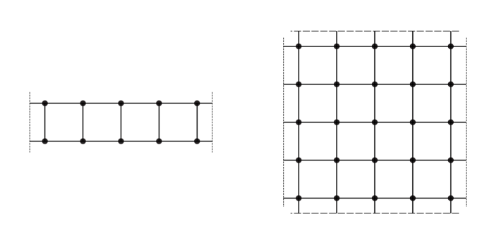
Figure 3.3. (left) Periodic ladder graph with $n=5$. (right) periodic square lattices of $n^{2}=5^{2}$ vertices. Dotted and dashed lines indicates gluing.

Given each of these graphs we compute its $\omega_{e}$’s as follows. We approximate the integral in (3.11) as

$$P(\omega_{e}=s)\approx\frac{\sum_{i=1}^{N}h({\vec{\kappa}}_{i})}{N},$$

with

$$h({\vec{\kappa}}):=\sum_{n=1}^{2E}I^{+}_{s}\big{(}\boldsymbol{H}_{n}({\vec{\kappa}})\big{)}\frac{|(\boldsymbol{a}_{n})_{e}|^{2}+|(\boldsymbol{a}_{n})_{e+E}|^{2}}{2},$$

by randomly sampling $N=\frac{10^{6}}{2E}$ points ${\vec{\kappa}}_{i}\in[0,2\pi]^{E}$ with uniform distribution. Heuristically, each sample provides the data of $2E$ eigenfunctions (see, for example, Theorem 4.10 and Remark 4.11), and so sampling $N=\frac{10^{6}}{2E}$ points provides the data of $10^{6}$ eigenfunctions. For a rigorous estimate of accuracy, we may apply Bernstein inequalities, by which the approximation error can be quantified as follows:

$$\forall\delta>0,\qquad P\left(\left|P(\omega_{e}=s)-\frac{\sum_{i=1}^{N}h({\vec{\kappa}}_{i})}{N}\right|>\delta\right)\leq 2e^{-N\frac{\delta^{2}}{2(1+\frac{\delta}{3})}}.$$

Another simplification is possible due to Theorem 6.4, which states that $\omega_{e}=\omega_{e^{\prime}}$ if $e$ and $e^{\prime}$ are related by a symmetry of the underlying discrete graph. In particular, in complete graphs and square lattices, every pair of edges can be related by a symmetry and so there is only one $\omega_{e}$ to compute.

We may estimate the running time of our algorithm as $O(NE^{3})$. To see that, note that we have $N$ iterations. In every iteration we first compute the eigenvalues and eigenvectors of $U_{{\vec{\kappa}}}$ at the cost $O(E^{3})$. Given the eigenvalues and eigenvectors of $U_{{\vec{\kappa}}}$, generating the $2E$ matrices $\boldsymbol{H}_{n}({\vec{\kappa}})$ is $O(E^{3})$ and computing their signature is $O(E^{3})$.

3.4.2. Experimental results

Our numerical results strongly support the conjecture. Figure 3.4 shows the upper bound (3.15) on $d_{KS}(\sigma,N(\sigma))$. The upper bound is presented as a function of $\beta$, and a uniform decrease can be observed as $\beta$ grows. Figure 3.5 shows $\operatorname{Var}(\omega_{e})$ for all graphs and all edges. The variance is presented as a function of $\beta$, and its linear growth is evident. All values obtained in the experiment satisfy

$$\frac{\beta}{10}\leq\operatorname{Var}(\omega_{e})\leq\frac{\beta}{5}.$$

In particular, all graphs in the experiment have variance smaller than $\beta/4$ which is the variance for graphs with disjoint cycles, by Theorem 3.2. We believe that $\frac{\beta}{4}$ should be the upper bound for all graphs.

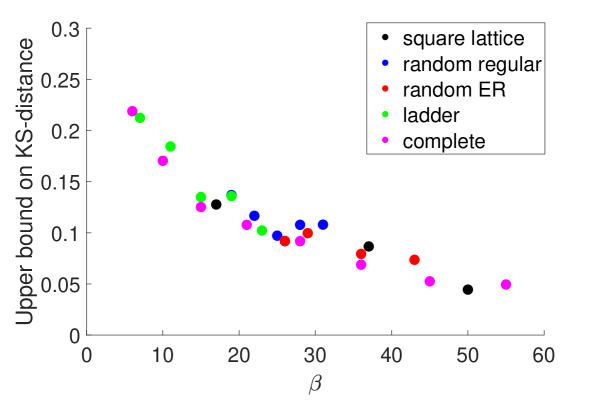
Figure 3.4. The upper bound, by (3.15), on $d_{KS}(\sigma,N(\sigma))$, as a function of the first Betti number $\beta$. Each point corresponds to a single graph. The colors of points indicate their family: (black) square lattices, (blue) 5-regular graphs, (red) Erdős-Rényi graphs, (green) ladder graphs and (magenta) complete graphs.

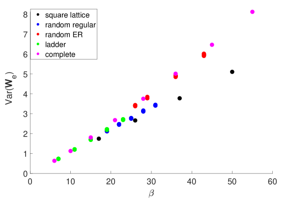
Figure 3.5. The variance, $\operatorname{Var}{(\omega_{e})}$, as a function of the first Betti number $\beta$. The points representing $\operatorname{Var}{(\omega_{e})}$, are plotted for each edge $e$ of every graph. In many cases, the differences between d$\operatorname{Var}{(\omega_{e})}$ for different edges are barely visible. The colors of points indicate their family: (black) square lattices, (blue) 5-regular graphs, (red) Erdős-Rényi graphs, (green) ladder graphs and (magenta) complete graphs.

The convergence of the $\omega_{e}$’s to Gaussian and the linear growth of their variance can also be seen in appendix C. There we show the full probability distribution of the “worst” $\omega_{e}$ for each graph considered. More precisely, we plot the $\omega_{e}$ which maximizes $d_{KS}\left(\omega_{e},N(\omega_{e})\right)$ among all edges of the graph.

Remark 3.12.

In this experiment we cover the nodal statistics of $26$ graphs, with $\beta$ ranging from $6$ to $55$ and $E$ ranging from $10$ to $98$. The efficiency of our algorithm using Theorem 3.7 is a major improvement over the direct computation of eigenfunctions and their zeros. For comparison, computing the first $10^{6}$ eigenfunctions of a graph with $E=10$ can take more than a day (for a given choice of edge lengths), while our algorithm will compute the nodal surplus statistics (for all rationally independent edge lengths) in a few minutes.

4. Secular averages

In this section we establish a new analytic expression for computing certain spectral averages of standard graphs with rationally independent lengths. In section 4.1 we recall that the spectrum of a standard graph is given as the roots of the characteristic (secular) equation or, equivalently, the intersection times of the secular manifold by a flow. Barra and Gaspard observed in [11] that since the flow is ergodic, some spectral averages may be computed by integrating over the secular manifold with a suitable measure, which we review in section 4.2. In section 4.3 we adapt this approach for more efficient numerical computation by replacing the integral over the (implicitly defined) secular manifold with an integral over the embedding torus. The main result of this section is Theorem 4.10.

4.1. The secular manifold

The discrete graphs $\Gamma$ we consider are undirected. An undirected graph $\Gamma$ can be made into a bi-directed graph by replacing each edge $e$ with two directed edges (sometimes called bonds) of opposite orientation. Given a directed edge $b$ we denote its reversed version by $\hat{b}$. We number the directed edges by $\{1,2,\ldots E,\hat{1},\hat{2}\ldots\hat{E}\}$. Let $i$ and $j$ be two directed edges such that $i$ terminates at a vertex $v$ and $j$ originates from a vertex $u$. If $u=v$ we write $i\xrightarrow[v]{}j$, otherwise we write $i\not\rightarrow{}j$. The bond scattering matrix, $S$, is a $2E\times 2E$ real orthogonal matrix defined as follows:

$$S_{j,i}=\begin{cases}\frac{2}{\mathrm{deg}(v)}&i\xrightarrow[v]{}j\,\,\,\text{and}\,\,i\neq\hat{j}\\ \frac{2}{\mathrm{deg}(v)}-1&i\xrightarrow[v]{}j\,\,\,\text{and}\,\,i=\hat{j}\\ 0&i\not\rightarrow{}j\end{cases}.$$ (4.1)

Recall our definition of the unitary evolution matrix, $U_{{\vec{\kappa}}}:=e^{i\hat{\kappa}}S$, associated to a point ${\vec{\kappa}}\in\mathbb{T}^{E}$ (see Definition 3.6).

Definition 4.1.

The secular manifold is the torus subset $\Sigma\subset\mathbb{T}^{E}$ for which $U_{{\vec{\kappa}}}$ has eigenvalue $1$. Namely,

$$\Sigma:=\left\{{\vec{\kappa}}\in\mathbb{T}^{E}\,\,:\,\,\det\left(1-U_{{\vec{\kappa}}}\right)=0\right\}.$$

Its set of regular points is defined as,

$$\Sigma^{\mathrm{reg}}:=\left\{{\vec{\kappa}}\in\Sigma\,\,:\,\,\nabla\det\left(1-U_{{\vec{\kappa}}}\right)\neq 0\right\},$$

and the set of singular points is $\Sigma^{\mathrm{sing}}:=\Sigma\setminus\Sigma^{\mathrm{reg}}$.

Remark 4.2.

The sets $\Sigma,\Sigma^{\mathrm{reg}}$ and $\Sigma^{\mathrm{sing}}$ can be characterized as the sets for which $\dim(\ker(1-U_{{\vec{\kappa}}}))\geq 1$, $\dim(\ker(1-U_{{\vec{\kappa}}}))=1$ and $\dim(\ker(1-U_{{\vec{\kappa}}}))>1$ correspondingly, [20, 25]. The regular part $\Sigma^{\mathrm{reg}}$ is an $E-1$ dimensional oriented smooth Riemannian manifold, [25].

We use the notation $\{{\vec{x}}\}_{2\pi}$ to denote the remainder, modulo $2\pi$, in each coordinate. The secular manifold $\Sigma$ can be used to compute the spectrum of the standard graphs $\Gamma_{{\boldsymbol{\ell}}}$ for any choice of ${\boldsymbol{\ell}}\in\mathbb{R}_{+}^{E}$.

Lemma 4.3.

[54, 41, 11, 25] Let $\Gamma$ be a graph and let $\Sigma$ be its secular manifold. Given a fixed choice of ${\boldsymbol{\ell}}\in\mathbb{R}_{+}^{E}$, the spectrum of $\Gamma_{{\boldsymbol{\ell}}}$ is characterized by

1. $k^{2}$ is an eigenvalue of $\Gamma_{{\boldsymbol{\ell}}}$ if and only if $\{k{\boldsymbol{\ell}}\}_{2\pi}$ lies in $\Sigma$.

2. A non-zero eigenvalue $k^{2}\neq 0$ is simple if $\{k{\boldsymbol{\ell}}\}_{2\pi}$ lies in $\Sigma^{\mathrm{reg}}$, and has multiplicity if $\{k{\boldsymbol{\ell}}\}_{2\pi}$ lies in $\Sigma^{\mathrm{sing}}$.

3. The singular set $\Sigma^{\mathrm{sing}}$ has positive co-dimension in $\Sigma$, $\dim(\Sigma^{\mathrm{sing}})\leq E-2$, and so the regular set $\Sigma^{\mathrm{reg}}$ has full measure in $\Sigma$.

Part (1) of the lemma, served as the motivation for constructing the secular manifold in [11], and was already deduced implicitly in [54, 41]. Parts (2) and (3) can be found in [25, Theorem 1.1].

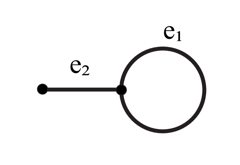
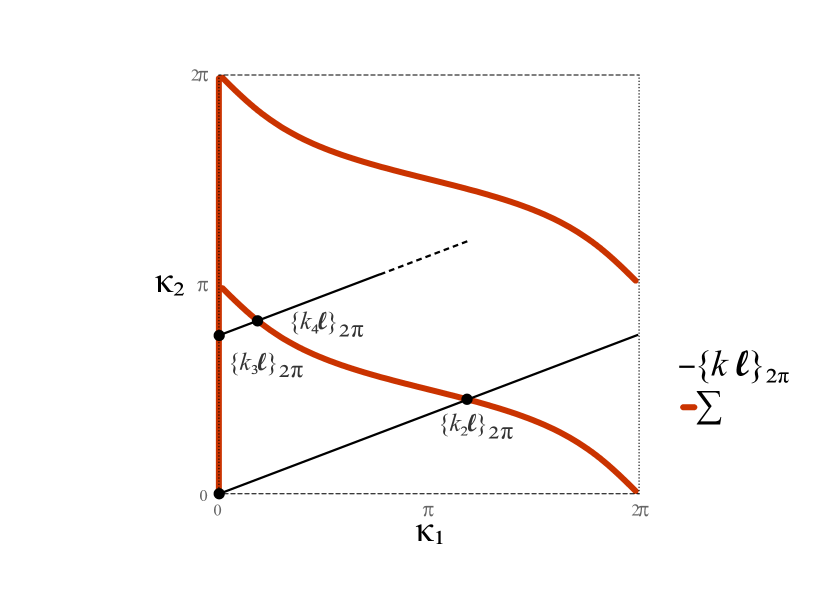
Figure 4.1. (left) a graph $\Gamma$ with two edges. (right) the secular manifold $\Sigma$ and the flow $k\mapsto\{k{\boldsymbol{\ell}}\}_{2\pi}$ intersecting it. There are two singular points $\Sigma^{\mathrm{sing}}=\{(0,\pi),(0,2\pi)\}$ (and their identifications).

The lemma is illustrated in Figure 4.1. The (discrete) graph $\Gamma$ determines the secular manifold $\Sigma$, while the lengths ${\boldsymbol{\ell}}$ determine the linear flow on the torus, $k\mapsto\{k{\boldsymbol{\ell}}\}_{2\pi}\in\mathbb{T}^{E}$. The (square-root) eigenvalues of $\Gamma_{{\boldsymbol{\ell}}}$, $\{k_{n}\}_{n\in\mathbb{N}}$, are the “hitting times” for which $\{k{\boldsymbol{\ell}}\}_{2\pi}\in\Sigma$. This simple but fruitful viewpoint was first introduced, in the context of quantum graphs, by Barra and Gaspard [11].

4.2. The Barra-Gaspard method

A spectral observable is a function on the eigenpairs $(k_{n},f_{n})$ of $\Gamma_{{\boldsymbol{\ell}}}$, which we denote by $\tilde{h}(\Gamma_{{\boldsymbol{\ell}}},k_{n},f_{n})$.

Definition 4.4.

We say that the spectral observable $\tilde{h}$ has an oracle function $h_{{\boldsymbol{\ell}}}:\Sigma\to\mathbb{R}$, if for every eigenpair $(k_{n},f_{n})$ of $\Gamma_{{\boldsymbol{\ell}}}$,

$$\tilde{h}(\Gamma_{{\boldsymbol{\ell}}},k_{n},f_{n})=h_{\boldsymbol{\ell}}\big{(}\{k_{n}{\boldsymbol{\ell}}\}_{2\pi}\big{)}.$$

Examples of observables having an oracle function include the eigenvalues spacing $n\mapsto(k_{n+1}-k_{n})$ discussed in [11], eigenfunction statistics [20, 25], band widths in the continuous spectrum of periodic graphs [7, 30] as well as the nodal surplus of $f_{n}$ [6, 5] and Neumann surplus [4]. Surprisingly, the oracles for the latter two cases (nodal surplus and Neumann surplus) do not depend on ${\boldsymbol{\ell}}$.

If $\tilde{h}$ has an oracle function $h_{\boldsymbol{\ell}}$, then its spectral average

$$\left\langle\tilde{h}\right\rangle:=\lim_{N\rightarrow\infty}\frac{1}{N}\sum_{n=1}^{N}\tilde{h}(\Gamma_{{\boldsymbol{\ell}}},k_{n},f_{n})=\lim_{N\rightarrow\infty}\frac{1}{N}\sum_{n=1}^{N}h_{{\boldsymbol{\ell}}}\big{(}\{k_{n}{\boldsymbol{\ell}}\}_{2\pi}\big{)},$$

can be replaced by an integral of $h_{{\boldsymbol{\ell}}}$ over $\Sigma$ with the appropriate measure called the Barra-Gaspard (BG) measure.

Definition 4.5.

[11, 20, 25] Let $\Gamma$ be a graph with secular manifold $\Sigma$ and let $\Sigma^{\mathrm{reg}}$ be its regular part. Denote the volume form (or volume measure) of $\Sigma^{\mathrm{reg}}$ by $\mathop{\mathrm{\mathstrut d}}\nolimits\!s$ and let $\hat{n}$ be the normal vector field of $\Sigma^{\mathrm{reg}}$, chosen to have non-negative entries. Then, for any ${\boldsymbol{\ell}}\in\mathbb{R}_{\geq 0}^{E}\setminus\{0\}$ the BG-measure $\mu_{{\boldsymbol{\ell}}}$ on $\Sigma$ is defined by $\mu_{{\boldsymbol{\ell}}}(\Sigma\setminus\Sigma^{\mathrm{reg}})=0$ and its density on $\Sigma^{\mathrm{reg}}$

$$\mathop{\mathrm{\mathstrut d}}\nolimits\!\mu_{{\boldsymbol{\ell}}}:=\frac{\pi}{L}\frac{1}{\left(2\pi\right)^{E}}(\hat{n}\cdot{\boldsymbol{\ell}})\mathop{\mathrm{\mathstrut d}}\nolimits\!s,$$ (4.2)

where $L=\sum_{e\in\mathcal{E}}\ell_{e}$ is the total length. In terms of differential forms, the density can be written as

$$\mathop{\mathrm{\mathstrut d}}\nolimits\!\mu_{{\boldsymbol{\ell}}}=\frac{\pi}{L}\frac{1}{\left(2\pi\right)^{E}}\sum_{j=1}^{E}(-1)^{j-1}\ell_{j}\,d\kappa_{1}\wedge d\kappa_{2}\ldots\wedge\widehat{d\kappa_{j}}\ldots\wedge d\kappa_{E},$$ (4.3)

where $\widehat{d\kappa_{j}}$ indicates that $d\kappa_{j}$ is omitted.

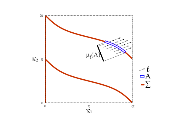
Figure 4.2. Illustration of a set $A\subset\Sigma$ and its BG-measure $\mu_{{\boldsymbol{\ell}}}(A)$. The arrows indicate the constant vector field ${\boldsymbol{\ell}}$.

Remark 4.6.

Up to a normalizing factor, the measure of $A\subset\Sigma$ is the flux across $A$ of the constant vector field in the direction ${\boldsymbol{\ell}}$. Equivalently, it is the “cross section” (in physics terminology) of $A$ as seen from the direction ${\boldsymbol{\ell}}$, see Figure 4.2. The normalization is chosen so that the BG-measures are Borel probability measures on $\Sigma$.

The next theorem states that for rationally independent ${\boldsymbol{\ell}}$, the discrete measures that average over the first $N$ points of $\left\{\{k_{n}{\boldsymbol{\ell}}\}_{2\pi}\right\}_{n\in\mathbb{N}}\subset\Sigma$ converge to $\mu_{\boldsymbol{\ell}}$ when $N\to\infty$.

Theorem 4.7.

[11, 20, 25] Let $\Gamma$ be a graph with secular manifold $\Sigma$. Let $\Gamma_{{\boldsymbol{\ell}}}$ be a standard graph with (square-root) eigenvalues $k_{n}$ for $n\in\mathbb{N}$. If ${\boldsymbol{\ell}}$ is rationally independent, then for any Riemann integrable $h:\Sigma\rightarrow\mathbb{C}$,

$$\lim_{N\rightarrow\infty}\frac{1}{N}\sum_{n=1}^{N}h\big{(}\{k_{n}{\boldsymbol{\ell}}\}_{2\pi}\big{)}=\int_{\Sigma}h\mathop{\mathrm{\mathstrut d}}\nolimits\!\mu_{{\boldsymbol{\ell}}}.$$ (4.4)

Although we are motivated by Theorem 4.7 which only applies to rationally independent ${\boldsymbol{\ell}}$’s, a prominent role will be played by the following measures with rational ${\boldsymbol{\ell}}$.

Definition 4.8.

Given $e\in\mathcal{E}$, let $\mu_{e}$ denote the BG-measure corresponding to ${\boldsymbol{\ell}}=(0,\ldots,1,\ldots,0)$, with 1 in the $e$-th position. We also use $\mu_{\boldsymbol{1}}$ to denote the BG-measure corresponding to ${\boldsymbol{\ell}}={\boldsymbol{1}}:=(1,\ldots,1)$.

As can be seen immediately from Definition 4.5, for any non-zero lengths ${\boldsymbol{\ell}}$,

$$\mu_{{\boldsymbol{\ell}}}=\frac{1}{L}\sum_{e\in\mathcal{E}}\ell_{e}\mu_{e}.$$ (4.5)

In other words, the set of all BG-measures is the convex hull of the $\mu_{e}$’s, and so has the structure of a finite convex polytope (with $n\leq E$ vertices). We may therefore interpret $\mu_{\boldsymbol{1}}=\frac{1}{E}\sum_{e\in\mathcal{E}}\mu_{e}$ as the average BG-measure (or the middle point of the polytope). We can also say that the BG-measures with rationally independent ${\boldsymbol{\ell}}$ are dense in the set of BG-measures (in the same way that the rationally independent points of a polytope in $\mathbb{R}^{n}$ are dense).

4.3. BG method as a torus integral

Theorem 4.7 provides an analytic tool to investigate spectral averages. However, an integral over an implicit high-dimensional hypersurface, such as $\Sigma$, may be harder to compute than the spectral average itself. For this reason we introduce Theorem 4.10 which describes the BG-measure in terms of the unitary evolution matrices, $U_{{\vec{\kappa}}}$ for ${\vec{\kappa}}\in{\mathbb{T}^{E}}$. Using this theorem, integrals against a BG-measure can be evaluated efficiently by sampling random points uniformly on $\mathbb{T}^{E}$. This is a new result, generalizing, in particular, [20, Thm. 3.4].

In what comes next, rather than talking about eigenvalues of unitary matrices $z=e^{it}$, where $e^{it}\in S^{1}:=\left\{z\in\mathbb{C}\,\,:\,\,|z|=1\right\}$, it will be more convenient to use their eigenphases $t\in\mathbb{T}:=\mathbb{R}/2\pi\mathbb{Z}$. We will also use the following notational convention.

Definition 4.9.

Consider the diagonal action of the abelian group $\mathbb{T}$ on $\mathbb{T}^{E}$ defined by

$$t\colon{\vec{\kappa}}\mapsto\{{\vec{\kappa}}+t{\boldsymbol{1}}\}_{2\pi},\qquad t\in\mathbb{T},$$ (4.6)

where ${\boldsymbol{1}}:=(1,1,\ldots)$. With a slight abuse of notation, we will denote this action simply as ${\vec{\kappa}}+t$. We denote the orbit of ${\vec{\kappa}}$ under this action by ${\vec{\kappa}}+\mathbb{T}$.

Combining the above notation with Definition 3.6 gives

$$U_{{\vec{\kappa}}-t}=e^{-it}U_{{\vec{\kappa}}}.$$ (4.7)

In particular, $e^{it}$ is an eigenvalue of $U_{{\vec{\kappa}}}$ if and only if 1 is an eigenvalue of $U_{{\vec{\kappa}}-t}$, yielding

$$e^{it}\text{ is an eigenvalue of }U_{{\vec{\kappa}}}\iff{\vec{\kappa}}-t\in\Sigma.$$ (4.8)

Theorem 4.10.

Let $\Gamma$ be a (discrete) graph and let ${\boldsymbol{\ell}}\in\mathbb{R}_{\geq 0}^{E}\setminus\{0\}$. At every ${\vec{\kappa}}\in\mathbb{T}^{E}$, denote the eigenphases and (orthonormal) eigenvectors of $U_{{\vec{\kappa}}}$ by $\theta_{n}({\vec{\kappa}})$ and $\boldsymbol{a}_{n}({\vec{\kappa}})$ for $n=1,2,\ldots,2E$. Then for any measurable $h:\Sigma\to\mathbb{C}$ we have

$$\int_{\Sigma}h\mathop{\mathrm{\mathstrut d}}\nolimits\!\mu_{{\boldsymbol{\ell}}}=\int_{\mathbb{T}^{E}}\sum_{n=1}^{2E}h\big{(}{\vec{\kappa}}-\theta_{n}\big{)}\frac{\boldsymbol{a}_{n}^{*}\boldsymbol{L}\boldsymbol{a}_{n}}{\operatorname{tr}(\boldsymbol{L})}\frac{\mathop{\mathrm{\mathstrut d}}\nolimits\!{\vec{\kappa}}}{(2\pi)^{E}},$$ (4.9)

where the ${\vec{\kappa}}$ dependence of $\theta_{n}$ and $\boldsymbol{a}_{n}$ is omitted for brevity and $\boldsymbol{L}:=\emph{{diag}}({\boldsymbol{\ell}},{\boldsymbol{\ell}})$.

Remark 4.11.

The integrand in the right-hand-side of (4.9) is a weighted average of $h$ over the intersection points $\{{\vec{\kappa}}+\mathbb{T}\}\cap\Sigma=\{{\vec{\kappa}}-\theta_{n}\}_{n=1}^{2E}$, see Figure 4.4 for example. Implicit in (4.9) is the claim that the integrand is measurable on $\mathbb{T}^{E}$.

Remark 4.12.

Consider the spectral decomposition of $U_{\vec{\kappa}}$,

$$U_{{\vec{\kappa}}}=\sum_{e^{i\theta}\in\operatorname{spec}(U_{{\vec{\kappa}}})}e^{i\theta}P_{\theta},$$

where the sum is over distinct eigenvalues $e^{i\theta}$ of $U_{\vec{\kappa}}$ and $P_{\theta}$ is the spectral projection, i.e. the orthogonal projection onto the eigenspaces $\ker(e^{i\theta}-U_{{\vec{\kappa}}})$. In this form, Theorem 4.10 can be stated as

$$\int_{\Sigma}h\mathop{\mathrm{\mathstrut d}}\nolimits\!\mu_{{\boldsymbol{\ell}}}=\int_{\mathbb{T}^{E}}\sum_{e^{i\theta}\in\operatorname{spec}(U_{{\vec{\kappa}}})}h\big{(}{\vec{\kappa}}-\theta({\vec{\kappa}})\big{)}\frac{\operatorname{tr}\big{(}P_{\theta}({\vec{\kappa}})\boldsymbol{L}\big{)}}{\operatorname{tr}(\boldsymbol{L})}\frac{\mathop{\mathrm{\mathstrut d}}\nolimits\!{\vec{\kappa}}}{(2\pi)^{E}}$$ (4.10)

which highlights its independence of the numbering of eigenphases and the choice of the eigenvectors.

The proof of Theorem 4.10 will be partitioned into two steps. The first step would be to establish the Theorem for one particular BG-measure, $\mu_{\textbf{1}}$ with ${\boldsymbol{\ell}}=\textbf{1}:=(1,1,1\ldots)$. The second step would be to extend this result to every $\mu_{{\boldsymbol{\ell}}}$ by calculating the Radon-Nikodym derivative of $\mu_{{\boldsymbol{\ell}}}$ with respect to $\mu_{\textbf{1}}$.

To study the integral over $\Sigma$, we will partition $\Sigma$ into “layers”, with the $n$-th layer defined as the set of ${\vec{\kappa}}\in\mathbb{T}^{E}$ where the $n$-th eigenvalue of $U_{\vec{\kappa}}$ is equal to 1. However, as can be seen from Proposition A.4, the eigenvalues cannot be ordered counterclockwise continuously throughout $\mathbb{T}^{E}$. This fact necessitates the following construction.

Let $X=\left[0,2\pi\right)^{E-1}$ which we will identify with the subset $\{{\vec{\kappa}}\in\mathbb{T}^{E}:\kappa_{E}=0\}$ of $\mathbb{T}^{E}$ via the mapping ${\vec{x}}\in X\mapsto({\vec{x}},0)\in\mathbb{T}^{E}$. Note that we do not identify the sides of the cube $X$. In a slight abuse of notation we will write $U_{\vec{x}}$ with ${\vec{x}}\in X$ instead of $U_{({\vec{x}},0)}$ and will use a similar shorthand for the eigenphases and eigenvectors of $U_{({\vec{x}},0)}$.

We define the diagonal projection $\mathrm{p}:\mathbb{T}^{E}\to X$ by

$$\mathrm{p}:(\kappa_{1},\kappa_{2},\ldots,\kappa_{E})\mapsto(\kappa_{1}-\kappa_{E},\kappa_{2}-\kappa_{E},\ldots,\kappa_{E-1}-\kappa_{E}),$$ (4.11)

see Figure 4.4 for illustration. By definition of the matrix $U_{\vec{\kappa}}$, see (3.7), we have

$$U_{\vec{\kappa}}=e^{i\kappa_{E}}U_{\mathrm{p}({\vec{\kappa}})},$$ (4.12)

Therefore, $U_{\vec{\kappa}}$ and $U_{\mathrm{p}({\vec{\kappa}})}$ share the same eigenspaces and their eigenphases are related by a shift by $\kappa_{E}$. More precisely, $\boldsymbol{a}$ is an eigenvector of $U_{\mathrm{p}({\vec{\kappa}})}$ with eigenvalue $e^{i\theta}$ if and only if $\boldsymbol{a}$ is an eigenvector of $U_{\vec{\kappa}}$ with eigenvalue $e^{i(\theta+\kappa_{E})}$.

Lemma 4.13.

Consider a graph $\Gamma$ of $E$ edges. There exist continuous functions $\theta_{n}\colon X\to\mathbb{T}$, $n=1,\ldots,E$, such that the spectrum of $U_{\vec{x}}$ for any ${\vec{x}}\in X$ is given by $\operatorname{spec}(U_{\vec{x}})=\left\{e^{i\theta_{n}({\vec{x}})}\right\}_{n=1}^{E}$. When $e^{i\theta_{n}({\vec{x}})}$ is a simple eigenvalue, $\theta_{n}({\vec{x}})$ and its corresponding eigenvector $\boldsymbol{a}_{n}({\vec{x}})$ are analytic in some neighborhood of ${\vec{x}}$.

Proof.

The family $U_{{\vec{x}}}$ is analytic in ${\vec{x}}$, and the domain $X$ is simply connected, therefore the lemma is a direct consequence of Propostion A.4 of Appendix A, as well as classical results of perturbation theory [51]. ∎

Using relation (4.12), we extend the functions $\theta_{n}$ from $X$ to the whole of $\mathbb{T}^{E}$,

$$\theta_{n}:\mathbb{T}^{E}\to\mathbb{T}\qquad\theta_{n}({\vec{\kappa}}):=\theta_{n}\big{(}\mathrm{p}({\vec{\kappa}})\big{)}+\kappa_{E},\qquad{\vec{\kappa}}=(\kappa_{1},\ldots,\kappa_{E}).$$ (4.13)

Consequently, the spectrum of $U_{\vec{\kappa}}$ for any ${\vec{\kappa}}\in\mathbb{T}^{E}$ is given by

$$\operatorname{spec}(U_{\vec{\kappa}})=\left\{e^{i\theta_{n}({\vec{\kappa}})}\right\}_{n=1}^{E}.$$ (4.14)

Note that $\theta_{n}$ are continuous only on $\mathbb{T}^{E}\setminus\partial\Omega$, where $\Omega$ is the embedding of $X\times\mathbb{T}$ into $\mathbb{T}^{E}$ (see Figure 4.5 for example) and

$$\partial\Omega:=\{{\vec{\kappa}}\in\mathbb{T}^{E}\colon\kappa_{j}=\kappa_{E}\text{ for some }j,\ 1\leq j\leq E-1\}.$$

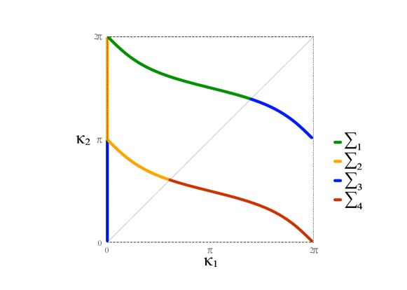
Figure 4.3. A secular manifold colored according to its layers $\Sigma_{n}$. Here $\partial\Omega$ is the diagonal line $\kappa_{1}=\kappa_{2}$. The coloring is discontinuous on $\partial\Omega$ and the singular points $\Sigma^{\mathrm{sing}}=\{(0,\pi),(0,2\pi)\}$ (and their identifications).

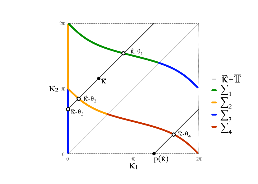
Figure 4.4. A point ${\vec{\kappa}}\in\mathbb{T}^{2}$ and its diagonal orbit ${\vec{\kappa}}+\mathbb{T}$. The (embedding of the) point $\mathrm{p}({\vec{\kappa}})$ is presented and the intersection points $\{{\vec{\kappa}}+\mathbb{T}\}\cap\Sigma=\{{\vec{\kappa}}-\theta_{1},\ldots,{\vec{\kappa}}-\theta_{4}\}$ are shown to match the layer structure numbering.

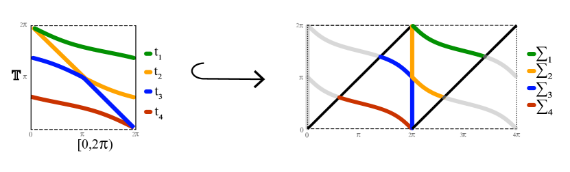
Figure 4.5. The embedding $[0,2\pi)\times\mathbb{T}\hookrightarrow\mathbb{T}^{2}$. (left) $[0,2\pi)\times\mathbb{T}$. The graphs of the functions $t_{n}({\vec{x}})=-\theta_{n}({\vec{x}})$ are displayed in different colors. (right) Illustration of $\Omega$, the embedding of $[0,2\pi)\times\mathbb{T}$ into $\mathbb{T}^{2}$, with black margins indicating the boundary $\partial\Omega$. The layers $\Sigma_{n}$, coming from the graphs of $t_{n}$, are displayed in different colors.

Lemma 4.14.

With $\theta_{n}:\mathbb{T}^{E}\to\mathbb{T}$ defined by (4.13), let

$$\Sigma_{n}:=\left\{{\vec{\kappa}}\in\mathbb{T}^{E}\,\,:\,\,e^{i\theta_{n}({\vec{\kappa}})}=1\right\},\qquad n=1,2,\ldots,2E.$$ (4.15)

Then $\Sigma_{n}$ have the following properties.

1. $$\Sigma=\bigcup_{n=1}^{2E}\Sigma_{n},\qquad\mbox{and}\qquad\Sigma^{\mathrm{sing}}=\bigcup_{1\leq{m}<n\leq{2E}}\Sigma_{n}\cap\Sigma_{m}.$$ (4.16)

2. The map

   $${\vec{\kappa}}_{n}({\vec{x}}):=({\vec{x}},0)-\theta_{n}({\vec{x}}),$$ (4.17)

   is a bijection $X\to\Sigma_{n}$ which is is differentiable except possibly for a set of positive co-dimension in $X$.

3. For any measurable $h$ on $\Sigma_{n}$,

   $$\int_{\Sigma_{n}}h\mathop{\mathrm{\mathstrut d}}\nolimits\!\mu_{\textbf{1}}=\frac{1}{2E}\int_{{\vec{x}}\in X}h({\vec{\kappa}}_{n}({\vec{x}}))\frac{\mathop{\mathrm{\mathstrut d}}\nolimits\!{\vec{x}}}{(2\pi)^{E-1}}.$$ (4.18)

   Namely, the push forward of the Lebesgue measure on $X=\left[0,2\pi\right)^{E-1}$ by ${\vec{\kappa}}_{n}$ is the restriction of the BG-measure $\mu_{\textbf{1}}$ to $\Sigma_{n}$, up to normalization.

See Figure 4.3 for an example of the layer structure given by (4.16), and Figure 4.5 for the construction of the Layer structure by embedding $X\times\mathbb{T}$ into $\mathbb{T}^{E}$.

Proof.

The first part follows immediately from (4.14) and Remark 4.2.

To show the second part we combine (4.15) and (4.13): the latter can be rewrtten as

$$\theta_{n}\big{(}({\vec{x}},0)+\kappa_{E}\big{)}=\theta_{n}({\vec{x}})+\kappa_{E},$$

which is equal to 0 if and only if $\kappa_{E}=-\theta_{n}({\vec{x}})\in\mathbb{T}$. The inverse of ${\vec{\kappa}}_{n}$ is the projection $\mathrm{p}$: $\mathrm{p}({\vec{\kappa}}_{n}({\vec{x}}))={\vec{x}}$. The map ${\vec{\kappa}}_{n}$ may not be differentiable at ${\vec{x}}$ if $\theta_{n}({\vec{x}})$ is not differentiable there, which can only happen if $e^{i\theta_{n}({\vec{x}})}$ is a multiple eigenvalue. The set of such ${\vec{x}}$ is obtained by projecting $\Sigma^{\mathrm{sing}}\cap\Sigma_{n}$ to $X$ by $\mathrm{p}$. Positive co-dimension of $\mathrm{p}(\Sigma^{\mathrm{sing}}\cap\Sigma_{n})$ in $X$ follows from

$$\dim(\mathrm{p}(\Sigma^{\mathrm{sing}}\cap\Sigma_{n}))\leq\dim(\Sigma^{\mathrm{sing}}\cap\Sigma_{n})\leq\dim(\Sigma^{\mathrm{sing}})\leq E-2,$$

where the last inequality is stated in Lemma 4.3.

To prove (4.18) we consider ${\vec{\kappa}}_{n}({\vec{x}})$ as a parameterization of $\Sigma_{n}$ by $X$. We claim that wherever it is differentiable, the parameterization ${\vec{\kappa}}={\vec{\kappa}}_{n}({\vec{x}})$ satisfies the identity

$$\sum_{j=1}^{E}(-1)^{j}\left|\frac{\partial\left(\kappa_{1},\kappa_{2},\ldots,\widehat{\kappa_{j}},\ldots,\kappa_{E}\right)}{\partial\left(x_{1},x_{2},\ldots,x_{E-1}\right)}\right|=1.$$ (4.19)

We will now prove (4.18) assuming (4.19) and will provide the proof of (4.19) later.

The density of the BG measure $\mu_{\textbf{1}}$ (as described in (4.3)) can be written in terms of ${\vec{\kappa}}={\vec{\kappa}}_{n}({\vec{x}})$ as

$$d\mu_{\textbf{1}} =\frac{\pi}{E}\frac{1}{(2\pi)^{E}}\sum_{j=1}^{E}(-1)^{j-1}d\kappa_{1}\wedge d\kappa_{2}\wedge\cdots\widehat{d\kappa_{j}}\cdots\wedge d\kappa_{E}$$

$$=\frac{1}{2E}\frac{1}{(2\pi)^{E-1}}\sum_{j=1}^{E}(-1)^{j-1}\left|\frac{\partial\left(\kappa_{1},\kappa_{2},\ldots,\widehat{\kappa_{j}},\ldots,\kappa_{E}\right)}{\partial\left(x_{1},x_{2},\ldots,x_{E-1}\right)}\right|dx_{1}\wedge dx_{2}\wedge\cdots\wedge dx_{E-1}$$

$$=\frac{1}{2E}\frac{1}{(2\pi)^{E-1}}dx_{1}\wedge dx_{2}\wedge\cdots\wedge dx_{E-1},$$

where in the last equality we used the identity (4.19). This establishes (4.18).

Let us prove identity (4.19). Let $D{\vec{\kappa}}_{n}({\vec{x}})$ be the $E\times E-1$ matrix of derivatives of ${\vec{\kappa}}_{n}({\vec{x}})$, and construct $M$, an $E\times E$ matrix, by adding to $D{\vec{\kappa}}_{n}({\vec{x}})$ an auxiliary column of ones, so that

$$\det(M)=\sum_{j=1}^{E}(-1)^{j}\left|\frac{\partial\left(\kappa_{1},\kappa_{2},\ldots,\widehat{\kappa_{j}},\ldots,\kappa_{E}\right)}{\partial\left(x_{1},x_{2},\ldots,x_{E-1}\right)}\right|,$$

by expansion of the determinant over the column of ones. To prove identity (4.19) we need to show that $\det(M)=1$. The derivatives of ${\vec{\kappa}}_{n}({\vec{x}})$ are

$$\frac{\partial\kappa_{i}}{\partial x_{j}}=\delta_{i,j}+\frac{\partial\theta_{n}({\vec{x}})}{\partial x_{j}},\qquad i=1,\ldots,E,\quad j=1,\ldots,E-1,$$ (4.20)

so $M$ is given by

$$M=\begin{pmatrix}1+\frac{\partial\theta_{n}}{\partial x_{1}}&\frac{\partial\theta_{n}}{\partial x_{2}}&\cdots&1\\[4.0pt] \frac{\partial\theta_{n}}{\partial x_{1}}&1+\frac{\partial\theta_{n}}{\partial x_{2}}&\cdots&1\\ \vdots&\vdots&&\vdots\\ \frac{\partial\theta_{n}}{\partial x_{1}}&\frac{\partial\theta_{n}}{\partial x_{2}}&\cdots&1\end{pmatrix}.$$ (4.21)

To see that the determinant of this matrix is 1 subtract the last row from all others. ∎

We may now use Lemma 4.14 to prove Theorem 4.10.

Proof of Theorem 4.10.

We start with the special case ${\boldsymbol{\ell}}=(1,\ldots,1)$ when $\boldsymbol{L}=\textrm{diag}({\boldsymbol{\ell}},{\boldsymbol{\ell}})$ is the identity matrix, and so the factor

$$\frac{\boldsymbol{a}_{n}({\vec{\kappa}})^{*}\boldsymbol{L}\boldsymbol{a}_{n}({\vec{\kappa}})}{\operatorname{tr}(\boldsymbol{L})}\equiv\frac{1}{2E},$$

is independent of ${\vec{\kappa}}$, due to $\|\boldsymbol{a}_{n}\|=1$. In this case, equation (4.9) reduces to

$$\int_{\Sigma}h\mathop{\mathrm{\mathstrut d}}\nolimits\!\mu_{\textbf{1}}=\int_{\mathbb{T}^{E}}\frac{1}{2E}\sum_{n=1}^{2E}h\big{(}{\vec{\kappa}}-\theta_{n}\big{)}\frac{\mathop{\mathrm{\mathstrut d}}\nolimits\!{\vec{\kappa}}}{(2\pi)^{E}}.$$ (4.22)

Focusing on one term in the sum on the right hand side, we have

$$\frac{1}{2E}\int_{\mathbb{T}^{E}}h\big{(}{\vec{\kappa}}-\theta_{n}\big{)}\frac{\mathop{\mathrm{\mathstrut d}}\nolimits\!{\vec{\kappa}}}{(2\pi)^{E}}=\frac{1}{2E}\int_{t\in\mathbb{T}}\int_{{\vec{x}}\in X}h\Big{(}{\vec{\kappa}}({\vec{x}},t)-\theta_{n}\big{(}{\vec{\kappa}}({\vec{x}},t)\big{)}\Big{)}\frac{\mathop{\mathrm{\mathstrut d}}\nolimits\!{\vec{x}}\mathop{\mathrm{\mathstrut d}}\nolimits\!t}{(2\pi)^{E}},$$ (4.23)

where we made the substitution ${\vec{\kappa}}({\vec{x}},t):=({\vec{x}},0)+t$ which has Jacobian equal to $1$ (the latter is an easy observation). For every $t\in\mathbb{T}$ and ${\vec{x}}\in X$ we have

$${\vec{\kappa}}({\vec{x}},t)-\theta_{n}({\vec{\kappa}}({\vec{x}},t))=({\vec{x}},0)+t-\big{(}\theta_{n}({\vec{x}})+t\big{)}=({\vec{x}},0)-\theta_{n}({\vec{x}})={\vec{\kappa}}_{n}({\vec{x}}),$$

where ${\vec{\kappa}}_{n}({\vec{x}})$ was introduced in Lemma 4.14. In particular, the integrand of the right hand side of (4.23) is independent of $t$. Integrating $t$ out, we obtain

$$\frac{1}{2E}\int_{\mathbb{T}^{E}}h\big{(}{\vec{\kappa}}-\theta_{n}\big{)}\frac{\mathop{\mathrm{\mathstrut d}}\nolimits\!{\vec{\kappa}}}{(2\pi)^{E}}=\frac{1}{2E}\int_{{\vec{x}}\in X}h\big{(}{\vec{\kappa}}_{n}({\vec{x}})\big{)}\frac{\mathop{\mathrm{\mathstrut d}}\nolimits\!{\vec{x}}}{(2\pi)^{E-1}}=\int_{\Sigma_{n}}h\mathop{\mathrm{\mathstrut d}}\nolimits\!\mu_{\textbf{1}},$$

where we applied Lemma 4.14 in the last step.

Finally, the summation of $\Sigma_{n}$ integrals is an integral over $\Sigma$ since the layers cover $\Sigma$ and intersect on $\Sigma^{\mathrm{sing}}$ (Lemma 4.14) which has measure zero (Lemma 4.3). To conclude, we have established (4.9) for $\mu_{\textbf{1}}$.

To prove (4.9) for $\mu_{{\boldsymbol{\ell}}}$ with arbitrary ${\boldsymbol{\ell}}$, of total length $L=\sum_{j=1}^{E}\ell_{j}$, we use

$$\int_{\Sigma}h\mathop{\mathrm{\mathstrut d}}\nolimits\!\mu_{{\boldsymbol{\ell}}}=\int_{\Sigma^{\mathrm{reg}}}h\mathop{\mathrm{\mathstrut d}}\nolimits\!\mu_{{\boldsymbol{\ell}}}=\int_{\Sigma^{\mathrm{reg}}}h\left|\frac{\hat{n}\cdot{\boldsymbol{\ell}}}{\hat{n}\cdot{\boldsymbol{1}}}\right|\frac{E}{L}d\mu_{\textbf{1}}.$$ (4.24)

The first equality is due to $\Sigma^{\mathrm{reg}}$ being a full measure subset, by Lemma 4.3. In the second equality we used Definition 4.5 to compute the Radon–Nikodym derivative of $\mu_{{\boldsymbol{\ell}}}$ with respect to $\mu_{{\boldsymbol{1}}}$ on $\Sigma^{\mathrm{reg}}$. According to [25, Thm. 1.1], the normal vector $\hat{n}$ at a regular point ${\vec{\kappa}}\in\Sigma^{\mathrm{reg}}$ is related to $\boldsymbol{a}$, the normalized eigenvector of eigenvalue 1 of $U_{\vec{\kappa}}$, by

$$\hat{n}_{e}\propto\left|\boldsymbol{a}_{e}\right|^{2}+\left|\boldsymbol{a}_{\hat{e}}\right|^{2}.$$

It follows, using the normalization $\|\boldsymbol{a}\|=1$, that

$$\left|\frac{\hat{n}\cdot{\boldsymbol{\ell}}}{\hat{n}\cdot{\boldsymbol{1}}}\right|=\frac{\sum_{e}\ell_{e}\left(\left|\boldsymbol{a}_{e}\right|^{2}+\left|\boldsymbol{a}_{\hat{e}}\right|^{2}\right)}{\sum_{e}\left(\left|\boldsymbol{a}_{e}\right|^{2}+\left|\boldsymbol{a}_{\hat{e}}\right|^{2}\right)}=\frac{\boldsymbol{a}^{*}\boldsymbol{L}\boldsymbol{a}}{\|\boldsymbol{a}\|^{2}}=\boldsymbol{a}^{*}\boldsymbol{L}\boldsymbol{a}.$$

Recall that if ${\vec{\kappa}}\in\Sigma_{n}\cap\Sigma^{\mathrm{reg}}$ then the normalized eigenvector of the simple eigenvalue $1$ is $\boldsymbol{a}_{n}({\vec{\kappa}})$ which is analytic for every ${\vec{\kappa}}\notin\partial\Omega$ around that point by Lemma 4.13. Finally, we represent $2L=\operatorname{tr}(\boldsymbol{L})$, so that

$$\int_{\Sigma}h\mathop{\mathrm{\mathstrut d}}\nolimits\!\mu_{{\boldsymbol{\ell}}}=2E\int_{\Sigma^{\mathrm{reg}}}h({\vec{\kappa}})\frac{\boldsymbol{a}_{n}({\vec{\kappa}})^{*}\boldsymbol{L}\boldsymbol{a}_{n}({\vec{\kappa}})}{\operatorname{tr}(\boldsymbol{L})}d\mu_{\textbf{1}}.$$

The theorem now follows by applying (4.22) to the measurable function

$${\vec{\kappa}}\mapsto h({\vec{\kappa}})\frac{\boldsymbol{a}_{n}({\vec{\kappa}})^{*}\boldsymbol{L}\boldsymbol{a}_{n}({\vec{\kappa}})}{\operatorname{tr}(\boldsymbol{L})},$$

and replacing $\boldsymbol{a}_{n}({\vec{\kappa}}-\theta_{n})$ with $\boldsymbol{a}_{n}({\vec{\kappa}})$, see (4.12) and the discussion following it. ∎

5. The nodal surplus distribution

The purpose of this section is to prove Theorem 3.7 and its generalization to graphs with loops, Theorem 5.12. These theorems are established in section 5.3 by applying Theorems 4.7 and 4.10 to a suitably defined oracle function $\boldsymbol{\sigma}:\Sigma\rightarrow\{0,1,\ldots\beta\}$ which encodes the nodal surplus on the secular manifold. More precisely, the function $\boldsymbol{\sigma}$ has the following properties:

1. It is Riemann integrable.

2. For any ${\boldsymbol{\ell}}\in\mathbb{R}_{+}^{E}$ and any $k_{n}$ eigenvalue of $\Gamma_{{\boldsymbol{\ell}}}$ with $n\in\mathcal{G}$, the nodal surplus equals:

   $$\sigma(n)=\boldsymbol{\sigma}\big{(}\{k_{n}{\boldsymbol{\ell}}\}_{2\pi}\big{)}.$$

Such a function was constructed in [5, 6], but in section 5.1 we give an alternative definition in terms of the Hessian of an eigenphase $\theta$ of $U_{{\vec{\kappa}}}$ and, in section 5.2, express the Hessian in terms of the corresponding eigenvector $\boldsymbol{a}$ and the inverse Cayley transform of $e^{-i\theta}U_{{\vec{\kappa}}}$.

5.1. The nodal surplus oracle function

In this section we describe the nodal surplus function $\boldsymbol{\sigma}:\Sigma\rightarrow{\{0,1,\ldots\beta\}}$, originally introduced in [5, 6], and express it in terms of the layers and eigenphases, introduced in Lemma 4.14. This will make $\boldsymbol{\sigma}$ compatible with Theorem 4.10.

To give a preview, the function $\boldsymbol{\sigma}$ is constructed as follows. We introduce an extra set of parameters $\vec{\alpha}$ in the definition of the unitary evolution matrix $U=U_{{\vec{\kappa}};\vec{\alpha}}$, see Definition 5.2 below. According to a theorem known as the “Nodal–Magnetic Connection”, established in [15, 24, 19] and quoted below as Theorem 5.5, the nodal surplus can be recovered by counting the negative eigenvalues of the matrix of second derivatives of the eigenphase $\theta$ of $U$ as a function of $\vec{\alpha}$. We remark that the word “magnetic” appears in the name of the theorem because the parameters $\vec{\alpha}$ can be understood as the fluxes in a magnetic Schrödinger operator. It can equivalently be viewed as twisting the graph Laplacian by the characters of its homology group [48]. However, neither interpretation will be particularly important in our calculations below.

To put this discussion on a rigorous basis, recall that the nodal surplus is defined only for generic eigenfunctions, see Definition 2.2. We now describe the submanifold $\Sigma^{\mathcal{G}}\subset\Sigma$ corresponding to such eigenfunctions.

Lemma 5.1.

[5] Given a graph $\Gamma$, there is a sub-manifold $\Sigma^{\mathcal{G}}\subset\Sigma^{\mathrm{reg}}$ such that for every ${\boldsymbol{\ell}}\in\mathbb{R}_{+}^{E}$, the index set $\mathcal{G}$ of $\Gamma_{{\boldsymbol{\ell}}}$ is characterized by

$$n\in\mathcal{G}\iff\{k_{n}{\boldsymbol{\ell}}\}_{2\pi}\in\Sigma^{\mathcal{G}}.$$ (5.1)

If $\Gamma$ has no loops, then $\Sigma^{\mathcal{G}}$ has full measure in $\Sigma$. If $\Gamma$ has loops, then

$$\mu_{{\boldsymbol{\ell}}}\left(\Sigma^{\mathcal{G}}\right)=1-\frac{L_{\textrm{loops}}}{2L},$$ (5.2)

where $L$ is the total length of $\Gamma_{{\boldsymbol{\ell}}}$ and $L_{\textrm{loops}}$ is the total length of its loops.

Definition 5.2.

For a given $\vec{\alpha}\in\mathbb{T}^{E}$ we define

$$e^{i\check{\alpha}}:=\textrm{diag}\left(e^{i\alpha_{1}},e^{i\alpha_{2}}\ldots e^{i\alpha_{E}},e^{-i\alpha_{1}},e^{-i\alpha_{2}},\ldots e^{-i\alpha_{E}}\right)$$ (5.3)

and further denote

$$U_{{\vec{\kappa}};\vec{\alpha}}:=e^{i\check{\alpha}}U_{{\vec{\kappa}}}=e^{i\check{\alpha}}e^{i\hat{\kappa}}S,$$ (5.4)

such that the unitary evolution matrix defined previously in (3.7) is given as $U_{{\vec{\kappa}}}:=U_{{\vec{\kappa}};0}$.

Remark 5.3.

Notice that the $j$-th and $(j+E)$-th diagonal elements of $e^{i\check{\alpha}}$ are conjugate rather than equal, in contrast to $e^{i\hat{\kappa}}$.

Consider the eigenphases of $U_{{\vec{\kappa}}}$ for every ${\vec{\kappa}}\in\mathbb{T}^{E}$, as defined in (4.13)

$$\theta_{m}:\mathbb{T}^{E}\to\mathbb{T},\qquad m=1,2,\ldots,2E.$$

Notice that $\det(U_{{\vec{\kappa}};\vec{\alpha}})=\det(U_{{\vec{\kappa}};0})=\det(U_{{\vec{\kappa}}})$, since $\det(e^{i\check{\alpha}})=1$. By fixing ${\vec{\kappa}}\in\mathbb{T}^{E}$ and applying Proposition A.4, we may deduce that a labeling of the eigenphases of $U_{{\vec{\kappa}}}=U_{{\vec{\kappa}};0}$ extends continuously as a function of $\vec{\alpha}\in\mathbb{T}^{E}$ to a labeling of eigenphases of $U_{{\vec{\kappa}};\vec{\alpha}}$. This defines,

$$\theta_{m}:\mathbb{T}^{E}\times\mathbb{T}^{E}\to\mathbb{T},\qquad m=1,2,\ldots,2E,$$

such that for any fixed ${\vec{\kappa}}\in\mathbb{T}^{E}$, $\theta_{m}({\vec{\kappa}};\vec{\alpha})$ is a continuous function of $\vec{\alpha}$ and $\theta_{m}({\vec{\kappa}};0)=\theta_{m}({\vec{\kappa}})$. Moreover, for any ${\vec{\kappa}}$ such that $\theta_{m}({\vec{\kappa}})$ is simple, the extension $\theta_{m}({\vec{\kappa}},\vec{\alpha})$ is analytic in $\vec{\alpha}$ around $\vec{\alpha}=0$. This is a standard result of perturbation theory [51] and the fact that $U_{{\vec{\kappa}},\vec{\alpha}}$ is analytic in $\vec{\alpha}$. We denote the Hessian of $\theta_{m}$ with respect to $\vec{\alpha}$ at the point $({\vec{\kappa}};0)$ by $\operatorname{Hess}_{\vec{\alpha}}\theta_{m}({\vec{\kappa}})$. Recall the notation $\operatorname{ind}(A)$ for the “Morse index”, the number of strictly negative eigenvalues of $A$. We can now state the main result of this subsection.

Theorem 5.4.

Define the function $\boldsymbol{\sigma}:\Sigma^{\mathrm{reg}}\rightarrow\mathbb{Z}$ by

$$\boldsymbol{\sigma}({\vec{\kappa}}):=\operatorname{ind}\big{(}-\operatorname{Hess}_{\vec{\alpha}}\theta_{m}({\vec{\kappa}})\big{)},$$ (5.5)

where $m=m({\vec{\kappa}})$ is determined by the condition ${\vec{\kappa}}\in\Sigma_{m}\cap\Sigma^{\mathrm{reg}}$. Then,

1. On $\Sigma^{\mathcal{G}}$, $\boldsymbol{\sigma}$ gives the nodal surplus: for every ${\boldsymbol{\ell}}\in\mathbb{R}_{+}^{E}$ and every $n\in\mathcal{G}$ of $\Gamma_{{\boldsymbol{\ell}}}$,

   $$\sigma(n)=\boldsymbol{\sigma}\big{(}\{k_{n}{\boldsymbol{\ell}}\}_{2\pi}\big{)}.$$

2. The indicator functions of $\Sigma^{\mathcal{G}}$ and $\Sigma^{\mathcal{G}}\cap\boldsymbol{\sigma}^{-1}(s)$ on $\Sigma$ are Riemann integrable.

3. If ${\boldsymbol{\ell}}\in\mathbb{R}_{+}^{E}$ is rationally independent, then the nodal surplus distribution of $\Gamma_{{\boldsymbol{\ell}}}$ is given by

   $$P(\sigma=s)=\frac{\mu_{{\boldsymbol{\ell}}}(\Sigma^{\mathcal{G}}\cap\boldsymbol{\sigma}^{-1}(s))}{\mu_{{\boldsymbol{\ell}}}\left(\Sigma^{\mathcal{G}}\right)},\qquad s=0,1,2,\ldots,\beta.$$ (5.6)

   If we further assume that $\Gamma$ has no loops, this can be simplified,

   $$P(\sigma=s)=\mu_{{\boldsymbol{\ell}}}(\boldsymbol{\sigma}^{-1}(s)).$$ (5.7)

The first part of Theorem 5.4 is similar to [5, Thm. 3.4], up to the alternative definition of $\boldsymbol{\sigma}$. Its proof, given below, follows from the Nodal–Magnetic Connection, see [15, 24] and, in the context of quantum graphs, [19, Thm. 2.1]. To avoid introducing magnetic Schrödinger operators, we reformulate [19, Thm. 2.1] as follows.

Theorem 5.5.

[19] Let $\Gamma_{{\boldsymbol{\ell}}}$ be a standard graph with a simple eigenvalue $k_{n}$. Then

1. $k_{n}$ has an analytic extension around $\vec{\alpha}=0$, such that $k=k_{n}(\vec{\alpha})$ is a solution to

   $$\det(1-U_{k{\boldsymbol{\ell}};\vec{\alpha}})=0.$$ (5.8)

   In a small neighborhood of $\vec{\alpha}=0$, this extension satisfies

   $$\frac{\partial}{\partial k}\det(1-U_{k{\boldsymbol{\ell}};\vec{\alpha}})\neq 0.$$ (5.9)

2. $\vec{\alpha}=0$ is a critical point of $k_{n}(\vec{\alpha})$, i.e.

   $$\frac{\partial k_{n}}{\partial\alpha_{j}}(0)=0,$$ (5.10)

   for all $j=1,\ldots,\beta$.

3. Denote the Hessian of $k_{n}(\vec{\alpha})$ at $\vec{\alpha}=0$ by $\operatorname{Hess}k_{n}(0)$. If $n\in\mathcal{G}$, then

   $$\dim{\ker{\left(\operatorname{Hess}k_{n}(0)\right)}}=E-\beta,$$ (5.11)

   and the nodal surplus, $\sigma(n)$, is given by the Morse index of $k_{n}(0)$

   $$\operatorname{ind}(\operatorname{Hess}k_{n}(\vec{\alpha})|_{\vec{\alpha}=0})=\sigma(n).$$ (5.12)

Remark 5.6.

Magnetic Schrödinger operators are introduced in [17, 32, 41] among other sources. Part (1) of Theorem 5.5 gives a direct description of their simple eigenvalues. In a small departure from [19, Thm. 2.1], we have $E-\beta$ “extra” parameters $\alpha$ (in the spirit of [24]) which accounts for the appearance of the kernel in (5.11).

Proof of Theorem 5.4.

Fix ${\boldsymbol{\ell}}$ and an eigenvalue $k_{n}$ of $\Gamma_{{\boldsymbol{\ell}}}$ with $n\in\mathcal{G}$. Then ${\vec{\kappa}}=\{k_{n}{\boldsymbol{\ell}}\}_{2\pi}\in\Sigma^{\mathcal{G}}$ and in particular ${\vec{\kappa}}\in\Sigma^{\mathcal{G}}\cap\Sigma_{m}$ for some fixed $m=1,2,\ldots 2E$, so that

$$e^{i\theta_{m}({\vec{\kappa}};0)}=1,\qquad\text{and}\qquad e^{i\theta_{j}({\vec{\kappa}};0)}\neq 1,\text{ for any }j\neq m.$$ (5.13)

To be able to take derivatives of $\theta_{m}(k,\vec{\alpha})$ in both $k$ and $\vec{\alpha}$, including the case $\{k{\boldsymbol{\ell}}\}_{2\pi}\in\partial\Omega$, extend $\theta_{m}$, locally around $({\vec{\kappa}},\vec{\alpha})=(\{k_{n}{\boldsymbol{\ell}}\}_{2\pi},0)$, as an eigenphase of $U_{{\vec{\kappa}},\vec{\alpha}}$. Abusing notation for brevity, $\theta_{m}(k,\vec{\alpha}):=\theta_{m}(\{k{\boldsymbol{\ell}}\}_{2\pi},\vec{\alpha})$ is therefore analytic in $(k,\vec{\alpha})$ around $(k_{n},0)$.

Using the relation

$$\det(1-U_{{\vec{\kappa}};\vec{\alpha}})=\prod_{j=1}^{2E}(1-e^{i\theta_{j}({\vec{\kappa}};\vec{\alpha})}),$$ (5.14)

we can determine that the extension of $k_{n}$ to $k_{n}(\vec{\alpha})$, as described in Theorem 5.5, is a solution of

$$\theta_{m}(k;\vec{\alpha})=0,\qquad\text{and satisfies}\qquad\frac{\partial}{\partial k}\theta_{m}(k;\vec{\alpha})\neq 0,$$ (5.15)

in some $(k,\vec{\alpha})$ neighborhood of $(k_{n}(0),0)$. Differentiating the first condition in (5.15) gives, for all $j$,

$$\frac{\partial}{\partial\alpha_{j}}\theta_{m}(k_{n};\vec{\alpha})=-\left(\frac{\partial}{\partial k}\theta_{m}(k_{n};\vec{\alpha})\right)\frac{\partial k_{n}(\vec{\alpha})}{\partial\alpha_{j}}.$$ (5.16)

Substituting $\vec{\alpha}=0$ and using (5.10), we conclude that

$$\frac{\partial}{\partial\alpha_{j}}\theta_{m}(k_{n};0)=0,\qquad j=1,2,\ldots E.$$ (5.17)

Differentiating (5.16) with respect to $\alpha_{j^{\prime}}$, substituting $\vec{\alpha}=0$, using (5.10) and rearranging gives

$$\operatorname{Hess}k_{n}(\vec{\alpha})|_{\vec{\alpha}=0}=-\frac{1}{\frac{\partial}{\partial k}\theta_{m}(k_{n};0)}\operatorname{Hess}_{\vec{\alpha}}\theta_{m}({\vec{\kappa}}),\qquad{\vec{\kappa}}=\{k_{n}{\boldsymbol{\ell}}\}_{2\pi}.$$ (5.18)

As $\frac{\partial}{\partial k}\theta_{m}(k;0)>0$ whenever $\theta_{m}(k;0)$ is simple (see [32, eq. (83)] for example), we may use Theorem 5.5, part (3), to conclude that for ${\vec{\kappa}}=\{k_{n}{\boldsymbol{\ell}}\}_{2\pi}$

$$\operatorname{ind}(-\operatorname{Hess}_{\vec{\alpha}}\theta_{m}({\vec{\kappa}}))=\operatorname{ind}(\operatorname{Hess}k_{n}(\vec{\alpha})|_{\vec{\alpha}=0})=\sigma(n).$$ (5.19)

This proves Theorem 5.4, part (1).

It was shown in [5] that $\boldsymbol{\sigma}$ is locally constant on $\Sigma^{\mathcal{G}}$. The argument relies on the fact that the Morse index can change only when an eigenvalue passes through 0, i.e. the dimension of the kernel changes. The latter cannot happen on $\Sigma^{\mathcal{G}}$ because the dimension of the kernel is fixed by (5.11) (and the two types of Hessians are non-zero multiples of each other by (5.18)).

Since every connected component of $\Sigma^{\mathcal{G}}$ has boundary of positive co-dimension in $\Sigma^{\mathrm{reg}}$ [5, 2, 3], the indicator functions of $\Sigma^{\mathcal{G}}\cap\boldsymbol{\sigma}^{-1}(j)$ and $\Sigma^{\mathcal{G}}$ are Riemann integrable.

Now assume that ${\boldsymbol{\ell}}$ is rationally independent and evaluate $P(\sigma=s)$ by definition (2.2),

$$P(\sigma=s) :=\lim_{N\to\infty}\frac{\big{|}\sigma^{-1}(s)\cap[N]\big{|}}{\big{|}\mathcal{G}\cap[N]\big{|}}$$

$$=\lim_{N\to\infty}\frac{\Big{|}\left\{n\leq N\,\,:\,\,\{k_{n}{\boldsymbol{\ell}}\}_{2\pi}\in\Sigma^{\mathcal{G}}\cap\boldsymbol{\sigma}^{-1}(s)\right\}\Big{|}}{\Big{|}\left\{n\leq N\,\,:\,\,\{k_{n}{\boldsymbol{\ell}}\}_{2\pi}\in\Sigma^{\mathcal{G}}\right\}\Big{|}}$$

$$=\frac{\mu_{{\boldsymbol{\ell}}}\left(\Sigma^{\mathcal{G}}\cap\boldsymbol{\sigma}^{-1}(s)\right)}{\mu_{{\boldsymbol{\ell}}}\left(\Sigma^{\mathcal{G}}\right)},$$

where $[N]:=\{1,2,\ldots,N\}$ and we used Lemma 5.1 and part (1)- of the present theorem to get to the second line. In the last equality we apply Theorem 4.7 to the (Riemann integrable) characteristic functions of $\Sigma^{\mathcal{G}}\cap\boldsymbol{\sigma}^{-1}(s)$ and $\Sigma^{\mathcal{G}}$.

If $\Gamma$ has no loops, then $\Sigma^{\mathcal{G}}$ is a set of full measure and (5.7) follows. ∎

5.2. Hessian in terms of the unitary evolution matrices

Previously, we described the nodal surplus using the signature of $\operatorname{Hess}_{\vec{\alpha}}\theta_{n}({\vec{\kappa}})$, the Hessian of $\theta_{n}({\vec{\kappa}};\vec{\alpha})$ with respect to $\vec{\alpha}$ at the point $({\vec{\kappa}};0)$. We will now derive $\operatorname{Hess}_{\vec{\alpha}}\theta_{n}({\vec{\kappa}})$ explicitly in terms of $U_{{\vec{\kappa}}}$ and its eigenpair $e^{i\theta_{n}}$ and $\boldsymbol{a}_{n}$. Note that $U_{{\vec{\kappa}};\vec{\alpha}}$ (see Definition 5.2) can be written as

$$U_{{\vec{\kappa}};\vec{\alpha}}=e^{i\sum_{j=1}^{E}{\alpha_{j}Z_{j}}}U_{{\vec{\kappa}}}.$$ (5.20)

Recall that the diagonal matrices $\{Z_{j}\}_{j=1}^{E}$ were defined in (3.8) as follows,

$$(Z_{j})_{i,i^{\prime}}=\begin{cases}1&i=i^{\prime}=j\\ -1&i=i^{\prime}=\hat{j}\\ 0&\mbox{elsewhere}\end{cases},\qquad i,i^{\prime}=1,2,\ldots,2E.$$

We now define $g(U)$:

Definition 5.7.

Let $U$ be an $n$-dimensional unitary matrix. Consider the orthogonal decomposition $\mathbb{C}^{n}=V_{1}\oplus V_{2}$ with $V_{2}=\ker{(\textbf{I}-U)}$ and $V_{1}=V_{2}^{\perp}$. Let $\textbf{I}_{1}$ and $\textbf{I}_{2}$ be the identity matrices on $V_{1}$ and $V_{2}$ correspondingly, so that

$$U=\begin{pmatrix}U_{1,1}&U_{1,2}\\ U_{2,1}&U_{2,2}\end{pmatrix}=\begin{pmatrix}U_{1,1}&0\\ 0&\textbf{I}_{2}\end{pmatrix}\quad\mbox{and }\det(\textbf{I}_{1}-U_{1,1})\neq 0.\\$$

Then, the Moore–Penrose inverse of $(\textbf{I}-U)$ is defined by

$$\left(\textbf{I}-U\right)^{+}:=\begin{pmatrix}(\textbf{I}_{1}-U_{1,1})^{-1}&0\\ 0&0\end{pmatrix}.$$

In particular, the range of $\left(\textbf{I}-U\right)^{+}$ is orthogonal to $V_{2}=\ker{(\textbf{I}-U)}$. Finally, we define the self-adjoint matrix

$$g(U):=i\left(\textbf{I}+U\right)\left(\textbf{I}-U\right)^{+} =\begin{pmatrix}i\left(\textbf{I}_{1}+U_{1,1}\right)(\textbf{I}_{1}-U_{1,1})^{-1}&0\\ 0&0\end{pmatrix}.$$

Remark 5.8.

Given a self-adjoint operator $A$, its Cayley transform (see, e.g., [52, Sec. 13.1]) is the unitary operator $C(A):=(A-i\textbf{I})(A+i\textbf{I})^{-1}$. The map $g$ agrees with the inverse of the Cayley transform whenever $(\textbf{I}-U)$ is invertible, [52, Thm. 13.5 and Cor. 13.7]. Namely, for any self-adjoint $A$,

$$g(C(A))=A.$$

Proposition 5.9.

Let $e^{i\theta}$ be a simple eigenvalue of $U_{{\vec{\kappa}}}$ with normalized eigenvector $\boldsymbol{a}$. Then the Hessian of $\theta$ with respect to $\vec{\alpha}$ at $\vec{\alpha}=0$ is given by

$$\left(\operatorname{Hess}_{\vec{\alpha}}\theta\right)_{j,j^{\prime}}=\boldsymbol{a}^{*}Z_{j}g\left(e^{-i\theta}U_{{\vec{\kappa}}}\right)Z_{j^{\prime}}\boldsymbol{a},\qquad j,j^{\prime}=1,2,\ldots,E.$$ (5.21)

In particular, if ${\vec{\kappa}}\in\Sigma^{\mathrm{reg}}$ and $\boldsymbol{a}$ is the normalized eigenvector of the eigenvalue 1,

$$\boldsymbol{\sigma}({\vec{\kappa}})=\operatorname{ind}(-\boldsymbol{H}_{\vec{\kappa}}),\qquad\text{where }(\boldsymbol{H}_{\vec{\kappa}})_{j,j^{\prime}}:=\boldsymbol{a}^{*}Z_{j}g\left(U_{{\vec{\kappa}}}\right)Z_{j^{\prime}}\boldsymbol{a}.$$ (5.22)

The proof of the matrix equality (5.21) has two steps:

1. We show in Lemma 5.10 that the matrix on the right-hand-side of (5.21) is real symmetric.

2. Having real symmetric matrices on both sides of (5.21), we prove the equality by showing that the associated real quadratic forms agree:

   $$\frac{d^{2}}{dt^{2}}\theta(t{\vec{v}\,})|_{t=0}:=\sum_{j,j^{\prime}=1}^{E}\left(\operatorname{Hess}_{\vec{\alpha}}\theta\right)_{j,j^{\prime}}v_{j}v_{j^{\prime}}=\sum_{j,j^{\prime}=1}^{E}\left(ba^{*}Z_{j}g\left(e^{-i\theta}U_{{\vec{\kappa}}}\right)Z_{j^{\prime}}\boldsymbol{a}\right)v_{j}v_{j^{\prime}},$$

   for every ${\vec{v}\,}\in\mathbb{R}^{E}=T_{0}\mathbb{T}^{E}$. The notation $\theta(t{\vec{v}\,})$ stands for $\theta$ at ${\vec{\kappa}}$ with $\vec{\alpha}=t{\vec{v}\,}$ for small enough $t$. The notation $T_{0}\mathbb{T}^{E}$ stands for the tangent space to $\mathbb{T}^{E}$ at $\vec{\alpha}=0$ which is the space on which the Hessian acts.

Lemma 5.10.

Let $e^{i\theta}$ be a simple eigenvalue of $U_{{\vec{\kappa}}}$ with normalized eigenvector $\boldsymbol{a}$. Then the $E\times E$ matrix $H$ defined by

$$H_{j,j^{\prime}}:=\boldsymbol{a}^{*}Z_{j}g\left(e^{-i\theta}U_{{\vec{\kappa}}}\right)Z_{j^{\prime}}\boldsymbol{a},\qquad j,j^{\prime}=1,2,\ldots,E,$$ (5.23)

is real symmetric.

Proof.

It will be convenient to write $H_{j,j^{\prime}}$ as a trace:

$$H_{j,j^{\prime}}=\operatorname{tr}\left(\boldsymbol{a}\boldsymbol{a}^{*}Z_{j}g(e^{-i\theta}U_{{\vec{\kappa}}})Z_{j^{\prime}}\right).$$ (5.24)

The matrix $g\left(e^{-i\theta}U_{{\vec{\kappa}}}\right)$ is self-adjoint. Therefore, $H$ is self-adjoint by

$$\overline{(H_{j,j^{\prime}})}=\operatorname{tr}\left(\boldsymbol{a}\boldsymbol{a}^{*}Z_{j}g(e^{-i\theta}U_{{\vec{\kappa}}})Z_{j^{\prime}}\right)^{*}=\operatorname{tr}\left(Z_{j^{\prime}}g(e^{-i\theta}U_{{\vec{\kappa}}})Z_{j}\boldsymbol{a}\boldsymbol{a}^{*}\right)=H_{j^{\prime},j}.$$ (5.25)

It is less immediate to show that $H$ is real. Intuitively, it is due to time-reversal symmetry of the problem. The operator implementing the time-reversal is $T_{{\vec{\kappa}}}:=Je^{-i\hat{\kappa}}$, with the “edge-reversing” matrix $J$ given by

$$\forall{i\leq E}\qquad J_{i,i+E}=J_{i+E,i}=1,\text{ and zero elsewhere}.$$ (5.26)

We now derive several commutation relations between $T_{{\vec{\kappa}}}$ and the matrices entering (5.24). From the definition, $J=J^{-1}$ and $J$ commutes with $e^{i\hat{\kappa}}$, so $T_{{\vec{\kappa}}}^{-1}=Je^{i\hat{\kappa}}$. The following relations hold,

$$JSJ=S^{T},\qquad T_{{\vec{\kappa}}}{U}_{{\vec{\kappa}}}T_{{\vec{\kappa}}}^{-1}=JSJe^{i\hat{\kappa}}=S^{T}e^{i\hat{\kappa}}=\overline{U}_{{\vec{\kappa}}}^{-1}.$$ (5.27)

The first is obtained from the definitions of $S$ and $J$, and the second by using the first and the fact that $U_{{\vec{\kappa}}}^{T}=\overline{U}_{{\vec{\kappa}}}^{-1}$. The second relation encapsulates the time-reversal symmetry of a quantum graph on the level of the unitary evolution matrix $U_{{\vec{\kappa}}}$ [41]. Consider the spectral decomposition of $U_{{\vec{\kappa}}}$,

$$U_{{\vec{\kappa}}}=e^{i\theta}\boldsymbol{a}\boldsymbol{a}^{*}+\sum_{\varphi_{j}\neq\theta}e^{i\varphi_{j}}P_{j},$$ (5.28)

where, by our assumptions, $e^{i\theta}$ is a simple eigenvalue and $P_{j}$ is the orthogonal projection onto the eigenspace of $e^{i\varphi_{j}}$. Substituting (5.28) into the two sides of (5.27) we have

$$\overline{U}_{{\vec{\kappa}}}^{-1}=e^{i\theta}\overline{\boldsymbol{a}\boldsymbol{a}^{*}}+\sum_{\varphi_{j}\neq\theta}e^{i\varphi_{j}}\overline{P}_{j},$$ (5.29)

and

$$T_{{\vec{\kappa}}}{U}_{{\vec{\kappa}}}T_{{\vec{\kappa}}}^{-1}=e^{i\theta}T_{{\vec{\kappa}}}\boldsymbol{a}\boldsymbol{a}^{*}T_{{\vec{\kappa}}}^{-1}+\sum_{\varphi_{j}\neq\theta}e^{i\varphi_{j}}T_{{\vec{\kappa}}}P_{j}T_{{\vec{\kappa}}}^{-1}.$$ (5.30)

Note that both expressions are spectral decompositions since $\overline{P}_{j}$ is an orthogonal projector and the conjugation of $P_{j}$ by a unitary matrix $T_{{\vec{\kappa}}}$ remains an orthogonal projection. By uniqueness of spectral decomposition we have

$$T_{{\vec{\kappa}}}\boldsymbol{a}\boldsymbol{a}^{*}T_{{\vec{\kappa}}}^{-1}=\overline{\boldsymbol{a}\boldsymbol{a}^{*}},$$ (5.31)

and, for every $j$,

$$T_{{\vec{\kappa}}}P_{j}T_{{\vec{\kappa}}}^{-1}=\overline{P_{j}}.$$ (5.32)

The decomposition of $g\left(e^{-i\theta}U_{{\vec{\kappa}}}\right)$ is given by:

$$g\left(e^{-i\theta}U_{{\vec{\kappa}}}\right)=\sum_{\varphi_{j}\neq\theta}i\frac{1+e^{i(\varphi_{j}-\theta)}}{1-e^{i(\varphi_{j}-\theta)}}P_{j}=\sum_{\varphi_{j}\neq\theta}\cot\left(\frac{\varphi_{j}-\theta}{2}\right)P_{j},$$ (5.33)

where $\boldsymbol{a}\boldsymbol{a}^{*}$ disappears because $\boldsymbol{a}$ is in the kernel of $1-e^{-i\theta}U_{{\vec{\kappa}}}$ and thus in the kernel of $(1-e^{-i\theta}U_{{\vec{\kappa}}})^{+}$, see the definition of $g$ and the Moore-Penrose inverse. Conjugating $g\left(e^{-i\theta}U_{{\vec{\kappa}}}\right)$ and applying (5.32) gives:

$$T_{{\vec{\kappa}}}g(e^{-i\theta}U_{{\vec{\kappa}}})T_{{\vec{\kappa}}}^{-1}=\sum_{\varphi_{j}\neq\theta}\cot\left(\frac{\varphi_{j}-\theta}{2}\right)\overline{P_{j}}=\overline{g(e^{-i\theta}U_{{\vec{\kappa}}})}.$$ (5.34)

Finally, notice that $Z_{j}$ and $e^{-i\hat{\kappa}}$ commute (both being diagonal) and that $JZ_{j}J=-Z_{j}$ by the definitions of $J$ and $Z_{j}$, therefore

$$T_{{\vec{\kappa}}}^{-1}Z_{j}T_{{\vec{\kappa}}}=-Z_{j}.$$ (5.35)

Consider the expression for $H_{j,j^{\prime}}$ in (5.24) and substitute $Z_{j}$ and $Z_{j^{\prime}}$ with (5.35):

$$H_{j,j^{\prime}} =\operatorname{tr}\left(\boldsymbol{a}\boldsymbol{a}^{*}\ T_{{\vec{\kappa}}}^{-1}Z_{j}T_{{\vec{\kappa}}}\ g(e^{-i\theta}U_{{\vec{\kappa}}})\ T_{{\vec{\kappa}}}^{-1}Z_{j^{\prime}}T_{{\vec{\kappa}}}\right)$$

$$=\operatorname{tr}\left(T_{{\vec{\kappa}}}\boldsymbol{a}\boldsymbol{a}^{*}T_{{\vec{\kappa}}}^{-1}\ Z_{j}\ T_{{\vec{\kappa}}}g(e^{-i\theta}U_{{\vec{\kappa}}})T_{{\vec{\kappa}}}^{-1}\ Z_{j^{\prime}}\right)$$

$$=\operatorname{tr}\left(\overline{\boldsymbol{a}\boldsymbol{a}^{*}}\ Z_{j}\ \overline{g(e^{-i\theta}U_{{\vec{\kappa}}})}\ Z_{j^{\prime}}\right)=\overline{H_{j,j^{\prime}}}.$$

This completes the proof. ∎

Proof of Proposition 5.9.

We fix ${\vec{\kappa}}\in\mathbb{T}^{E}$ and consider $U=U_{{\vec{\kappa}}}$ with simple eigenvalue $\theta$ and normalized eigenvector $\boldsymbol{a}$, where we omit the ${\vec{\kappa}}$-dependence for brevity. The fact that $U_{{\vec{\kappa}},\vec{\alpha}}$ is analytic in $\vec{\alpha}$ with simple eigenvalue $\theta$ at $\vec{\alpha}=0$, means that both $\theta$ and its normalized eigenvector $\boldsymbol{a}$ can be analytically extended to $\theta(\vec{\alpha})$ and $\boldsymbol{a}(\vec{\alpha})$ around $\vec{\alpha}=0$ (see [51] and [36] for example). We denote the Hessian of $\theta(\vec{\alpha})$ at $\vec{\alpha}=0$ by $\operatorname{Hess}_{\vec{\alpha}}\theta=\operatorname{Hess}_{\vec{\alpha}}\theta({\vec{\kappa}})$.

We want to show that $\operatorname{Hess}_{\vec{\alpha}}\theta=H$, where the real symmetric $H$ is defined in Lemma 5.10. Since $\operatorname{Hess}_{\vec{\alpha}}\theta$ is also real symmetric (by definition), the two matrices are equal if and only if their real quadratic forms agree.

$$\frac{d^{2}}{dt^{2}}\theta(t{\vec{v}\,})|_{t=0}:=\sum_{j,j^{\prime}=1}^{E}\left(\operatorname{Hess}_{\vec{\alpha}}\theta\right)_{j,j^{\prime}}v_{j}v_{j^{\prime}}=\sum_{j,j^{\prime}=1}^{E}\left(\boldsymbol{a}^{*}Z_{j}g\left(e^{-i\theta}U_{{\vec{\kappa}}}\right)Z_{j^{\prime}}\boldsymbol{a}\right)v_{j}v_{j^{\prime}},$$ (5.36)

for every ${\vec{v}\,}\in\mathbb{R}^{E}$. The notation $\theta(t{\vec{v}\,})$ uses $\vec{\alpha}=t{\vec{v}\,}$ for small enough $t$. To do so, fix ${\vec{v}\,}\in\mathbb{R}^{E}$ and denote

$$Z_{{\vec{v}\,}}:=\sum_{j=1}^{E}{v_{j}Z_{j}},$$ (5.37)

so that $\theta(t{\vec{v}\,})$ is the eigenphase of $U_{{\vec{\kappa}};t{\vec{v}\,}}=e^{itZ_{{\vec{v}\,}}}U$, and (5.36) which we want to show can now be written as

$$\frac{d^{2}}{dt^{2}}\theta(t{\vec{v}\,})|_{t=0}=\boldsymbol{a}^{*}Z_{{\vec{v}\,}}g\left(e^{-i\theta}U_{{\vec{\kappa}}}\right)Z_{{\vec{v}\,}}\boldsymbol{a}.$$ (5.38)

To prove (5.38), denote the real symmetric $2E\times 2E$ matrix

$$M(t):=tZ_{\vec{v}\,}-\theta(t{\vec{v}\,})\textbf{I},$$

where I is the identity matrix. We abbreviate $\boldsymbol{a}(t):=\boldsymbol{a}(t{\vec{v}\,})$. This is the normalized continuation of $\boldsymbol{a}$ defined (uniquely up to a phase) by

$$\forall t\in\mathbb{R}\qquad\left(\textbf{I}-e^{iM(t)}U\right)\boldsymbol{a}(t)=0,$$ (5.39)

and the normalization condition $\|\boldsymbol{a}(t)\|\equiv 1$. We only consider $t$ around $t=0$, so that $\theta(t{\vec{v}\,})$ remains simple and both $\theta(t{\vec{v}\,})$ and $\boldsymbol{a}(t)$ are smooth in $t$. We will denote $t$ derivatives by tags. We can fix the phase of $\boldsymbol{a}(t)$ such that the derivative $\boldsymbol{a}^{\prime}(0)$ is orthogonal to $\boldsymbol{a}=\boldsymbol{a}(0)$ at $t=0$. To see that, choose an arbitrary smooth real function $\varphi(t)$ with $\varphi(0)=0$. Taking derivative at $t=0$ of the normalization condition $\|e^{i\varphi(t)}\boldsymbol{a}(t)\|^{2}\equiv 1$ gives

$$\Re[\boldsymbol{a}^{*}\cdot(i\varphi^{\prime}(0)\boldsymbol{a}+\boldsymbol{a}^{\prime}(0))]=\Re[\boldsymbol{a}^{*}\cdot\boldsymbol{a}^{\prime}(0)]=0.$$

We can choose $\varphi$ to cancel the imaginary part, $\varphi^{\prime}(0)=-\Im[\boldsymbol{a}^{*}\cdot\boldsymbol{a}^{\prime}(0)]$ and redefine $\boldsymbol{a}(t)$ as $e^{i\varphi(t)}\boldsymbol{a}(t)$. It will be a solution to (5.39) with $\boldsymbol{a}(0)=\boldsymbol{a}$ which also satisfies

$$\boldsymbol{a}^{*}\cdot\boldsymbol{a}^{\prime}(0)=0.$$ (5.40)

Differentiating (5.39) and then substituting $e^{iM(t)}U\boldsymbol{a}(t)=\boldsymbol{a}(t)$, gives

$$\left(\textbf{I}-e^{iM(t)}U\right)\boldsymbol{a}^{\prime}(t)-iM^{\prime}(t)\boldsymbol{a}(t)=0.$$ (5.41)

Differentiating (5.41) and rearranging gives,

$$\left(\textbf{I}-e^{iM(t)}U\right)\boldsymbol{a}^{\prime\prime}(t)-iM^{\prime}(t)\left(\textbf{I}+e^{iM(t)}U\right)\boldsymbol{a}^{\prime}(t)-iM^{\prime\prime}(t)\boldsymbol{a}(t)=0.$$ (5.42)

Multiplying by $i\boldsymbol{a}(t)^{*}$ cancels the first term since $\boldsymbol{a}(t)^{*}\left(1-e^{iM(t)}U\right)=0$, so

$$\boldsymbol{a}(t)^{*}M^{\prime}(t)\left(1+e^{iM(t)}U\right)\boldsymbol{a}^{\prime}(t)+\boldsymbol{a}(t)^{*}M^{\prime\prime}(t)\boldsymbol{a}(t)=0.$$ (5.43)

To get an expression at $t=0$ that depends only on $\boldsymbol{a}$ and not $\boldsymbol{a}^{\prime}(0)$, we need to solve (5.41) for $\boldsymbol{a}^{\prime}(0)$. We know a priori that a $\boldsymbol{a}(t)$ exists, therefore $iM^{\prime}(0)\boldsymbol{a}(0)\in\operatorname{Ran}\left(\textbf{I}-e^{iM(0)}U\right)$. Applying the Moore–Penrose inverse to (5.41) at $t=0$ we obtain the solution

$$\boldsymbol{a}^{\prime}(0)=\left(\textbf{I}-e^{iM(0)}U\right)^{+}iM^{\prime}(0)\boldsymbol{a}(0),$$ (5.44)

that is orthogonal to the kernel of $\textbf{I}-e^{iM(t)}U$ by Definition 5.7. Since the latter kernel is spanned by $\boldsymbol{a}(0)$, this is precisely the solution we seek.

Substituting (5.44) in (5.43) and rearranging, we get

$$-\boldsymbol{a}(0)^{*}M^{\prime\prime}(0)\boldsymbol{a}(0) =\boldsymbol{a}(0)^{*}M^{\prime}(0)i\left(1+e^{iM(0)}U\right)\left(1-e^{iM(0)}U\right)^{+}M^{\prime}(0)\boldsymbol{a}(0)$$ (5.45)

$$=\boldsymbol{a}(0)^{*}M^{\prime}(0)g\left(e^{iM(0)}U\right)M^{\prime}(0)\boldsymbol{a}(0).$$ (5.46)

The value and derivatives of $M(t)$ at $t=0$, using $\frac{d}{dt}\theta(t{\vec{v}\,})|_{t=0}=0$ (by (5.17)), are

$$M(0)=-\theta\textbf{I},\qquad M^{\prime}(0)=Z_{\vec{v}\,},\quad\mbox{and}\quad M^{\prime\prime}(0)=-\textbf{I}\frac{d^{2}}{dt^{2}}\theta(t{\vec{v}\,})|_{t=0}.$$ (5.47)

Substituting the values of $M(0),M^{\prime}(0)$ and $M^{\prime\prime}(0)$ in the relation (5.46), gives

$$\frac{d^{2}}{dt^{2}}\theta(t{\vec{v}\,})|_{t=0}=\boldsymbol{a}^{*}Z_{{\vec{v}\,}}g(e^{-i\theta}U)Z_{{\vec{v}\,}}\boldsymbol{a},$$ (5.48)

establishing (5.38) and thus completing the proof. ∎

5.3. Proof of Theorem 3.7 and its generalization to graphs with loops.

Proof of Theorem 3.7.

The graph $\Gamma$ has no loops, by the statement’s assumption. Fix rationally independent ${\boldsymbol{\ell}}\in\mathbb{R}^{E}_{+}$. The nodal surplus distribution of $\Gamma_{{\boldsymbol{\ell}}}$ is described in Theorem 5.4, part (3), as $P(\sigma=s)=\mu_{{\boldsymbol{\ell}}}(\boldsymbol{\sigma}^{-1}(s))=\mu_{{\boldsymbol{\ell}}}(\boldsymbol{\sigma}^{-1}(s)\cap\Sigma^{\mathcal{G}})$. According to Proposition 5.9, a point ${\vec{\kappa}}\in\Sigma^{\mathcal{G}}$ belongs to the set $\boldsymbol{\sigma}^{-1}(s)$ if and only if the matrix $\boldsymbol{H}_{\vec{\kappa}}$ has $s$ positive eigenvalues. Recall the indicator $I^{+}_{s}(A)$ (introduced in Theorem 3.7) which equals $1$ if the matrix $A$ has exactly $s$ positive eigenvalues and $0$ otherwise. The function $f({\vec{\kappa}}):=I^{+}_{s}(\boldsymbol{H}_{\vec{\kappa}})$ coincides with the indicator function for the set $\boldsymbol{\sigma}^{-1}(s)\cap\Sigma^{\mathcal{G}}$ on $\Sigma^{\mathcal{G}}$ which is a set of full measure in $\Sigma$ when the graph has no loops. In particular, $I^{+}_{s}(\boldsymbol{H}_{\vec{\kappa}})$ is measurable and

$$\int_{\Sigma}I^{+}_{s}(\boldsymbol{H}_{\vec{\kappa}})\mathop{\mathrm{\mathstrut d}}\nolimits\!\mu_{{\boldsymbol{\ell}}}=\mu_{{\boldsymbol{\ell}}}\left(\boldsymbol{\sigma}^{-1}(s)\cap\Sigma^{\mathcal{G}}\right)=P(\sigma=s).$$

By substituting the function $h({\vec{\kappa}})$ in Theorem 4.10 with $I^{+}_{s}(\boldsymbol{H}_{\vec{\kappa}})$ gives

$$P(\sigma=s)=\int_{\mathbb{T}^{E}}\sum_{n=1}^{2E}I^{+}_{s}(\boldsymbol{H}_{{\vec{\kappa}}-\theta_{n}})\frac{\boldsymbol{a}_{n}^{*}\boldsymbol{L}\boldsymbol{a}_{n}}{\operatorname{tr}(\boldsymbol{L})}\frac{\mathop{\mathrm{\mathstrut d}}\nolimits\!{\vec{\kappa}}}{(2\pi)^{E}}.$$ (5.49)

We conclude, due to $U_{{\vec{\kappa}}-\theta_{n}}=e^{-i\theta_{n}}U_{\vec{\kappa}}$, that the matrix $\boldsymbol{H}_{{\vec{\kappa}}-\theta_{n}}$ is precisely the matrix $\boldsymbol{H}_{n}({\vec{\kappa}})$ we introduced in (3.9). ∎

In the case of a graph with loops, unavoidably, there are eigenfunctions supported on loops that appear with non-zero frequency. Such eigenfunctions are non-generic and should be excluded from the statistics. This is done by excluding a certain subspace, $\boldsymbol{V}_{\!\!\mathrm{as}}\subset\mathbb{C}^{2E}$, which is a common invariant subspace of all $\{U_{{\vec{\kappa}}}\}_{{\vec{\kappa}}\in\mathbb{T}^{E}}$.

Definition 5.11.

Let $\Gamma$ be a graph and let $\mathcal{E}_{\textrm{loops}}$ be its set of loops. For every loop $e\in\mathcal{E}_{\textrm{loops}}$ define its anti-symmetric vector $\boldsymbol{v}_{e}\in\mathbb{C}^{2E}$ to be equal to 1 on $e$, $-1$ on $\hat{e}$ and zero elsewhere. Consider the orthogonal decomposition $\mathbb{C}^{2E}=\boldsymbol{V}_{\!\!\mathrm{as}}\oplus\boldsymbol{V}_{\!\!\mathrm{sym}}$, with

$$\boldsymbol{V}_{\!\!\mathrm{as}}:= \operatorname{span}{\{\boldsymbol{v}_{e}\}_{e\in\mathcal{E}_{\textrm{loops}}}},$$ (5.50)

$$\boldsymbol{V}_{\!\!\mathrm{sym}}:= \boldsymbol{V}_{\!\!\mathrm{as}}^{\perp}.$$ (5.51)

It is a simple check (using (3.7) and (4.1)) to see that for any $e\in\mathcal{E}_{\textrm{loops}}$ and any ${\vec{\kappa}}\in\mathbb{T}^{E}$,

$$U_{{\vec{\kappa}}}\boldsymbol{v}_{e}=e^{i\kappa_{e}}\boldsymbol{v}_{e},$$ (5.52)

and therefore we can choose a basis of eigenvectors of $U_{\vec{\kappa}}$, all of which belong to either $\boldsymbol{V}_{\!\!\mathrm{sym}}$ or $\boldsymbol{V}_{\!\!\mathrm{as}}$. The generalization of Theorem 3.7 can now be stated:

Theorem 5.12.

Let $\Gamma$ be a graph, possibly with loops. Then, the nodal surplus distribution of $\Gamma_{{\boldsymbol{\ell}}}$, for rationally independent ${\boldsymbol{\ell}}$ is given by

$$P\left(\sigma=s\right)=\frac{1}{\left(2\pi\right)^{E}}\int_{\mathbb{T}^{E}}\sum_{n\colon\boldsymbol{a}_{n}\in\boldsymbol{V}_{\!\!\mathrm{sym}}}I^{+}_{s}\big{(}\boldsymbol{H}_{n}({\vec{\kappa}})\big{)}\frac{\boldsymbol{a}_{n}^{*}\boldsymbol{L}\boldsymbol{a}_{n}}{2L-L_{\textrm{loops}}}\mathop{\mathrm{\mathstrut d}}\nolimits\!{\vec{\kappa}},$$ (5.53)

where $\boldsymbol{L}:=\textrm{diag}\{{\boldsymbol{\ell}},{\boldsymbol{\ell}}\}$, $L$ is the total length of $\Gamma_{{\boldsymbol{\ell}}}$, $L_{\textrm{loops}}$ is the total length of its loops and $I^{+}_{s}\big{(}\boldsymbol{H}_{n}({\vec{\kappa}})\big{)}$ is defined in Theorem 3.7.

Remark 5.13.

Observe that the $2L-L_{\textrm{loops}}$ factor is equal to the partial trace,

$$\operatorname{tr}_{\boldsymbol{V}_{\!\!\mathrm{sym}}}\left(\boldsymbol{L}\right):=\sum_{n\colon\boldsymbol{a}_{n}\in\boldsymbol{V}_{\!\!\mathrm{sym}}}\boldsymbol{a}_{n}^{*}\boldsymbol{L}\boldsymbol{a}_{n}=\operatorname{tr}\left(\boldsymbol{L}\right)-\sum_{e\in\mathcal{E}_{\textrm{loops}}}\frac{\boldsymbol{v}_{e}^{*}\boldsymbol{L}\boldsymbol{v}_{e}}{2}=2L-L_{\textrm{loops}}.$$

The normalization in the second equality is due to $\|\boldsymbol{v}_{e}\|^{2}=2$. If we define the matrices $f(U_{{\vec{\kappa}}}):=\sum_{n=1}^{2E}I^{+}_{s}\big{(}\boldsymbol{H}_{n}({\vec{\kappa}})\big{)}\boldsymbol{a}_{n}\boldsymbol{a}_{n}^{*}$, then (3.10) states that

$$P\left(\sigma=s\right)=\int_{\mathbb{T}^{E}}\frac{\operatorname{tr}(f(U_{{\vec{\kappa}}})\boldsymbol{L})}{\operatorname{tr}(\boldsymbol{L})}\frac{\mathop{\mathrm{\mathstrut d}}\nolimits\!{\vec{\kappa}}}{\left(2\pi\right)^{E}},$$

when $\Gamma$ has no loops. If $\Gamma$ has loops, (5.53) has a similar form, only restricted to $\boldsymbol{V}_{\!\!\mathrm{sym}}$,

$$P\left(\sigma=s\right)=\int_{\mathbb{T}^{E}}\frac{\operatorname{tr}_{\boldsymbol{V}_{\!\!\mathrm{sym}}}(f(U_{{\vec{\kappa}}})\boldsymbol{L})}{\operatorname{tr}_{\boldsymbol{V}_{\!\!\mathrm{sym}}}(\boldsymbol{L})}\frac{\mathop{\mathrm{\mathstrut d}}\nolimits\!{\vec{\kappa}}}{\left(2\pi\right)^{E}}.$$

The following lemma characterizes the part of the secular manifold which corresponds to eigenfunctions supported exclusively on a loop.

Lemma 5.14.

[2, 3, 5, 18] Let $\Gamma$ be a graph and let $\mathcal{E}_{\textrm{loops}}$ be its set of loops. Let

$$\Sigma_{\textrm{loops}} :=\left\{{\vec{\kappa}}\in\mathbb{T}^{E}\,\,:\,\,\exists e\in\mathcal{E}_{\textrm{loops}}\text{ s.t. }\kappa_{e}=0\right\}$$

$$=\left\{{\vec{\kappa}}\in\Sigma\,\,:\,\,\exists\boldsymbol{v}\in\boldsymbol{V}_{\!\!\mathrm{as}}\text{ s.t. }U_{\vec{\kappa}}\boldsymbol{v}=\boldsymbol{v}\right\}.$$

Then $\Sigma^{\mathcal{G}}$ is a subset of $\Sigma^{\mathrm{reg}}\setminus\Sigma_{\textrm{loops}}$ of full measure.

The fact that $\Sigma^{\mathcal{G}}$ is a subset of $\Sigma^{\mathrm{reg}}\setminus\Sigma_{\textrm{loops}}$ of full measure follows from the results of [18] and appears in the proof of [5, Proposition A.1] for example. The interpretation of $\Sigma_{\textrm{loops}}$ as $\left\{{\vec{\kappa}}\in\Sigma\,\,:\,\,\exists\boldsymbol{v}\in\boldsymbol{V}_{\!\!\mathrm{as}}\text{ s.t. }U_{\vec{\kappa}}\boldsymbol{v}=\boldsymbol{v}\right\}$ is straightforward from (5.52).

Proof of Theorem 5.12..

Fix a rationally independent ${\boldsymbol{\ell}}\in\mathbb{R}^{E}_{+}$. By Theorem 5.4, the nodal surplus distribution of $\Gamma_{{\boldsymbol{\ell}}}$ is equal to

$$P(\sigma=s)=\frac{\mu_{{\boldsymbol{\ell}}}(\Sigma^{\mathcal{G}}\cap\boldsymbol{\sigma}^{-1}(s))}{\mu_{{\boldsymbol{\ell}}}\left(\Sigma^{\mathcal{G}}\right)},\qquad s=0,1,2,\ldots,\beta.$$ (5.54)

Since $\operatorname{tr}\left(\boldsymbol{L}\right)=2L$, Lemma 5.1 gives $\frac{1}{\mu_{{\boldsymbol{\ell}}}\left(\Sigma^{\mathcal{G}}\right)}=\frac{\operatorname{tr}\left(\boldsymbol{L}\right)}{2L-L_{\textrm{loops}}}$. The set $\Sigma^{\mathcal{G}}\cap\boldsymbol{\sigma}^{-1}(s)$ is a full measure subset of $(\Sigma^{\mathrm{reg}}\setminus\Sigma_{\textrm{loops}})\cap\boldsymbol{\sigma}^{-1}(s)$. Let $\chi_{\mathrm{sym}}$ be the indicator function of the subspace $\boldsymbol{V}_{\!\!\mathrm{sym}}$ and let $\boldsymbol{a}({\vec{\kappa}})$ be the eigenvector of eigenvalue $1$ of $U_{\vec{\kappa}}$ for ${\vec{\kappa}}\in\Sigma^{\mathrm{reg}}$. Then $\chi_{\mathrm{sym}}(\boldsymbol{a}({\vec{\kappa}}))$ is the indicator function of $\Sigma^{\mathrm{reg}}\setminus\Sigma_{\textrm{loops}}$ for ${\vec{\kappa}}\in\Sigma^{\mathrm{reg}}$. Consider $f({\vec{\kappa}}):=\chi_{\mathrm{sym}}(\boldsymbol{a}({\vec{\kappa}}))I^{+}_{s}(\boldsymbol{H}_{\vec{\kappa}})$. This function differs from the indicator function of the set $\Sigma^{\mathcal{G}}\cap\boldsymbol{\sigma}^{-1}(s)$ on a set of measure zero. The rest of the proof is identical to the proof of Theorem 3.7. ∎

6. The polytope of nodal surplus distributions and discrete graphs symmetries.

In general, the nodal surplus distribution depends on the choice of lengths ${\boldsymbol{\ell}}$ (Theorem 3.2 being a notable exception). Recall the notation $\mathcal{L}(\Gamma)$ for the set of rationally independent edge lengths of $\Gamma$ and the description of the distribution in terms of the vector $\vec{P}_{{\boldsymbol{\ell}}}\in\mathbb{R}_{\geq 0}^{\beta+1}$ whose $j$-th entry is $P(\sigma=j)$. In Subsection 3.3, we associated to every discrete graph $\Gamma$ without loops, a set of vectors $\{\vec{W}_{e}\}_{e\in\mathcal{E}}$ in $\mathbb{R}_{\geq 0}^{\beta+1}$, such that

$$\vec{P}_{{\boldsymbol{\ell}}}=\frac{1}{L}\sum_{e\in\mathcal{E}}\ell_{j}\vec{W}_{e},\qquad\text{for all }{\boldsymbol{\ell}}\in\mathcal{L}(\Gamma),$$ (6.1)

and therefore

$$\overline{\left\{\vec{P_{\boldsymbol{\ell}}}\,\,:\,\,{\boldsymbol{\ell}}\in\mathcal{L}(\Gamma)\right\}}=\operatorname{conv}\left\{\vec{W}_{e}\,\,:\,\,e\in\mathcal{E}\right\}=:\mathcal{P}(\Gamma),$$ (6.2)

where $\operatorname{conv}$ is the convex hull and the closure is taken with respect to the standard topology on $\mathbb{R}^{\beta+1}$. We refer to the set $\mathcal{P}(\Gamma)$ as the polytope of nodal surplus distributions. In this section, using the tools constructed in previous sections, we will provide an expression for the vectors $\{\vec{W}_{e}\}_{e\in\mathcal{E}}$ that extends naturally to graphs with loops. We will also show the effect of discrete graph symmetries on the polytope $\mathcal{P}(\Gamma)$. These results will serve as analytic tools in the proof of Conjecture 3.1 to stowers and mandarins in the next section.

Proposition 6.1.

Let $\Gamma$ be a graph, possibly with loops. Define

$$c_{e}:=\begin{cases}1&e\text{ is a loop}\\ 2&e\text{ is not a loop}\end{cases},$$ (6.3)

and recall the measure $\mu_{e}$ from Definition 4.8.
Then the vectors $\vec{W}_{e}$, $e\in\mathcal{E}$, defined by

$$W_{e,j}:=\frac{\mu_{e}\left(\Sigma^{\mathcal{G}}\cap\boldsymbol{\sigma}^{-1}(j)\right)}{\mu_{e}\left(\Sigma^{\mathcal{G}}\right)},\qquad j=0,1,\ldots,\beta,$$ (6.4)

have the following properties.

1. For all ${\boldsymbol{\ell}}\in\mathcal{L}(\Gamma)$,

   $$\vec{P_{\boldsymbol{\ell}}}=\frac{1}{\sum_{e\in\mathcal{E}}\ell_{e}c_{e}}\sum_{e\in\mathcal{E}}\ell_{e}c_{e}\vec{W}_{e},$$ (6.5)

   and, therefore, (6.2) holds.

2. If $\Gamma$ has no loops, $\vec{W}_{e}$ defined by (6.4) satisfy (3.11).

Proof.

Combining (5.6) with (5.2), and subsequently using (4.5), we get

$$P(\sigma=s) =\frac{2L}{2L-L_{\textrm{loops}}}\mu_{{\boldsymbol{\ell}}}\left(\Sigma^{\mathcal{G}}\cap\boldsymbol{\sigma}^{-1}(s)\right)$$

$$=\frac{2}{2L-L_{\textrm{loops}}}\sum_{e\in\mathcal{E}}\ell_{e}\mu_{e}\left(\Sigma^{\mathcal{G}}\cap\boldsymbol{\sigma}^{-1}(s)\right).$$ (6.6)

Observe that $2L-L_{\textrm{loops}}=\sum_{e\in\mathcal{E}}\ell_{e}c_{e}$ and also $\mu_{e}\left(\Sigma^{\mathcal{G}}\right)=\frac{c_{e}}{2}$ (for instance, using (5.2)). Equation (6.6) becomes

$$P(\sigma=s) =\frac{1}{2L-L_{\textrm{loops}}}\sum_{e\in\mathcal{E}}\ell_{e}c_{e}\frac{\mu_{e}\left(\Sigma^{\mathcal{G}}\cap\boldsymbol{\sigma}^{-1}(s)\right)}{\mu_{e}\left(\Sigma^{\mathcal{G}}\right)}$$

$$=\frac{1}{\sum_{e\in\mathcal{E}}\ell_{e}c_{e}}\sum_{e\in\mathcal{E}}\ell_{e}c_{e}W_{e,s},$$

establishing (6.5). To show that $\vec{W}_{e}$ defined by (6.4) satisfy (3.11) we mimic the proof in section 5.3 noting that $I^{+}_{s}(\boldsymbol{H}_{\vec{\kappa}})$ is the indicator function for the set $\boldsymbol{\sigma}^{-1}(s)\cap\Sigma^{\mathcal{G}}$ and using Theorem 4.10 with ${\boldsymbol{\ell}}=(0,\ldots,1,\ldots,0)$. ∎

Remark 6.2.

One can also understand $\vec{W}_{e}$ as the limit of $\vec{P}_{\boldsymbol{\ell}}$ as ${\boldsymbol{\ell}}\to(0,\ldots,1,\ldots,0)$ while remaining rationally independent.

A useful implication of (6.5) is that every $\vec{W}_{e}$ satisfies the following symmetry,

$$W_{e,s}=W_{e,\beta-s},\qquad s=0,1,2,\ldots,\beta,$$ (6.7)

since every $\vec{P}_{{\boldsymbol{\ell}}}$ with ${\boldsymbol{\ell}}\in\mathcal{L}(\Gamma)$ satisfies this symmetry by [5, Thm. 2.1].

While (6.7) holds for every graph, discrete symmetries of the graph $\Gamma$ further reduce the set of distinct $\vec{W}_{e}$ vectors, which bounds the number of vertices of the polytope $\mathcal{P}(\Gamma)$. The definition below is adjusted to include graphs with loops and multiple edges.

Definition 6.3.

Given a (discrete) graph $\Gamma=\Gamma(\mathcal{E},\mathcal{V})$ its symmetry group $G_{\Gamma}$ is the group of all graph automorphisms, i.e. invertible mappings $g$ that map vertices to vertices, edges to edges and preserve incidence: $e\in\mathcal{E}_{v}\iff g(e)\in\mathcal{E}_{g(v)}$. The orbit of an edge $e$ is denoted by

$$[e]:=\left\{e^{\prime}\in\mathcal{E}\,\,:\,\,\exists g\in G_{\Gamma}\text{ s.t. }g(e)=e^{\prime}\right\},$$

and the set of such orbits is denoted by $\mathcal{E}/G_{\Gamma}$.

Theorem 6.4.

Let $\Gamma$ be a graph and let $G_{\Gamma}$ be its symmetry group. Then, for any edge $e\in\mathcal{E}$ and graph automorphism $g\in G_{\Gamma}$:

$$\vec{W}_{e}=\vec{W}_{g(e)}.$$ (6.8)

In particular, if $\Gamma$ is edge transitive, then $\vec{P_{\boldsymbol{\ell}}}$ is independent of ${\boldsymbol{\ell}}\in\mathcal{L}(\Gamma)$ since the polytope $\mathcal{P}(\Gamma)$ is a single point.

Remark 6.5.

The theorem implies there are at most $|\mathcal{E}/G_{\Gamma}|$ distinct $\vec{W}_{e}$’s. The actual number of distinct $\vec{W}_{e}$’s can be much lower. For example, a graph with disjoint cycles and no particular symmetries has the same $\vec{P}_{{\boldsymbol{\ell}}}$ for all ${\boldsymbol{\ell}}\in\mathcal{L}(\Gamma)$. In this case the polytope $\mathcal{P}(\Gamma)$ is a single point.

Proof.

Fix arbitrary $g\in G_{\Gamma}$ and ${\boldsymbol{\ell}}\in\mathbb{R}_{+}^{E}$ and let $g.{\boldsymbol{\ell}}$ denote the permuted length vector, i.e.

$$(g.{\boldsymbol{\ell}})_{e}:=\ell_{g^{-1}(e)}.$$

Consider the metric graph $\Gamma_{g.{\boldsymbol{\ell}}}$, namely $\Gamma$ with lengths $g.{\boldsymbol{\ell}}$. Given a function $f$ on $\Gamma_{{\boldsymbol{\ell}}}$, define the function $g.f$ on $\Gamma_{g.{\boldsymbol{\ell}}}$ by its restrictions:

$$\left(g.f\right)|_{e}=f|_{{g^{-1}(e)}}.$$ (6.9)

Clearly, $f$ is a $\Gamma_{{\boldsymbol{\ell}}}$ eigenfunction of eigenvalue $k$ if and only if $g.f$ is a $\Gamma_{g.{\boldsymbol{\ell}}}$ eigenfunction of the same eigenvalue $k$. In particular $\Gamma_{{\boldsymbol{\ell}}}$ and $\Gamma_{g.{\boldsymbol{\ell}}}$ share the same spectrum including multiplicity. Moreover, it is easy to see that $f$ is generic if and only if $g.f$ is, and if they are generic then they share the same nodal count. Therefore, $\Gamma_{{\boldsymbol{\ell}}}$ and $\Gamma_{g.{\boldsymbol{\ell}}}$ share the same nodal surplus sequence, and in particular the same nodal surplus distribution, $\vec{P}_{{\boldsymbol{\ell}}}=\vec{P}_{g.{\boldsymbol{\ell}}}$. That is,

$$0=\vec{P}_{{\boldsymbol{\ell}}}-\vec{P}_{g.{\boldsymbol{\ell}}} =\frac{1}{L}\left(\sum_{e\in\mathcal{E}}\ell_{e}\vec{W}_{e}-\sum_{e^{\prime}\in\mathcal{E}}\left(g.{\boldsymbol{\ell}}\right)_{e^{\prime}}\vec{W}_{e^{\prime}}\right)$$ (6.10)

$$=\frac{1}{L}\sum_{e\in\mathcal{E}}\ell_{e}\left(\vec{W}_{e}-\vec{W}_{g(e)}\right),$$ (6.11)

where moving to the second line we use $\left(g.{\boldsymbol{\ell}}\right)_{e^{\prime}}\vec{W}_{e^{\prime}}=\ell_{g^{-1}(e^{\prime})}\vec{W}_{e^{\prime}}=\ell_{e^{\prime\prime}}\vec{W}_{g(e^{\prime\prime})}$ and summing over all $e^{\prime\prime}$. ∎

Remark 6.6.

We showed in the proof that given a graph $\Gamma$, for any ${\boldsymbol{\ell}}\in\mathbb{R}_{+}^{E}$ and $g\in G_{\Gamma}$, $\Gamma_{{\boldsymbol{\ell}}}$ and $\Gamma_{g.{\boldsymbol{\ell}}}$ share the same spectrum (including multiplicity) and the same index set $\mathcal{G}$. It follows that $\Sigma,~{}\Sigma^{\mathrm{reg}}$ and $\Sigma^{\mathcal{G}}$ are each invariant under the action of $G_{\Gamma}$ on $\mathbb{T}^{E}$ by permutations.

The entries of $\vec{W}_{e}$ are defined using the restriction of $\mu_{e}$ to $\Sigma^{\mathcal{G}}$ (see (6.4)). The next lemma shows that both $\mu_{e}$ and its restriction to $\Sigma^{\mathcal{G}}$ are pull-back measures of the uniform (Lebesgue) measure on $\mathbb{T}^{E-1}$ by some projection $\boldsymbol{\pi}_{e}:\Sigma\rightarrow\mathbb{T}^{E-1}$. This lemma plays a role in the proof of Theorem 3.4 in section 7.

Lemma 6.7.

Given $e\in\mathcal{E}$, consider $\mu_{e}$ (see Definition 4.8) and its restriction to $\Sigma^{\mathcal{G}}$. Define the canonical projection $\boldsymbol{\pi}_{e}:\Sigma\rightarrow\mathbb{T}^{E-1}$ by omitting the $e$-th coordinate. Then, for any Borel set $A\subset\mathbb{T}^{E-1}$,

$$\frac{\mu_{e}(\Sigma^{\mathcal{G}}\cap\boldsymbol{\pi}_{e}^{-1}(A))}{\mu_{e}(\Sigma^{\mathcal{G}})}=\mu_{e}(\boldsymbol{\pi}_{e}^{-1}(A))=\frac{\operatorname{vol}\left(A\right)}{(2\pi)^{E-1}}.$$ (6.12)

Lemma 6.7 is visually demonstrated in Figure 6.1.

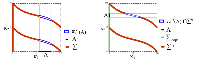
Figure 6.1. (left) A set $A\subset\mathbb{T}$ and its preimage $\boldsymbol{\pi}_{2}^{-1}(A)$. It is visible that $\left|\boldsymbol{\pi}_{2}^{-1}(x)\right|=2$ for every $x\in\mathbb{T}$, except $x=0$. (right) A set $A\subset\mathbb{T}$ and its $\Sigma^{\mathcal{G}}$ preimage $\boldsymbol{\pi}_{1}^{-1}(A)\cap\Sigma^{\mathcal{G}}$. It is visible that $\left|\boldsymbol{\pi}_{1}^{-1}(x)\cap\Sigma^{\mathcal{G}}\right|=1$ for every $x\in\mathbb{T}$, except $x=0,\pi$.

Proof of Lemma 6.7..

Order the edges and compare (4.5) with (4.3). The density of $\mu_{e}$, when restricted to $\Sigma^{\mathrm{reg}}$, is

$$\mathop{\mathrm{\mathstrut d}}\nolimits\!\mu_{e}=\frac{\pi}{(2\pi)^{E}}(-1)^{e-1}\,d\kappa_{1}\wedge d\kappa_{2}\ldots\wedge\widehat{d\kappa_{e}}\ldots\wedge d\kappa_{E}.$$ (6.13)

Given a Borel set $A\subset\mathbb{T}^{E-1}$, integrating (6.13) over $\boldsymbol{\pi}_{e}^{-1}\left(A\right)$ results in

$$\mu_{e}\left(\boldsymbol{\pi}_{e}^{-1}\left(A\right)\right)=\frac{\pi}{(2\pi)^{E}}\int_{A}|\boldsymbol{\pi}_{e}^{-1}({\vec{x}})|\mathop{\mathrm{\mathstrut d}}\nolimits\!{\vec{x}}.$$ (6.14)

The integral on the right-hand-side is well defined since $|\boldsymbol{\pi}_{e}^{-1}({\vec{x}})|=2$ for (Lebesgue) almost every ${\vec{x}}\in\mathbb{T}^{E-1}$ (see the proof of Proposition 3.1 in [25]). Substituting $|\boldsymbol{\pi}_{e}^{-1}({\vec{x}})|=2$ in (6.14) proves the needed equality:

$$\mu_{e}\left(\boldsymbol{\pi}_{e}^{-1}\left(A\right)\right)=\frac{\operatorname{vol}\left(A\right)}{(2\pi)^{E-1}}.$$

To show that the above holds also for the restriction of $\mu_{e}$ to $\Sigma^{\mathcal{G}}$, let us recall the definition of the set $\Sigma_{\textrm{loops}}$ (see Lemma 5.14),

$$\Sigma_{\textrm{loops}}:=\left\{{\vec{\kappa}}\in\mathbb{T}^{E}\,\,:\,\,\exists e\in\mathcal{E}_{\textrm{loops}}\text{ s.t. }\kappa_{e}=0\right\}.$$

Notice that for almost every ${\vec{x}}\in\mathbb{T}^{E-1}$,

$$|\Sigma_{\textrm{loops}}\cap\boldsymbol{\pi}_{e}^{-1}({\vec{x}})|=\begin{cases}1&e\in\mathcal{E}_{\textrm{loops}}\\ 0&e\notin\mathcal{E}_{\textrm{loops}}\end{cases}.$$

We therefore have a constant $c_{e}$ such that $|\boldsymbol{\pi}_{e}^{-1}({\vec{x}})\setminus\Sigma_{\textrm{loops}}|=c_{e}$ for almost every ${\vec{x}}\in\mathbb{T}^{E-1}$. Integrating (6.13) over $\boldsymbol{\pi}_{e}^{-1}\left(A\right)\setminus\Sigma_{\textrm{loops}}$ results in

$$\mu_{e}\left(\boldsymbol{\pi}_{e}^{-1}\left(A\right)\setminus\Sigma_{\textrm{loops}}\right)=\frac{\pi c_{e}}{(2\pi)^{E}}\operatorname{vol}\left(A\right).$$ (6.15)

Lemma 5.14 states that $\Sigma^{\mathcal{G}}$ is equal to $\Sigma\setminus\Sigma_{\textrm{loops}}$ up to a set of measure zero, so

$$\frac{\mu_{e}\left(\boldsymbol{\pi}_{e}^{-1}(A)\cap\Sigma^{\mathcal{G}}\right)}{\mu_{e}(\Sigma^{\mathcal{G}})}=\frac{\mu_{e}\left(\boldsymbol{\pi}_{e}^{-1}(A)\setminus\Sigma_{\textrm{loops}}\right)}{\mu_{e}(\boldsymbol{\pi}_{e}^{-1}(\mathbb{T}^{E-1})\setminus\Sigma_{\textrm{loops}})}=\frac{\operatorname{vol}\left(A\right)}{(2\pi)^{E-1}}.$$ (6.16)

∎

7. Mandarins and stowers - proof of Theorem 3.4

In this section we prove Theorem 3.4 by approximating the nodal surplus distributions of stowers and mandarins in terms of suitable binomial distributions, uniformly in $\beta$. This approximation result is as follows.

Proposition 7.1.

Let $\Gamma$ be either a mandarin or a stower graph with $\beta>1$. Define $N_{\beta}:=\beta-1$ if $\Gamma$ is a stower, and $N_{\beta}:=\beta$ if $\Gamma$ is a mandarin. Let $X_{\beta}$ be a binomial random variable $X_{\beta}\sim\operatorname{Bin}\left(N_{\beta},p=\frac{1}{2}\right)$. Then, for any rationally independent ${\boldsymbol{\ell}}$, the nodal surplus distribution of $\Gamma_{{\boldsymbol{\ell}}}$ satisfies

$$\forall{t\in\mathbb{R}}\qquad P(X_{\beta}\leq t-3)\leq P(\sigma\leq t)\leq P(X_{\beta}\leq t+3).$$ (7.1)

Assuming Proposition 7.1 to be true, we prove Theorem 3.4.

Proof of Theorem 3.4.

Let $\Gamma_{{\boldsymbol{\ell}}}$ be either a stower or a mandarin with rationally independent ${\boldsymbol{\ell}}$ and first Betti number $\beta>1$, and let $\sigma$ be its nodal surplus random variable. We will consider the $\beta\to\infty$ limit without adding $\beta$ superscript to $\Gamma_{{\boldsymbol{\ell}}}$ and $\sigma$, to ease the reading.

Let $X_{\beta}$ and $N_{\beta}$ be as in Proposition 7.1 and observe that $\operatorname{Var}\left(X_{\beta}\right)=N_{\beta}/4$ which grows like $\beta/4$. Denote the normalized random variables,

$$\tilde{X_{\beta}}:=\frac{X_{\beta}-\frac{N_{\beta}}{2}}{\sqrt{\operatorname{Var}\left(X_{\beta}\right)}},\quad\mbox{and}\qquad\tilde{\sigma}:=\frac{\sigma-\frac{\beta}{2}}{\sqrt{\operatorname{Var}\left(X_{\beta}\right)}}.$$

Notice that $\tilde{\sigma}$ is normalized with the variance of $X_{\beta}$. Let $\varepsilon_{\beta}:=\frac{4}{\sqrt{\operatorname{Var}\left(X_{\beta}\right)}}$ and note that $|N_{\beta}-\beta|\leq 1$. We can manipulate (7.1) to show that for any $t\in\mathbb{R}$,

$$P(\tilde{X_{\beta}}\leq t-\varepsilon_{\beta})\leq P(\tilde{\sigma}\leq t)\leq P(\tilde{X_{\beta}}\leq t+\varepsilon_{\beta}).$$ (7.2)

It is known that $\tilde{X_{\beta}}$ converges in distribution to $N(0,1)$ (the standard normal random variable). Now consider (7.2) for a fixed $t\in\mathbb{R}$ and let $\beta\rightarrow\infty$. Since $\varepsilon_{\beta}\rightarrow 0$ and $N(0,1)$ has continuous distribution, we establish that $\tilde{\sigma}$ also converges in distribution to $N(0,1)$. In particular,

$$1=\lim_{\beta\rightarrow\infty}\operatorname{Var}\left(\tilde{\sigma}\right)=\lim_{\beta\rightarrow\infty}\frac{\operatorname{Var}\left(\sigma\right)}{\operatorname{Var}\left(X_{\beta}\right)},$$

which proves that $\operatorname{Var}\left(\sigma\right)$ grows like $\beta/4$ and that the properly normalized random variable, $\frac{\sigma-\frac{\beta}{2}}{\sqrt{\operatorname{Var}\left(\sigma\right)}}=\sqrt{\frac{\operatorname{Var}\left(\sigma\right)}{\operatorname{Var}\left(X_{\beta}\right)}}\tilde{\sigma}$, converges in distribution to $N(0,1)$ as needed. ∎

We now return to the proof of Proposition 7.1. A crucial part of the proof is that for mandarins and stowers, the function $\boldsymbol{\sigma}$ can be expressed explicitly, as seen in Lemmas A.5 and A.9 in [4]. We restate the needed results from Lemmas A.5 and A.9 as follows:

Lemma 7.2.

[4] Let $\Gamma$ be a mandarin or a stower. There is a negligible set $B$ with $\dim{(B)}\leq E-2$, such that

1. If $\Gamma$ is a stower, then for any ${\vec{\kappa}}\in\Sigma^{\mathcal{G}}\setminus{B}$

   $$\boldsymbol{\sigma}({\vec{\kappa}})=\Big{|}\left\{e\in\mathcal{E}_{\textrm{loops}}\,\,:\,\,\pi<\kappa_{e}<2\pi\right\}\Big{|}.$$ (7.3)

2. If $\Gamma$ is a mandarin graph, then for any ${\vec{\kappa}}\in\Sigma^{\mathcal{G}}\setminus{B}$, either

   $$\boldsymbol{\sigma}({\vec{\kappa}})=\Big{|}\left\{e\in\mathcal{E}\,\,:\,\,\pi<\kappa_{e}<2\pi\right\}\Big{|}-C({\vec{\kappa}}),$$ (7.4)

   or,

   $$E-\boldsymbol{\sigma}({\vec{\kappa}})=\Big{|}\left\{e\in\mathcal{E}\,\,:\,\,\pi<\kappa_{e}<2\pi\right\}\Big{|}-C({\vec{\kappa}}),$$ (7.5)

   with some bounded error function $C:\Sigma^{\mathcal{G}}\to\{-1,0,1\}$.

Remark 7.3.

The set $\Sigma^{\text{gen}}$ defined in [4] is a subset of $\Sigma^{\mathcal{G}}$, reflecting a more restrictive definition of generic eigenfunctions. The set $B$ in the above lemma is the difference $\Sigma^{\mathcal{G}}\setminus\Sigma^{\text{gen}}$, which has $\dim\left(\Sigma^{\mathcal{G}}\setminus\Sigma^{\text{gen}}\right)\leq E-2$ as seen in [2, 3].

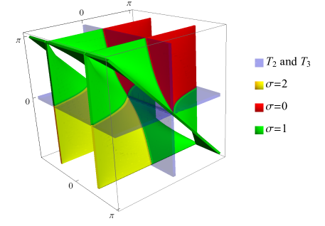
(a)

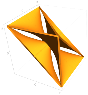
(b)

Figure 7.1. On the left, the secular manifold $\Sigma$ of a stower with one tail $e_{1}$ and two loops $e_{2}$ and $e_{3}$, presented in $(-\pi,\pi)^{3}$. The loops related part is the union of two sub-tori, $\Sigma_{\textrm{loops}}=T_{2}\cup T_{3}$, with $T_{j}:=\left\{{\vec{\kappa}}\in\mathbb{T}^{3}\,\,:\,\,\kappa_{j}=0\right\}$, presented in low opacity. The rest is colored according to the values of $\boldsymbol{\sigma}$. On the right, the secular manifold $\Sigma$ of a mandarin with three edges. In this case $\boldsymbol{\sigma}\equiv 1$.

Examples of $\Sigma$ and the function $\boldsymbol{\sigma}$ are shown in figure 7.1. The next step towards proving Proposition 7.1 is introducing an auxiliary function $\boldsymbol{\xi}$ which approximates $\boldsymbol{\sigma}$.

Definition 7.4.

Given a graph $\Gamma$, we choose $e_{1}\in\mathcal{E}$ and $\widetilde{\mathcal{E}}\subset\mathcal{E}$ as follows.

1. If $\Gamma$ is a stower (which is not a star) let $e_{1}$ be a loop, and let $\widetilde{\mathcal{E}}:=\mathcal{E}_{\textrm{loops}}\setminus e_{1}$.

2. If $\Gamma$ is a mandarin, let $e_{1}$ be any edge and let $\widetilde{\mathcal{E}}:=\mathcal{E}\setminus e_{1}$.

In both cases, $|\widetilde{\mathcal{E}}|=N_{\beta}$. Define the function $\boldsymbol{\xi}:\Sigma\to\{0,1\ldots,N_{\beta}\}$ by

$$\boldsymbol{\xi}({\vec{\kappa}}):=\Big{|}\left\{e\in\widetilde{\mathcal{E}}\,\,:\,\,\pi<\kappa_{e}<2\pi\right\}\Big{|}.$$ (7.6)

For every edge $e$ we define a random variable $\xi_{e}$, taking values in $\{0,1,\ldots,N_{\beta}\}$, with probability

$$P(\xi_{e}=j)=\frac{\mu_{e}\left(\Sigma^{\mathcal{G}}\cap\boldsymbol{\xi}^{-1}\left(j\right)\right)}{\mu_{e}\left(\Sigma^{\mathcal{G}}\right)}.$$ (7.7)

Lemma 7.5.

If $e\notin\widetilde{\mathcal{E}}$ then $\xi_{e}\sim\mathop{Bin}\left(N_{\beta},p=\frac{1}{2}\right)$, namely

$$P(\xi_{e}=j)=\binom{N_{\beta}}{j}2^{-N_{\beta}},\qquad j=0,1,2,\ldots,N_{\beta}.$$ (7.8)

Proof.

Consider the canonical projection $\boldsymbol{\pi}_{e}$ (see Lemma 6.7) such that the entries of ${\vec{x}}=\boldsymbol{\pi}_{e}^{-1}({\vec{\kappa}})$ are $x_{e^{\prime}}=\kappa_{e^{\prime}}$ for $e^{\prime}\in\mathcal{E}\setminus{e}$. Since $e\notin\tilde{\mathcal{E}}$, the level sets of $\boldsymbol{\xi}$ are given by

$$\boldsymbol{\xi}^{-1}(j)=\left\{{\vec{\kappa}}\in\Sigma\,\,:\,\,\left|\left\{e^{\prime}\in\tilde{\mathcal{E}}\,\,:\,\,\pi<\kappa_{e^{\prime}}<2\pi\right\}\right|=j\right\}=\boldsymbol{\pi}_{e}^{-1}\left(A_{j}\right),$$

with

$$A_{j}:=\left\{{\vec{x}}\in\mathbb{T}^{E-1}\,\,:\,\,\left|\left\{e^{\prime}\in\tilde{\mathcal{E}}\,\,:\,\,\pi<{\vec{x}}_{e^{\prime}}<2\pi\right\}\right|=j\right\}.$$

Applying Lemma 6.7 gives

$$P(\xi_{e}=j)= \frac{\mu_{e}\left(\Sigma^{\mathcal{G}}\cap\boldsymbol{\xi}^{-1}\left(j\right)\right)}{\mu_{e}\left(\Sigma^{\mathcal{G}}\right)}$$

$$= \frac{\mu_{e}\left(\Sigma^{\mathcal{G}}\cap\boldsymbol{\pi}_{e}^{-1}\left(A_{j}\right)\right)}{\mu_{e}\left(\Sigma^{\mathcal{G}}\right)}$$

$$= \frac{\operatorname{vol}\left(A_{j}\right)}{(2\pi)^{E-1}}.$$

It is a simple observation that

$$\frac{\operatorname{vol}\left(A_{j}\right)}{(2\pi)^{E-1}}=\binom{|\tilde{\mathcal{E}}|}{j}2^{-|\tilde{\mathcal{E}}|}=\binom{N_{\beta}}{j}2^{-N_{\beta}},$$

which proves the lemma. ∎

The proof of the proposition follows.

Proof of Proposition 7.1.

Recall the random variables $\omega_{e}$, taking values in $\{0,1,\ldots,\beta\}$, with probability (see (6.4)),

$$P(\omega_{e}=j):=W_{e,j}=\frac{\mu_{e}\left(\Sigma^{\mathcal{G}}\cap\boldsymbol{\sigma}^{-1}(j)\right)}{\mu_{e}\left(\Sigma^{\mathcal{G}}\right)}.$$ (7.9)

By (6.5), the nodal surplus distribution of $\Gamma_{{\boldsymbol{\ell}}}$, for ${\boldsymbol{\ell}}$ rationally independent, satisfies

$$\forall t\in\mathbb{R},\qquad P(\sigma\leq t)=\frac{1}{\sum_{e\in\mathcal{E}}\ell_{e}c_{e}}\sum_{e\in\mathcal{E}}\ell_{e}c_{e}P(\omega_{e}\leq t),$$ (7.10)

and so to prove the proposition, we will show that for every edge $e\in\mathcal{E}$,

$$\forall t\in\mathbb{R},\qquad P(X_{\beta}<t-3)\leq P(\omega_{e}<t)\leq P(X_{\beta}<t+3).$$ (7.11)

In fact, if $G_{\Gamma}$ is the symmetry group of $\Gamma$, then according to Theorem 6.4 it is enough to prove (7.11) for one representative edge per equivalence class in $\mathcal{E}/G_{\Gamma}$. Recalling the choice of $e_{1}$ in Definition 7.4, we have the following.

1. If $\Gamma$ is a mandarin or a flower, then $\mathcal{E}/G_{\Gamma}=\{[e_{1}]\}$ and so it is enough to show that (7.11) holds for $\omega_{e_{1}}$.

2. If $\Gamma$ is a stower which is not a flower or a star, then $\mathcal{E}/G_{\Gamma}=\{[e_{1}],[e_{2}]\}$ where $e_{2}\notin\mathcal{E}_{\textrm{loops}}$, and so it is enough to prove (7.11) for $\omega_{e_{1}}$ and $\omega_{e_{2}}$.

We proceed by proving the proposition for stowers. Assume that $\Gamma$ is a stower (possibly a flower). Recall that $\widetilde{\mathcal{E}}:=\mathcal{E}_{\textrm{loops}}\setminus e_{1}$ and compare (7.6) with (7.3), to get

$$\left|\boldsymbol{\sigma}({\vec{\kappa}})-\boldsymbol{\xi}({\vec{\kappa}})\right|\leq 1,$$ (7.12)

for every ${\vec{\kappa}}\in\Sigma^{\mathcal{G}}\setminus{B}$, for some $B$ of measure zero. If we neglect $B$, this gives

$$\Sigma^{\mathcal{G}}\cap\boldsymbol{\xi}^{-1}\left((-\infty,t-1]\right)~{}\subset~{}\Sigma^{\mathcal{G}}\cap\boldsymbol{\sigma}^{-1}\left((-\infty,t]\right)~{}\subset~{}\Sigma^{\mathcal{G}}\cap\boldsymbol{\xi}^{-1}\left((-\infty,t+1]\right).$$

Given any $e\in\mathcal{E}$, compare $\omega_{e}$ and $\xi_{e}$ (see (7.9) and (7.7)) to conclude that

$$\forall{t\in\mathbb{R}}\qquad P(\xi_{e}\leq t-1)\leq P(\omega_{e}\leq t)\leq P(\xi_{e}\leq t+1).$$ (7.13)

In particular, if $e\notin\widetilde{\mathcal{E}}$, then $\xi_{e}$ has the same probability distribution as $X_{\beta}$ by Lemma 7.5,

$$\forall t\in\mathbb{R},\qquad P(X_{\beta}\leq t-1)\leq P(\omega_{e}\leq t)\leq P(X_{\beta}\leq t+1).$$ (7.14)

This proves Proposition 7.1 for stowers, as $e_{1}\notin\widetilde{\mathcal{E}}$ and if $e_{2}\notin\mathcal{E}_{\textrm{loops}}$ then also $e_{2}\notin\widetilde{\mathcal{E}}$.

We proceed with proving Proposition 7.1 for mandarins. Let $\Gamma$ be a mandarin graph, choose $e_{1}$ to be any edge and define $\widetilde{\mathcal{E}}$ and $\xi$ correspondingly, as in Definition 7.4. As before, Lemma 7.5 ensures that $\xi_{e_{1}}$ is binomial like $X_{\beta}$, and so it is left to prove

$$\forall{t\in\mathbb{R}}\qquad P(\xi_{e_{1}}\leq t-3)\leq P(\omega_{e_{1}}\leq t)\leq P(\xi_{e_{1}}\leq t+3).$$ (7.15)

Notice that both $\xi_{e_{1}}$ and $\omega_{e_{1}}$ are symmetric around $\frac{\beta}{2}$: $\xi_{e_{1}}$ since it is binomial with $p=\frac{1}{2}$ and $N_{\beta}=\beta$, and $\omega_{e_{1}}$ due to (6.7). Under such symmetry, (7.15) is equivalent to

$$P\left(\left|\xi_{e_{1}}-\frac{\beta}{2}\right|\leq t-3\right)\leq P\left(\left|\omega_{e_{1}}-\frac{\beta}{2}\right|\leq t\right)\leq P\left(\left|\xi_{e_{1}}-\frac{\beta}{2}\right|\leq t+3\right),$$ (7.16)

for all $t\geq 0$. Let us now prove (7.16).

According to Lemma 7.2, given any ${\vec{\kappa}}\in\Sigma^{\mathcal{G}}\setminus B$, one of the following is true:

1. Equation (7.4) holds. Comparing (7.4) and (7.6), using $|C|\leq 1$ and $\widetilde{\mathcal{E}}:=\mathcal{E}\setminus{e_{1}}$ gives $\left|\boldsymbol{\xi}({\vec{\kappa}})-\boldsymbol{\sigma}({\vec{\kappa}})\right|\leq 2$. We may write it as

   $$\left|\left(\boldsymbol{\xi}({\vec{\kappa}})-\frac{\beta}{2}\right)-\left(\boldsymbol{\sigma}({\vec{\kappa}})-\frac{\beta}{2}\right)\right|\leq 2,$$ (7.17)

2. Equation (7.5) holds, and a similar argument gives $\left|\boldsymbol{\xi}({\vec{\kappa}})-(E-\boldsymbol{\sigma}({\vec{\kappa}}))\right|\leq 2$. Recall that for mandarins $E=\beta+1$, so $\left|\boldsymbol{\xi}({\vec{\kappa}})+(\boldsymbol{\sigma}({\vec{\kappa}})-\beta)\right|\leq 3$. We may write it as

   $$\left|\left(\boldsymbol{\xi}({\vec{\kappa}})-\frac{\beta}{2}\right)+\left(\boldsymbol{\sigma}({\vec{\kappa}})-\frac{\beta}{2}\right)\right|\leq 3.$$ (7.18)

In both cases

$$-3\leq\left|\boldsymbol{\xi}({\vec{\kappa}})-\frac{\beta}{2}\right|-\left|\boldsymbol{\sigma}({\vec{\kappa}})-\frac{\beta}{2}\right|\leq 3.$$ (7.19)

As this holds for all ${\vec{\kappa}}\in\Sigma^{\mathcal{G}}\setminus{B}$, we conclude that (7.16) is true using the same arguments as before. This finishes the proof of the proposition. ∎

Acknowledgments

We thank the referees for valuable comments. We thank Ronen Eldan for interesting discussions. The authors were supported by the Binational Science Foundation Grant (Grant No. 2016281). RB and LA were also supported by ISF (Grant No. 844/19). LA was also supported by the Ambrose Monell Foundation and the Institute for Advanced Study. GB was also supported by the National Science Foundation (DMS-1815075).

Appendix A Continuous eigenvalues of Unitary matrices

In sections 4 and 5, we consider an analytic family of unitary matrices and their eigenvalues. In this appendix we deal with the question of whether the eigenvalues of a continuous family of unitary matrices can be written as continuous functions. The general setting is as follows: Let $\textbf{U}(N)$ be the unitary group of $N\times N$ matrices and a consider a continuous family of matrices $U_{x}\in\textbf{U}(N),~{}~{}x\in M$, for some (finite dimensional) manifold $M$ with or without boundary. We say that the family is continuous if the map $x\mapsto U_{x}$ is a continuous map from $M$ to $\textbf{U}(n)$.

Definition A.1.

We say that the family $U_{x}$ for $x\in M$ has a continuous counterclockwise ordering (CC ordering) of eigenvalues if there exist $N$ continuous functions (eigenvalues)

$$\lambda_{n}:M\to S^{1},\qquad n=1,2,\ldots,N$$

and $N$ continuous functions (the phase gaps),

$$a_{n}:M\to[0,2\pi],\qquad n=1,\ldots N,$$

such that

1. The eigenvalues of $U_{x}$ at every $x\in M$ are $\{\lambda_{n}(x)\}_{n=1}^{N}$ with multiplicity.

2. At every $x\in M$,

   $$a_{1}+a_{2}+\ldots+a_{N} =2\pi$$

   $$\lambda_{2}=\lambda_{1}e^{ia_{1}},\quad\lambda_{3}=\lambda_{2}e^{ia_{2}}, \ \ldots,\ \lambda_{1}=\lambda_{N}e^{ia_{N}}.$$

Remark A.2.

Notice that if $\{(\lambda_{1},\lambda_{2},\ldots,\lambda_{N}),(a_{1},a_{2},\ldots,a_{N})\}$ is a CC ordering, then a cyclic permutation such as $\{(\lambda_{2},\ldots,\lambda_{N},\lambda_{1}),(a_{2},\ldots,a_{N},a_{1})\}$ is also a CC ordering. The inclusion of both eigenvalues and the phase gaps ensures that a CC ordering (if exists) is unique up to such cyclic permutation. Moreover, these cyclic permutations are distinct (as ordered tuples) at every point $x\in M$, including the two cases where either all eigenvalues are equal, or all phase gaps are equal.

Remark A.3.

Locally, the eigenvalues can always be ordered in such a fashion, but the question is whether the ordering extends globally. The local argument is as follows. Given $x\in M$ choose $t\in\mathbb{R}$ such that $e^{it}$ is not an eigenvalue of $U_{x}$. The set of eigenvalues depends continuously on the matrix entries, so there exists a neighborhood $\Omega_{x}$ of $x$ such that $e^{it}$ is not an eigenvalue of any $U_{x^{\prime}}$ for any $x^{\prime}\in\Omega_{x}$. Then, the eigenvalues of $U_{x^{\prime}}$ with $x^{\prime}\in\Omega_{x}$ can be written as $\lambda_{n}(x^{\prime})=e^{i\theta_{n}(x^{\prime})}$, where $\theta_{n}(x^{\prime})\in(t,t+2\pi)$ are ordered increasingly and are continuous in $x^{\prime}\in\Omega_{x}$. Now the claim follows by setting $a_{N}=\theta_{1}+2\pi-\theta_{N}$ and $a_{n}=\theta_{n+1}-\theta_{n+1}$ for $n<N$.

Given $\gamma$, a closed path in $M$, let $[\gamma]$ denote its homotopy equivalence class. For a continuous function $f:M\to S^{1}$, denote its winding number along $\gamma$ by $\operatorname{\textbf{w}}([\gamma],f)\in\mathbb{Z}$. The induced homomorphism $f_{*}:\pi_{1}(M)\to\mathbb{Z}$ is defined by

$$f_{*}([\gamma]):=\operatorname{\textbf{w}}([\gamma],f).$$

Proposition A.4.

Given a continuous family of unitary matrices, $U_{x}\in\textbf{U}(N),~{}x\in M$, the function $x\mapsto\det(U_{x})$ is continuous from $M$ to $S^{1}$. There is a CC ordering of the eigenvalues if and only if

$$\det(U_{x})_{*}\equiv 0~{}~{}\mod N.$$ (A.1)

In particular,

1. If $M$ is simply connected, then there exist a continuous counterclockwise ordering of the eigenvalues.

2. Let $M=\mathbb{T}^{E},~{}~{}N=2E,~{}~{}E>1$ and $S\in\textbf{U}(2E)$, as in Definition 3.6. If the family of unitary matrices has the form

   $$U_{{\vec{\kappa}}}:=\textrm{diag}(e^{i\kappa_{1}},e^{i\kappa_{2}},\ldots,e^{i\kappa_{N}},e^{i\kappa_{1}},e^{i\kappa_{2}},\ldots,e^{i\kappa_{N}})S\in\textbf{U}(2E),\quad\mbox{with}\quad{\vec{\kappa}}\in\mathbb{T}^{E},$$

   then there is no CC ordering of the eigenvalues.

Proof of Proposotion A.4.

The proof consists of three parts. Part I, where we show that having a CC ordering leads to (A.1). Part II, where we assume that (A.1) holds, and construct the needed CC ordering. Part III, where we prove (1) and (2). For the ease of reading, we first prove Part III, assuming Part I and Part II. That is, we need to show that in case (1) (A.1) holds while in case (2) (A.1) fails.

Part III (assuming Part I and Part II) -

1. If $M$ is simply connected then $\pi_{1}(M)$ is trivial and therefore any homomorphism from it is trivial, namely $\det(U_{x})_{*}\equiv 0$.

2. Consider the family discussed above. Namely, $N=2E$ and $M=\mathbb{T}^{E}$ and

   $$U_{{\vec{\kappa}}}:=\textrm{diag}(e^{i\kappa_{1}},e^{i\kappa_{2}},\ldots,e^{i\kappa_{N}},e^{i\kappa_{1}},e^{i\kappa_{2}},\ldots,e^{i\kappa_{N}})S.$$

   Consider the closed path $\gamma$ in $\mathbb{T}^{E}$, defined by $\gamma(t)=(t,0,0,\ldots,0)$ for $t\in\mathbb{R}/2\pi\mathbb{Z}$. Then $\det(U_{\gamma(t)})=e^{2it}\det(S)$ and so the winding number of $\det(U_{{\vec{\kappa}}})$ along $\gamma$ is $2$. If $E>1$ then $2$ is not a multiple of $2E$ and therefore (A.1) fails.

Part I - Let $U_{x}$ for $x\in M$ be a continuous family of unitary matrices and assume that there exist a continuous counterclockwise ordering of their eigenvalues. Consider the $\lambda_{n}$’s and $a_{n}$’s described in Definition A.1. Notice that $\operatorname{\textbf{w}}([\gamma],e^{ia_{n}})=0$ for any continuous $a_{n}:M\to[0,2\pi]$ and any $[\gamma]$. In other words, the induced homomorhpism is trivial, $(e^{ia_{n}})_{*}\equiv 0$. Since the winding of a product of functions is the sum of the winding of the functions, then for any $n\geq 2$

$$(\lambda_{n})_{*}=(e^{ia_{n-1}}\lambda_{n-1})_{*}=(\lambda_{n-1})_{*}+(e^{ia_{n-1}})_{*}=(\lambda_{n-1})_{*}=\ldots=(\lambda_{1})_{*}.$$

Therefore, using $\det(U_{x})=\prod_{n=1}^{N}\lambda_{n}$, we get

$$\det(U_{x})_{*}=\sum_{n=1}^{N}(\lambda_{n})_{*}=N(\lambda_{1})_{*}$$

which proves Part II.

Part II - Let $U_{x}$ for $x\in M$ be a continuous family of unitary matrices and assume that

$$\det(U_{x})_{*}\equiv 0~{}~{}\mod N.$$

To construct the CC ordering of the eigenvalues we use three steps. The first step is showing that any path $\gamma:[0,1]\to M$ admits a unique CC ordering that depends only on the initial ordering of the eigenvalues at $\gamma(0)$. The second step is to show that the ordering at the final point $\gamma(1)$ actually depends only on the initial ordering at $\gamma(0)$ and not on the path $\gamma$. The third step is then to fix some initial point $x_{0}\in M$ with initial ordering, and number the eigenvalues at any other point $x\in M$ by a path going from $x_{0}$ to $x$. Then, the previous steps ensure that this is indeed a CC ordering.

Constructing CC ordering along a path - According to Remark A.3, any $x\in M$ has a neighborhood $\Omega_{x}$ for which there is a CC ordering of the eigenvalues. Assume that two such neighborhoods $\Omega_{x}$ and $\Omega_{x^{\prime}}$ intersect and that each neighborhood has its CC ordering. If both CC orderings agree on $\Omega_{x}\cap\Omega_{x^{\prime}}$ then by definition we have a CC ordering for the union $\Omega_{x}\cup\Omega_{x^{\prime}}$. Otherwise, they can only differ by a cyclic permutation on $\Omega_{x}\cap\Omega_{x^{\prime}}$, according to Remark A.2, in which case we may cyclically permute the CC ordering at $\Omega_{x^{\prime}}$ and get a CC ordering on $\Omega_{x}\cup\Omega_{x^{\prime}}$. Given a path $\gamma:[0,1]\to M$, we can cover it by finitely many such neighborhoods, each with its CC ordering. Denote the neighborhoods along $\gamma$ by $\Omega_{j}$ for $j=1,2,\ldots,J$, ordered increasingly. Applying the above procedure to every pair of $\Omega_{j}$ and $\Omega_{j+1}$, permuting the CC ordering of $\Omega_{j+1}$ if needed, we get a CC ordering along $\gamma$. It is now clear that the ordering of the eigenvalues at the final point $\gamma(1)$ is uniquely determined by the path $\gamma$ and the ordering at the initial point $\gamma(0)$.

CC ordering along a closed path - Consider the case that $\gamma$ is closed, $\gamma(1)=\gamma(0)$. A priori, the initial and final ordering may differ by a cyclic permutation. We now show that the assumption of (A.1), namely $\det(U_{x})_{*}\equiv 0~{}~{}\mod N$, implies that the initial ordering is equal to the final ordering. Let

$$\lambda_{n}:[0,1]\to S^{1},\qquad a_{n}:[0,1]\to[0,2\pi],\qquad n=1,2,\ldots,N,$$

be the CC ordering of the eigenvalues of $U_{\gamma(t)}$ for $t\in[0,1]$. Assume by contradiction that the final ordering differ from the initial ordering. Then, for some $1\leq d\leq N-1$,

$$\lambda_{1}(1)=\lambda_{1+d}(0)$$

$$\qquad\vdots$$

$$\lambda_{N-d}(1)=\lambda_{N}(0)$$

$$\lambda_{N-d+1}(1)=\lambda_{1}(0)$$

$$\qquad\vdots$$

$$\lambda_{N}(1)=\lambda_{d}(0).$$

By the Lifting Theorem, there is a continuous function $\theta_{1}:[0,1]\to\mathbb{R}$ such that $\lambda_{1}=e^{i\theta_{1}}$. Define inductively $\theta_{n+1}:=\theta_{n}+a_{n}$, so that each $\theta_{n}:[0,1]\to\mathbb{R}$ is continuous and satisfies $\lambda_{n}=e^{i\theta_{n}}$. Due to the properties of the $a_{n}$ functions, the $\theta_{n}$ functions are ordered in a $2\pi$ interval for every $t\in[0,1]$,

$$\theta_{1}\leq\theta_{2}\leq\ldots\leq\theta_{N}=\theta_{1}+2\pi-a_{N}\leq\theta_{1}+2\pi.$$

We may deduce that

$$\theta_{1}(1)=\theta_{1+d}(0)+2\pi m$$

$$\qquad\vdots$$

$$\theta_{N-d}(1)=\theta_{N}(0)+2\pi m$$

$$\theta_{N-d+1}(1)=\theta_{1}(0)+2\pi(m+1)$$

$$\qquad\vdots$$

$$\theta_{N}(1)=\theta_{d}(0)+2\pi(m+1)$$

for some integer $m\in\mathbb{Z}$. Since $\det(U_{\gamma(t)})=e^{i\sum\theta_{n}(t)}$, then the winding number of $\det(U_{x})$ along $\gamma$ is equal to

$$\operatorname{\textbf{w}}(\det(U_{x}),\gamma) =\frac{1}{2\pi}\left(\sum_{n=1}^{N}\theta_{n}(1)-\sum_{n=1}^{N}\theta_{n}(0)\right)$$

$$=mN+d.$$

Since $1\leq d\leq N-1$, this is a contradiction to (A.1).

Path independence of the ordering - Consider an initial point $x_{0}\in M$ with a fixed ordering and let $x\in M$ be another point. Assume by contradiction that there are two paths $\gamma$ and $\gamma^{\prime}$ from $x_{0}$ to $x$ whose CC orderings do not agree at the final point $x$. Let $\phi$ be the closed path obtained by concatenation of $\gamma^{\prime}$ in reverse with $\gamma$. Namely, starting from $\phi(0)=x$, going along $\gamma^{\prime}$ backwards to $x_{0}$ (where both the CC ordering agree) and then along $\gamma$ back to $\phi(1)=x$. The CC ordering along $\varphi$ is then defined by that of $\gamma^{\prime}$ (reversing is obtained by re-parameterization $t\mapsto 1-t$) and that of $\gamma$, which agree at the concatenation point $x_{0}$, and leads to the disagreement between the initial ordering at $x=\phi(0)$ and the final at $x=\varphi(1)$. Contradiction. Hence, the ordering that $x$ inherit from $x_{0}$ is independent of the path between them.

Constructing CC ordering on $M$ - Fix an arbitrary initial point $x_{0}$ and an initial ordering. Then any $x\in M$ inherits a unique ordering, $\{(\lambda_{1}(x),\ldots,\lambda_{N}(x)),(a_{1}(x),\ldots,a_{N}(x))\}$ which satisfies (1) and (2) of Definition A.1. As this ordering agree with the (unique) CC ordering along any path going from $x_{0}$ to $x$, then $\{(\lambda_{1}(x),\ldots,\lambda_{N}(x)),(a_{1}(x),\ldots,a_{N}(x))\}$ must be continuous along any path in $M$, and hence continuous in $M$. ∎

Appendix B Proof of Lemma 3.9.

Let us restate the lemma. Recall that given a random variable $X$ we defined $N(X)$ as a normal (Gaussian) random variable with mean $\mathbb{E}(X)$ and variance $\operatorname{Var}(X)$ (assuming these exist). Consider the distance between two random variables $X,Y$ to be

$$d_{KS}(X,Y):=\sup_{t\in\mathbb{R}}\left|P(X\leq t)-P(Y\leq t)\right|,$$ (B.1)

as defined in (3.3).

Remark B.1.

Notice that $d_{KS}(X,Y)$ is a distance between the cumulative probability functions and is independent of the probability spaces on which $X$ and $Y$ are defined. The same is true for $\operatorname{Var}(X)$ and $\operatorname{Var}(Y)$. For this reason we do not specify at any point what are the probability spaces of these random variables.

Lemma 3.9 can be written as follows.

Lemma B.2.

Fix positive integers $\beta,E\in\mathbb{N}$, and consider a set of random variables $\{\omega_{e}\}_{e=1}^{E}$, all taking values in $\{0,1,\ldots,\beta\}$ symmetrically, namely

$$P(\omega_{e}=s)=P(\omega_{e}=\beta-s),\qquad s=0,1,\ldots,\beta,$$

for every $e=1,2,\ldots,E$. Let $\sigma$ be another random variable that takes values in $\{0,1,\ldots,\beta\}$ symmetrically, and satisfies

$$P(\sigma=s)=\frac{1}{L}\sum_{e\in\mathcal{E}}\ell_{e}P(\omega_{e}=s),\qquad s=0,1,\ldots,\beta,$$ (B.2)

for some ${\boldsymbol{\ell}}\in\mathbb{R}_{+}^{E}$ with $L=\sum_{e\in\mathcal{E}}\ell_{e}$. Then,

1. $d_{KS}(\sigma,N(\sigma))$ is bounded by

   $$d_{KS}(\sigma,N(\sigma))\leq\max_{e\in\mathcal{E}}d_{KS}(\omega_{e},N(\omega_{e}))+\varepsilon,$$ (B.3)

   where $\varepsilon:=\sqrt{\frac{\max_{e\in\mathcal{E}}\operatorname{Var}(\omega_{e})}{\min_{e\in\mathcal{E}}\operatorname{Var}(\omega_{e})}}-1$.

2. The variances satisfy

   $$\min_{e\in\mathcal{E}}\operatorname{Var}\left(\omega_{e}\right)\leq\operatorname{Var}(\sigma)\leq\max_{e\in\mathcal{E}}\operatorname{Var}\left(\omega_{e}\right).$$ (B.4)

Proof.

First, due to the symmetry, every $\omega_{e}$ has mean $\frac{\beta}{2}$ and so does $\sigma$. Together with (B.2), this leads to $\operatorname{Var}{(\sigma)}=\frac{1}{L}\sum_{e\in\mathcal{E}}\ell_{e}\operatorname{Var}{(\omega_{e})}$ from which (B.4) follows. We proceed with proving (B.3). Using (B.2), we may write $d_{KS}(\sigma,N(\sigma))$ as

$$d_{KS}(\sigma,N(\sigma))= \sup_{t\in\mathbb{R}}|\frac{1}{L}\sum_{e\in\mathcal{E}}\ell_{e}P(\omega_{e}\leq t)-P(N(\sigma)\leq t)|$$

$$\leq \sup_{t\in\mathbb{R}}\frac{1}{L}\sum_{e\in\mathcal{E}}\ell_{e}|P(\omega_{e}\leq t)-P(N(\sigma)\leq t)|$$

$$\leq \frac{1}{L}\sum_{e\in\mathcal{E}}\ell_{e}d_{KS}(\omega_{e},N(\sigma))$$

$$\leq \max_{e\in\mathcal{E}}d_{KS}(\omega_{e},N(\sigma))$$

$$\leq \max_{e\in\mathcal{E}}d_{KS}(\omega_{e},N(\omega_{e}))+\max_{e\in\mathcal{E}}d_{KS}(N(\omega_{e}),N(\sigma)).$$

We are left with showing that $\max_{e\in\mathcal{E}}d_{KS}(N(\omega_{e}),N(\sigma))\leq\varepsilon:=\sqrt{\frac{\max_{e\in\mathcal{E}}\operatorname{Var}{\omega_{e}}}{\min_{e\in\mathcal{E}}\operatorname{Var}{\omega_{e}}}}-1$. To do so, recall that both $N(\omega_{e})$ and $N(\sigma)$ are normal with the same mean, $\frac{\beta}{2}$, and possibly different variances. Let $s_{1}^{2}$ be the smaller variance and $s_{2}^{2}$ be the larger variance, so that

$$d_{KS}(N(\omega_{e}),N(\sigma))= \sup_{t\in\mathbb{R}}|\int_{-\infty}^{t}\frac{e^{-\frac{1}{2}(\frac{x-\frac{\beta}{2}}{s_{1}})^{2}}}{\sqrt{2\pi}}\frac{\mathop{\mathrm{\mathstrut d}}\nolimits\!x}{s_{1}}-\int_{-\infty}^{t}\frac{e^{-\frac{1}{2}(\frac{x-\frac{\beta}{2}}{s_{2}})^{2}}}{\sqrt{2\pi}}\frac{\mathop{\mathrm{\mathstrut d}}\nolimits\!x}{s_{2}}|$$

$$= \frac{1}{\sqrt{2\pi}}\sup_{t\in\mathbb{R}}|\int_{-\infty}^{\frac{t}{s_{1}}}e^{-\frac{x^{2}}{2}}\mathop{\mathrm{\mathstrut d}}\nolimits\!x-\int_{-\infty}^{\frac{t}{s_{2}}}e^{-\frac{x^{2}}{2}}\mathop{\mathrm{\mathstrut d}}\nolimits\!x|$$

$$= \frac{1}{\sqrt{2\pi}}\sup_{t\geq 0}\int_{\frac{t}{s_{2}}}^{\frac{t}{s_{1}}}e^{-\frac{x^{2}}{2}}\mathop{\mathrm{\mathstrut d}}\nolimits\!x$$

$$\leq \frac{1}{\sqrt{2\pi}}\sup_{t\geq 0}e^{-\frac{(\frac{t}{s_{2}})^{2}}{2}}(\frac{t}{s_{1}}-\frac{t}{s_{2}})$$

$$= \frac{e^{-\frac{1}{2}}}{\sqrt{2\pi}}(\frac{s_{2}}{s_{1}}-1)$$

$$\leq \frac{s_{2}}{s_{1}}-1.$$

As the variance inequality (B.4) gives

$$\min_{e\in\mathcal{E}}\operatorname{Var}{(\omega_{e})}\leq s_{1}^{2}\leq s_{2}^{2}\leq\max_{e\in\mathcal{E}}\operatorname{Var}{(\omega_{e})},$$

we may deduce that $\frac{s_{2}}{s_{1}}-1\leq\sqrt{\frac{\max_{e\in\mathcal{E}}\operatorname{Var}{\omega_{e}}}{\min_{e\in\mathcal{E}}\operatorname{Var}{\omega_{e}}}}-1=\varepsilon$. This finishes the proof.

∎

Appendix C Images from the numerical experiments

The experiment described in Subsection 3.4.1 considered the following graphs:

1. Complete graphs of $n$ vertices for $n\in\{5,\ldots 12\}$.

2. Periodic ladder graphs of $n$ steps for $n\in\{6,10,14,18,22\}$.

3. Periodic square lattices of $n^{2}$ vertices for $n\in\{4,5,6,7\}$.

4. Random $5$-regular graphs of $n$ vertices for $n\in\{12,14,16,18,20\}$.

5. Random Erdős-Rényi graphs with $n$ vertices and $p=0.75$, for $n\in\{9,10,11,12\}$.

We emphasize again that the randomly chosen graphs are not an average over random samples of graphs but rather one sample per type (as we discuss in Remark 3.10). The figures in Subsection 3.4.2 provide the needed evidence for convergence to Gaussian with variance that grows linear in $\beta$. We provide complement figures in which the convergence of the distributions can be seen visually. Each figure shows the convergence for one family of graphs. For every graph in such a family we present the distribution of the $\omega_{e}$ which maximize $d_{KS}\left(\omega_{e},N(\omega_{e})\right)$ (namely the “worst” candidate). The different graphs in each family are labeled by their first Betti number $\beta$ (for the Erdős-Rényi graphs we first sample a graph and then compute its $\beta$).

Recall that $\omega_{e}$ is supported on $\{0,1,\ldots,\beta\}$ with probability given by the weights $W_{e,s}=P(\omega_{e}=s)$, satisfying the symmetry

$$W_{e,s}=W_{e,\beta-s},\qquad s=0,1,2,\ldots,\beta,$$

for all $e\in\mathcal{E}$. To compare the distributions of graphs with different $\beta$ we consider the normalized distributions $\frac{\omega_{e}-\frac{\beta}{2}}{\sqrt{\beta}}$. This is done by plotting $W_{e,s}$ against $\frac{s-\frac{\beta}{2}}{\sqrt{\beta}}$. The normalized distribution is symmetric around $0$ with variance $\frac{\operatorname{Var}{\left(\omega_{e}\right)}}{\beta}$. The experiment showed that for all graphs and all edges, $W_{e,s}<10^{-4}$ when $|\frac{s-\frac{\beta}{2}}{\sqrt{\beta}}|>1.5$. For better visualization we restrict the figures to $|\frac{s-\frac{\beta}{2}}{\sqrt{\beta}}|\leq 1.5$. The figures clearly support the conjecture, as one can see how the normalized distributions converge to a Gaussian with variance of order one.

Remark C.1.

Although these are discrete distributions, we present them with a line graph for visualization. This is not to be confused with a probability density. In particular, the area under the curve is not 1 but roughly $\frac{1}{\sqrt{\beta}}$. To emphasize that these are discrete distributions, while maintaining a visually clear picture, we add markers on the data points of the smallest and largest graphs of every family.

Remark C.2.

The complementary figures in this appendix are partitioned into different families of graphs, for visualization purpose. However, the evidence for the validity of Conjecture 3.1 are the figures in Subsection 3.4.2, in which the convergence to Gaussian is measured quantitatively and is shown to decay uniformly with $\beta$, regardless of how we partition the sampled graphs into families of growing $\beta$.

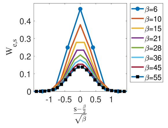
Figure C.1. Complete graphs of $n$ vertices, with $n$ ranging from $5$ to $12$.

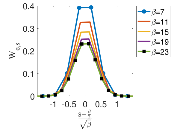
Figure C.2. Periodic ladder graphs of $n$ steps, with $n\in\{6,10,14,18,22\}$.

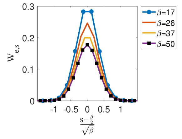
Figure C.3. Periodic square lattices of $n^{2}$ vertices for $n$ ranging between $4$ to $7$.

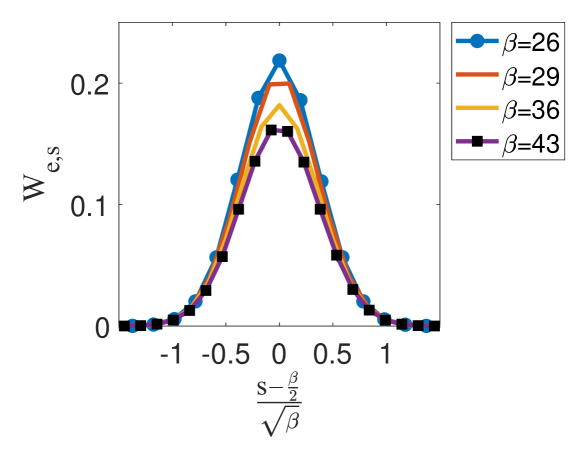
Figure C.4. Random Erdős-Rényi graphs with $n$ vertices and $p=0.75$, for $n$ ranging between $9$ to $12$.

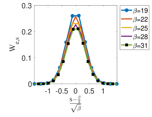
Figure C.5. Random $5$-regular graphs of $n$ vertices,
for $n\in\{12,14,16,18,20\}$. The $\beta$ value was computed for each graph as discussed in Remark 3.10.

References

- [1] S. Albeverio and P. Kurasov, Singular perturbations of differential operators: solvable Schrödinger-type operators, vol. 271, Cambridge University Press, 2000.
- [2] L. Alon, Generic laplace eigenfunctions on metric graphs, preprint, arXiv:2203.16111.
- [3] L. Alon, Quantum graphs - Generic eigenfunctions and their nodal count and Neumann count statistics, PhD thesis, Mathamtics Department, Technion - Israel Institute of Technology, 2020. arXiv:2010.03004.
- [4] L. Alon and R. Band, Neumann domains on quantum graphs, in Annales Henri Poincaré, vol. 22, Springer, 2021, pp. 3391–3454.
- [5] L. Alon, R. Band, and G. Berkolaiko, Nodal statistics on quantum graphs, Communications in Mathematical Physics, (2018).
- [6] R. Band, The nodal count implies the graph is a tree, Philos. Trans. R. Soc. Lond. A, 372 (2014), pp. 20120504, 24. preprint arXiv:1212.6710.
- [7] R. Band and G. Berkolaiko, Universality of the momentum band density of periodic networks, Phys. Rev. Lett., 111 (2013), p. 130404.
- [8] R. Band, G. Berkolaiko, and U. Smilansky, Dynamics of nodal points and the nodal count on a family of quantum graphs, Annales Henri Poincare, 13 (2012), pp. 145–184.
- [9] R. Band, J. Harrison, and M. Sepanski, Lyndon word decompositions and pseudo orbits on q-nary graphs, Journal of Mathematical Analysis and Applications, 470 (2019), pp. 135–144.
- [10] R. Band, I. Oren, and U. Smilansky, Nodal domains on graphs—how to count them and why?, in Analysis on graphs and its applications, vol. 77 of Proc. Sympos. Pure Math., Amer. Math. Soc., Providence, RI, 2008, pp. 5–27.
- [11] F. Barra and P. Gaspard, On the level spacing distribution in quantum graphs, J. Statist. Phys., 101 (2000), pp. 283–319.
- [12] D. Beliaev and Z. Kereta, On the bogomolny–schmit conjecture, Journal of Physics A: Mathematical and Theoretical, 46 (2013), p. 455003.
- [13] D. Beliaev, M. McAuley, and S. Muirhead, On the number of excursion sets of planar Gaussian fields, Probab. Theory Related Fields, 178 (2020), pp. 655–698.
- [14] G. Berkolaiko, A lower bound for nodal count on discrete and metric graphs, Comm. Math. Phys., 278 (2008), pp. 803–819.
- [15] , Nodal count of graph eigenfunctions via magnetic perturbation, Anal. PDE, 6 (2013), pp. 1213–1233. preprint arXiv:1110.5373.
- [16] G. Berkolaiko, J. P. Keating, and B. Winn, No quantum ergodicity for star graphs, Comm. Math. Phys., 250 (2004), pp. 259–285.
- [17] G. Berkolaiko and P. Kuchment, Introduction to Quantum Graphs, vol. 186 of Mathematical Surveys and Monographs, AMS, 2013.
- [18] G. Berkolaiko and W. Liu, Simplicity of eigenvalues and non-vanishing of eigenfunctions of a quantum graph, J. Math. Anal. Appl., 445 (2017), pp. 803–818. preprint arXiv:1601.06225.
- [19] G. Berkolaiko and T. Weyand, Stability of eigenvalues of quantum graphs with respect to magnetic perturbation and the nodal count of the eigenfunctions, Philos. Trans. R. Soc. Lond. Ser. A Math. Phys. Eng. Sci., 372 (2014), pp. 20120522, 17.
- [20] G. Berkolaiko and B. Winn, Relationship between scattering matrix and spectrum of quantum graphs, Trans. Amer. Math. Soc., 362 (2010), pp. 6261–6277.
- [21] G. Blum, S. Gnutzmann, and U. Smilansky, Nodal domains statistics: A criterion for quantum chaos, Phys. Rev. Lett., 88 (2002), p. 114101.
- [22] E. Bogomolny and C. Schmit, Percolation Model for Nodal Domains of Chaotic Wave Functions, Physical Review Letters, 88 (2002), p. 114102.
- [23] Y. Colin de Verdière, Spectres de graphes, vol. 4 of Cours Spécialisés [Specialized Courses], Société Mathématique de France, Paris, 1998.
- [24] , Magnetic interpretation of the nodal defect on graphs, Anal. PDE, 6 (2013), pp. 1235–1242. preprint arXiv:1201.1110.
- [25] Y. Colin de Verdière, Semi-classical measures on quantum graphs and the Gauß map of the determinant manifold, Annales Henri Poincaré, 16 (2015), pp. 347–364. also arXiv:1311.5449.
- [26] R. Courant, Ein allgemeiner Satz zur Theorie der Eigenfunktione selbstadjungierter Differentialausdrücke, Nach. Ges. Wiss. Göttingen Math.-Phys. Kl., (1923), pp. 81–84.
- [27] R. Courant and D. Hilbert, Methods of mathematical physics. Vol. I, Interscience Publishers, Inc., New York, N.Y., 1953.
- [28] G. Cox, C. K. R. T. Jones, and J. L. Marzuola, Manifold decompositions and indices of Schrödinger operators, Indiana Univ. Math. J., 66 (2017), pp. 1573–1602.
- [29] E. B. Davies, G. M. L. Gladwell, J. Leydold, and P. F. Stadler, Discrete nodal domain theorems, Linear Algebra Appl., 336 (2001), pp. 51–60.
- [30] P. Exner and O. r. Turek, Periodic quantum graphs from the Bethe-Sommerfeld perspective, J. Phys. A, 50 (2017), pp. 455201, 32.
- [31] S. Gnutzmann and A. Altland, Spectral correlations of individual quantum graphs, Phys. Rev. E (3), 72 (2005), pp. 056215, 14.
- [32] S. Gnutzmann and U. Smilansky, Quantum graphs: Applications to quantum chaos and universal spectral statistics, Adv. Phys., 55 (2006), pp. 527–625.
- [33] S. Gnutzmann, U. Smilansky, and J. Weber, Nodal counting on quantum graphs, Waves Random Media, 14 (2004), pp. S61–S73.
- [34] J. Harrison and T. Hudgins, Complete dynamical evaluation of the characteristic polynomial of binary quantum graphs. preprint arXiv:2011.05213, 2020.
- [35] M. Hofmann, J. B. Kennedy, D. Mugnolo, and M. Plümer, On Pleijel’s nodal domain theorem for quantum graphs, in Annales Henri Poincaré, vol. 22, Springer, 2021, pp. 3841–3870.
- [36] T. Kato, Perturbation theory for linear operators, Springer-Verlag, Berlin, second ed., 1976. Grundlehren der Mathematischen Wissenschaften, Band 132.
- [37] M. Keller and M. Schwarz, Courant’s nodal domain theorem for positivity preserving forms, J. Spectr. Theory, 10 (2020), pp. 271–309.
- [38] A. J. Kollár and P. Sarnak, Gap sets for the spectra of cubic graphs, arXiv preprint arXiv:2005.05379, (2020).
- [39] K. Konrad, Asymptotic statistics of nodal domains of quantum chaotic billiards in the semiclassical limit. Senior Thesis Dartmouth College, 2012.
- [40] T. Kottos and U. Smilansky, Quantum chaos on graphs, Phys. Rev. Lett., 79 (1997), pp. 4794–4797.
- [41] , Periodic orbit theory and spectral statistics for quantum graphs, Ann. Physics, 274 (1999), pp. 76–124.
- [42] C. Léna, Pleijel’s nodal domain theorem for Neumann and Robin eigenfunctions, Annales de l’Institut Fourier, 69 (2019), pp. 283–301.
- [43] D. Mugnolo, Semigroup methods for evolution equations on networks, Understanding Complex Systems, Springer, Cham, 2014.
- [44] M. Nastasescu, The number of ovals of a random real plane curve. Senior Thesis Princeton University, 2011.
- [45] F. Nazarov and M. Sodin, On the number of nodal domains of random spherical harmonics, Amer. J. Math., 131 (2009), pp. 1337–1357.
- [46] F. Nazarov and M. Sodin, Asymptotic laws for the spatial distribution and the number of connected components of zero sets of gaussian random functions, Journal of Mathematical Physics, Analysis, Geometry, 12 (2016), pp. 205–278.
- [47] , Fluctuations in the number of nodal domains, J. Math. Phys., 61 (2020), pp. 123302, 39.
- [48] R. Phillips and P. Sarnak, Geodesics in homology classes, Duke Mathematical Journal, 55 (1987), pp. 287–297.
- [49] Å. Pleijel, Remarks on Courant’s nodal line theorem, Comm. Pure Appl. Math., 9 (1956), pp. 543–550.
- [50] I. Polterovich, Pleijel’s nodal domain theorem for free membranes, Proc. Amer. Math. Soc., 137 (2009), pp. 1021–1024.
- [51] F. Rellich and J. Berkowitz, Perturbation theory of eigenvalue problems, CRC Press, 1969.
- [52] K. Schmüdgen, Unbounded self-adjoint operators on Hilbert space, vol. 265 of Graduate Texts in Mathematics, Springer, Dordrecht, 2012.
- [53] G. Tanner, Unitary-stochastic matrix ensembles and spectral statistics, J. Phys. A, 34 (2001), pp. 8485–8500.
- [54] J. von Below, A characteristic equation associated to an eigenvalue problem on -networks, Linear Algebra Appl., 71 (1985), pp. 309–325.