Sparse Bayesian Learning via Stepwise Regression

Abstract

Sparse Bayesian Learning (SBL) is a powerful framework for attaining sparsity in probabilistic models. Herein, we propose a coordinate ascent algorithm for SBL termed Relevance Matching Pursuit (RMP) and show that, as its noise variance parameter goes to zero, RMP exhibits a surprising connection to Stepwise Regression. Further, we derive novel guarantees for Stepwise Regression algorithms, which also shed light on RMP. Our guarantees for Forward Regression improve on deterministic and probabilistic results for Orthogonal Matching Pursuit with noise. Our analysis of Backward Regression on determined systems culminates in a bound on the residual of the optimal solution to the subset selection problem that, if satisfied, guarantees the optimality of the result. To our knowledge, this bound is the first that can be computed in polynomial time and depends chiefly on the smallest singular value of the matrix. We report numerical experiments using a variety of feature selection algorithms. Notably, RMP and its limiting variant are both efficient and maintain strong performance with correlated features.

1 Introduction

Finding a sparse solution to underdetermined linear systems is a fundamental problem in a diverse array of domains and applications, like network systems (Haupt et al., , 2008), materials science (Szameit et al., , 2012), medical imaging (Lustig et al., , 2007), and more. The problem can be formalized as

$$\min\|\mathbb{x}\|_{0}\ \ \text{ s.t. }\ \ \boldsymbol{\Phi}\mathbb{x}=\mathbb{y},$$ (1.1)

where $\boldsymbol{\Phi}\in\mathbb{R}^{n\times m}$ is a matrix with potentially more columns than rows, $\mathbb{y}$ is the observation we are trying to represent using an unknown sparse vector $\mathbb{x}$, and $\|\mathbb{x}\|_{0}$ stands for the number of non-zero elements in $\mathbb{x}$. A column $\boldsymbol{\varphi}_{i}$ of $\boldsymbol{\Phi}$ is variously referred to as a feature or an atom. This problem has been studied extensively, resulting in myriad existing methods and algorithms.

In the present work, we study two seemingly disparate techniques for solving problem (1.1): Sparse Bayesian Learning (SBL) and Stepwise Regression. SBL is based on the Automatic Relevance Determination (ARD) framework (MacKay, 1992a, ; MacKay, 1992b, ) and is concerned with a generative model of the form

$$\boldsymbol{\Phi}\mathbb{x}=\mathbb{y}+\boldsymbol{\epsilon},$$ (1.2)

where $\boldsymbol{\Phi}$ is a deterministic matrix, $\epsilon_{i}\sim\mathcal{N}(0,\sigma)$ are independent noise variables, and the prior distribution over the coefficients is $x_{i}\sim\mathcal{N}(0,\gamma_{i})$ (Tipping, , 2001). Each coefficient has an independent prior variance $\gamma_{i}$, the defining characteristic of the ARD prior. Sparse Bayesian models are usually trained via type-II maximum likelihood estimation, which is the maximization of the marginal likelihood with respect to $\boldsymbol{\gamma}$. The logarithm of the marginal likelihood is

$$\mathcal{L}(\boldsymbol{\gamma}) \overset{\text{\tiny{def}}}{=}\log\int p(\mathbb{y}|\mathbb{x})p(\mathbb{x}|\boldsymbol{\gamma})d\mathbb{x}$$ (1.3)

$$=-\mathbb{y}^{*}{\mathbb{C}^{-1}}\mathbb{y}-\log|{\mathbb{C}}|-n\log(2\pi),$$

where ${\mathbb{C}}\overset{\text{\tiny{def}}}{=}(\sigma^{2}\mathbb{I}+\boldsymbol{\Phi}\boldsymbol{\Gamma}\boldsymbol{\Phi}^{*})$, and $\boldsymbol{\Gamma}\overset{\text{\tiny{def}}}{=}\text{diag}(\boldsymbol{\gamma})$. Since every coefficient has its own prior variance, the optimization effectively prunes extraneous features of $\boldsymbol{\Phi}$ if their prior variances approache zero. Since this provably happens frequently (Wipf and Rao, , 2005), ARD and SBL are powerful tools for promoting sparsity in a variety of applications.

Stepwise Regression, on the other hand, is a class of well-known greedy algorithms that add and delete features from a candidate solution based on two rules:

$$\arg\min_{i\not\in\mathcal{A}}\|\mathbb{r}_{\mathcal{A}\cup i}\|_{2},\qquad\text{and}\qquad\arg\min_{i\in\mathcal{A}}\|\mathbb{r}_{\mathcal{A}\backslash i}\|_{2},$$ (1.4)

where $\mathbb{r}_{\mathcal{A}}$ is the least-squares residual using only features indexed by $\mathcal{A}$. The intuitive appeal and practical performance of these greedy heuristics have led separate communities to rediscover the same algorithms, leading to a bewildering number of names. The algorithm that selects features based on the left side of (1.4) is known as Forward Regression, Forward Selection (Miller, , 2002), Order-Recursive Matching Pursuit (ORMP) (Cotter et al., , 1999), Optimized Orthogonal Matching Pursuit (Rebollo-Neira and Lowe, , 2002), and Orthogonal Least-Squares (Cotter et al., , 1999). The algorithm that eliminates features based on the right side of (1.4) is known as Backward Regression, Backward Elimination (Miller, , 2002), and Backward Optimized Orthogonal Matching Pursuit (Andrle et al., , 2004). Unless otherwise noted, we will refer to them simply as the forward and backward algorithm, respectively.

Contributions

We propose Relevance Matching Pursuit (RMP_σ), an algorithm which simultaneously maximizes (1.3) locally, and exhibits a surprising relationship to Stepwise Regression. Indeed, by analyzing RMP_σ in the noiseless limit in Section 3, we derive RMP₀, a combination of the well-known forward and backward algorithms. Having established this connection, we derive novel theoretical guarantees for Stepwise Regression on noisy data in Section 4. The guarantees for Forward Regression improve on existing deterministic and probabilistic results for Orthogonal Matching Pursuit. The bounds of the tolerable perturbation for Backward Regression are, to our knowledge, the first that can be computed in polynomial time and provide an important insight: the backward algorithm returns the optimal solution to the subset selection problem on a determined linear system, as long as the residual of the solution is bounded by a quantity that is proportional to the smallest singular value of the matrix. We experimentally verify our prediction that RMP₀ exhibits comparable support recovery performance to RMP_σ and compare against some of the most potent feature selection algorithms in Section 5. The results demonstrate RMP’s combination of performance and efficiency, corroborating our theoretical analysis. The only method with a consistent performance advantage over RMP_σ and RMP₀ is the ARD-based reweighted $l_{1}$-norm minimization of Wipf and Nagarajan, (2008), though the approach is computationally substantially more expensive.

2 Relevant Work

Given the vast amount of work on sparsity-inducing methods, we focus on the most relevant to ours. In the following, we will use the bra-ket notation $\langle\mathbb{\cdot}|\cdot\rangle$ to denote an inner product. A feature that has been selected by an algorithm is considered active and we refer to the set $\mathcal{A}$ of all active features as the active set.

Basis Pursuit

Basis Pursuit (BP) is a framework for solving (1.1) via the following convex relaxation:

$$\min\|\mathbb{x}\|_{1}\ \ \text{ s.t. }\ \ \boldsymbol{\Phi}\mathbb{x}=\mathbb{y}.$$ (2.1)

Under certain assumptions on the matrix $\boldsymbol{\Phi}$ and the sparsity level $k=\|\mathbb{x}\|_{0}$, (2.1) has the same global optimum as (1.1) (Chen et al., , 2001; Candès et al., , 2006). An important modification to BP for noisy observations is Basis Pursuit Denoising (BPDN) which replaces the equality constraint with $\|\boldsymbol{\Phi}\mathbb{x}-\mathbb{y}\|\leq\delta$, where $\delta$ is an upper bound on the perturbation of the signal (Chen et al., , 2001; Donoho and Elad, , 2006). This is closely related to the least absolute shrinkage and selection operator (LASSO) (Tibshirani, , 1996; Zhao and Yu, , 2007; Bach, , 2008). Cawley et al., (2007) studied this principle in the Bayesian framework, where the $l_{1}$-regularizer is equivalent to a Laplacian prior. Other notable algorithms based on relaxations of (1.1) include FOCUSS, an iterative least-squares scheme (Gorodnitsky and Rao, , 1997), and a reweighted $l_{1}$-norm minimization algorithm proposed in (Candes et al., , 2008), both approximating an entropic regularization term. While algorithms based on relaxations can offer strong sparse recovery guarantees and performance, they can be computationally expensive for large problems. Efficient greedy algorithms have been developed for this reason.

Matching Pursuit

An important family of greedy algorithms for (1.1) are Matching Pursuit (MP) and its variants (Mallat and Zhifeng Zhang, , 1993). Matching Pursuit updates a candidate solution one element at a time. The specific element $i$ is chosen by the rule $\arg\max_{i}|\langle\boldsymbol{\varphi}_{i}|\mathbb{r}\rangle|$, where $\boldsymbol{\varphi}_{i}$ is the $i$th column of $\boldsymbol{\Phi}$ and $\mathbb{r}=\mathbb{y}-\boldsymbol{\Phi}\mathbb{x}$ is the current residual. Orthogonal Matching Pursuit (OMP), also known as Stagewise Regression, uses the same rule to add features, but additionally optimizes all coefficients of the active set in each iteration:

$$\arg\max_{i}|\langle\boldsymbol{\varphi}_{i}|\mathbb{r}_{\mathcal{A}}\rangle|,$$ (2.2)

where $\mathbb{r}_{\mathcal{A}}$ is the least-squares residual given the set of atoms $\mathcal{A}$. Remarkably, OMP has theoretical guarantees for the problem of recovering the support of exactly sparse signals, even for noisy measurements (Davis et al., , 1997; Tropp, , 2004; Tropp and Gilbert, , 2007; Rangan and Fletcher, , 2009; Cai and Wang, , 2011). Recently, Matching Pursuits have served as inspiration for optimization algorithms: Tibshirani, (2015) proposed a general framework for stagewise algorithms with applications to group-structured learning, matrix completion, and image denoising. Locatello et al., (2018) developed a unified analysis of MP and coordinate ascent algorithms and Combettes and Pokutta, (2019) proposed Blended Matching Pursuit, combining coordinate descent and gradient steps to compute sparse minimizers of general convex objectives quickly.

Stepwise Regression

We here focus on known theoretical guarantees of the forward and backward algorithms and existing algorithms that combine them. Das and Kempe, (2018) proposed a notion of approximate submodularity and showed that it is satisfied by the coefficient of determination, $R^{2}$. In this way, they proved approximation guarantees of the forward algorithm and OMP to the optimal solution of the subset selection problem, which were generalized by Elenberg et al., (2018) for general convex objectives. Couvreur and Bresler, (2000) analyzed the backward algorithm and proved the existence of a bound on the perturbation magnitude that guarantees the recovery of the support of sparse solutions of linear systems.

Andrle et al., (2004) proposed running the forward and backward algorithm consecutively, but did not provide theoretical guarantees, nor empirical comparisons against other algorithms. Zhang, (2009) proposed FoBa, which combines both forward and backward heuristics into an adaptive algorithm. Similarly, Rao et al., (2015) proposed a forward-backward algorithm for the optimization of convex relaxations of (1.1) based on atomic norms and, most recently, Borboudakis and Tsamardinos, (2019) proposed an early-dropping heuristic for forward-backward algorithms for general feature selection problems.

Sparse Bayesian Learning

The first algorithms for the optimization of (1.3) for SBL were based on expectation-maximization (EM) updates and the fixed-point updates of MacKay (Tipping, , 2001). Though these methods are able to obtain sparse solutions to (1.2), they have no convergence guarantees and are slow for large problems, due to the at least quadratic scaling with the number of features (Tipping, , 2001). Wipf and Rao, (2004) showed how to adapt the EM-based SBL algorithm to the $l_{0}$-minimization problem (1.1) and proved that, in contrast to BP, the resulting optimization problem has the same global optimum as (1.1) and suffers from fewer local minima than competing non-convex relaxations. Subsequently, Wipf and Nagarajan, (2008) showed that the usual type-II approach can be interpreted as a type-I (MAP) approach with a special non-factorial prior. Using this insight, they proposed an algorithm based on reweighted $l_{1}$-norm minimization, which provably converges to a local maximum of the marginal likelihood, performs at least as well as BP in recovering sparse signals, and usually outperforms techniques based on $l_{1}$, $l_{2}$, and entropy regularization (Wipf and Nagarajan, , 2009), especially when dictionaries are structured and coherent (Wipf, , 2011).

3 Relevance Matching Pursuit

This section first recapitulates the derivation of the coordinate ascent updates for SBL derived by Tipping and Faul, (2003), subsequently introduces the Relevance Matching Pursuit algorithm, and analyzes the algorithm’s behavior as the noise variance approaches zero.

3.1 SBL via Coordinate Ascent

Recall from the introduction that ${\mathbb{C}}=(\sigma^{2}\mathbb{I}+\boldsymbol{\Phi}\boldsymbol{\Gamma}\boldsymbol{\Phi}^{*})$ is the covariance of the marginal distribution and $\boldsymbol{\Gamma}=\text{diag}(\boldsymbol{\gamma})$ is the prior variance of the weights $\mathbb{x}$. In the context of SBL, we refer to $\mathcal{A}=\{i|\gamma_{i}\neq 0\}$ as the active set. Following the analysis of Tipping and Faul, (2003) and based on the Woodbury matrix identity, we separate out the contribution of a single prior variance $\gamma_{i}$ to the marginal likelihood (1.3):

$$\mathcal{L}(\boldsymbol{\gamma}) =\mathcal{L}(\boldsymbol{\gamma}_{-i})+\frac{1}{2}\left(\frac{q_{i}^{2}}{\gamma_{i}^{-1}+s_{i}}-\log\frac{1}{1+\gamma_{i}s_{i}}\right)$$

$$=\mathcal{L}(\boldsymbol{\gamma}_{-i})+l(\gamma_{i}),$$

where $q_{i}\overset{\text{\tiny{def}}}{=}\boldsymbol{\varphi}_{i}\mathbb{C}_{\mathcal{A}\backslash i}^{-1}\mathbb{y}$ and $s_{i}\overset{\text{\tiny{def}}}{=}\boldsymbol{\varphi}_{i}\mathbb{C}_{\mathcal{A}\backslash i}^{-1}\boldsymbol{\varphi}_{i}$, also termed the "quality" and "sparsity" factors by Faul and Tipping, (2002). $\mathbb{C}_{\mathcal{A}\backslash i}$ is as in (1.3) but only includes the features $\boldsymbol{\varphi}_{k}$ and corresponding prior variances $\gamma_{k}$ for $k\in\mathcal{A}\backslash i$. Crucially, the argument of the maximum of the marginal likelihood with respect to a single prior variance $\gamma_{i}$ is unique and has a closed form:

$$\arg\max_{\gamma_{i}}\ l(\gamma_{i})=\begin{cases}(q_{i}^{2}-s_{i})/s_{i}^{2}&q_{i}^{2}>s_{i}\\ 0&\text{else}\end{cases}.$$ (3.1)

Equation (3.1) is the basis of the efficient coordinate ascent updates put forth in Tipping and Faul, (2003). Associated with each coordinate update is a change in the marginal likelihood. If $q_{i}^{2}>s_{i}$, we denote by $\Delta_{\text{add}}(i)$, respectively $\Delta_{\text{update}}(i)$, the change in the marginal likelihood corresponding to setting a $\gamma_{i}$ which was previously zero, respectively non-zero, via equation (3.1).

We now make two preliminary observations. Given a subset of features $\mathcal{A}$, and a noise variance $\sigma^{2}$, the posterior mean ${\boldsymbol{\mu}}_{\mathcal{A},\sigma}$ and variance $\boldsymbol{\Sigma}_{\mathcal{A},\sigma}$ of the subset of weights $\mathbb{x}_{\mathcal{A}}$ are given by

$$\boldsymbol{\Sigma}_{\mathcal{A},\sigma} =({\boldsymbol{\Gamma}_{\mathcal{A}}}^{-1}+\sigma^{-2}\boldsymbol{\Phi}_{\mathcal{A}}^{T}\boldsymbol{\Phi}_{\mathcal{A}})^{-1},$$

$${\boldsymbol{\mu}}_{\mathcal{A},\sigma} =\sigma^{-2}\boldsymbol{\Sigma}_{\mathcal{A}}\boldsymbol{\Phi}_{\mathcal{A}}^{*}\mathbb{y},$$

where $\boldsymbol{\Phi}_{\mathcal{A}}$ and $\boldsymbol{\Gamma}_{\mathcal{A}}$ are the submatrices of $\boldsymbol{\Phi}$ and $\boldsymbol{\Gamma}$ corresponding to $\mathcal{A}$. The Woodbury identity gives

$$\mathbb{R}_{\mathcal{A},\sigma} \overset{\text{\tiny{def}}}{=}\sigma^{2}\mathbb{C}^{-1}=\mathbb{I}-\boldsymbol{\Phi}_{\mathcal{A}}[\sigma^{-2}\boldsymbol{\Sigma}_{\mathcal{A}}]\boldsymbol{\Phi}_{\mathcal{A}}^{*},$$

and thus, $\mathbb{r}_{\mathcal{A},\sigma}\overset{\text{\tiny{def}}}{=}\mathbb{y}-\boldsymbol{\Phi}_{\mathcal{A}}{\boldsymbol{\mu}}_{\mathcal{A},\sigma}=\mathbb{R}_{\mathcal{A},\sigma}\mathbb{y}.$ We can now express the following result on the condition which leads SBL to include or exclude a feature.

Lemma 3.1.

The optimum of the marginal likelihood with respect to $\gamma_{i}$ occurs at a non-zero value if and only if

$$|\langle\tilde{\boldsymbol{\varphi}}_{i}|\mathbb{r}_{\mathcal{A}\backslash i,\sigma}\rangle|>\sigma,$$

where $\tilde{\boldsymbol{\varphi}}_{i}\overset{\text{\tiny{def}}}{=}\boldsymbol{\varphi}_{i}/\|\boldsymbol{\varphi}_{i}\|_{\mathbb{R}_{\mathcal{A}\backslash i,\sigma}}$, $\|\boldsymbol{\varphi}_{i}\|_{\mathbb{R}_{\mathcal{A}\backslash i,\sigma}}$ is the energetic norm $(\boldsymbol{\varphi}_{i}^{*}\mathbb{R}_{\mathcal{A}\backslash i,\sigma}\boldsymbol{\varphi}_{i})$ of $\boldsymbol{\varphi}_{i}$, and $\mathcal{A}$ is the active set.

Lemma 3.1 shows the direct and proportional dependency of the acquisition and deletion conditions on $\sigma$. The following result characterizes the inactive feature ($\gamma_{i}=0$) that leads to the maximal increase in the marginal likelihood upon its addition to the model.

Lemma 3.2.

Let $\Delta_{add}(i)$ be the change in the marginal likelihood upon setting an inactive feature’s prior variance $\gamma_{i}$ to its optimal value via equation (3.1). Then

$$\arg\max_{i\not\in\mathcal{A}}\Delta_{add}(i)=\arg\max_{i\not\in\mathcal{A}}|\langle\tilde{\boldsymbol{\varphi}}_{i}|\mathbb{r}_{\mathcal{A},\sigma}\rangle|.$$

where $\tilde{\boldsymbol{\varphi}}_{i}=\boldsymbol{\varphi}_{i}/\|\boldsymbol{\varphi}_{i}\|_{\mathbb{R}_{\mathcal{A},\sigma}}$, and $\mathcal{A}$ is the active set.

By comparing the right side of the equation in Lemma 3.2 to the acquisition criterion of OMP in (2.2), we see that a feature selection strategy based on the maximal increase in the marginal likelihood is intimately related to the family of Matching Pursuit algorithms. This serves as the inspiration for the name of Relevance Matching Pursuit (RMP), described in the next section.

3.2 Algorithm Design

In describing the coordinate ascent updates, Tipping and Faul, (2003) purposefully left several choices open: which variance $\gamma_{i}$ does the algorithm choose to update, add, or delete? In which order should these operations proceed? RMP arises from a particular choice for these design questions, enabling our analysis of the algorithm’s behavior, and proving to be closely related to Stepwise Regression. The design principles give rise to Algorithm 1 and are as follows:

1. Add features based on $\arg\max_{i\not\in\mathcal{A}}|\langle\tilde{\boldsymbol{\varphi}}_{i}|\mathbb{r}\rangle|$, until there is no inactive feature with $|\langle\tilde{\boldsymbol{\varphi}}_{i}|\mathbb{r}\rangle|~{}>~{}\sigma$ left.

2. Remove features based on $\arg\min_{i\not\in\mathcal{A}}|\langle\tilde{\boldsymbol{\varphi}}_{i}|\mathbb{r}\rangle|$, as long as there is a feature with $|\langle\tilde{\boldsymbol{\varphi}}_{i}|\mathbb{r}\rangle|\leq\sigma$.

3. Update the prior variance of the currently active atom whose update leads to the largest increase in the marginal likelihood, as long as there is a feature with $\Delta_{\text{update}}(i)>\delta_{\mathcal{L}}$, where $\delta_{\mathcal{L}}$ is an input to the algorithm and defines a convergence criterion.

Algorithm 1 Relevance Matching Pursuit (RMP_σ)

1:  Input: Dictionary $\boldsymbol{\Phi}$, signal $\mathbb{y}$, noise variance $\sigma^{2}$, convergence criterion $\delta_{\mathcal{L}}$

2:  Ouput: Support set $\mathcal{A}$, prior variances $\gamma_{i}$

3:  Initialize $\mathcal{A}\leftarrow\varnothing$

4:  Initialize $\gamma_{i}\leftarrow 0$ for all $i$

5:  while has not converged do

6:     while $\exists i\not\in\mathcal{A}$ s.t. $|\langle\tilde{\boldsymbol{\varphi}}_{i}|\mathbb{r}_{\mathcal{A},\sigma}\rangle|>\sigma$ do

7:        $i^{*}\leftarrow\arg\max_{i\not\in\mathcal{A}}|\langle\tilde{\boldsymbol{\varphi}}_{i}|\mathbb{r}_{\mathcal{A},\sigma}\rangle|$ {selection}

8:        $\mathcal{A}\leftarrow\mathcal{A}\cup i^{*}$ {add to active set}

9:        update $\gamma_{i^{*}}$ {set $\gamma_{i^{*}}$ via (3.1)}

10:     end while

11:     while true do

12:        if $\exists i\in\mathcal{A}$ s.t. $|\langle\tilde{\boldsymbol{\varphi}}_{i}|\mathbb{r}_{\mathcal{A}\backslash i,\sigma}\rangle|\leq\sigma$  then

13:           $i^{*}\leftarrow\arg\min_{i\in\mathcal{A}}|\langle\tilde{\boldsymbol{\varphi}}_{i}|\mathbb{r}_{\mathcal{A}\backslash i,\sigma}\rangle|$

14:           $\mathcal{A}\leftarrow\mathcal{A}\backslash i^{*}$ {elimination}

15:        else if $\exists i$ s.t. $\Delta_{\text{update}}(i)>\delta_{\mathcal{L}}$ then

16:           $i^{*}\leftarrow\arg\max_{i\in\mathcal{A}}\Delta_{\text{\tiny update}}(i)$ {update}

17:        else

18:           break

19:        end if

20:        update $\gamma_{i^{*}}$ {set $\gamma_{i^{*}}$ via (3.1)}

21:     end while

22:  end while

In Algorithm 1, we left the condition of the outer loop imprecise for a reason: in addition to terminating after an improvement to the likelihood fails to exceed $\delta_{\mathcal{L}}$ and no feature is left to add or delete, an implementation might include additional criteria, like a maximum runtime, number of iterations, or change in $\boldsymbol{\gamma}$. We further note that the coordinate ascent updates to $\gamma_{i}$ do provably converge to a joint maximum, not merely a stationary point (Faul and Tipping, , 2002). These facts imply

Lemma 3.3.

As $\delta_{\mathcal{L}}\to 0$, the $\boldsymbol{\gamma}$ returned by RMP_σ constitutes a local maximum of the marginal likelihood.

3.3 The Noiseless Limit

We now analyze the algorithm’s behavior as the noise variance $\sigma^{2}$ approaches zero. On a high level, this is analogous to the approach of Wipf and Rao, (2004, 2005) who studied the noiseless limit of the EM-updates for SBL. We make use of the following property of the Moore-Penrose inverse.

Lemma 3.4.

Assume the columns of $\boldsymbol{\Phi}_{\mathcal{A}}$, are linearly independent. Then

$$\mathbb{R}_{\mathcal{A}}\overset{\text{\tiny{def}}}{=}(\mathbb{I}-\boldsymbol{\Phi}_{\mathcal{A}}\boldsymbol{\Phi}_{\mathcal{A}}^{+})=\lim_{\sigma\to 0^{+}}\mathbb{R}_{\mathcal{A},\sigma}.$$

Note that $\mathbb{r}_{\mathcal{A}}=\mathbb{R}_{\mathcal{A}}\mathbb{y}$ is the ordinary least-squares residual of the active features $\boldsymbol{\Phi}_{\mathcal{A}}$ and $\mathbb{y}$. The following technical result is crucial in establishing the connection of RMP_σ to Stepwise Regression.

Lemma 3.5.

Let $\mathbb{r}_{\mathcal{A}}$ be the least-squares residual associated with a feature set $\mathcal{A}$. Then

$$\|\mathbb{r}_{\mathcal{A}}\|_{2}^{2}-\|\mathbb{r}_{\mathcal{A}\cup i}\|_{2}^{2} =|\langle\boldsymbol{\varphi}_{i},\mathbb{r}_{\mathcal{A}}\rangle|^{2}/\|\boldsymbol{\varphi}_{i}\|_{\mathbb{R}_{\mathcal{A}}}^{2},\text{and}$$ (3.2)

$$\|\mathbb{r}_{\mathcal{A}\backslash i}\|_{2}^{2}-\|\mathbb{r}_{\mathcal{A}}\|_{2}^{2} =|\langle\boldsymbol{\varphi}_{i},\mathbb{r}_{\mathcal{A}}\rangle|^{2}/\|\boldsymbol{\varphi}_{i}\|_{\mathbb{R}_{\mathcal{A}\backslash i}}^{2}.$$

An immediate corollary of Lemma 3.5 is that $\arg\min_{i}\|\mathbb{r}_{\mathcal{A}\cup i}\|=\arg\max_{i}|\boldsymbol{\varphi}_{i}\cdot\mathbb{r}_{\mathcal{A}}|/\|\boldsymbol{\varphi}_{i}\|_{\mathbb{R}_{\mathcal{A}}}$, and a similar expression for the second equation in (3.2). As Lemma 3.4 implies that the addition criteria of RMP_σ converge to the right-hand side of this expression, the criteria in fact converge to the ones of the forward and backward algorithm in equation (1.4).

It remains to study what happens to the prior-variance-update step in line 16 of Algorithm 1. Notably, $\mathbb{R}_{\mathcal{A}}$ is independent of $\boldsymbol{\Gamma}$ under the assumption of Lemma 3.4, and thus, so are the addition and deletion criteria of RMP_σ in this limit. Therefore, updating and keeping track of $\boldsymbol{\Gamma}$ is irrelevant for the execution of the algorithm if the active set is linearly independent.

This observation gives rise to Algorithm 2, which we term RMP₀, which models RMP_σ when there are no linearly dependent column in the active set. This is not a restrictive assumption since RMP₀ starts with an empty $\mathcal{A}$ and stops adding columns when a feasible solution is found since then $\mathbb{r}_{\mathcal{A}}=0$, which happens at the latest when $n$ columns are added. Inspired by the acquisition criterion in Lemma 3.1, we introduce an acquisition and deletion threshold $\delta$ separate from $\sigma$ to Algorithm 2, which makes the algorithm capable of handling noise. Setting $\delta\leftarrow 0$ corresponds to the noiseless limit of RMP_σ.

Algorithm 2 RMP₀

1:  Input: Dictionary $\boldsymbol{\Phi}$, signal $\mathbb{y}$, tolerance $\delta$

2:  Result: Support set $\mathcal{A}$

3:  Initialize $\mathcal{A}\leftarrow\varnothing$

4:  while has not converged do

5:     while $\exists i\in\mathcal{A}$ s.t. $\|\mathbb{r}_{\mathcal{A}}\|^{2}-\|\mathbb{r}_{\mathcal{A}\cup i}\|^{2}>\delta^{2}$ do

6:        $i^{*}\leftarrow\arg\max_{i\not\in\mathcal{A}}\|\mathbb{r}_{\mathcal{A}\cup i}\|$ {selection}

7:        $\mathcal{A}\leftarrow\mathcal{A}\cup i^{*}$

8:     end while

9:     while $\exists i\in\mathcal{A}$ s.t. $\|\mathbb{r}_{\mathcal{A}\backslash i}\|^{2}-\|\mathbb{r}_{\mathcal{A}}\|^{2}\leq\delta^{2}$ do

10:        $i^{*}\leftarrow\arg\min_{i\in\mathcal{A}}\|\mathbb{r}_{\mathcal{A}\backslash i}\|$ {elimination}

11:        $\mathcal{A}\leftarrow\mathcal{A}\backslash i^{*}$

12:     end while

13:  end while

4 Stepwise Regression

Having exposed a connection of Relevance Matching Pursuit to Stepwise Regression, we now provide novel theoretical insights about the forward and backward algorithms. To this end, we briefly introduce necessary theoretical tools.

4.1 Theoretical Preliminaries

Prior work has established that the performance of many feature selection and sparse recovery algorithms is highly dependent on the correlation of different features. The following definition quantifies this notion.

Definition 4.1 (Coherence).

The coherence $\mu$ of a matrix $\boldsymbol{\Phi}$, whose columns have unit norm, is defined as

$$\mu\overset{\text{\tiny{def}}}{=}\max_{i\neq j}|\langle\boldsymbol{\varphi}_{i}|\boldsymbol{\varphi}_{j}\rangle|.$$

The coherence is a measure of the orthogonality of $\boldsymbol{\Phi}$. It can lead to pessimistic estimates, as it only considers the maximal inner product of two columns. Tropp, (2004) introduced the Babel function to generalize the coherence by measuring the maximal sum of absolute inner products between a column and a set of columns. Its name is inspired by the Tower of Babel, since the function measures "how much the atoms are speaking the same language", and it can be used to derive sharper results.

Definition 4.2 (Babel Function).

The Babel function $\mu_{1}$ of a dictionary $\boldsymbol{\Phi}$ is defined as

$$\mu_{1}(k)\overset{\text{\tiny{def}}}{=}\max_{|\mathcal{I}|=k}\max_{i\not\in\mathcal{I}}\ \sum_{j\in\mathcal{I}}\ |\langle\boldsymbol{\varphi}_{i}|\boldsymbol{\varphi}_{j}\rangle|.$$

Notably, $\mu_{1}(1)=\mu$ and $\mu_{1}(k)\leq\mu k$ (Tropp, , 2004).

Using this notion, Tropp, (2004) proved that a necessary and sufficient condition for Orthogonal Matching Pursuit to recover any $k$-sparse vector is the Exact Recovery Condition.

Theorem 4.3 (Tropp, (2004)).

Orthogonal Matching Pursuit and Basis Pursuit succeed in recovering the support $\mathcal{S}$ of a $k$-sparse $\mathbb{x}$ from $\mathbb{y}=\boldsymbol{\Phi}\mathbb{x}$ if

$$\max_{j\not\in\mathcal{S}}\ \|\boldsymbol{\Phi}_{\mathcal{S}}^{+}\boldsymbol{\varphi}_{j}\|_{1}<1.$$

Further, this holds if $\mu_{1}(k)<1/2$.

Soussen et al., (2013) used the connection of the forward algorithm and OMP that was exposed through Lemma 3.5 to jointly analyze the two algorithms, proving that the exact recovery criterion in Theorem 4.3 is necessary and sufficient for both algorithms to retrieve any sparse signal with no noise. In particular, for each algorithm, there is a sparse signal which cannot be recovered in $k$ steps, if the inequality doesn’t hold. In this sense, the recovery guarantee for the forward algorithm without noise cannot be improved. Tropp, (2004) further points out that even the condition on the Babel function is necessary for exact recovery.

4.2 Forward Regression

For the results in this subsection, assume that $\boldsymbol{\Phi}$ has $l_{2}$-normalized columns. In comparison to the work of Cai and Wang, (2011) on OMP with noise, our main theoretical contributions for the analysis of the forward algorithms are related to the necessary recovery condition on the Babel function, $\mu_{1}(k)<1/2$, and its implications. Our analysis leads to both tighter deterministic and probabilistic bounds on the tolerable noise magnitude.

Theorem 4.4.

Orthogonal Matching Pursuit and Forward Regression recover the support of a $k$-sparse vector in $k$ iterations provided the Babel function $\mu_{1}$ and the perturbation ${\boldsymbol{\epsilon}}$ of the target $\mathbb{y}$ satisfy

$$\frac{1-2\mu_{1}(k)}{\sqrt{2[1+\mu_{1}(k)]}}\min_{i\in\mathcal{S}}|x_{i}|\geq\|{\boldsymbol{\epsilon}}\|_{2}.$$

Theorem 4.4 allows for a non-zero amount of noise as long as $\mu_{1}(k)<1/2$, which is necessary even in the noiseless case. The tolerable magnitude increases with decreasing Babel function value, and is proportional to the magnitude of the smallest non-zero entry in $\mathbb{x}$. Compared to Thm. 10 of Bruckstein et al., (2009) and Thm. 1 of Cai and Wang, (2011), Thm. 4.4 applies to both OMP and Forward Regression (FR) and improves the factor of $2$ in both prior results to $\sqrt{2(1+\mu_{1}(k))}$. This allows up to around $40\%$ more noise while generalizing the results, and converges to $\sqrt{2}$ as $\mu\to 0$, the provably tightest constant even for orthogonal matrices. We also derived the following novel probabilistic guarantee for perturbations that are normally distributed.

Theorem 4.5.

Suppose ${\boldsymbol{\epsilon}}\sim\mathcal{N}(0,\sigma^{2}\mathbb{I}_{n})$, and let $\delta=[1/2-\mu_{1}(k)]\min_{i\in\mathcal{S}}|x_{i}|/\sigma>0$ and $d=\lceil m/k\rceil$. Orthogonal Matching Pursuit and Forward Regression recover the support of a $k$-sparse signal with probability exceeding

$$1-\left\lceil\frac{m}{k}\right\rceil\left(\frac{1+\kappa_{1}(k)}{1-\mu_{1}(2k)}\right)^{k/2}\left(1-\operatorname{erf}(\delta/\sqrt{2\kappa_{1}(k)})\right)^{k}.$$

where $\kappa_{1}(k)\overset{\text{\tiny{def}}}{=}(1+\mu_{1}(2k))/(1-\mu_{1}(k))$. For $\mu_{1}(2k)<1/2$, the result further holds with probability exceeding

$$1-\left\lceil\frac{m}{k}\right\rceil\left(\frac{4}{\sqrt{\pi}\delta}e^{-\delta^{2}/6}\right)^{k}.$$

By comparison, the existing bounds of Ben-Haim et al., (2010) and Cai and Wang, (2011) bound the probability of failure by $2me^{-\delta^{2}/2}/\delta$. Theorem 4.5 thus guarantees an earlier and much sharper phase transition (see Fig. 1). Critically, Theorem 4.5 makes use of the approximately isometric structure of subsets of columns of $\boldsymbol{\Phi}$, which is already inherent to the deterministic analysis, to derive a strong bound for $\|\boldsymbol{\Phi}^{*}{\boldsymbol{\epsilon}}\|$, for which prior works applied bounds for generic $\boldsymbol{\Phi}$. This allows us to apply much stronger multiplicative bounds since $\boldsymbol{\Phi}_{\mathcal{A}}^{*}{\boldsymbol{\epsilon}}$, an important quantity in the analysis, has an approximately diagonal covariance.

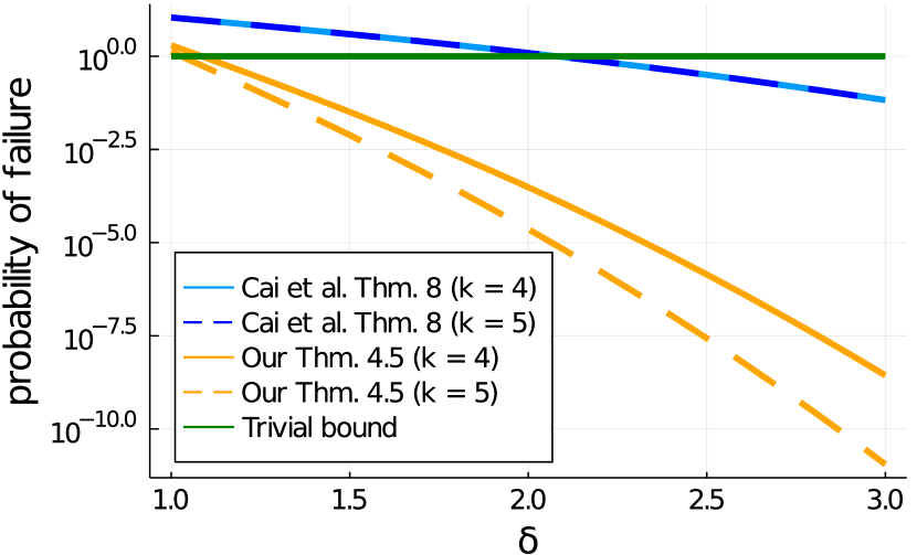
Figure 1: Comparing existing probabilistic bounds of (Cai and Wang, , 2011) to Theorem 4.5 for a matrix with $m=16$ columns, where $\delta=[1/2-\mu_{1}(k)]\min_{i\in\mathcal{S}}|x_{i}|/\sigma$.

Sparse Approximation and Exact Recovery

Elenberg et al., (2018) and Das and Kempe, (2018) provide elegant theoretical insights on the performance of OMP and FR. Both works present approximation guarantees, but do not provide exact recovery guarantees, as Theorems 4.4 and 4.5. The results are thus highly complementary; neither subsumes the other. To elaborate, their results for the $R^{2}$ score guarantee that FR’s result is at most a factor of $(1-e^{-\gamma})$ from the optimal value, where $\gamma=\sigma_{\min}^{2}(\boldsymbol{\Phi}_{\mathcal{S}})$. This is a strong result because it holds generally, even for non-sparse vectors and arbitrary noise. On the other hand, if $\gamma>1/2$ and a sparse vector generated the target with small noise, then Theorem 4.4 guarantees the exact recovery of the support, while the approximation guarantee with $\gamma~{}\approx~{}1/2$ only ensures FR to explain $\approx 40\%$ of the target variance.

4.3 Backward Regression

We now state our main optimality result for the backward algorithm. The existence of such a result was already proved in Couvreur and Bresler, (2000), though their bound is NP-hard to evaluate. In contrast, Theorem 4.6 reveals a proportional dependence of the tolerable noise on the smallest singular value of the matrix. While intuitive, this is to our knowledge the first result that makes this intuition precise.

Theorem 4.6.

Suppose $\boldsymbol{\Phi}$ has full column rank. Then Backward Regression recovers the support $\mathcal{S}$ of a $k$-sparse $m$-dimensional $\mathbb{x}$ in $m-k$ iterations if

$$\frac{\sigma_{\min}(\boldsymbol{\Phi})}{\sqrt{2[2-\sigma_{\min}(\boldsymbol{\Phi})^{2}]}}\min_{i\in\mathcal{S}}|x_{i}|>\|{\boldsymbol{\epsilon}}\|_{2},$$

where $\sigma_{\min}(\boldsymbol{\Phi})$ is the smallest singular value of $\boldsymbol{\Phi}$.

Remarkably, the Backward Regression (BR) only requires linear independence of the columns, which is implied by $\mu_{1}(k)<1$, but only applies to determined systems. Despite this necessarily stronger assumption, Thm. 4.6 is the first efficiently evaluable guarantee for this case. While the underdetermined case is most challenging, SBL is popularly applied to a kernel regression model for which the corresponding system is determined (see Sec. 5.4).

Still, because of this stronger assumption, it is important to connect the result for the backward algorithm with the already analyzed forward algorithm, the combination of which does apply to underdetermined systems. To this end, suppose a forward algorithm terminates with an arbitrary superset $\mathcal{A}$ of the true support, which is a weaker assumption than that of exact recovery. Then Theorem 4.6 applied to the submatrix $\boldsymbol{\Phi}_{\mathcal{A}}$ guarantees that the backward algorithm only deletes irrelevant features if the noise is not too large. The following corollary formalizes this idea.

Corollary 4.7.

Suppose $\boldsymbol{\Phi}_{\mathcal{A}}$ has full column rank, $|\mathcal{A}|=k$, and $\mathcal{S}\subset\mathcal{A}$. Then Backward Regression recovers the correct support $\mathcal{S}$ in $|\mathcal{A}|-|\mathcal{S}|$ iterations, provided

$$\sqrt{\frac{1-\mu_{1}(k)}{2[1+\mu_{1}(k)]}}\min_{i\in\mathcal{S}}|x_{i}|>\|{\boldsymbol{\epsilon}}\|_{2}.$$

Note the striking similarity of the bounds in Corollary 4.7 and Theorem 4.4, though the former is stronger. As Couvreur and Bresler, (2000) already established, the backward algorithm is not only capable of recovering the support of an exactly sparse vector, but in fact can solve the subset selection to optimality, provided the residual of the optimal solution is small enough. That is, for an arbitrary $\mathbb{y}$, not necessarily generated by $\boldsymbol{\Phi}\mathbb{x}$ with a sparse $\mathbb{x}$, we have

Theorem 4.8.

Let $\mathbb{x}_{k}$ be the vector that achieves the smallest residual norm $\|\mathbb{y}-\boldsymbol{\Phi}\mathbb{x}\|$ among all vectors $\mathbb{x}$ with $k$ or fewer non-zero elements. If the associated residual $\mathbb{r}_{k}\overset{\text{\tiny{def}}}{=}\mathbb{y}-\boldsymbol{\Phi}\mathbb{x}_{k}$ satisfies the bound in Theorem 4.6 in place of ${\boldsymbol{\epsilon}}$, Backward Regression recovers $\mathbb{x}_{k}$, or equivalently, solves the subset selection problem to optimality.

In an earlier short paper, we provided a precursory result for the backward algorithm (Ament and Gomes, , 2021). The full results we present herein provide tighter bounds and connect to the forward algorithm via Corollary 4.7. Similar to the results for the forward algorithm in the present work, the bound in Theorem 4.6 also converges to $\sqrt{2}$ as $\mu\to 0$, the provably tightest constant even for orthogonal matrices.

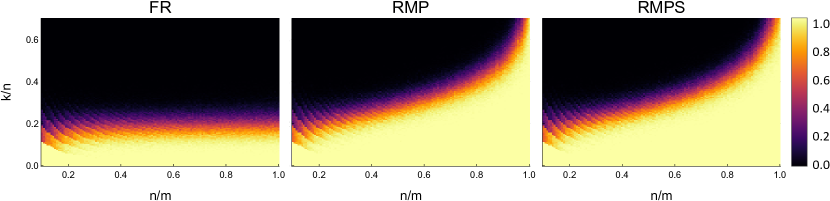
Figure 2: Empirical frequency of support recovery as a function of the sampling ratio $n/m$ and sparsity ratio $k/n$ for matrices with $m=128$ and $\|{\boldsymbol{\epsilon}}\|_{2}=10^{-2}$ for Forward Regression (left), RMP₀ (middle) and RMP_σ (right).

5 Numerical Experiments

The preceding results are powerful in their own right. Further, they guarantee that the backward stage of RMP₀ succeeds if the forward stage terminates with a superset of the true support, and the perturbation ${\boldsymbol{\epsilon}}$ is not too large. Therefore, we would expect RMP to have increasing support recovery performance as the sampling ratio $n/m$ increases. The validation of this hypothesis is the goal of our first experiment. Subsequently, we benchmark the recovery performance of a number of algorithms on uncorrelated and correlated features with noise, a kernel regression task, and end with a discussion of the experiments.

5.1 Setup and Implementation

Beside RMP, we implemented OMP, FR, FoBa (Zhang, , 2009), and the steepest coordinate ascent algorithm for SBL of Tipping and Faul, (2003) (FSBL). We compare two versions of RMP₀ in the experiments: RMP₀, and RMP₀+. The former denotes Algorithm 2 with only one iteration of the outer loop, while the latter terminates once the support stabilizes. We also compare against BPDN via constrained $l_{1}$-norm minimization, and the SBL-based reweighted $l_{1}$-norm algorithm of Wipf and Nagarajan, (2008) (BP ARD). We implemented all algorithms in Julia (Bezanson et al., , 2017), using the JuMP framework (Dunning et al., , 2017) to model the BP-approaches as second-order cone programs, and solve them using ECOS (Domahidi et al., , 2013) with default settings. All experiments were run on a workstation with an Intel Xeon CPU X5670 and 47 GB of memory.

For the synthetic experiments, the weights $\mathbb{x}$ are random $k$-sparse vectors with $\pm 1$ entries and the targets $\mathbb{y}$ were perturbed by random vectors distributed uniformly on the $10^{-2}$-hypersphere. For all algorithms, we input $\delta=2\|{\boldsymbol{\epsilon}}\|$ to simulate a small misspecification of the tolerance parameter that is likely to occur in practice. See also the supplementary materials for how RMP_σ could be adapted to infer the tolerance parameter, which however is a non-convex problem. Note that the stopping criteria of some of the algorithms depend differently on $\delta$: For OMP and BPDN, it is a constraint on the residual norm, for RMP₀, and FoBa, it is a bound on the marginal improvement in residual norm, and for RMP_σ, we assign $\sigma\rightarrow\delta$ and note that the stopping criterion depends on the more complex expression of Lemma 3.1.

Since the BP cone-programs do not directly return sparse solutions, we determine their support by dropping all entries below $\|{\boldsymbol{\epsilon}}\|/10$. In setting the threshold below the noise, we highlight that standard BPDN introduces a bias, while the ARD-based approach maintains the same global optimum as the $l_{0}$-minimization problem (Wipf and Nagarajan, , 2008). We stress that BP leads to sparse solutions in theory (Tropp, , 2006), but does not yield exactly sparse solutions using numerical LP-solvers, which terminate with many coefficients very close, but not equal to zero, necessitating the thresholding.

5.2 Phase-Transitions

First, we study the support recovery performance of Forward Regression (FR), RMP₀ and RMP_σ as a function of the sampling ratio $n/m$ of the matrix $\boldsymbol{\Phi}$ and the sparsity ratio $k/n$ of the weights $\mathbb{x}$. Figure 2 shows the empirical frequency of support recovery on column-normalized Gaussian random matrices with $m=128$ columns. Every cell is an average over 256 independent realizations of the experiment.

In accordance with the results for Stepwise Regression in Section 4, the recovery performance the RMP algorithms increases with the sampling ratio, since the likelihood that the forward stage recovers a superset of the true support increases. In contrast, the success of the forward algorithm in isolation is chiefly dependent on the sparsity ratio and apparently independent of $n/m$. The ridges in the bottom left of each plot are due to rounding effects since we set $k=\lceil(k/n)(n/m)m\rceil$. Importantly, the performance of RMP₀ is virtually identical to RMP_σ  and constitutes a first experimental validation of our analysis in Section 3.

5.3 Support Recovery with Noise

The following experiments have been established in the literature as a widespread proxy for performance on a variety of tasks, and thus allow for comparison to other reported results, for example those of Wipf and Rao, (2004), Candes et al., (2005, 2008), and He et al., (2017). In particular, we record the empirical frequency of support recovery of a large set of algorithms as a function of the sparsity level $k$ for two types of matrices. First, Gaussian random matrices and second, matrices generated as $\boldsymbol{\Phi}=\sum_{p}\frac{1}{p^{2}}\mathbb{u}\mathbb{v}^{*}$, where $\mathbb{u},\mathbb{v}$ have standard normal entries, inspired by the experiments in Xin et al., (2016). The two types of matrices exhibit low and high column correlations, respectively. We used matrices of size 64 by 128 and $l_{2}$-normalized the columns. The results reported in Tables 1 and 2 are averages over 1024 independent realizations with a 95% confidence interval below 0.02.

Table 1: Recovery probability for uncorrelated features

		Sparsity
Type	Algorithm	12	16	20	24
MP	OMP	$0.53$	$0.15$	$0.02$	$0.00$
	FR	$0.54$	$0.14$	$0.01$	$0.00$
	FoBa	$\bf 0.99$	$\bf 0.82$	$\bf 0.31$	$\bf 0.04$
	RMP0	$\bf 0.99$	$0.80$	$\bf 0.31$	$\bf 0.04$
	RMP0+	$\bf 0.99$	$0.80$	$\bf 0.31$	$\bf 0.04$
SBL	FSBL	$\bf 0.99$	$0.80$	$\bf 0.31$	$\bf 0.04$
	RMPσ	$\bf 0.99$	$\bf 0.81$	$\bf 0.31$	$\bf 0.04$
BP	BP	$0.26$	$0.05$	$0.01$	$0.00$
	BP ARD	$\bf 1.00$	$\bf 1.00$	$\bf 0.97$	$\bf 0.70$

Table 2: Recovery probability for correlated features

		Sparsity
Type	Algorithm	2	3	4	5
MP	OMP	$0.00$	$0.00$	$0.00$	$0.00$
	FR	$0.04$	$0.01$	$0.00$	$0.00$
	FoBa	$0.71$	$0.46$	$0.28$	$\bf 0.17$
	RMP0	$\bf 0.72$	$0.45$	$0.28$	$0.14$
	RMP0+	$\bf 0.72$	$\bf 0.48$	$\bf 0.32$	$\bf 0.17$
SBL	FSBL	$0.76$	$0.54$	$0.38$	$0.26$
	RMPσ	$\bf 0.81$	$\bf 0.58$	$\bf 0.45$	$\bf 0.30$
BP	BP	$0.02$	$0.00$	$0.00$	$0.00$
	BP ARD	$\bf 0.96$	$\bf 0.91$	$\bf 0.83$	$\bf 0.70$

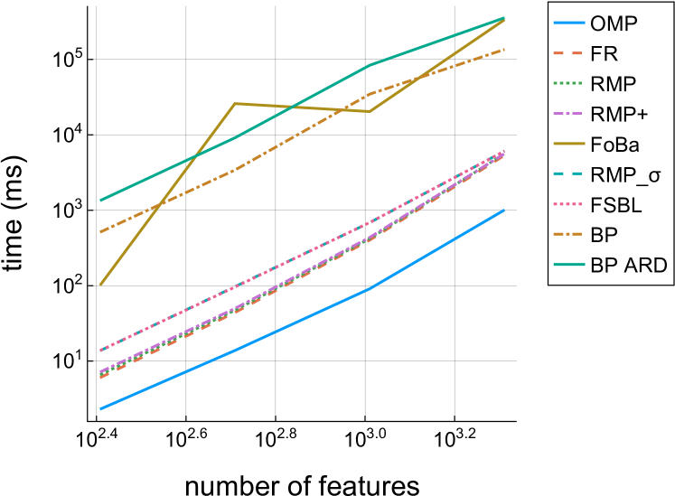
Figure 3: Timings for several algorithms on matrices with a fixed sampling ($1/2$) and sparsity ratio ($1/4$).

BP ARD demonstrates the best recovery performance among all tested methods, followed by RMP_σ. Importantly, RMP_σ exhibits similar performance to RMP₀ and virtually identical for uncorrelated features. The differences between RMP₀ and FoBa are marginal and plausibly attributable to statistical fluctuations. However, the differences in recovery performance of RMP_σ and FSBL is statistically significant for correlated features. BP performs poorly since our experiment was designed to expose that it does not preserve the same optimum as $l_{0}$-minimization.

Another notable approach is that of Koyejo et al., (2014), who proposed a greedy information-projection algorithm with applications to sparse estimation problems. In our study, the algorithm performed well on Gaussian matrices but deteriorated similarly to OMP and FR on coherent matrices, which is expected since it solely takes forward steps.

Figure 3 shows runtimes of the algorithms for matrices of increasing sizes. As $m$ increases, we kept the ratios $n/m=1/2$ and $k/m=1/4$. BP ARD is most time-consuming. RMP and RMP₀ are on average two orders of magnitude faster. The main performance difference between RMP_σ and RMP₀ comes from RMP_σ’s $\gamma_{i}$-update, which it can execute many times before converging. FoBa should in principle scale comparably to RMP₀, but doesn’t, as we chose not to let it take advantage of the efficient backward updates discussed in Reeves, (1999), but not mentioned in Zhang, (2009), which highlights their importance. Last, a limitation of the timings for BP are that we used generic LP solvers, while specialized algorithms exist (Beck and Teboulle, , 2009; Perez et al., , 2019) that can accelerate BP approaches. On the other hand, keeping the sparsity ratio $k/n$ fixed while growing $m$ is to the detriment of the greedy algorithms, which would need much fewer iterations if the sparsity level $k$ was fixed instead. In all, the timings are not designed to be fair but to illustrate the inevitable trade-off between performance and efficiency.

5.4 Sparse Kernel Regression

Following Tipping, (2001), we apply the SBL-related algorithms to a kernel regression model. In particular, given inputs $\{\mathbb{x}_{i}\}$, we assume the responses are generated according to $y\sim\mathcal{N}(f(\mathbb{x}),\sigma^{2})$, where

$$f(\mathbb{x})\ \overset{\text{\tiny{def}}}{=}\ \sum_{i}k(\mathbb{x},\mathbb{x}_{i})w_{i},$$ (5.1)

where $k$ is the Matérn-3/2 kernel and weights $w_{i}$. Given a training set, we optimize $w_{i}$ using the SBL-related algorithms, and evaluate on a test set using equation (5.1). Figure 4 shows the mean test error as a function of sparsity on the UCI Boston housing data (Dua and Graff, , 2017), which contains 506 data points. The results are averaged over 4608 sparsity-error values for each algorithm, generated by evaluations for different tolerance parameters $\delta$ (i.e. $\sigma$) and random 75-25 train-test splits. We conjecture that (F)SBL exhibits larger errors as it does not directly minimize squared errors, but instead the marginal likelihood. While FR can be competitive for highly sparse solutions, it is not as effective as RMP, RMP+ and FoBa, which achieve the best sparsity-error trade-off throughout all sparsity levels.

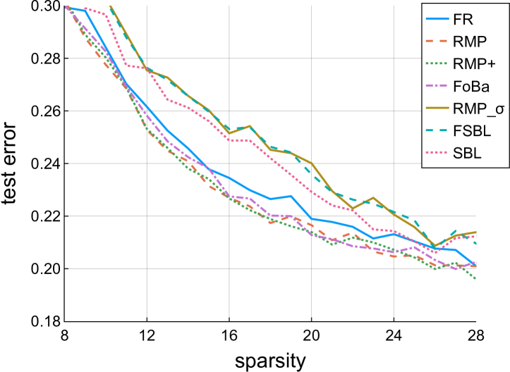
Figure 4: Test RMSE for a kernel regression model on the UCI Boston housing data as a function of achieved sparsity.

6 Conclusion

We proposed Relevance Matching Pursuit, a coordinate ascent algorithm for SBL whose analysis reveals a surprising connection to Stepwise Regression. The limiting algorithm RMP₀ closely tracks the performance of RMP_σ in our empirical evaluation, and is yet remarkably simple. We provided novel theoretical insights for Stepwise Regression, among them, an efficiently computable guarantee for the backward algorithm. Our results further provide theoretical justification to practitioners using Stepwise Regression in one of many statistics packages, prominently in the widely-used SAS. Finally, we hope these insights contribute to providing clarity in this vast space of the literature, and inspire further research on powerful sparsity-inducing algorithms.

References

- Ament and Gomes, (2021) Ament, S. and Gomes, C. (2021). On the optimality of backward regression: Sparse recovery and subset selection. In ICASSP 2021 - 2021 IEEE International Conference on Acoustics, Speech and Signal Processing (ICASSP), pages 5599–5603.
- Andrle et al., (2004) Andrle, M., Rebollo-Neira, L., and Sagianos, E. (2004). Backward-optimized orthogonal matching pursuit approach. IEEE Signal Processing Letters, 11(9):705–708.
- Bach, (2008) Bach, F. R. (2008). Consistency of the group lasso and multiple kernel learning. Journal of Machine Learning Research, 9(Jun):1179–1225.
- Beck and Teboulle, (2009) Beck, A. and Teboulle, M. (2009). A fast iterative shrinkage-thresholding algorithm for linear inverse problems. SIAM journal on imaging sciences, 2(1):183–202.
- Ben-Haim et al., (2010) Ben-Haim, Z., Eldar, Y. C., and Elad, M. (2010). Coherence-based performance guarantees for estimating a sparse vector under random noise. IEEE Transactions on Signal Processing, 58(10):5030–5043.
- Bezanson et al., (2017) Bezanson, J., Edelman, A., Karpinski, S., and Shah, V. B. (2017). Julia: A fresh approach to numerical computing. SIAM review, 59(1):65–98.
- Borboudakis and Tsamardinos, (2019) Borboudakis, G. and Tsamardinos, I. (2019). Forward-backward selection with early dropping. The Journal of Machine Learning Research, 20(1):276–314.
- Bruckstein et al., (2009) Bruckstein, A. M., Donoho, D. L., and Elad, M. (2009). From sparse solutions of systems of equations to sparse modeling of signals and images. SIAM review, 51(1):34–81.
- Cai and Wang, (2011) Cai, T. T. and Wang, L. (2011). Orthogonal matching pursuit for sparse signal recovery with noise. IEEE Transactions on Information Theory, 57(7):4680–4688.
- Candes et al., (2005) Candes, E., Rudelson, M., Tao, T., and Vershynin, R. (2005). Error correction via linear programming. In 46th Annual IEEE Symposium on Foundations of Computer Science (FOCS’05), pages 668–681. IEEE.
- Candès et al., (2006) Candès, E. J., Romberg, J., and Tao, T. (2006). Robust uncertainty principles: Exact signal reconstruction from highly incomplete frequency information. IEEE Transactions on information theory, 52(2):489–509.
- Candes et al., (2008) Candes, E. J., Wakin, M. B., and Boyd, S. P. (2008). Enhancing sparsity by reweighted l1 minimization. Journal of Fourier analysis and applications, 14(5-6):877–905.
- Cawley et al., (2007) Cawley, G. C., Talbot, N. L., and Girolami, M. (2007). Sparse multinomial logistic regression via bayesian l1 regularisation. In Advances in neural information processing systems, pages 209–216.
- Chen et al., (2001) Chen, S. S., Donoho, D. L., and Saunders, M. A. (2001). Atomic decomposition by basis pursuit. SIAM review, 43(1):129–159.
- Combettes and Pokutta, (2019) Combettes, C. and Pokutta, S. (2019). Blended matching pursuit. In Advances in Neural Information Processing Systems, pages 2042–2052.
- Cotter et al., (1999) Cotter, S. F., Adler, R., Rao, R. D., and Kreutz-Delgado, K. (1999). Forward sequential algorithms for best basis selection. IEE Proceedings - Vision, Image and Signal Processing, 146(5):235–244.
- Couvreur and Bresler, (2000) Couvreur, C. and Bresler, Y. (2000). On the optimality of the backward greedy algorithm for the subset selection problem. SIAM Journal on Matrix Analysis and Applications, 21(3):797–808.
- Das and Kempe, (2018) Das, A. and Kempe, D. (2018). Approximate submodularity and its applications: subset selection, sparse approximation and dictionary selection. The Journal of Machine Learning Research, 19(1):74–107.
- Davis et al., (1997) Davis, G., Mallat, S., and Avellaneda, M. (1997). Adaptive greedy approximations. Constructive approximation, 13(1):57–98.
- Domahidi et al., (2013) Domahidi, A., Chu, E., and Boyd, S. (2013). ECOS: An SOCP solver for embedded systems. In European Control Conference (ECC), pages 3071–3076.
- Donoho and Elad, (2006) Donoho, D. L. and Elad, M. (2006). On the stability of the basis pursuit in the presence of noise. Signal Processing, 86(3):511 – 532. Sparse Approximations in Signal and Image Processing.
- Dua and Graff, (2017) Dua, D. and Graff, C. (2017). UCI machine learning repository.
- Dunning et al., (2017) Dunning, I., Huchette, J., and Lubin, M. (2017). Jump: A modeling language for mathematical optimization. SIAM Review, 59(2):295–320.
- Elenberg et al., (2018) Elenberg, E. R., Khanna, R., Dimakis, A. G., Negahban, S., et al. (2018). Restricted strong convexity implies weak submodularity. The Annals of Statistics, 46(6B):3539–3568.
- Faul and Tipping, (2002) Faul, A. C. and Tipping, M. E. (2002). Analysis of sparse bayesian learning. In Advances in neural information processing systems, pages 383–389.
- Gorodnitsky and Rao, (1997) Gorodnitsky, I. F. and Rao, B. D. (1997). Sparse signal reconstruction from limited data using focuss: a re-weighted minimum norm algorithm. IEEE Transactions on Signal Processing, 45(3):600–616.
- Haupt et al., (2008) Haupt, J., Bajwa, W. U., Rabbat, M., and Nowak, R. (2008). Compressed sensing for networked data. IEEE Signal Processing Magazine, 25(2):92–101.
- He et al., (2017) He, H., Xin, B., Ikehata, S., and Wipf, D. (2017). From bayesian sparsity to gated recurrent nets. In Advances in Neural Information Processing Systems, pages 5554–5564.
- Koyejo et al., (2014) Koyejo, O. O., Khanna, R., Ghosh, J., and Poldrack, R. (2014). On prior distributions and approximate inference for structured variables. Advances in Neural Information Processing Systems, 27:676–684.
- Locatello et al., (2018) Locatello, F., Raj, A., Karimireddy, S. P., Raetsch, G., Schölkopf, B., Stich, S., and Jaggi, M. (2018). On matching pursuit and coordinate descent. In Dy, J. and Krause, A., editors, Proceedings of the 35th International Conference on Machine Learning, volume 80 of Proceedings of Machine Learning Research, pages 3198–3207, Stockholmsmässan, Stockholm Sweden. PMLR.
- Lustig et al., (2007) Lustig, M., Donoho, D., and Pauly, J. M. (2007). Sparse mri: The application of compressed sensing for rapid mr imaging. Magnetic Resonance in Medicine: An Official Journal of the International Society for Magnetic Resonance in Medicine, 58(6):1182–1195.
- (32) MacKay, D. J. (1992a). Bayesian interpolation. Neural computation, 4(3):415–447.
- (33) MacKay, D. J. (1992b). The evidence framework applied to classification networks. Neural computation, 4(5):720–736.
- Mallat and Zhifeng Zhang, (1993) Mallat, S. G. and Zhifeng Zhang (1993). Matching pursuits with time-frequency dictionaries. IEEE Transactions on Signal Processing, 41(12):3397–3415.
- Miller, (2002) Miller, A. (2002). Subset selection in regression. CRC Press.
- Perez et al., (2019) Perez, G., Barlaud, M., Fillatre, L., and Régin, J.-C. (2019). A filtered bucket-clustering method for projection onto the simplex and the ball. Mathematical Programming.
- Rangan and Fletcher, (2009) Rangan, S. and Fletcher, A. K. (2009). Orthogonal matching pursuit from noisy random measurements: A new analysis. In Advances in Neural Information Processing Systems, pages 540–548.
- Rao et al., (2015) Rao, N., Shah, P., and Wright, S. (2015). Forward–backward greedy algorithms for atomic norm regularization. IEEE Transactions on Signal Processing, 63(21):5798–5811.
- Rebollo-Neira and Lowe, (2002) Rebollo-Neira, L. and Lowe, D. (2002). Optimized orthogonal matching pursuit approach. IEEE signal processing Letters, 9(4):137–140.
- Reeves, (1999) Reeves, S. J. (1999). An efficient implementation of the backward greedy algorithm for sparse signal reconstruction. IEEE Signal Processing Letters, 6(10):266–268.
- Soussen et al., (2013) Soussen, C., Gribonval, R., Idier, J., and Herzet, C. (2013). Joint k-step analysis of orthogonal matching pursuit and orthogonal least squares. IEEE Transactions on Information Theory, 59(5):3158–3174.
- Szameit et al., (2012) Szameit, A., Shechtman, Y., Osherovich, E., Bullkich, E., Sidorenko, P., Dana, H., Steiner, S., Kley, E. B., Gazit, S., Cohen-Hyams, T., et al. (2012). Sparsity-based single-shot subwavelength coherent diffractive imaging. Nature materials, 11(5):455–459.
- Tibshirani, (1996) Tibshirani, R. (1996). Regression shrinkage and selection via the lasso. Journal of the Royal Statistical Society: Series B (Methodological), 58(1):267–288.
- Tibshirani, (2015) Tibshirani, R. J. (2015). A general framework for fast stagewise algorithms. The Journal of Machine Learning Research, 16(1):2543–2588.
- Tipping, (2001) Tipping, M. E. (2001). Sparse bayesian learning and the relevance vector machine. Journal of machine learning research, 1(Jun):211–244.
- Tipping and Faul, (2003) Tipping, M. E. and Faul, A. C. (2003). Fast marginal likelihood maximisation for sparse bayesian models. In AISTATS.
- Tropp, (2004) Tropp, J. A. (2004). Greed is good: algorithmic results for sparse approximation. IEEE Transactions on Information Theory, 50(10):2231–2242.
- Tropp, (2006) Tropp, J. A. (2006). Just relax: convex programming methods for identifying sparse signals in noise. IEEE Transactions on Information Theory, 52(3):1030–1051.
- Tropp and Gilbert, (2007) Tropp, J. A. and Gilbert, A. C. (2007). Signal recovery from random measurements via orthogonal matching pursuit. IEEE Transactions on Information Theory, 53(12):4655–4666.
- Wipf, (2011) Wipf, D. P. (2011). Sparse estimation with structured dictionaries. In Shawe-Taylor, J., Zemel, R. S., Bartlett, P. L., Pereira, F., and Weinberger, K. Q., editors, Advances in Neural Information Processing Systems 24, pages 2016–2024. Curran Associates, Inc.
- Wipf and Nagarajan, (2008) Wipf, D. P. and Nagarajan, S. S. (2008). A new view of automatic relevance determination. In Platt, J. C., Koller, D., Singer, Y., and Roweis, S. T., editors, Advances in Neural Information Processing Systems 20, pages 1625–1632. Curran Associates, Inc.
- Wipf and Nagarajan, (2009) Wipf, D. P. and Nagarajan, S. S. (2009). Sparse estimation using general likelihoods and non-factorial priors. In Advances in Neural Information Processing Systems, pages 2071–2079.
- Wipf and Rao, (2004) Wipf, D. P. and Rao, B. D. (2004). Sparse bayesian learning for basis selection. IEEE Transactions on Signal processing, 52(8):2153–2164.
- Wipf and Rao, (2005) Wipf, D. P. and Rao, B. D. (2005). l0-norm minimization for basis selection. In Advances in Neural Information Processing Systems, pages 1513–1520.
- Xin et al., (2016) Xin, B., Wang, Y., Gao, W., Wipf, D., and Wang, B. (2016). Maximal sparsity with deep networks? In Advances in Neural Information Processing Systems, pages 4340–4348.
- Zhang, (2009) Zhang, T. (2009). Adaptive forward-backward greedy algorithm for sparse learning with linear models. In Koller, D., Schuurmans, D., Bengio, Y., and Bottou, L., editors, Advances in Neural Information Processing Systems 21, pages 1921–1928. Curran Associates, Inc.
- Zhao and Yu, (2007) Zhao, P. and Yu, B. (2007). Stagewise lasso. Journal of Machine Learning Research, 8(Dec):2701–2726.