Abstract

Deep neural networks (NN) have achieved great success in many applications. However, why do deep neural networks obtain good generalization at an over-parameterization regime is still unclear. To better understand deep NN, we establish the connection between deep NN and a novel kernel family, i.e., Neural Optimization Kernel (NOK). The architecture of structured approximation of NOK performs monotonic descent updates of implicit regularization problems. We can implicitly choose the regularization problems by employing different activation functions, e.g., ReLU, max pooling, and soft-thresholding. We further establish a new generalization bound of our deep structured approximated NOK architecture. Our unsupervised structured approximated NOK block can serve as a simple plug-in of popular backbones for a good generalization against input noise.

1 Introduction

Deep neural networks (DNNs) have obtained great success in many applications, including computer vision [19], reinforcement learning [31] and natural language processing [37], etc. However, the theory of deep learning is much less explored compared with its great empirical success. A key challenge of deep learning theory is that deep neural networks are heavily overparameterized. Namely, the number of parameters is much larger than training samples. In practice, as the depth and width increasing, the performance of deep NN also becomes better [36, 41], which is far beyond the traditional learning theory regime.

In the traditional neural networks and kernel methods literature, it is well known the connection between the infinite width neural networks and Gaussian process [21], and the universal approximation power of NN [27]. However, these theories cannot explain why the success of deep neural networks. A recent work, Neural Tangent Kernel [23] (NTK), shows the connection between training an infinite-width NN and performing functional gradient descent in a Reproducing Kernel Hilbert Space(RKHS) associated with the NTK. Because of the convexity of the functional optimization problem, Jacot et al. show the global convergence for infinite-width NN under the NTK regime. Along this direction, Hanin et al. [17] analyze the NTK with finite width and depth. Shankar et al. [35] empirically investigate the performance of some simple compositional kernels, NTKs, and deep neural networks. Nitanda et al. [32] further show the minimax optimal convergence rate of average stochastic gradient descent in a two-layer NTK regime.

Despite the success of NTK [23] on showing the global convergence of NN, its expressive power is limited. Zhu et al. [1] provide an example that shallow kernel methods (including NTK) need a much larger number of training samples to achieve the same small population risk compared with a three-layer ResNet. They further point out the importance of hierarchical learning in deep neural networks [2]. In [2], they give the theoretical analysis of learning a target network family with square activation function under deep NN regime. Besides, there are quite a few works focus on the analysis of two-layer networks [4, 6, 24, 28, 11, 39] and shallow kernel methods without hierarchical learning [3, 14, 44, 8, 26].

Although some particular examples show deep models have more powerful expressive power than shallow ones [1, 12, 2], how and why deep neural networks benefit from the depth remain unclear. Zhu et al. [2] highlight the importance of a backward feature correction. To better under deep neural networks, we investigate the deep NN from a different kernel method perspective.

Our contributions are summarized as follows:

• We propose a novel Neural Optimization Kernel (NOK) family that broadens the connection between kernel methods and deep neural networks.

• Theoretically, we show that the architecture of NOK performs optimization of implicit regularization problems. We prove the monotonic descent property for a wide range of both convex and non-convex regularized problems. Moreover, we prove a $O(1/T)$ convergence rate for convex regularized problems. Namely, our NOK family performs an optimization through model architecture. A $T$-layer model performs $T$-step monotonic descent updates.

• We propose a novel data-dependent structured approximation method, which establishes the connection between training deep neural networks and kernel methods associated with NOKs. The resultant computation graph is a ResNet-type finite width NN. The activation function of NN specifies the regularization problem explicitly or implicitly. Our structured approximation preserved the monotonic descent property and $O(1/T)$ convergence rate. Furthermore, we propose both supervised and unsupervised learning schemes. Moreover, we prove a new Rademacher complexity bound and generalization bound of our structured approximated NOK architecture.

• Empirically, we show that our unsupervised data-dependent structured approximation block can serve as a simple plug-in of popular backbones for a good generalization against input noise. Extensive experiments on CIFAR10 and CIFAR100 with ResNet and DenseNet backbones show the good generalization of our structured approximated NOK against the Gaussian noise, Laplace noise, and FGSM adversarial attack [16].

2 Neural Optimization Kernel

Denote $\mathcal{L}_{2}$ as the Gaussian square-integrable function space, i.e., $\mathcal{L}_{2}:=\{f\big{|}\mathbb{E}_{\boldsymbol{w}\sim\mathcal{N}(\boldsymbol{0},\boldsymbol{I}_{d})}[f(\boldsymbol{w})^{2}]<\infty\}$, and denote $\overline{\mathcal{L}}_{2}$ as the spherically square-integrable function space, i.e., $\overline{\mathcal{L}}_{2}:=\{f\big{|}\mathbb{E}_{\boldsymbol{w}\sim Uni[\sqrt{d}\mathbb{S}^{d-1}]}[f(\boldsymbol{w})^{2}]<\infty\}$.

Denote $\mathcal{F}=\mathcal{L}_{2}$ or $\mathcal{F}=\overline{\mathcal{L}}_{2}$, $f(\cdot,\boldsymbol{x})\in\mathcal{F}$ is a function indexed by $\boldsymbol{x}$. We simplify the notation $f(\boldsymbol{w},\boldsymbol{x})$ as $f(\boldsymbol{w})$ when the dependence of $\boldsymbol{x}$ is clear from the context.

For $\forall f(\cdot,\boldsymbol{x}),f(\cdot,\boldsymbol{y})\in\mathcal{F}$, where $\mathcal{F}=\mathcal{L}_{2}$ or $\mathcal{F}=\overline{\mathcal{L}}_{2}$, define function $k(\cdot,\cdot):\mathcal{X}\times\mathcal{X}\to\mathcal{R}$ as

$$k(\boldsymbol{x},\boldsymbol{y})=\mathbb{E}_{\boldsymbol{w}}{[f(\boldsymbol{w},\boldsymbol{x})f(\boldsymbol{w},\boldsymbol{y})]}.$$ (1)

Then, we know $k(\cdot,\cdot)$ is a bounded kernel, which is shown in Proposition 1. All detailed proofs are given in Appendix.

Proposition 1.

For $\forall f(\cdot,\boldsymbol{x}),f(\cdot,\boldsymbol{y})\in\mathcal{F}$ ( $\mathcal{F}=\mathcal{L}_{2}$ or $\mathcal{F}=\overline{\mathcal{L}}_{2}$), define function $k(\boldsymbol{x},\boldsymbol{y})=\mathbb{E}_{\boldsymbol{w}}{[f(\boldsymbol{w},\boldsymbol{x})f(\boldsymbol{w},\boldsymbol{y})]}:\mathcal{X}\times\mathcal{X}\to\mathcal{R}$, then $k(\boldsymbol{x},\boldsymbol{y})$ is a bounded kernel, i.e., $k(\boldsymbol{x},\boldsymbol{y})=k(\boldsymbol{y},\boldsymbol{x})<\infty$ and $k(\boldsymbol{x},\boldsymbol{y})$ is positive definite.

For $\forall f\in\mathcal{F}$, where $\mathcal{F}=\mathcal{L}_{2}$ or $\mathcal{F}=\overline{\mathcal{L}}_{2}$, define operator $\mathcal{A}(\cdot):\mathcal{F}\to\mathcal{R}^{d}$ as $\mathcal{A}(f):=\mathbb{E}_{\boldsymbol{w}}{[\boldsymbol{w}f(\boldsymbol{w})]}$. Define operator $\mathcal{A}^{*}:\mathcal{R}^{d}\to\mathcal{F}$ as $\mathcal{A}^{*}(\boldsymbol{x})=\boldsymbol{w}^{\top}\boldsymbol{x}$, $\boldsymbol{w}\sim\mathcal{N}(\boldsymbol{0},\boldsymbol{I}_{d})$ or $\boldsymbol{w}\sim Uni[\sqrt{d}\mathbb{S}^{d-1}]$. We know $\mathcal{A}\circ\mathcal{A}^{*}(\cdot)=\mathbb{E}_{\boldsymbol{w}}{[\boldsymbol{w}\boldsymbol{w}^{\top}]}=\boldsymbol{I}_{d}:\mathcal{R}^{d}\to\mathcal{R}^{d}$. Details are provided in Appendix. Define operator $\Phi_{\lambda}(\cdot):\mathcal{F}\to\mathcal{R}$ as $\Phi_{\lambda}(f):=\mathbb{E}_{\boldsymbol{w}}[\phi_{\lambda}(f(\boldsymbol{w}))]$, where $\phi_{\lambda}(\cdot)$ is a function with parameter $\lambda$ and bounded from below, and $\mathbb{E}_{\boldsymbol{w}}[\phi_{\lambda}(f(\boldsymbol{w}))]$ exists for some $f\in\mathcal{F}$. Several examples of $\phi_{\lambda}$ and the corresponding proximal operators are shown in Table 1. It is worth noting that $\phi_{\lambda}(\cdot)$ can be either convex or non-convex.

Table 1: Regularizers and Proximal Operators

	$l_{0}$-norm [10]	$l_{1}$-norm [9]	MCP [42]
$\phi_{\lambda}(z)$	$\lambda\|z\|_{0}$	$\lambda\|z\|_{1}$	$\lambda\int_{0}^{|z|}max(0,1-x/(\gamma\lambda))\,dx$
$h(z)$	$h(z)\!=\!\left\{\begin{array}[]{ll}z,\;\;\;|z|\geq\sqrt{2\lambda}\\ 0,\;\;\;|z|<\sqrt{2\lambda}\end{array}\right..$	$h(z)\!=\!\text{sign}(z)\max(0,|z|\!-\!\lambda)$	$h(z)\!=\!\left\{\begin{array}[]{ll}z,\;\;\;\;\;\;\;\;\;\;\;\;\;\;\;\;\;\;\;\;|z|>{\gamma\lambda}\\ \frac{sign(z)(|z|-\lambda)}{1-1/\gamma},\;\;\lambda<|z|\leq{\gamma\lambda}\\ 0,\;\;\;\;\;\;\;\;\;\;\;\;\;\;\;\;\;\;\;\;|z|\leq\lambda\end{array}\right..$
	Capped $l_{1}$-norm [43]	SCAD [13]	MCP0 [33]
$\phi_{\lambda}(z)$	$\lambda\min(|z|,\gamma)$	$\lambda\int_{0}^{|z|}min(1,\frac{max(0,\gamma\lambda-z)}{(\gamma-1)\lambda})\,dx\;,(\gamma>2)$	$\phi_{\lambda}(z)\!=\!\frac{1}{2}(\lambda\!-\!max(\sqrt{\lambda}\!-\!|z|,0)^{2})$
$h(z)$	$h(z)\!=\!\left\{\begin{array}[]{ll}x_{1},\;\;q(x_{1})\leq q(x_{2})\\ x_{2},\;\;q(x_{1})>q(x_{2})\end{array}\right.,\;where\begin{array}[]{ll}x_{1}=sign(z)\max(|z|,\gamma)\\ x_{2}=sign(z)\min(\gamma,\max(0,|z|-\lambda))\\ q(x)=0.5(x-z)^{2}+\lambda\min(|x|,\gamma)\end{array}$	$h(z)\!=\!\left\{\begin{array}[]{ll}z,\;\;\;\;\;\;\;\;\;\;\;\;\;\;\;\;\;\;\;\;|z|>{\gamma\lambda}\\ \frac{(\gamma-1)z-sign(z)\gamma\lambda}{\gamma-2},\;\;2\lambda<|z|\leq{\gamma\lambda}\\ sign(z)\max(|z|-\lambda,0),\;\;\;\;\;|z|\leq 2\lambda\end{array}\right.$	$h(z)\!=\!\left\{\begin{array}[]{ll}z,\;\;\;\;\;\;\;\;\;\;\;\;\;\;\;\;\;\;\;\;|z|>{\sqrt{\lambda}}\\ \beta\sqrt{\lambda}\;\;\;(|\beta|\leq 1),\;\;|z|={\sqrt{\lambda}}\\ 0,\;\;\;\;\;\;\;\;\;\;\;\;\;\;\;\;\;\;\;\;|z|<{\sqrt{\lambda}}\end{array}\right..$

Our Neural Optimization Kernel (NOK) is defined upon the solution of optimization problems. Before giving our Neural Optimization Kernel (NOK) definition, we first introduce a family of functional optimization problems. The $\Phi_{\lambda}$-regularized optimization problem is defined as

$$\min_{f\in\mathcal{F}}\frac{1}{2} \|\boldsymbol{x}-\mathcal{A}(f)\|_{2}^{2}+\Phi_{\lambda}(f)$$

$$=\frac{1}{2}\|\boldsymbol{x}-\mathbb{E}_{\boldsymbol{w}}[\boldsymbol{w}f(\boldsymbol{w})]\|_{2}^{2}+\mathbb{E}_{\boldsymbol{w}}[\phi_{\lambda}(f(\boldsymbol{w}))],$$ (2)

where $\mathcal{F}=\mathcal{L}_{2}$ or $\mathcal{F}=\overline{\mathcal{L}}_{2}$. $f(\cdot):=f(\cdot,\boldsymbol{x})$ is a function indexed by $\boldsymbol{x}$. We simplify the notation $f(\boldsymbol{w},\boldsymbol{x})$ as $f(\boldsymbol{w})$ as the dependence of $\boldsymbol{x}$ is clear from the context.

Intuition: The reconstruction problem in Eq.(2) can be viewed as an autoencoder. We find a function embedding $f(\cdot,{\boldsymbol{x}})$ to represent the input data $\boldsymbol{x}$. In contrast, the standard autoencoders usually extract finite-dimensional vector features to represent the input data for downstream tasks [15, 18]. Function representation may encode richer information than finite-dimensional vector features.

For $\phi_{\lambda}(\cdot)$ with efficient proximal operators $h(\cdot)$ defined as $h(z)=\operatorname*{arg\,min}_{x}{\frac{1}{2}(x-z)^{2}+\phi_{\lambda}(x)}$, we can optimize the problem (2) by iterative updating with Eq.(3):

$$f_{t+1}(\cdot)=h\big{(}\mathcal{A}^{*}(\boldsymbol{x})+f_{t}(\cdot)-\mathcal{A}^{*}\circ\mathcal{A}(f_{t}(\cdot))\big{)}.$$ (3)

The initialization is $f_{0}(\cdot)=0$.

Remark: In the update rule (3), the term $-\mathcal{A}^{*}\circ\mathcal{A}(f_{t}(\cdot))$ can be viewed as a two-layer transformed residual modular of $f_{t}(\cdot)$. Then adding a skip connection $f_{t}(\cdot)$ and a biased term $\mathcal{A}^{*}(\boldsymbol{x})$. As shown in [1, 2], a ResNet-type architecture (residual modular with skip connections) is crucial for obtaining a small error with sample and time efficiency.

For both convex and non-convex function $\phi_{\lambda}$, our update rule in Eq.(3) leads to a monotonic descent.

Theorem 1.

(Monotonic Descent) For a function $\phi_{\lambda}(\cdot)$, denote $h(\cdot)$ as the proximal operator of $\phi_{\lambda}(\cdot)$. Suppose $|h(x)|\leq c|x|$ (or $|h(x)|\leq c$), $0<c<\infty$ (e.g., hard thresholding function). Given a bouned $\boldsymbol{x}\in\mathcal{R}^{d}$, set function $f_{t+1}(\cdot)=h\big{(}\mathcal{A}^{*}(\boldsymbol{x})+f_{t}(\cdot)-\mathcal{A}^{*}\circ\mathcal{A}(f_{t}(\cdot))\big{)}$ and $f_{0}\in\mathcal{F}$ (e.g., $f_{0}=0$). Denote $Q(f)=\frac{1}{2}\|\boldsymbol{x}-\mathcal{A}(f)\|_{2}^{2}+\Phi_{\lambda}(f)$. For $\forall t\geq 0$, we have

$$Q(f_{t\!+\!1})\!\leq\!Q(f_{t})\!$$

$$\!-\!\frac{1}{2}\mathbb{E}_{\boldsymbol{w}}[\left.(f_{t\!+\!1}(\boldsymbol{w})\!-\!f_{t}(\boldsymbol{w})\!-\!\boldsymbol{w}^{\top}\mathbb{E}_{\boldsymbol{w}}[\boldsymbol{w}(f_{t\!+\!1}(\boldsymbol{w})\!-\!f_{t}(\boldsymbol{w}))]\right.)^{2}]$$

$$\leq Q(f_{t})$$ (4)

Remark: Assumption$|h(x)|\leq c|x|$ (or $|h(x)|\leq c$) is used to ensure that each $f_{t}\in\mathcal{F}$. Neural networks with a activation function $h(\cdot)$, e.g., sigmoid, tanh, and ReLU, as long as $h(\cdot)$ satisfies the above assumption, it corresponds to a (implicit) $\phi(\cdot)$-regularized problem. Theorem 1 shows that a $T$-layer network performs $T$-steps monotonic descent updates of the $\phi(\cdot)$-regularized objective $Q(\cdot)$.

For a convex $\phi_{\lambda}$, we can achieve a $O(\frac{1}{T})$ convergence rate, which is formally shown in Theorem 2.

Theorem 2.

For a convex function $\phi_{\lambda}(\cdot)$, denote $h(\cdot)$ as the proximal operator of $\phi_{\lambda}(\cdot)$. Suppose $|h(x)|\leq c|x|$ (or $|h(x)|\leq c$), $0<c<\infty$. Given a bouned $\boldsymbol{x}\in\mathcal{R}^{d}$, set function $f_{t+1}(\cdot)=h\big{(}\mathcal{A}^{*}(\boldsymbol{x})+f_{t}(\cdot)-\mathcal{A}^{*}\circ\mathcal{A}(f_{t}(\cdot))\big{)}$ and $f_{0}\in\mathcal{F}$ (e.g., $f_{0}=0$). Denote $Q(f)=\frac{1}{2}\|\boldsymbol{x}-\mathcal{A}(f)\|_{2}^{2}+\Phi_{\lambda}(f)$ and $f_{*}\in\mathcal{F}$ as an optimal of $Q(\cdot)$. For $\forall T\geq 1$, we have

$$T\big{(}Q(f_{T})-Q(f_{*})\big{)}$$

$$\leq\frac{1}{2}\mathbb{E}_{\boldsymbol{w}}{[(f_{0}(\boldsymbol{w})\!-\!f_{*}(\boldsymbol{w}))^{2}]}\!-\!\frac{1}{2}\mathbb{E}_{\boldsymbol{w}}{[(f_{T}(\boldsymbol{w})\!-\!f_{*}(\boldsymbol{w}))^{2}]}$$

$$-\frac{1}{2}\sum_{t=0}^{T-1}{\|\mathbb{E}_{\boldsymbol{w}}{[\boldsymbol{w}\big{(}f_{t}(\boldsymbol{w})\!-\!f_{*}(\boldsymbol{w})\big{)}]}\|_{2}^{2}}$$

$$-\frac{1}{2}\sum_{t=0}^{T-1}{{(t+1)\mathbb{E}_{\boldsymbol{w}}{[(f_{t\!+\!1}(\boldsymbol{w})\!-\!f_{t}(\boldsymbol{w}))^{2}]}}}.$$ (5)

Remark: A ReLU $h(z)=\text{max}(z,0)$ corresponds a $\phi_{\lambda}(z)=\!=\!\left\{\begin{array}[]{ll}0,\;\;\;\;\;z\geq 0\\ +\infty,\;z<0\end{array}\right.$ (a lower semi-continuous convex function) , which results in a convex regularization problem. A $T$-layer NN obtains $O(1/T)$ convergence rate , which is faster than non-convex cases. This explains the success of ReLU on training deep NN from a NN architecture optimization perspective. When ReLU and $f_{0}=0$ is used, the resultant first-layer kernel is the arc-cosine kernel in [7]. More interestingly, when ReLU is used (related to indicator function $\phi_{\lambda}(\cdot)$), the learned function representation $p(\boldsymbol{w})f_{t}(\boldsymbol{w})$ is an unnormalized non-negative measure, where $p(\boldsymbol{w})$ denotes the density of Gaussian or Uniform sphere surface distribution. We can achieve a probability measure representation by normalizing $p(\boldsymbol{w})f_{t}(\boldsymbol{w})$ with $Z=\int{p(\boldsymbol{w})f_{t}(\boldsymbol{w})}\,d\boldsymbol{w}$.

Our Neural Optimization Kernel (NOK) is defined upon the optimized function $f_{T}$ ($T$-layer) as

$$k_{T,\infty}(\boldsymbol{x},\boldsymbol{y}):=\mathbb{E}_{\boldsymbol{w}}{[f_{T}(\boldsymbol{w},\boldsymbol{x})f_{T}(\boldsymbol{w},\boldsymbol{y})]}.$$ (6)

With $\forall f_{0}(\cdot,\boldsymbol{x}),f_{0}(\cdot,\boldsymbol{y})\in\mathcal{F}$, we know $f_{T}(\cdot,\boldsymbol{x}),f_{T}(\cdot,\boldsymbol{y})\in\mathcal{F}$. From the Proposition 1, we know $k_{T,\infty}(\boldsymbol{x},\boldsymbol{y})$ is a bounded kernel.

3 Structured Approximation

The orthogonal sampling [40] and spherically structured sampling [29, 30] have been successfully used for Gaussian and spherical integral approximation. In the QMC area, randomization of structured points set is standard and widely used to achieve an unbiased estimator (the same marginal distribution $p(\boldsymbol{w})$). In the hypercube domain $[0,1]^{d}$, a uniformly distributed vector shift is employed. In the hypersphere domain $\mathbb{S}^{d-1}$, a uniformly random rotation is used. For the purpose of acceleration, [29] employs a diagonal random rotation matrix to approximate the full matrix rotation, which results in a $O(d)$ rotation time complexity instead of $O(d^{3})$ complexity in computing SVD of random Gaussian matrix (full rotation). When the goal is to reduce approximation error, we can use the standard full matrix random orthogonal rotation of the structured points [29] as an unbiased estimator of integral on $Uni[\mathbb{S}^{d-1}]$. Moreover, we propose a new diagonal rotation method that maintains the $O(n\text{log}n)$ time complexity and $O(d)$ space complexity by FFT as [29], which may of independent interest for integral approximation.

For all-layer trainable networks, we propose a data-dependent structured approximation as

$$\boldsymbol{W}=\sqrt{d}\boldsymbol{R}^{\top}\boldsymbol{B}\in\mathcal{R}^{d\times N},$$ (7)

where $\boldsymbol{R}^{\top}\boldsymbol{R}=\boldsymbol{R}\boldsymbol{R}^{\top}=\boldsymbol{I}_{d}$ is a trainable orthogonal matrix parameter, $N$ denotes the number of samples, and $\boldsymbol{W}\boldsymbol{W}^{\top}/N=\boldsymbol{I}_{d}$. The structured matrix $\boldsymbol{B}$ can either be a concatenate of random orthogonal matrices [40], or be the structured matrix in [29, 30] to satisfy $\boldsymbol{W}\boldsymbol{W}^{\top}/N=\boldsymbol{I}_{d}$.

Define operator $\widehat{\mathcal{A}}:=\frac{1}{N}\boldsymbol{W}\;:\mathcal{R}^{N}\to\mathcal{R}^{d}$ and $\widehat{\mathcal{A}}^{*}:=\boldsymbol{W}^{\top}\;:\mathcal{R}^{d}\to\mathcal{R}^{N}$. Operator $\widehat{\mathcal{A}}$ is an approximation of $\mathcal{A}$ by taking expectation over finite samples. Remarkably, by using our structured approximation, we have $\widehat{\mathcal{A}}\circ\widehat{\mathcal{A}}^{*}=\frac{1}{N}\boldsymbol{W}\boldsymbol{W}^{\top}=\boldsymbol{I}_{d}$.

Remark: The orthogonal property of the operator $\mathcal{A}\circ\mathcal{A}^{*}=\boldsymbol{I}_{d}$ is vitally important to achieve $O(\frac{1}{T})$ convergence rate with our update rule. It leads to a ResNet-type network architecture, which enables a stable gradient flow for training. When approximation with finite samples, standard Monte Carlo sampling does not maintain the orthogonal property, which degenerates the convergence. In contrast, our structured approximation preserves the second order moment $\mathbb{E}{[\boldsymbol{w}\boldsymbol{w}^{\top}]}=\boldsymbol{I}_{d}$. Namely, our approximation maintains the orthogonal property, i.e., $\widehat{\mathcal{A}}\circ\widehat{\mathcal{A}}^{*}=\boldsymbol{I}_{d}$ . With the orthogonal property, we can obtain the same convergence rate (w.r.t. the approximation objective) with our update rule. Moreover, for a k-sparse constrained problem, we prove the strictly monotonic descent property of our structured approximation when using $\boldsymbol{B}$ in [29, 30].

3.1 Convergence Rate for Finite Dimensional Approximation Problem

The finite approximation of problem (2) is given as

where $\boldsymbol{y}\in\mathcal{R}^{N}$ and $\phi_{\lambda}(\boldsymbol{y}):=\sum_{i=1}^{N}\phi_{\lambda}(y_{i})$.

The finite dimension update rule is given as :

$${\boldsymbol{y}_{t+1}}=h\big{(}\boldsymbol{W}^{\top}\boldsymbol{x}+(\boldsymbol{I}-\frac{1}{N}\boldsymbol{W}^{\top}\boldsymbol{W})\boldsymbol{y}_{t}\big{)}.$$ (9)

Thanks to the structured $\boldsymbol{W}=\sqrt{d}\boldsymbol{R}^{\top}\boldsymbol{B}$, we show the monotonic descent property, convergence rate for convex $\phi_{\lambda}$, and a strictly monotonic descent for a k-sparse constrained problem.

For both convex and non-convex $\phi_{\lambda}$, our update rule in Eq.(9) leads to a monotonic descent.

Theorem 3.

(Monotonic Descent) For a function $\phi_{\lambda}(\cdot)$, denote $h(\cdot)$ as the proximal operator of $\phi_{\lambda}(\cdot)$. Given a bouned $\boldsymbol{x}\in\mathcal{R}^{d}$, set ${\boldsymbol{y}_{t+1}}=h\big{(}\boldsymbol{W}^{\top}\boldsymbol{x}+(\boldsymbol{I}-\frac{1}{N}\boldsymbol{W}^{\top}\boldsymbol{W})\boldsymbol{y}_{t}\big{)}$ with $\frac{1}{N}\boldsymbol{W}\boldsymbol{W}^{\top}=\boldsymbol{I}_{d}$. Denote $\widehat{Q}(\boldsymbol{y}):=\frac{1}{2}\|\boldsymbol{x}-\widehat{\mathcal{A}}({\boldsymbol{y}})\|_{2}^{2}+\frac{1}{N}\phi_{\lambda}(\boldsymbol{y})$. For $t\geq 0$, we have

$$\widehat{Q}(\boldsymbol{y}_{t\!+\!1})\! \leq\!\widehat{Q}(\boldsymbol{y}_{t})\!-\!\frac{1}{2N}\|\boldsymbol{y}_{t\!+\!1}\!-\!\boldsymbol{y}_{t}\|_{2}^{2}\!+\!\frac{1}{2}\|\frac{1}{N}\boldsymbol{W}(\boldsymbol{y}_{t\!+\!1}\!-\!\boldsymbol{y}_{t})\|_{2}^{2}$$

$$=\widehat{Q}(\boldsymbol{y}_{t})-\frac{1}{2N}\|(\boldsymbol{I}_{d}-\frac{1}{N}\boldsymbol{W}^{\top}\boldsymbol{W})(\boldsymbol{y}_{t+1}-\boldsymbol{y}_{t})\|_{2}^{2}$$

$$\leq\widehat{Q}(\boldsymbol{y}_{t}).$$ (10)

Remark: For the finite dimensional case, the monotonic descent property is preserved. For popular activation function, e.g., sigmoid, tanh and ReLU, it corresponds to a finite dimensional (implicit) $\phi(\cdot)$-regularized problem. A $T$-layer NN performs $T$-steps monotonic descent of the $\phi(\cdot)$-regularized problem $\widehat{Q}(\cdot)$ desipte of the non-convexity of the activation function $h(\cdot)$. Interestingly, by choosing different activation functions, we implicitly choose the regularizations of the optimization problem. Our network structure can perform monotonic descent for a wide range of implicit optimization problems.

For convex $\phi_{\lambda}$, we can achieve a $O(\frac{1}{T})$ convergence rate, which is formally shown in Theorem 4.

Theorem 4.

For a convex function $\phi_{\lambda}(\cdot)$, denote $h(\cdot)$ as the proximal operator of $\phi_{\lambda}(\cdot)$. Given a bouned $\boldsymbol{x}\in\mathcal{R}^{d}$, set ${\boldsymbol{y}_{t+1}}=h\big{(}\boldsymbol{W}^{\top}\boldsymbol{x}+(\boldsymbol{I}-\frac{1}{N}\boldsymbol{W}^{\top}\boldsymbol{W})\boldsymbol{y}_{t}\big{)}$ with $\frac{1}{N}\boldsymbol{W}\boldsymbol{W}^{\top}=\boldsymbol{I}_{d}$. Denote $\widehat{Q}(\boldsymbol{y}):=\frac{1}{2}\|\boldsymbol{x}-\widehat{\mathcal{A}}({\boldsymbol{y}})\|_{2}^{2}+\frac{1}{N}\phi_{\lambda}(\boldsymbol{y})$ and $\boldsymbol{y}^{*}$ as an optimal of $\widehat{Q}(\cdot)$. For $T\geq 1$, we have

$$T\big{(}\widehat{Q}(\boldsymbol{y}_{T})-\widehat{Q}(\boldsymbol{y}^{*})\big{)}$$

$$\leq\!\frac{1}{2N}\!\|\boldsymbol{y}_{0}\!-\!\boldsymbol{y}^{*}\|_{2}^{2}\!-\!\frac{1}{2N}\!\|\boldsymbol{y}_{T}\!-\!\boldsymbol{y}^{*}\|_{2}^{2}\!-\!\frac{1}{2}\!\sum_{t=0}^{T-1}{\!\|\frac{1}{N}\boldsymbol{W}(\boldsymbol{y}_{t}\!-\!\boldsymbol{y}^{*})\|_{2}^{2}}$$

$$-\frac{1}{2}\sum_{t=0}^{T-1}{{\frac{t+1}{N}\|\boldsymbol{y}_{t\!+\!1}-\boldsymbol{y}_{t}\|_{2}^{2}}}.$$ (11)

Remark: Term $-\frac{1}{2}\sum_{t=0}^{T-1}{{\frac{t+1}{N}\|\boldsymbol{y}_{t\!+\!1}-\boldsymbol{y}_{t}\|_{2}^{2}}}$, $\!-\!\frac{1}{2}\!\sum_{t=0}^{T-1}{\!\|\frac{1}{N}\boldsymbol{W}(\boldsymbol{y}_{t}\!-\!\boldsymbol{y}^{*})\|_{2}^{2}}$, and term $\!-\!\frac{1}{2N}\!\|\boldsymbol{y}_{T}\!-\!\boldsymbol{y}^{*}\|_{2}^{2}$, are always non-positive. Thus, we know $\widehat{Q}(\boldsymbol{y}_{T})-\widehat{Q}(\boldsymbol{y}^{*})\leq O(\frac{1}{T})$.

Theorem 5.

(Strictly Monotonic Descent of $k$-sparse problem) Let $L(\boldsymbol{y})=\frac{1}{2}\|{\boldsymbol{x}}-\boldsymbol{D}\boldsymbol{y}\|_{2}^{2},\;s.t.\;\|\boldsymbol{y}\|_{0}\leq k$ with $\boldsymbol{D}=\frac{\sqrt{d}}{\sqrt{N}}\boldsymbol{R}^{\top}\boldsymbol{B}$, where $\boldsymbol{B}$ is constructed as in [30] with $N=2n,d=2m$. Set $\boldsymbol{y}_{t+1}=h(\boldsymbol{a}_{t+1})$ with sparity $k$ and $\boldsymbol{a}_{t+1}=\boldsymbol{D}^{\top}\boldsymbol{x}+(\boldsymbol{I}-\boldsymbol{D}^{\top}\boldsymbol{D})\boldsymbol{y}_{t}$. For $\forall t\geq 1$, we have

$$L(\boldsymbol{y}_{t+1}) \leq L(\boldsymbol{y}_{t})+\frac{1}{2}\|\boldsymbol{y}_{t+1}-\boldsymbol{a}_{t+1}\|_{2}^{2}-\frac{1}{2}\|\boldsymbol{y}_{t}-\boldsymbol{a}_{t+1}\|_{2}^{2}$$

$$-\frac{n-(2k-1)\sqrt{n}-m}{2n}\|\boldsymbol{y}_{t+1}-\boldsymbol{y}_{t}\|_{2}^{2}\leq L(\boldsymbol{y}_{t}),$$ (12)

where $h(\cdot)$ is defined as

$$h({z}_{j})=\left\{\begin{array}[]{ll}\!\!\!{z}_{j}\;\;\;\text{if}\;\;\;|{z}_{j}|\;\text{is one of the k-highest values of }|\boldsymbol{z}|\\ \!\!0\;\;\;\;\text{otherwise}\end{array}\right.$$ (15)

Remark: When sparsity $k<\frac{n-m+\sqrt{n}}{2\sqrt{n}}$, we have $L(\boldsymbol{y}_{t+1})<L(\boldsymbol{y}_{t})$ unless $\boldsymbol{y}_{t+1}=\boldsymbol{y}_{t}$. Our update with the structured $\boldsymbol{D}$ makes a strictly monotonic descent progress each step.

3.2 Learning Parameter $\boldsymbol{R}$

Supervised Learning: For the each $t^{th}$ layer, we can maintain an orthogonal matrix $\boldsymbol{R}_{t}$. The orthogonal matrix $\boldsymbol{R}_{t}$ can be parameterized by exponential mapping or Cayley mapping [20] of a skew-symmetric matrix. We can employ the Cayley mapping to enable gradient update w.r.t a loss function $\ell(\cdot)$ in an end-to-end training. Specifically, the orthogonal matrix $\boldsymbol{R}_{t}$ can be obtained by the Cayley mapping of a skew-symmetric matrix as

$$\boldsymbol{R}_{t}=(\boldsymbol{I}+\boldsymbol{M}_{t})(\boldsymbol{I}-\boldsymbol{M}_{t})^{-1},$$ (16)

where $\boldsymbol{M}_{t}$ is a skew-symmetric matrix, i.e., $\boldsymbol{M}_{t}=-\boldsymbol{M}_{t}^{\top}\in\mathbb{R}^{d\times d}$. For a skew-symmetric matrix $\boldsymbol{M}_{t}$, only the upper triangular matrix (without main diagonal) are free parameters. Thus, total the number of free parameters of $T$-Layer is $Td(d-1)/2$. Particularly, when sharing the orthogonal matrix parameter, i.e., $\boldsymbol{R}_{1}=\cdots=\boldsymbol{R}_{T}=\boldsymbol{R}$, the monotonic descent property and the convergence rate of the regularized optimization problems are well maintained. In this case, it is a recurrent neural network architecture.

Unsupervised Learning: The parameter $\boldsymbol{R}$ can also be learned in an unsupervised manner. Specifically, for a finite dataset $\boldsymbol{X}$, the finite dimensional approximation problem with the structured $\boldsymbol{W}=\sqrt{d}\boldsymbol{R}^{\top}\boldsymbol{B}$ is given as

$$\min_{\boldsymbol{Y},\boldsymbol{R}}\frac{1}{2}\|\boldsymbol{X}-\frac{\sqrt{d}}{N}\boldsymbol{R}^{\top}\boldsymbol{B}\boldsymbol{Y}\|_{F}^{2}+\frac{1}{N}\phi_{\lambda}(\boldsymbol{Y})$$ (17)

$$\text{subject to}\;\;\boldsymbol{R}^{\top}\boldsymbol{R}=\boldsymbol{R}\boldsymbol{R}^{\top}=\boldsymbol{I}_{d},$$

where $\phi_{\lambda}(\cdot)$ is a separable non-convex or convex regularization function with parameter $\lambda$, i.e., $\phi_{\lambda}(\boldsymbol{Y})=\sum_{i}{\phi_{\lambda}(\boldsymbol{y}^{(i)})}$.

The problem (17) can be solved by the alternative descent method. For a fixed $\boldsymbol{R}$, we perform a iterative update of $\boldsymbol{Y}$ a few steps to decrease the objective. For the fixed $\boldsymbol{Y}$, parameter $\boldsymbol{R}$ has a closed-form solution.

Fix $\boldsymbol{R}$, Optimize $\boldsymbol{Y}$: The problem (17) can be rewritten as :

$$\frac{1}{2}\|\boldsymbol{X}-\frac{\sqrt{d}}{N}\boldsymbol{R}^{\top}\boldsymbol{B}\boldsymbol{Y}\|_{F}^{2}+\frac{1}{N}\phi_{\lambda}(\boldsymbol{Y})=\sum_{i}{\widehat{Q}(\boldsymbol{y}^{(i)})}.$$ (18)

Thus, with fixed $\boldsymbol{R}$, we can update each $\boldsymbol{y}^{(i)}$ by Eq.(9) in parallel. We can perform $T_{1}$ steps update with initialization as the output of previous alternative phase, i.e., $\boldsymbol{Y}^{j}_{0}=\boldsymbol{Y}^{j-1}_{T_{1}}$ (and initialization $\boldsymbol{Y}^{0}_{0}=0$ and $\boldsymbol{R}_{0}=\boldsymbol{I}_{d}$).

Fix $\boldsymbol{Y}$, Optimize $\boldsymbol{R}$: This is the nearest orthogonal matrix problem, which has a closed-form solution as shown in [34]. Let $\frac{\sqrt{d}}{N}\boldsymbol{B}\boldsymbol{Y}\boldsymbol{X}^{\top}=\boldsymbol{U}\Gamma\boldsymbol{V}^{\top}$ obtained by singular value decomposition (SVD), where $\boldsymbol{U},\boldsymbol{V}$ are orthgonal matrix. Then, Eq.(17) is minimized by $\boldsymbol{R}=\boldsymbol{U}\boldsymbol{V}^{\top}$.

Remark: A $T_{2}$-step alternative descent computation graph of $\boldsymbol{R}$ and $\boldsymbol{Y}$ can be viewed as a $T_{1}T_{2}$-layer NN block, which can be used as a plug-in of popular backbones for a good generalization against input noise.

3.3 Kernel Approximation

Define $k_{T,N}(\boldsymbol{x},\boldsymbol{x}^{\prime})=\frac{1}{N}\left.<{\boldsymbol{y}}_{T}(\boldsymbol{W},\boldsymbol{x}),{\boldsymbol{y}}_{T}(\boldsymbol{W},\boldsymbol{x}^{\prime})\right.>$, where ${\boldsymbol{y}}_{T}(\boldsymbol{W},\boldsymbol{x}):\mathcal{R}^{d}\to\mathcal{R}^{N}$ is a finite approximation of $f_{T}(\cdot,\boldsymbol{x})\in\mathcal{H}_{k_{T}}$. We know $k_{T,N}(\boldsymbol{x},\boldsymbol{x}^{\prime})$ is bounded kernel, and it is an approximation of kernel $k_{T,\infty}=\mathbb{E}_{w}[f_{T}(\boldsymbol{w},\boldsymbol{x})f_{T}(\boldsymbol{w},\boldsymbol{x}^{\prime})]$.

Remark: Let $\boldsymbol{B}$ be a points set that marginally uniformly distributed on the surface of sphere $\mathbb{S}^{d-1}$ (e.g, block-wise random orthogonal rotation of structured samples [29]). Employing our structured approximation $\boldsymbol{W}\!=\!\boldsymbol{R}^{\top}\boldsymbol{B}$, we know $\forall\boldsymbol{R}\in SO(d)$ and $\forall f\in\overline{\mathcal{L}}_{2}$, $\lim_{N\to\infty}{\frac{\sum_{i=1}^{N}{f(\boldsymbol{w}_{i})}}{N}=\mathbb{E}_{\boldsymbol{w}\sim Uni[\mathbb{S}^{d-1}]}[f(\boldsymbol{w})]}$. It means that although the orthogonal rotation parameter $\boldsymbol{R}$ is learned, we still maintain an unbiased estimator of $\mathbb{E}_{\boldsymbol{w}}{[f(\boldsymbol{w})]}$.

First-Layer Kernel: Set $\boldsymbol{y}=\boldsymbol{0}$ and $f_{0}=0$, we know $y_{i}(\boldsymbol{x})=h(\boldsymbol{w}_{i}^{\top}\boldsymbol{x})$ and $f_{1}(\boldsymbol{w},\boldsymbol{x})=h(\boldsymbol{w}^{\top}\boldsymbol{x})$. Suppose $|h(x)|\leq c|x|$ (or $|h(x)|\leq c$), $0<c<\infty$, it follows that

$$\lim_{N\to\infty}{k_{1,N}(\boldsymbol{x},\boldsymbol{x}^{\prime})} =\lim_{N\to\infty}{\frac{1}{N}{\sum_{i=1}^{N}{h(\boldsymbol{w}_{i}^{\top}\boldsymbol{x})h(\boldsymbol{w}_{i}^{\top}\boldsymbol{x}^{\prime})}}}$$

$$=\mathbb{E}_{\boldsymbol{w}}{[h(\boldsymbol{w}^{\top}\boldsymbol{R}\boldsymbol{x})h(\boldsymbol{w}^{\top}\boldsymbol{R}\boldsymbol{x}^{\prime})]}$$

$$=\mathbb{E}_{\boldsymbol{w}}{[h(\boldsymbol{w}^{\top}\boldsymbol{x})h(\boldsymbol{w}^{\top}\boldsymbol{x}^{\prime})]}=k_{1,\infty}(\boldsymbol{x},\boldsymbol{x}^{\prime})$$ (19)

In Eq.(3.3), we use the fact that a rotation does not change the uniform surface measure on $\mathbb{S}^{d-1}$. The first layer kernel $k_{1,N}$ uniformly converge to $k_{1,\infty}$ over a bounded domain $\mathcal{X}\times\mathcal{X}$.

Higher-Layer Kernel: For both the shared $\boldsymbol{R}$ case and the unsupervised updating $\boldsymbol{R}$ case, the monotonic descent property and convergence rate is well preserved for any bounded $\boldsymbol{x}\in\mathcal{X}$. With the same assumption of $h(\cdot)$ and $\boldsymbol{y}=\boldsymbol{0}$, as $N\to\infty$, we know $\boldsymbol{y}_{t}\to\widehat{f}_{t}\in\overline{\mathcal{L}}_{2}$ , where $\widehat{f}_{t}$ is a countable-infinite dimensional function. And inequality (3) and inequality (4) uniformly converges to inequality (20) and inequality (21) over a bounded domain $\mathcal{X}$, respectively.

$$\begin{array}[]{l}\leavevmode\resizebox{487.8225pt}{}{ $Q(\widehat{f}_{t\!+\!1})\!\leq\!Q(\widehat{f}_{t})\!-\!\frac{1}{2}\!\mathbb{E}_{\boldsymbol{w}}{[\big{(}\widehat{f}_{t\!+\!1}(\boldsymbol{w})\!-\!\widehat{f}_{t}(\boldsymbol{w})\big{)}^{2}]}\!+\!\frac{1}{2}\!\|\mathbb{E}_{\boldsymbol{w}}{[\boldsymbol{w}\big{(}\widehat{f}_{t\!+\!1}(\boldsymbol{w})\!-\!\widehat{f}_{t}(\boldsymbol{w})\big{)}]}\|_{2}^{2}$ }\\ \leavevmode\resizebox{487.8225pt}{}{$\;\;\;\;\;\;\;\;\;\;\;\;=Q(\widehat{f}_{t})-\frac{1}{2}\mathbb{E}_{\boldsymbol{w}}[\left.(\widehat{f}_{t\!+\!1}(\boldsymbol{w})\!-\!\widehat{f}_{t}(\boldsymbol{w})-\boldsymbol{w}^{\top}\mathbb{E}_{\boldsymbol{w}}[\boldsymbol{w}(\widehat{f}_{t\!+\!1}(\boldsymbol{w})\!-\!\widehat{f}_{t}(\boldsymbol{w}))]\right.)^{2}]$}\\ \;\;\;\;\;\;\;\;\;\leq Q(\widehat{f}_{t}).\end{array}$$ (20)

$$\begin{array}[]{l}\leavevmode\resizebox{487.8225pt}{}{ $T\big{(}\!Q(\widehat{f}_{T}\!)\!-\!Q(f_{*})\!\big{)}\!\leq\frac{1}{2}\mathbb{E}_{\boldsymbol{w}}{[(f_{0}(\boldsymbol{w})\!-\!f_{*}(\boldsymbol{w}))^{2}]}\!-\!\frac{1}{2}\mathbb{E}_{\boldsymbol{w}}{[(\widehat{f}_{T}(\boldsymbol{w})\!-\!f_{*}(\boldsymbol{w}))^{2}]}$ }\\ \leavevmode\resizebox{487.8225pt}{}{ $\!-\!\frac{1}{2}\!\sum_{t=0}^{T-1}{\!\|\mathbb{E}_{\boldsymbol{w}}{[\boldsymbol{w}\big{(}\widehat{f}_{t}(\boldsymbol{w})\!-\!f_{*}(\boldsymbol{w})\big{)}]}\|_{2}^{2}}\!-\!\frac{1}{2}\!\sum_{t=0}^{T-1}{{\!(t\!+\!1)\mathbb{E}_{\boldsymbol{w}}{[(\widehat{f}_{t\!+\!1}(\boldsymbol{w})\!-\!\widehat{f}_{t}(\boldsymbol{w}))^{2}]}}}$}\end{array}$$ (21)

It is worth noting that $\lim_{N\to\infty}{{k}_{T,N}}$ converge to a $\widehat{k}_{T,\infty}$ that is determined by the initialization $\boldsymbol{R}_{0}$ and dataset $\boldsymbol{X}$. Specifically, for both the unsupervised learning case and the shared parameter case, the approximated kernel converge to a fixed kernel as the width tends to infinity. As $N\to\infty$, training a finite structured NN with GD tends to perform a functional gradient descent with a fixed kernel. For a strongly convex regularized regression problem, functional gradient descent leads to global convergence.

For the case of updating $T$-layer parameter $\boldsymbol{R}_{t},t\in\{1,\cdots,T\}$ in a supervised manner, the sequence $\{\boldsymbol{R}_{t}\}$ determines the kernel. When the data distribution is isotropic, e.g., $Uni[\mathbb{S}^{d-1}]$, the monotonic descent property is preserved for the expectation $\mathbb{E}_{X}{[Q(\widehat{f}_{t},X)]}$ (at least one step descent). Actually, when parameters of each layer are learned in a supervised manner, the model is adjusted to fit the supervised signal. When the prior regularization $\mathbb{E}_{\boldsymbol{w}}[\phi_{\lambda}(\widehat{f}(\boldsymbol{w},X))]$ is consistent with learning the supervised signal, the monotonic descent property is well preserved. When the prior regularization contradicts the supervised signal, the monotonic descent property for prior is weakened.

4 Functional Optimization

We can minimize a regularized expected risk given as

$$J(f) :=\underbrace{\mathbb{E}_{X,Y}{[\ell(g(X)),Y]}\!+\!\frac{\lambda}{2}\|g\|_{\mathcal{H}_{k}}^{2}}_{{J_{1}}}$$

$$+\beta\underbrace{\mathbb{E}_{X}{\big{[}\frac{1}{2}\|X\!-\!\mathbb{E}_{\boldsymbol{w}}[\boldsymbol{w}f(\boldsymbol{w},X)]\|_{2}^{2}+\mathbb{E}_{\boldsymbol{w}}[\phi_{\lambda}(f(\boldsymbol{w},X))]\big{]}}}_{J_{2}},$$ (22)

where the function space $\mathcal{H}_{k}\ni g$ is is determined by the kernel $k(\boldsymbol{x},\boldsymbol{y})\!=\!\mathbb{E}_{\boldsymbol{w}}{[f(\boldsymbol{w},\boldsymbol{x})f(\boldsymbol{w},\boldsymbol{y})]}$. $J_{2}$ can be viewed as an implicit regularization to determine the candidate function family for supervised learning. Our NOK enables us to implicitly optimize the objective $J_{2}$ through neural network architecture. Namely, the function space $\mathcal{H}_{k_{T}}\ni g$ is determined by the kernel associated with the $T$-step update $f_{T}$. With our NOK, $J_{2}$ with convex regularization $\phi_{\lambda}(\cdot)$ can be optimized with a convergence rate $O(\frac{1}{T})$ by the $T$-layer network architecture. When $\phi_{\lambda}(\cdot)$ is an indicator function, the optimal $J_{2}$ actually is the $l_{2}$-norm optimal transport between $p(X)$ and a probability measure induced by the transform of random variable $X$ (i.e., $\mathbb{E}_{\boldsymbol{w}}[\boldsymbol{w}f^{*}_{X}(\boldsymbol{w},X)]$). By employing different activation function $h(\cdot)$, we implicitly choose the regularization term $J_{2}$ to be optimized.

For a convex function $\ell(\cdot)$, $J_{1}(g)$ is strongly convex w.r.t the function $g\in\mathcal{H}_{k}$. Functional gradient descent can converge to a minimizer of $J_{1}$. For regression problems, $\ell(z,y)=\frac{1}{2}(z-y)^{2}$, the functional gradient of $J_{1}$ is

$$\partial J_{1}(g) =\mathbb{E}_{X,Y}{[\partial_{z=g(X)}\ell(g(X),Y)k(\cdot,X)]}+\lambda g$$

$$=(\Sigma+\lambda I)g-\mathbb{E}_{X,Y}{[Yk(\cdot,X)]},$$ (23)

where $\Sigma:=\mathbb{E}_{X\sim p_{X}}{[k(\cdot,X)\otimes_{\mathcal{H}}k(X,\cdot)}]$ denotes the covariance operator.

We can perform the average stochastic gradient descent using a stochastic unbiased estimator of Eq.(23). Since it is a strongly convex problem, we can achieve $O(\frac{1}{T})$ convergence rate (Theorem A in [32]). It means that training deep NN (with our structured approximated NOK architecture) at the infinity width regime converges to a global minimum.

5 Rademacher Complexity and Generalization Bound

We show the Rademacher complexity bound and the generalization bound of our structured approximated NOK (SNOK).

Neural Network Structure: For structured approximated NOK networks (SNOK), the $1$-$T$ layers are given as

$$\boldsymbol{y}_{t+1}=h(\boldsymbol{D}^{\top}\boldsymbol{R}_{t}\boldsymbol{x}+(\boldsymbol{I}-\boldsymbol{D}^{\top}\boldsymbol{D})\boldsymbol{y}_{t}),$$ (24)

where $\boldsymbol{R}_{t}$ are free parameters such that $\boldsymbol{R}_{t}^{\top}\boldsymbol{R}_{t}=\boldsymbol{R}_{t}^{\top}\boldsymbol{R}_{t}=\boldsymbol{I}_{d}$. And $\boldsymbol{D}$ is a scaled structured spherical samples such that $\boldsymbol{D}\boldsymbol{D}^{\top}=\boldsymbol{I}_{d}$ [29], and $\boldsymbol{y}_{0}=\boldsymbol{0}$.

The last layer ( $(T\!\!+\!\!1)^{th}$ layer) is given by ${z}=\boldsymbol{w}^{\top}\boldsymbol{y}_{T\!+\!1}$. Consider a $L$-Lipschitz continuous loss function $\ell({z},y):{\mathcal{Z}}\times\mathcal{Y}\to[0,1]$ with Lipschitz constant $L$ w.r.t the input ${z}$.

Rademacher Complexity [5]: Rademacher complexity of a function class $\mathcal{G}$ is defined as

$$\mathfrak{R}_{N}(\mathcal{G}):=\frac{1}{N}\mathbb{E}\left[\sup_{g\in\mathcal{G}}\sum_{i=1}^{N}\epsilon_{i}g(\boldsymbol{x}_{i})\right],$$ (25)

where $\epsilon_{i},i\in\{1,\cdots,N\}$ are i.i.d. samples drawn uniformly from $\{+1,-1\}$ with probality $\text{P}[\epsilon_{i}=+1]=\text{P}[\epsilon_{i}=-1]=1/2$. And $\boldsymbol{x}_{i},i\in\{1,\cdots,N\}$ are i.i.d. samples from $\mathcal{X}$.

Theorem 6.

(Rademacher Complexity Bound) Consider a Lipschitz continuous loss function $\ell({z},y):{\mathcal{Z}}\times\mathcal{Y}\to[0,1]$ with Lipschitz constant $L$ w.r.t the input ${z}$. Let $\widetilde{\ell}({z},y):=\ell(z,y)-\ell(0,y)$. Let $\widehat{G}$ be the function class of our $(T\!\!+\!\!1)$-layer SNOK mapping from $\mathcal{X}$ to $\mathcal{Z}$. Suppose the activation function $|h(\boldsymbol{y})|\leq|\boldsymbol{y}|$ (element-wise), and the $l_{2}$-norm of last layer weight is bounded, i.e., $\|\boldsymbol{w}\|_{2}\leq\mathcal{B}_{w}$. Let $(\boldsymbol{x}_{i},y_{i})_{i=1}^{N}$ be i.i.d. samples drawn from $\mathcal{X}\times\mathcal{Y}$. Let $\boldsymbol{Y}_{T\!+\!1}=[\boldsymbol{y}_{T\!+\!1}^{(1)},\cdots,\boldsymbol{y}_{T\!+\!1}^{(N)}]$ be the $T^{th}$ layer output with input $\boldsymbol{X}$. Denote the mutual coherence of $\boldsymbol{Y}_{T\!+\!1}$ as $\mu^{*}$, i.e., $\mu^{*}=\mu(\boldsymbol{Y}_{T\!+\!1})\leq 1$. Then, we have

$$\mathfrak{R}_{N}(\widetilde{\ell}\circ\widehat{G}) =\frac{1}{N}\mathbb{E}\left[\sup_{g\in\widehat{\mathcal{G}}}\sum_{i=1}^{N}\epsilon_{i}\widetilde{\ell}(g(\boldsymbol{x}_{i}),y_{i})\right]$$

$$\leq\frac{L\mathcal{B}_{w}\sqrt{\big{(}(N-1)\mu^{*}+1\big{)}T}}{N}\|\boldsymbol{X}\|_{F},$$ (26)

where $\boldsymbol{X}\!=\![\boldsymbol{x}_{1},\!\cdots\!,\boldsymbol{x}_{N}]$, and $\|\cdot\|_{F}$ and $\|\cdot\|_{2}$ denote the matrix Frobenius norm and matrix spectral norm,respectively.

Remark: A small mutual coherence $\mu(\boldsymbol{Y}_{T\!+\!1})$ leads to a small Rademacher complexity bound. Moreover, the Rademacher complexity bound has a complexity $O(\sqrt{T})$ w.r.t. the depth of NN (SNOK).

Theorem 7.

(Generalization Bound) Consider a Lipschitz continuous loss function $\ell({z},y):{\mathcal{Z}}\times\mathcal{Y}\to[0,1]$ with Lipschitz constant $L$ w.r.t the input ${z}$. Let $\widetilde{\ell}({z},y):=\ell(z,y)-\ell(0,y)$. Let $\widehat{G}$ be the function class of our $(T\!\!+\!\!1)$-layer SNOK mapping from $\mathcal{X}$ to $\mathcal{Z}$. Suppose the activation function $|h(\boldsymbol{y})|\leq|\boldsymbol{y}|$ (element-wise), and the $l_{2}$-norm of last layer weight is bounded, i.e., $\|\boldsymbol{w}\|_{2}\leq\mathcal{B}_{w}$. Let $(\boldsymbol{x}_{i},y_{i})_{i=1}^{N}$ be i.i.d. samples drawn from $\mathcal{X}\times\mathcal{Y}$. Let $\boldsymbol{Y}_{T\!+\!1}=[\boldsymbol{y}_{T\!+\!1}^{(1)},\cdots,\boldsymbol{y}_{T\!+\!1}^{(N)}]$ be the $T^{th}$ layer output with input $\boldsymbol{X}$. Denote the mutual coherence of $\boldsymbol{Y}_{T\!+\!1}$ as $\mu^{*}$, i.e., $\mu^{*}=\mu(\boldsymbol{Y}_{T\!+\!1})\leq 1$. Then, for $\forall N$ and $\forall\delta,0<\delta<1$, with a probability at least $1-\delta$, $\forall g\in\widehat{G}$, we have

$$\mathbb{E}\big{[}\ell(g(X),Y)\big{]} \leq\!\!\frac{1}{N}\!\sum_{i=1}^{N}\!\ell(g(\boldsymbol{x}_{i}),y_{i})$$

$$\!+\!\frac{L\mathcal{B}_{w}\sqrt{\big{(}(N\!-\!1)\mu^{*}\!+\!1\big{)}T}}{N}\!\|\boldsymbol{X}\|_{\!F}\!+\!\sqrt{\!\frac{8\ln(2/\delta)}{N}}$$ (27)

where $\boldsymbol{X}\!=\![\boldsymbol{x}_{1},\!\cdots\!,\boldsymbol{x}_{N}]$, and $\|\cdot\|_{F}$ and $\|\cdot\|_{2}$ denote the matrix Frobenius norm and matrix spectral norm,respectively.

Remark: The mutual coherence $\mu(\boldsymbol{Y}_{\!T\!+\!1})$ (or $\|\boldsymbol{Y}_{\!T\!+\!1}^{\top}\!\boldsymbol{Y}_{\!T\!+\!1}\!\!-\!\!\boldsymbol{I}\|_{F}^{2}$, etc.) of the last layer representation can serve as a good regularization to reduce Rademacher complexity and generalization bound. A small mutual coherence means that the direction feature vectors ($\frac{\boldsymbol{y}^{i}_{T+1}}{\|\boldsymbol{y}^{i}_{T+1}\|}$) are well spaced on the hypersphere. Namely, encouraging the last-layer embedding direction feature vectors ($\frac{\boldsymbol{y}^{i}_{T+1}}{\|\boldsymbol{y}^{i}_{T+1}\|}$) well spaced on the hypersphere leads to small Rademacher complexity and generalization bounds. When the width of SNOK ($N_{\!D}$) is large enough, specifically, when $N_{\!D}\!>\!N$, it is possible to obtain $\mu(\boldsymbol{Y}_{\!T\!+\!1\!})\!=\!0$ (orthogonal representation), which significantly reduces the generalization bound. Namely, overparameterized deep NNs can increase the expressive power to reduce empirical risk [1, 12, 2] and reduce the generalization bound at the same time.

6 Experiments

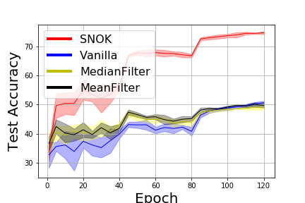
(a) DenseNet-CIFAR10

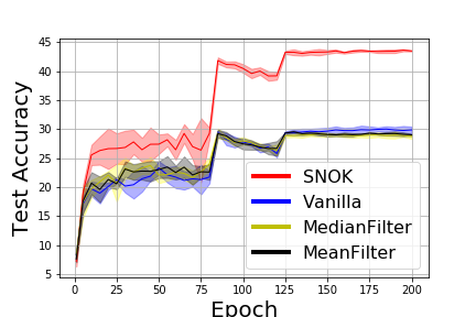
(b) DenseNet-CIFAR100

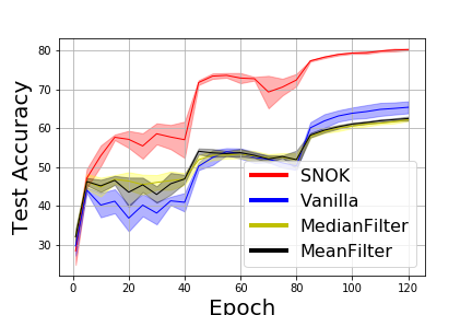
(c) ResNet34-CIFAR10

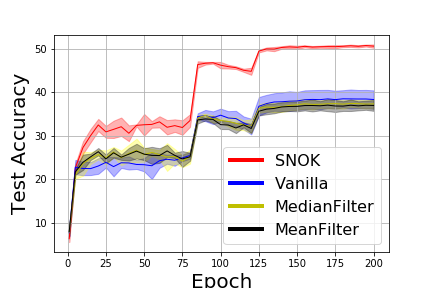
(d) ResNet34-CIFAR100

Figure 1: Mean test accuracy $\pm$ std over 5 independent runs on CIFAR10/CIFAR100 dataset under FGSM adversarial attack for DenseNet and ResNet backbone.

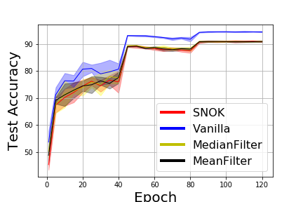
(a) CIFAR10-Clean

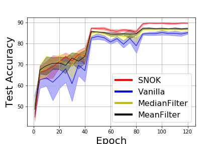
(b) CIFAR10-Gaussian-0.1

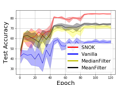
(c) CIFAR10-Gaussian-0.2

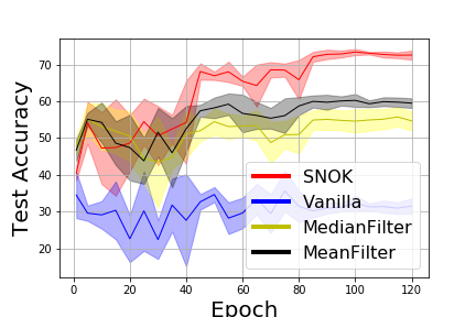
(d) CIFAR10-Gaussian-0.3

(e) CIFAR100-Clean

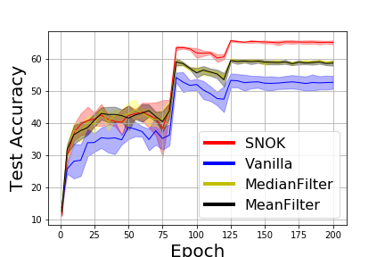
(f) CIFAR100-Gaussian-0.1

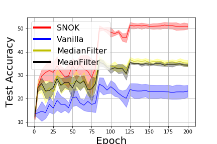
(g) CIFAR100-Gaussian-0.2

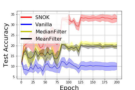
(h) CIFAR100-Gaussian-0.3

Figure 2: Mean test accuracy $\pm$ std over 5 independent runs on DenseNet with Gaussian noise.

We evaluate the performance of our unsupervised SNOK blocks on classification tasks with input noise (Gaussian noise or Laplace noise), and under FGSM adversarial attack [16]. In all the experiments, the input noise is added after input normalization. The standard deviation of input noise is set to $\{0,0.1,0.2,0.3\}$, respectively. We employ both DenseNet-100 [22] and ResNet-34 [19] as backbone. We test the performance of four methods in comparison: (1) Vanilla Backbone, (2) Backbone + Mean Filter, (3) Backbone + Median Filter, (4) Backbone + SNOK. For both Mean Filter and Median Filter cases, we set the filter neighborhood size as $3\times 3$ same as in [38]. For our SNOK case, we plug two SNOK blocks before and after the first learnable Conv2D layer. In all the experiments, CIFAR10 and CIFAR100 datasets [25] are employed for evaluation. All the methods are evaluated over five independent runs with seeds $\{1,2,3,4,5\}$. During training, we stored the model every five epochs, and reported all evaluation results over all the stored models. It covers the whole training trajectory, which is more informative.

The experimental results of different models under the FGSM attack are shown in Fig. 1. Our SNOK plug-in achieves a significantly higher test accuracy than baselines. The results of classification with Gaussian input noise on DenseNet backbone are shown in Fig. 2. Our SNOK obtains competitive performance on the clean case and increasingly better performance as the std increases. More detailed experimental results are presented in Appendix K.

7 Conclusion and Future Work

We proposed a novel kernel family NOK that broadens the connection between deep neural networks and kernel methods. The architecture of our structured approximated NOK performs monotonic descent updates of implicit regularization problems. We can implicitly choose the regularization problems by employing different activation functions, e.g., ReLU, max pooling, and soft-thresholding. Moreover, by taking advantage of the connection to kernel methods, we show that training regularized NOK at an infinite width regime with functional gradient descent converges to a global minimizer. Furthermore, we establish generalization bounds of our SNOK. We show that increasing the width of SNOK can increase the expressive power to reduce the empirical risk and potentially reduce the generalization bound simultaneously through last-layer feature mutual coherence regularization (i.e., $\mu(\boldsymbol{Y}_{T+1})$). In particular, when the width of SNOK is larger than the number of training data, last-layer orthogonal representation can significantly reduce the generalization bound. Our unsupervised structured approximated NOK block can serve as a simple plug-in of popular backbones for a good generalization against input noise. Extensive experiments on CIFAR10 and CIFAR100 with ResNet and DenseNet backbones show the good generalization of our structured approximated NOK against the Gaussian noise, Laplace noise, and FGSM adversarial attack.

In the future, we will investigate the convergence behavior of training the supervised SNOK with SGD at a finite width regime. More interestingly, we will investigate our SNOK with shared parameter $\boldsymbol{R}$ as recurrent neural network architectures.

Appendix A Proof of Proposition 1

Kernel Property:

Proposition.

For $\forall f(\cdot,\boldsymbol{x}),f(\cdot,\boldsymbol{y})\in\mathcal{F}$ ( $\mathcal{F}=\mathcal{L}_{2}$ or $\mathcal{F}=\overline{\mathcal{L}}_{2}$), define function $k(\boldsymbol{x},\boldsymbol{y})=\mathbb{E}_{\boldsymbol{w}}{[f(\boldsymbol{w},\boldsymbol{x})f(\boldsymbol{w},\boldsymbol{y})]}:\mathcal{X}\times\mathcal{X}\to\mathcal{R}$, then $k(\boldsymbol{x},\boldsymbol{y})$ is a bounded kernel, i.e., $k(\boldsymbol{x},\boldsymbol{y})=k(\boldsymbol{y},\boldsymbol{x})<\infty$ and $k(\boldsymbol{x},\boldsymbol{y})$ is positive definite.

Proof.

(i) Symmetric property is straightforward by definition.

(ii) From Cauchy–Schwarz inequality,

$$k(\boldsymbol{x},\boldsymbol{y})=\mathbb{E}_{\boldsymbol{w}}{[f(\boldsymbol{w},\boldsymbol{x})f(\boldsymbol{w},\boldsymbol{y})]}\leq\sqrt{\mathbb{E}_{\boldsymbol{w}}{[f(\boldsymbol{w},\boldsymbol{x})^{2}]}\mathbb{E}_{\boldsymbol{w}}{[f(\boldsymbol{w},\boldsymbol{y})^{2}]}}<\infty$$ (28)

(iii) Positive definite property. For $\forall n\in\mathbb{N}$, $\forall\alpha_{1}\cdots,\alpha_{n}\in\mathcal{R}$ and $\forall\boldsymbol{x}_{1},\cdots,\boldsymbol{x}_{n}\in\mathcal{X}$, we have

$$\sum_{i}{\sum_{j}{\alpha_{i}\alpha_{j}k(\boldsymbol{x}_{i},\boldsymbol{x}_{j})}}=\mathbb{E}_{\boldsymbol{w}}\big{[}\big{(}\sum_{i}\alpha_{i}f(\boldsymbol{w},\boldsymbol{x}_{i})\big{)}^{2}\big{]}\geq 0$$

∎

Appendix B Proof of Theorem 2

Convex $\phi$-regularization:

$$\min_{f\in\mathcal{F}}\frac{1}{2}\|\boldsymbol{x}-\mathbb{E}_{\boldsymbol{w}}[\boldsymbol{w}f(\boldsymbol{w})]\|_{2}^{2}+\mathbb{E}_{\boldsymbol{w}}[\phi_{\lambda}(f(\boldsymbol{w}))]$$ (29)

where $\mathcal{F}=\mathcal{L}_{2}$ or $\mathcal{F}=\overline{\mathcal{L}}_{2}$. And $\mathcal{L}_{2}$ denotes the Gaussian square integrable functional space, i.e., $\mathcal{L}_{2}:=\{f\big{|}\mathbb{E}_{\boldsymbol{w}\sim\mathcal{N}(\boldsymbol{0},\boldsymbol{I}_{d})}[f(\boldsymbol{w})^{2}]<\infty\}$, $\overline{\mathcal{L}}_{2}$ denotes the sphere square integrable functional space, i.e., $\overline{\mathcal{L}}_{2}:=\{f\big{|}\mathbb{E}_{\boldsymbol{w}\sim Uni[\sqrt{d}\mathbb{S}^{d-1}]}[f(\boldsymbol{w})^{2}]<\infty\}$ and $\phi_{\lambda}(\cdot)$ denotes a convex function bounded from below.

Lemma 1.

$\mathbb{E}_{\boldsymbol{w}\sim Uni[\sqrt{d}\mathbb{S}^{d-1}]}[\boldsymbol{w}\boldsymbol{w}^{\top}]=\boldsymbol{I}_{d}$.

Proof.

$$\boldsymbol{I}_{d} =\mathbb{E}_{\boldsymbol{x}\sim\mathcal{N}(\boldsymbol{0},\boldsymbol{I}_{d})}[\boldsymbol{x}\boldsymbol{x}^{\top}]$$

$$=\int\frac{1}{(2\pi)^{\frac{d}{2}}}e^{-\frac{\|\boldsymbol{x}\|_{2}^{2}}{2}}\boldsymbol{x}\boldsymbol{x}^{\top}\,d\boldsymbol{x}$$

$$=\int_{0}^{\infty}{\int_{\mathbb{S}^{d-1}}{\frac{2\pi^{\frac{d}{2}}}{\Gamma(\frac{d}{2})}r^{d-1}\cdot e^{-\frac{r^{2}}{2}}r^{2}\cdot\frac{1}{(2\pi)^{\frac{d}{2}}}\boldsymbol{v}\boldsymbol{v}^{\top}\,d\sigma(\boldsymbol{v})}\,dr}$$ (30)

$$=\int_{0}^{\infty}{\frac{2\pi^{\frac{d}{2}}}{\Gamma(\frac{d}{2})}r^{d-1}e^{-\frac{r^{2}}{2}}r^{2}\cdot\frac{1}{(2\pi)^{\frac{d}{2}}}\,dr}\int_{\mathbb{S}^{d-1}}{\boldsymbol{v}\boldsymbol{v}^{\top}\,d\sigma(\boldsymbol{v})}$$ (31)

$$=\int_{0}^{\infty}{\frac{r^{d-1}e^{-\frac{r^{2}}{2}}}{2^{\frac{d}{2}-1}\Gamma(\frac{d}{2})}r^{2}\,dr}\int_{\mathbb{S}^{d-1}}{\boldsymbol{v}\boldsymbol{v}^{\top}\,d\sigma(\boldsymbol{v})}$$ (32)

$$=\mathbb{E}_{r\sim\chi(d)}{[r^{2}]}\int_{\mathbb{S}^{d-1}}{\boldsymbol{v}\boldsymbol{v}^{\top}\,d\sigma(\boldsymbol{v})}$$ (33)

$$=d\int_{\mathbb{S}^{d-1}}{\boldsymbol{v}\boldsymbol{v}^{\top}\,d\sigma(\boldsymbol{v})}$$ (34)

$$=\mathbb{E}_{\boldsymbol{w}\sim Uni[\sqrt{d}\mathbb{S}^{d-1}]}[\boldsymbol{w}\boldsymbol{w}^{\top}]$$ (35)

where $\sigma(\cdot)$ denotes the normalized surface measure, $\chi(d)$ denotes the Chi distribution with degree $d$, $\Gamma(\cdot)$ denotes the gamma function. ∎

Lemma 2.

Let $f\in\mathcal{F}$ with $\mathcal{F}=\mathcal{L}_{2}$ or $\mathcal{F}=\overline{\mathcal{L}}_{2}$, then we have

$$\mathbb{E}_{\boldsymbol{w}}[f(\boldsymbol{w})^{2}]-\|\mathbb{E}_{\boldsymbol{w}}[\boldsymbol{w}f(\boldsymbol{w})]\|_{2}^{2}=\mathbb{E}_{\boldsymbol{w}}[\big{(}f(\boldsymbol{w})-\boldsymbol{w}^{\top}\mathbb{E}_{\boldsymbol{w}}[\boldsymbol{w}f(\boldsymbol{w})]\big{)}^{2}]\geq 0$$ (36)

Proof.

Let $w_{i}$ denote the $i^{th}$ component of $\boldsymbol{w}$, from Cauchy–Schwarz inequality, we know that

$$(\mathbb{E}_{\boldsymbol{w}}[{w}_{i}f(\boldsymbol{w})])^{2}\leq\mathbb{E}_{\boldsymbol{w}}[{w}_{i}^{2}]\mathbb{E}_{\boldsymbol{w}}[f(\boldsymbol{w})^{2}]=\mathbb{E}_{\boldsymbol{w}}[f(\boldsymbol{w})^{2}]<\infty$$ (37)

Thus the expectation $\mathbb{E}_{\boldsymbol{w}}[\boldsymbol{w}f(\boldsymbol{w})]$ exits.

Since $\mathbb{E}_{\boldsymbol{w}}[\boldsymbol{w}\boldsymbol{w}^{\top}]=\boldsymbol{I}_{d}$, we have

$$\|\mathbb{E}_{\boldsymbol{w}}[\boldsymbol{w}f(\boldsymbol{w})]\|_{2}^{2} =(\mathbb{E}_{\boldsymbol{w}}[\boldsymbol{w}f(\boldsymbol{w})])^{\top}(\mathbb{E}_{\boldsymbol{w}}[\boldsymbol{w}f(\boldsymbol{w})])$$ (38)

$$=(\mathbb{E}_{\boldsymbol{w}}[\boldsymbol{w}f(\boldsymbol{w})])^{\top}\mathbb{E}_{\boldsymbol{w}}{[\boldsymbol{w}\boldsymbol{w}^{\top}]}(\mathbb{E}_{\boldsymbol{w}}[\boldsymbol{w}f(\boldsymbol{w})])$$ (39)

$$=\mathbb{E}_{\boldsymbol{w}}{[(\boldsymbol{w}^{\top}\mathbb{E}_{\boldsymbol{w}}[\boldsymbol{w}f(\boldsymbol{w})])^{2}]}$$ (40)

It follows that

$$\mathbb{E}_{\boldsymbol{w}}[f(\boldsymbol{w})^{2}]-\|\mathbb{E}_{\boldsymbol{w}}[\boldsymbol{w}f(\boldsymbol{w})]\|_{2}^{2}$$

$$=\mathbb{E}_{\boldsymbol{w}}[f(\boldsymbol{w})^{2}]-2\|\mathbb{E}_{\boldsymbol{w}}[\boldsymbol{w}f(\boldsymbol{w})]\|_{2}^{2}+\|\mathbb{E}_{\boldsymbol{w}}[\boldsymbol{w}f(\boldsymbol{w})]\|_{2}^{2}$$ (41)

$$=\mathbb{E}_{\boldsymbol{w}}[f(\boldsymbol{w})^{2}]-2(\mathbb{E}_{\boldsymbol{w}}[\boldsymbol{w}f(\boldsymbol{w})])^{\top}(\mathbb{E}_{\boldsymbol{w}}[\boldsymbol{w}f(\boldsymbol{w})])+\mathbb{E}_{\boldsymbol{w}}{[(\boldsymbol{w}^{\top}\mathbb{E}_{\boldsymbol{w}}[\boldsymbol{w}f(\boldsymbol{w})])^{2}]}$$ (42)

$$=\mathbb{E}_{\boldsymbol{w}}[f(\boldsymbol{w})^{2}]-2\mathbb{E}_{\boldsymbol{w}}[f(\boldsymbol{w})\boldsymbol{w}^{\top}\mathbb{E}_{\boldsymbol{w}}[\boldsymbol{w}f(\boldsymbol{w})]]+\mathbb{E}_{\boldsymbol{w}}{[(\boldsymbol{w}^{\top}\mathbb{E}_{\boldsymbol{w}}[\boldsymbol{w}f(\boldsymbol{w})])^{2}]}$$ (43)

$$=\mathbb{E}_{\boldsymbol{w}}[\big{(}f(\boldsymbol{w})-\boldsymbol{w}^{\top}\mathbb{E}_{\boldsymbol{w}}[\boldsymbol{w}f(\boldsymbol{w})]\big{)}^{2}]\geq 0$$ (44)

∎

Lemma 3.

Let $f\in\mathcal{F}$ with $\mathcal{F}=\mathcal{L}_{2}$ or $\mathcal{F}=\overline{\mathcal{L}}_{2}$, we have

$$\|\boldsymbol{x}-\mathbb{E}_{\boldsymbol{w}}[\boldsymbol{w}f(\boldsymbol{w})]\|_{2}^{2}=\mathbb{E}_{\boldsymbol{w}}{[(\boldsymbol{w}^{\top}(\boldsymbol{x}-\mathbb{E}_{\boldsymbol{w}}[\boldsymbol{w}f(\boldsymbol{w})]))^{2}]}$$ (45)

Proof.

Since $\mathbb{E}_{\boldsymbol{w}}[\boldsymbol{w}\boldsymbol{w}^{\top}]=\boldsymbol{I}_{d}$, we have

$$\|\boldsymbol{x}-\mathbb{E}_{\boldsymbol{w}}[\boldsymbol{w}f(\boldsymbol{w})]\|_{2}^{2} =(\boldsymbol{x}-\mathbb{E}_{\boldsymbol{w}}[\boldsymbol{w}f(\boldsymbol{w})])^{\top}(\boldsymbol{x}-\mathbb{E}_{\boldsymbol{w}}[\boldsymbol{w}f(\boldsymbol{w})])$$ (46)

$$=(\boldsymbol{x}-\mathbb{E}_{\boldsymbol{w}}[\boldsymbol{w}f(\boldsymbol{w})])^{\top}\mathbb{E}_{\boldsymbol{w}}{[\boldsymbol{w}\boldsymbol{w}^{\top}]}(\boldsymbol{x}-\mathbb{E}_{\boldsymbol{w}}[\boldsymbol{w}f(\boldsymbol{w})])$$ (47)

$$=\mathbb{E}_{\boldsymbol{w}}{[(\boldsymbol{w}^{\top}(\boldsymbol{x}-\mathbb{E}_{\boldsymbol{w}}[\boldsymbol{w}f(\boldsymbol{w})]))^{2}]}$$ (48)

∎

Lemma 4.

Denote $L(f):=\frac{1}{2}\|\boldsymbol{x}-\mathbb{E}_{\boldsymbol{w}}[\boldsymbol{w}f(\boldsymbol{w})]\|_{2}^{2}$. For $\forall{f},{g}\in\mathcal{F}$ with $\mathcal{F}=\mathcal{L}_{2}$ or $\mathcal{F}=\overline{\mathcal{L}}_{2}$, we have $L(f)=L(g)+\mathbb{E}_{\boldsymbol{w}}{[\boldsymbol{w}^{\top}(\mathbb{E}_{\boldsymbol{w}}[\boldsymbol{w}g(\boldsymbol{w})]-\boldsymbol{x})\big{(}f(\boldsymbol{w})-g(\boldsymbol{w})\big{)}]}+\frac{1}{2}\|\mathbb{E}_{\boldsymbol{w}}{[\boldsymbol{w}\big{(}f(\boldsymbol{w})-g(\boldsymbol{w})\big{)}]}\|_{2}^{2}$.

Proof.

$$\frac{1}{2}\|\boldsymbol{x}-\mathbb{E}_{\boldsymbol{w}}[\boldsymbol{w}f(\boldsymbol{w})]\|_{2}^{2} =\frac{1}{2}\|\boldsymbol{x}-\mathbb{E}_{\boldsymbol{w}}[\boldsymbol{w}g(\boldsymbol{w})]+\mathbb{E}_{\boldsymbol{w}}[\boldsymbol{w}g(\boldsymbol{w})]-\mathbb{E}_{\boldsymbol{w}}[\boldsymbol{w}f(\boldsymbol{w})]\|_{2}^{2}$$ (49)

$$=\frac{1}{2}\|\boldsymbol{x}-\mathbb{E}_{\boldsymbol{w}}[\boldsymbol{w}g(\boldsymbol{w})]\|_{2}^{2}+\frac{1}{2}\big{\|}\mathbb{E}_{\boldsymbol{w}}[\boldsymbol{w}g(\boldsymbol{w})]-\mathbb{E}_{\boldsymbol{w}}[\boldsymbol{w}f(\boldsymbol{w})]\big{\|}_{2}^{2}$$

$$+\left<\boldsymbol{x}-\mathbb{E}_{\boldsymbol{w}}[\boldsymbol{w}g(\boldsymbol{w})],\mathbb{E}_{\boldsymbol{w}}[\boldsymbol{w}g(\boldsymbol{w})]-\mathbb{E}_{\boldsymbol{w}}[\boldsymbol{w}f(\boldsymbol{w})]\right>$$ (50)

The inner product term can be rewritten as

$$\left<\boldsymbol{x}-\mathbb{E}_{\boldsymbol{w}}[\boldsymbol{w}g(\boldsymbol{w})],\mathbb{E}_{\boldsymbol{w}}[\boldsymbol{w}g(\boldsymbol{w})]-\mathbb{E}_{\boldsymbol{w}}[\boldsymbol{w}f(\boldsymbol{w})]\right> =(\boldsymbol{x}-\mathbb{E}_{\boldsymbol{w}}[\boldsymbol{w}g(\boldsymbol{w})])^{\top}\mathbb{E}_{\boldsymbol{w}}[\boldsymbol{w}\big{(}g(\boldsymbol{w})-f(\boldsymbol{w})\big{)}]$$ (51)

$$=\mathbb{E}_{\boldsymbol{w}}[(\boldsymbol{x}-\mathbb{E}_{\boldsymbol{w}}[\boldsymbol{w}g(\boldsymbol{w})])^{\top}\boldsymbol{w}\big{(}g(\boldsymbol{w})-f(\boldsymbol{w})\big{)}]$$ (52)

It follows that

$$\frac{1}{2}\|\boldsymbol{x}-\mathbb{E}_{\boldsymbol{w}}[\boldsymbol{w}f(\boldsymbol{w})]\|_{2}^{2} =\frac{1}{2}\|\boldsymbol{x}-\mathbb{E}_{\boldsymbol{w}}[\boldsymbol{w}g(\boldsymbol{w})]\|_{2}^{2}+\frac{1}{2}\big{\|}\mathbb{E}_{\boldsymbol{w}}[\boldsymbol{w}\big{(}g(\boldsymbol{w})-f(\boldsymbol{w})\big{)}]\big{\|}_{2}^{2}$$

$$+\mathbb{E}_{\boldsymbol{w}}{[\boldsymbol{w}^{\top}(\mathbb{E}_{\boldsymbol{w}}[\boldsymbol{w}g(\boldsymbol{w})]-\boldsymbol{x})\big{(}f(\boldsymbol{w})-g(\boldsymbol{w})\big{)}]}$$ (53)

∎

Lemma 5.

For $\forall f_{t},f_{t+1},f^{*}\in\mathcal{F}$ with $\mathcal{F}=\mathcal{L}_{2}$ or $\mathcal{F}=\overline{\mathcal{L}}_{2}$, we have

$$L(f_{t+1})\! =\!L(f^{*})\!\!+\!\!\mathbb{E}_{\boldsymbol{w}}{[\boldsymbol{w}^{\top}(\mathbb{E}_{\boldsymbol{w}}[\boldsymbol{w}f_{t}(\boldsymbol{w})]\!\!-\!\!\boldsymbol{x})\big{(}f_{t+1}(\boldsymbol{w})\!-\!f^{*}(\boldsymbol{w})\big{)}]}\!\!+\!\!\frac{1}{2}\|\mathbb{E}_{\boldsymbol{w}}{[\boldsymbol{w}\big{(}f_{t+1}(\boldsymbol{w})\!-\!f_{t}(\boldsymbol{w})\big{)}]}\|_{2}^{2}$$

$$-\frac{1}{2}\|\mathbb{E}_{\boldsymbol{w}}{[\boldsymbol{w}\big{(}f_{t}(\boldsymbol{w})\!-\!f^{*}(\boldsymbol{w})\big{)}]}\|_{2}^{2}$$ (54)

Proof.

From Lemma 4, we know that

$$L(f_{t\!+\!1})=L(f_{t})+\mathbb{E}_{\boldsymbol{w}}{[\boldsymbol{w}^{\top}(\mathbb{E}_{\boldsymbol{w}}[\boldsymbol{w}f_{t}(\boldsymbol{w})]-\boldsymbol{x})\big{(}f_{t\!+\!1}(\boldsymbol{w})-f_{t}(\boldsymbol{w})\big{)}]}+\frac{1}{2}\|\mathbb{E}_{\boldsymbol{w}}{[\boldsymbol{w}\big{(}f_{t\!+\!1}(\boldsymbol{w})-f_{t}(\boldsymbol{w})\big{)}]}\|_{2}^{2}$$ (55)

$$L(f^{*})=L(f_{t})+\mathbb{E}_{\boldsymbol{w}}{[\boldsymbol{w}^{\top}(\mathbb{E}_{\boldsymbol{w}}[\boldsymbol{w}f_{t}(\boldsymbol{w})]-\boldsymbol{x})\big{(}f^{*}(\boldsymbol{w})-f_{t}(\boldsymbol{w})\big{)}]}+\frac{1}{2}\|\mathbb{E}_{\boldsymbol{w}}{[\boldsymbol{w}\big{(}f^{*}(\boldsymbol{w})-f_{t}(\boldsymbol{w})\big{)}]}\|_{2}^{2}$$ (56)

Plug $L(f_{t})$ into Eq.(55), we can obtain that

$$L(f_{t+1})\! =\!L(f^{*})\!\!-\!\!\mathbb{E}_{\boldsymbol{w}}{[\boldsymbol{w}^{\top}(\mathbb{E}_{\boldsymbol{w}}[\boldsymbol{w}f_{t}(\boldsymbol{w})]\!\!-\!\!\boldsymbol{x})\big{(}f^{*}(\boldsymbol{w})\!-\!f_{t}(\boldsymbol{w})\big{)}]}-\frac{1}{2}\|\mathbb{E}_{\boldsymbol{w}}{[\boldsymbol{w}\big{(}f^{*}(\boldsymbol{w})\!-\!f_{t}(\boldsymbol{w})\big{)}]}\|_{2}^{2}$$

$$+\!\!\mathbb{E}_{\boldsymbol{w}}{[\boldsymbol{w}^{\top}(\mathbb{E}_{\boldsymbol{w}}[\boldsymbol{w}f_{t}(\boldsymbol{w})]\!\!-\!\!\boldsymbol{x})\big{(}f_{t+1}(\boldsymbol{w})\!-\!f_{t}(\boldsymbol{w})\big{)}]}\!+\!\frac{1}{2}\|\mathbb{E}_{\boldsymbol{w}}{[\boldsymbol{w}\big{(}f_{t+1}(\boldsymbol{w})\!-\!f_{t}(\boldsymbol{w})\big{)}]}\|_{2}^{2}$$ (57)

$$=\!L(f^{*})\!\!+\!\!\mathbb{E}_{\boldsymbol{w}}{[\boldsymbol{w}^{\top}(\mathbb{E}_{\boldsymbol{w}}[\boldsymbol{w}f_{t}(\boldsymbol{w})]\!\!-\!\!\boldsymbol{x})\big{(}f_{t+1}(\boldsymbol{w})\!-\!f^{*}(\boldsymbol{w})\big{)}]}\!\!+\!\!\frac{1}{2}\|\mathbb{E}_{\boldsymbol{w}}{[\boldsymbol{w}\big{(}f_{t+1}(\boldsymbol{w})\!-\!f_{t}(\boldsymbol{w})\big{)}]}\|_{2}^{2}$$

$$-\frac{1}{2}\|\mathbb{E}_{\boldsymbol{w}}{[\boldsymbol{w}\big{(}f_{t}(\boldsymbol{w})\!-\!f^{*}(\boldsymbol{w})\big{)}]}\|_{2}^{2}$$ (58)

∎

Lemma 6.

For a convex function $\phi_{\lambda}(\cdot)$, denote $h(\cdot)$ as the proximal operator of $\phi_{\lambda}(\cdot)$, i.e., $h(z)=\operatorname*{arg\,min}_{x}{\frac{1}{2}(x-z)^{2}+\phi_{\lambda}(x)}$, let $f_{t+1}=h\circ g_{t+1}\in\mathcal{F}$ with $\mathcal{F}=\mathcal{L}_{2}$ or $\mathcal{F}=\overline{\mathcal{L}}_{2}$, then for $\forall f^{*}\in\mathcal{F}$, we have

$$\mathbb{E}_{\boldsymbol{w}}[\phi_{\lambda}(f_{t+1}(\boldsymbol{w}))]\leq\mathbb{E}_{\boldsymbol{w}}[\phi_{\lambda}(f^{*}(\boldsymbol{w}))]-\mathbb{E}_{\boldsymbol{w}}{[\big{(}g_{t+1}(\boldsymbol{w})-f_{t+1}(\boldsymbol{w})\big{)}\big{(}f^{*}(\boldsymbol{w})-f_{t+1}(\boldsymbol{w})\big{)}]}$$ (59)

Proof.

Since $\phi_{\lambda}(\cdot)$ is convex function and $f_{t+1}(\boldsymbol{w})=\operatorname*{arg\,min}_{{x}}\phi_{\lambda}({x})+\frac{1}{2}\|x-{g}_{t+1}(\boldsymbol{w})\|_{2}^{2}$, we have

$${0}\in\partial\phi_{\lambda}(f_{t+1}(\boldsymbol{w}))+(f_{t+1}(\boldsymbol{w})-g_{t+1}(\boldsymbol{w}))\implies(g_{t+1}(\boldsymbol{w})-f_{t+1}(\boldsymbol{w}))\in\partial\phi_{\lambda}({f}_{t+1}(\boldsymbol{w}))$$ (60)

From the definition of subgradient and convex function $\phi_{\lambda}(\cdot)$, we have

$$\phi_{\lambda}(f_{t+1}(\boldsymbol{w}))\leq\phi_{\lambda}(f^{*}(\boldsymbol{w}))-(g_{t+1}(\boldsymbol{w})-f_{t+1}(\boldsymbol{w}))(f^{*}(\boldsymbol{w})-f_{t+1}(\boldsymbol{w}))$$ (61)

It follows that

$$\mathbb{E}_{\boldsymbol{w}}[\phi_{\lambda}(f_{t+1}(\boldsymbol{w}))]\leq\mathbb{E}_{\boldsymbol{w}}[\phi_{\lambda}(f^{*}(\boldsymbol{w}))]-\mathbb{E}_{\boldsymbol{w}}{[\big{(}g_{t+1}(\boldsymbol{w})-f_{t+1}(\boldsymbol{w})\big{)}\big{(}f^{*}(\boldsymbol{w})-f_{t+1}(\boldsymbol{w})\big{)}]}$$ (62)

∎

Lemma 7.

Denote $h(\cdot)$ as the proximal operator of $\phi_{\lambda}(\cdot)$. Suppose $|h(x)|\leq c|x|$ (or $|h(x)|\leq c$) , $0<c<\infty$ . Given a bouned $\boldsymbol{x}\in\mathcal{R}^{d}$, set function $g_{t+1}(\boldsymbol{w})=\boldsymbol{w}^{\top}\boldsymbol{x}+f_{t}(\boldsymbol{w})-\boldsymbol{w}^{\top}\mathbb{E}_{\boldsymbol{w}}{[\boldsymbol{w}f_{t}(\boldsymbol{w})]}$ with $f_{t}\in\mathcal{L}_{2}$ and $\boldsymbol{w}\sim\mathcal{N}(\boldsymbol{0},\boldsymbol{I}_{d})$ (or $f_{t}\in\overline{\mathcal{L}}_{2}$ and $\boldsymbol{w}\sim Uni[\sqrt{d}\mathbb{S}^{d-1}]$). Set $f_{t+1}=h\circ g_{t+1}$, then, we know $f_{t+1}\in\mathcal{F}$ with $\mathcal{F}=\mathcal{L}_{2}$ or $\mathcal{F}=\overline{\mathcal{L}}_{2}$,respectively.

Proof.

Case $|h(x)|\leq c,\;0<c<\infty$: It is straightforward to know $\mathbb{E}_{\boldsymbol{w}}{[h(g_{t+1}(\boldsymbol{w}))^{2}]}\leq c^{2}<\infty$, thus $f_{t+1}\in\mathcal{F}$.

Case $|h(x)|\leq c|x|,\;0<c<\infty$: Since $|h(x)|\leq c|x|$, we know that

$$h(g_{t+1}(\boldsymbol{w}))^{2}\leq c^{2}g_{t+1}(\boldsymbol{w})^{2} =c^{2}\big{(}\boldsymbol{w}^{\top}\boldsymbol{x}+f_{t}(\boldsymbol{w})-\boldsymbol{w}^{\top}\mathbb{E}_{\boldsymbol{w}}{[\boldsymbol{w}f_{t}(\boldsymbol{w})]}\big{)}^{2}$$ (63)

$$\leq 2c^{2}(\boldsymbol{w}^{\top}(\boldsymbol{x}-\mathbb{E}_{\boldsymbol{w}}{[\boldsymbol{w}f_{t}(\boldsymbol{w})]}))^{2}+2c^{2}f_{t}(\boldsymbol{w})^{2}$$ (64)

It follows that

$$\mathbb{E}_{\boldsymbol{w}}{[h(g_{t+1}(\boldsymbol{w}))^{2}]} \leq c^{2}\mathbb{E}_{\boldsymbol{w}}{[\big{(}\boldsymbol{w}^{\top}\boldsymbol{x}+f_{t}(\boldsymbol{w})-\boldsymbol{w}^{\top}\mathbb{E}_{\boldsymbol{w}}{[\boldsymbol{w}f_{t}(\boldsymbol{w})]}\big{)}^{2}]}$$ (65)

$$\leq 2c^{2}\mathbb{E}_{\boldsymbol{w}}{[(\boldsymbol{w}^{\top}(\boldsymbol{x}-\mathbb{E}_{\boldsymbol{w}}{[\boldsymbol{w}f_{t}(\boldsymbol{w})]}))^{2}]}+2c^{2}\mathbb{E}_{\boldsymbol{w}}{[f_{t}(\boldsymbol{w})^{2}]}$$ (66)

$$=2c^{2}\|\boldsymbol{x}-\mathbb{E}_{\boldsymbol{w}}{[\boldsymbol{w}f_{t}(\boldsymbol{w})]}\|_{2}^{2}+2c^{2}\mathbb{E}_{\boldsymbol{w}}{[f_{t}(\boldsymbol{w})^{2}]}$$ (67)

$$\leq 4c^{2}\|\boldsymbol{x}\|_{2}^{2}+4c^{2}\|\mathbb{E}_{\boldsymbol{w}}[\boldsymbol{w}f_{t}(\boldsymbol{w})]\|_{2}^{2}+2c^{2}\mathbb{E}_{\boldsymbol{w}}{[f_{t}(\boldsymbol{w})^{2}]}$$ (68)

From Lemma 2, we know $\|\mathbb{E}_{\boldsymbol{w}}[\boldsymbol{w}f_{t}(\boldsymbol{w})]\|_{2}^{2}\leq\mathbb{E}_{\boldsymbol{w}}{[f_{t}(\boldsymbol{w})^{2}]}$ is bounded, together with $\|\boldsymbol{x}\|_{2}<\infty$,it follows that $\mathbb{E}_{\boldsymbol{w}}{[f_{t+1}(\boldsymbol{w}))^{2}]}=\mathbb{E}_{\boldsymbol{w}}{[h(g_{t+1}(\boldsymbol{w}))^{2}]}<\infty$. Thus, $f_{t+1}\in\mathcal{F}$.

∎

Lemma 8.

For a convex function $\phi_{\lambda}(\cdot)$, denote $h(\cdot)$ as the proximal operator of $\phi_{\lambda}(\cdot)$, i.e., $h(z)=\operatorname*{arg\,min}_{x}{\frac{1}{2}(x-z)^{2}+\phi_{\lambda}(x)}$. Suppose $|h(x)|\leq c|x|$ (or $|h(x)|\leq c$), $0<c<\infty$ (e.g., soft thresholding function). Given a bouned $\boldsymbol{x}\in\mathcal{R}^{d}$, set function $g_{t+1}(\boldsymbol{w})=\boldsymbol{w}^{\top}\boldsymbol{x}+f_{t}(\boldsymbol{w})-\boldsymbol{w}^{\top}\mathbb{E}_{\boldsymbol{w}}{[\boldsymbol{w}f_{t}(\boldsymbol{w})]}$ with $f_{t}\in\mathcal{L}_{2}$ and $\boldsymbol{w}\sim\mathcal{N}(\boldsymbol{0},\boldsymbol{I}_{d})$ (or $f_{t}\in\overline{\mathcal{L}}_{2}$ and $\boldsymbol{w}\sim Uni[\sqrt{d}\mathbb{S}^{d-1}]$). Set $f_{t+1}=h\circ g_{t+1}$. Denote $Q(f)=L(f)+\mathbb{E}_{\boldsymbol{w}}[\phi_{\lambda}(f(\boldsymbol{w}))]$ with $L(f):=\frac{1}{2}\|\boldsymbol{x}-\mathbb{E}_{\boldsymbol{w}}[\boldsymbol{w}f(\boldsymbol{w})]\|_{2}^{2}$, for $\forall f^{*}\in\mathcal{F}$ with $\mathcal{F}=\mathcal{L}_{2}$ or $\mathcal{F}=\overline{\mathcal{L}}_{2}$, we have

$$Q(f_{t+1}) \leq Q(f^{*})\!+\!\frac{1}{2}\mathbb{E}_{\boldsymbol{w}}{[(f_{t}(\boldsymbol{w})\!-\!f^{*}(\boldsymbol{w}))^{2}]}\!-\!\frac{1}{2}\mathbb{E}_{\boldsymbol{w}}{[(f_{t\!+\!1}(\boldsymbol{w})\!-\!f^{*}(\boldsymbol{w}))^{2}]}$$

$$-\frac{1}{2}\|\mathbb{E}_{\boldsymbol{w}}{[\boldsymbol{w}\big{(}f_{t}(\boldsymbol{w})\!-\!f^{*}(\boldsymbol{w})\big{)}]}\|_{2}^{2}$$ (69)

Proof.

From Lemma 5, we know that

$$L(f_{t+1})\! =\!L(f^{*})\!\!+\!\!\mathbb{E}_{\boldsymbol{w}}{[\boldsymbol{w}^{\top}(\mathbb{E}_{\boldsymbol{w}}[\boldsymbol{w}f_{t}(\boldsymbol{w})]\!\!-\!\!\boldsymbol{x})\big{(}f_{t+1}(\boldsymbol{w})\!-\!f^{*}(\boldsymbol{w})\big{)}]}\!\!+\!\!\frac{1}{2}\|\mathbb{E}_{\boldsymbol{w}}{[\boldsymbol{w}\big{(}f_{t+1}(\boldsymbol{w})\!-\!f_{t}(\boldsymbol{w})\big{)}]}\|_{2}^{2}$$

$$-\frac{1}{2}\|\mathbb{E}_{\boldsymbol{w}}{[\boldsymbol{w}\big{(}f_{t}(\boldsymbol{w})\!-\!f^{*}(\boldsymbol{w})\big{)}]}\|_{2}^{2}$$ (70)

Together with Lemma 6, it follows that

$$Q(f_{t+1})$$ (71)

$$\leq\!Q(f^{*})\!\!-\!\!\mathbb{E}_{\boldsymbol{w}}{[\big{(}g_{t\!+\!1}(\boldsymbol{w})\!-\!f_{t+1}(\boldsymbol{w})\big{)}\big{(}f^{*}(\boldsymbol{w})\!\!-\!\!f_{t\!+\!1}(\boldsymbol{w})\big{)}]}\!\!+\!\!\mathbb{E}_{\boldsymbol{w}}{[\boldsymbol{w}^{\top}(\mathbb{E}_{\boldsymbol{w}}[\boldsymbol{w}f_{t}(\boldsymbol{w})]\!\!-\!\!\boldsymbol{x})\big{(}f_{t+1}(\boldsymbol{w})\!\!-\!\!f^{*}(\boldsymbol{w})\big{)}]}$$

$$+\frac{1}{2}\|\mathbb{E}_{\boldsymbol{w}}{[\boldsymbol{w}\big{(}f_{t+1}(\boldsymbol{w})\!-\!f_{t}(\boldsymbol{w})\big{)}]}\|_{2}^{2}-\frac{1}{2}\|\mathbb{E}_{\boldsymbol{w}}{[\boldsymbol{w}\big{(}f_{t}(\boldsymbol{w})\!-\!f^{*}(\boldsymbol{w})\big{)}]}\|_{2}^{2}$$ (72)

$$=\!Q(f^{*})\!\!+\!\!\mathbb{E}_{\boldsymbol{w}}{[\big{(}g_{t\!+\!1}(\boldsymbol{w})\!-\!f_{t+1}(\boldsymbol{w})+\boldsymbol{w}^{\top}(\mathbb{E}_{\boldsymbol{w}}[\boldsymbol{w}f_{t}(\boldsymbol{w})]\!\!-\!\!\boldsymbol{x})\big{)}\big{(}f_{t+1}(\boldsymbol{w})\!\!-\!\!f^{*}(\boldsymbol{w})\big{)}]}$$

$$+\frac{1}{2}\|\mathbb{E}_{\boldsymbol{w}}{[\boldsymbol{w}\big{(}f_{t+1}(\boldsymbol{w})\!-\!f_{t}(\boldsymbol{w})\big{)}]}\|_{2}^{2}-\frac{1}{2}\|\mathbb{E}_{\boldsymbol{w}}{[\boldsymbol{w}\big{(}f_{t}(\boldsymbol{w})\!-\!f^{*}(\boldsymbol{w})\big{)}]}\|_{2}^{2}$$ (73)

$$=\!Q(f^{*})\!\!+\!\!\mathbb{E}_{\boldsymbol{w}}{[\big{(}f_{t}(\boldsymbol{w})\!-\!f_{t+1}(\boldsymbol{w})\big{)}\big{(}f_{t+1}(\boldsymbol{w})\!\!-\!\!f^{*}(\boldsymbol{w})\big{)}]}$$

$$+\frac{1}{2}\|\mathbb{E}_{\boldsymbol{w}}{[\boldsymbol{w}\big{(}f_{t+1}(\boldsymbol{w})\!-\!f_{t}(\boldsymbol{w})\big{)}]}\|_{2}^{2}-\frac{1}{2}\|\mathbb{E}_{\boldsymbol{w}}{[\boldsymbol{w}\big{(}f_{t}(\boldsymbol{w})\!-\!f^{*}(\boldsymbol{w})\big{)}]}\|_{2}^{2}$$ (74)

Note that

$$\mathbb{E}_{\boldsymbol{w}}{[\big{(}f_{t}(\boldsymbol{w})\!-\!f_{t+1}(\boldsymbol{w})\big{)}\big{(}f_{t+1}(\boldsymbol{w})\!\!-\!\!f^{*}(\boldsymbol{w})\big{)}]}$$

$$=\mathbb{E}_{\boldsymbol{w}}{[\big{(}f_{t}(\boldsymbol{w})\!-\!f_{t+1}(\boldsymbol{w})\big{)}\big{(}f_{t+1}(\boldsymbol{w})\!\!-\!\!f_{t}(\boldsymbol{w})\!\!+\!\!f_{t}(\boldsymbol{w})\!\!-\!\!f^{*}(\boldsymbol{w})\big{)}]}$$ (75)

$$=\mathbb{E}_{\boldsymbol{w}}{[\big{(}f_{t}(\boldsymbol{w})\!-\!f_{t+1}(\boldsymbol{w})\big{)}\big{(}f_{t}(\boldsymbol{w})\!\!-\!\!f^{*}(\boldsymbol{w})\big{)}]}-\mathbb{E}_{\boldsymbol{w}}{[\big{(}f_{t}(\boldsymbol{w})\!-\!f_{t+1}(\boldsymbol{w})\big{)}^{2}]}$$ (76)

Also note that $ab=\frac{a^{2}+b^{2}-(a-b)^{2}}{2}$, it follows that

$$\big{(}f_{t}(\boldsymbol{w})\!-\!f_{t+1}(\boldsymbol{w})\big{)}\big{(}f_{t}(\boldsymbol{w})\!-\!f^{*}(\boldsymbol{w})\big{)}=\frac{(f_{t}(\boldsymbol{w})\!-\!f_{t+1}(\boldsymbol{w}))^{2}+(f_{t}(\boldsymbol{w})\!-\!f^{*}(\boldsymbol{w}))^{2}\!-\!(f_{t\!+\!1}(\boldsymbol{w})\!-\!f^{*}(\boldsymbol{w}))^{2}}{2}$$ (77)

It follows that

$$\mathbb{E}_{\boldsymbol{w}}{[\big{(}f_{t}(\boldsymbol{w})\!-\!f_{t+1}(\boldsymbol{w})\big{)}\big{(}f_{t+1}(\boldsymbol{w})\!\!-\!\!f^{*}(\boldsymbol{w})\big{)}]}$$

$$=\frac{1}{2}\mathbb{E}_{\boldsymbol{w}}{[(f_{t}(\boldsymbol{w})\!-\!f^{*}(\boldsymbol{w}))^{2}]}-\frac{1}{2}\mathbb{E}_{\boldsymbol{w}}{[(f_{t\!+\!1}(\boldsymbol{w})\!-\!f^{*}(\boldsymbol{w}))^{2}]}-\frac{1}{2}\mathbb{E}_{\boldsymbol{w}}{[(f_{t\!+\!1}(\boldsymbol{w})\!-\!f_{t}(\boldsymbol{w}))^{2}]}$$ (78)

Plug Eq.(78) into Eq.(74), we can obtain that

$$Q(f_{t+1}) \leq Q(f^{*})+\frac{1}{2}\mathbb{E}_{\boldsymbol{w}}{[(f_{t}(\boldsymbol{w})\!-\!f^{*}(\boldsymbol{w}))^{2}]}-\frac{1}{2}\mathbb{E}_{\boldsymbol{w}}{[(f_{t\!+\!1}(\boldsymbol{w})\!-\!f^{*}(\boldsymbol{w}))^{2}]}-\frac{1}{2}\mathbb{E}_{\boldsymbol{w}}{[(f_{t\!+\!1}(\boldsymbol{w})\!-\!f_{t}(\boldsymbol{w}))^{2}]}$$

$$+\frac{1}{2}\|\mathbb{E}_{\boldsymbol{w}}{[\boldsymbol{w}\big{(}f_{t+1}(\boldsymbol{w})\!-\!f_{t}(\boldsymbol{w})\big{)}]}\|_{2}^{2}-\frac{1}{2}\|\mathbb{E}_{\boldsymbol{w}}{[\boldsymbol{w}\big{(}f_{t}(\boldsymbol{w})\!-\!f^{*}(\boldsymbol{w})\big{)}]}\|_{2}^{2}$$ (79)

From Lemma 2, we know $\|\mathbb{E}_{\boldsymbol{w}}{[\boldsymbol{w}\big{(}f_{t+1}(\boldsymbol{w})\!-\!f_{t}(\boldsymbol{w})\big{)}]}\|_{2}^{2}\leq\mathbb{E}_{\boldsymbol{w}}{[(f_{t\!+\!1}(\boldsymbol{w})\!-\!f_{t}(\boldsymbol{w}))^{2}]}$. It follows that

$$Q(f_{t+1}) \leq Q(f^{*})\!+\!\frac{1}{2}\mathbb{E}_{\boldsymbol{w}}{[(f_{t}(\boldsymbol{w})\!-\!f^{*}(\boldsymbol{w}))^{2}]}\!-\!\frac{1}{2}\mathbb{E}_{\boldsymbol{w}}{[(f_{t\!+\!1}(\boldsymbol{w})\!-\!f^{*}(\boldsymbol{w}))^{2}]}$$ (80)

$$-\frac{1}{2}\|\mathbb{E}_{\boldsymbol{w}}{[\boldsymbol{w}\big{(}f_{t}(\boldsymbol{w})\!-\!f^{*}(\boldsymbol{w})\big{)}]}\|_{2}^{2}$$

∎

Lemma 9.

(Strictly Monotonic Descent (a.s.)) Following the same condition of Lemma 8, we have

$$Q(f_{t+1})\leq Q(f_{t})\!-\!\frac{1}{2}\mathbb{E}_{\boldsymbol{w}}{[(f_{t\!+\!1}(\boldsymbol{w})\!-\!f_{t}(\boldsymbol{w}))^{2}]}$$ (81)

Proof.

It follows directly from Lemma 8 by setting $f^{*}=f_{t}$. ∎

Theorem.

For a convex function $\phi_{\lambda}(\cdot)$, denote $h(\cdot)$ as the proximal operator of $\phi_{\lambda}(\cdot)$, i.e., $h(z)=\operatorname*{arg\,min}_{x}{\frac{1}{2}(x-z)^{2}+\phi_{\lambda}(x)}$. Suppose $|h(x)|\leq c|x|$ (or $|h(x)|\leq c$), $0<c<\infty$. Given a bouned $\boldsymbol{x}\in\mathcal{R}^{d}$, set function $g_{t+1}(\boldsymbol{w})=\boldsymbol{w}^{\top}\boldsymbol{x}+f_{t}(\boldsymbol{w})-\boldsymbol{w}^{\top}\mathbb{E}_{\boldsymbol{w}}{[\boldsymbol{w}f_{t}(\boldsymbol{w})]}$ with $\boldsymbol{w}\sim\mathcal{N}(\boldsymbol{0},\boldsymbol{I}_{d})$ (or $\boldsymbol{w}\sim Uni[\sqrt{d}\mathbb{S}^{d-1}]$). Set $f_{t+1}=h\circ g_{t+1}$ and $f_{0}\in\mathcal{F}$ with $\mathcal{F}=\mathcal{L}_{2}$ or $\mathcal{F}=\overline{\mathcal{L}}_{2}$ (e.g., $f_{0}=0$). Denote $Q(f)=L(f)+\mathbb{E}_{\boldsymbol{w}}[\phi_{\lambda}(f(\boldsymbol{w}))]$ with $L(f):=\frac{1}{2}\|\boldsymbol{x}-\mathbb{E}_{\boldsymbol{w}}[\boldsymbol{w}f(\boldsymbol{w})]\|_{2}^{2}$. Denote $f_{*}\in\mathcal{F}$ as an optimal of $Q(\cdot)$, we have

$$T\big{(}Q(f_{T})-Q(f_{*})\big{)} \leq\frac{1}{2}\mathbb{E}_{\boldsymbol{w}}{[(f_{0}(\boldsymbol{w})\!-\!f_{*}(\boldsymbol{w}))^{2}]}\!-\!\frac{1}{2}\mathbb{E}_{\boldsymbol{w}}{[(f_{T}(\boldsymbol{w})\!-\!f_{*}(\boldsymbol{w}))^{2}]}$$

$$-\frac{1}{2}\sum_{t=0}^{T-1}{\|\mathbb{E}_{\boldsymbol{w}}{[\boldsymbol{w}\big{(}f_{t}(\boldsymbol{w})\!-\!f_{*}(\boldsymbol{w})\big{)}]}\|_{2}^{2}}-\frac{1}{2}\sum_{t=0}^{T-1}{{(t+1)\mathbb{E}_{\boldsymbol{w}}{[(f_{t\!+\!1}(\boldsymbol{w})\!-\!f_{t}(\boldsymbol{w}))^{2}]}}}$$ (82)

Proof.

From Lemma 8, by setting $f^{*}=f_{*}$, we can obtain that

$$Q(f_{t+1}) \leq Q(f_{*})\!+\!\frac{1}{2}\mathbb{E}_{\boldsymbol{w}}{[(f_{t}(\boldsymbol{w})\!-\!f_{*}(\boldsymbol{w}))^{2}]}\!-\!\frac{1}{2}\mathbb{E}_{\boldsymbol{w}}{[(f_{t\!+\!1}(\boldsymbol{w})\!-\!f_{*}(\boldsymbol{w}))^{2}]}$$

$$-\frac{1}{2}\|\mathbb{E}_{\boldsymbol{w}}{[\boldsymbol{w}\big{(}f_{t}(\boldsymbol{w})\!-\!f_{*}(\boldsymbol{w})\big{)}]}\|_{2}^{2}$$ (83)

Telescope the inequality (B) from $t=0$ to $t=T-1$, we can obtain that

$$\sum_{t=0}^{T-1}{Q(f_{t+1})}-TQ(f_{*}) \leq\frac{1}{2}\mathbb{E}_{\boldsymbol{w}}{[(f_{0}(\boldsymbol{w})\!-\!f_{*}(\boldsymbol{w}))^{2}]}\!-\!\frac{1}{2}\mathbb{E}_{\boldsymbol{w}}{[(f_{T}(\boldsymbol{w})\!-\!f_{*}(\boldsymbol{w}))^{2}]}$$

$$-\frac{1}{2}\sum_{t=0}^{T-1}{\|\mathbb{E}_{\boldsymbol{w}}{[\boldsymbol{w}\big{(}f_{t}(\boldsymbol{w})\!-\!f_{*}(\boldsymbol{w})\big{)}]}\|_{2}^{2}}$$ (84)

In addition, from Lemma 9, we can obtain that

$$Q(f_{T})\leq Q(f_{t})-\frac{1}{2}\sum_{i=t}^{T-1}{\mathbb{E}_{\boldsymbol{w}}{[(f_{i\!+\!1}(\boldsymbol{w})\!-\!f_{i}(\boldsymbol{w}))^{2}]}}$$ (85)

It follows that

$$TQ(f_{T})-TQ(f_{*}) \leq\sum_{t=0}^{T-1}{Q(f_{t+1})}-TQ(f_{*})-\frac{1}{2}\sum_{t=0}^{T-1}{\sum_{i=t}^{T-1}{\mathbb{E}_{\boldsymbol{w}}{[(f_{i\!+\!1}(\boldsymbol{w})\!-\!f_{i}(\boldsymbol{w}))^{2}]}}}$$ (86)

$$=\sum_{t=0}^{T-1}{Q(f_{t+1})}-TQ(f_{*})-\frac{1}{2}\sum_{t=0}^{T-1}{{(t+1)\mathbb{E}_{\boldsymbol{w}}{[(f_{t\!+\!1}(\boldsymbol{w})\!-\!f_{t}(\boldsymbol{w}))^{2}]}}}$$ (87)

Plug inequality (B) into inequality (87), we can obtain that

$$TQ(f_{T})-TQ(f_{*}) \leq\frac{1}{2}\mathbb{E}_{\boldsymbol{w}}{[(f_{0}(\boldsymbol{w})\!-\!f_{*}(\boldsymbol{w}))^{2}]}\!-\!\frac{1}{2}\mathbb{E}_{\boldsymbol{w}}{[(f_{T}(\boldsymbol{w})\!-\!f_{*}(\boldsymbol{w}))^{2}]}$$

$$-\frac{1}{2}\sum_{t=0}^{T-1}{\|\mathbb{E}_{\boldsymbol{w}}{[\boldsymbol{w}\big{(}f_{t}(\boldsymbol{w})\!-\!f_{*}(\boldsymbol{w})\big{)}]}\|_{2}^{2}}-\frac{1}{2}\sum_{t=0}^{T-1}{{(t+1)\mathbb{E}_{\boldsymbol{w}}{[(f_{t\!+\!1}(\boldsymbol{w})\!-\!f_{t}(\boldsymbol{w}))^{2}]}}}$$ (88)

∎

Appendix C Proof of Theorem 1

Non-convex $\phi$-regularization:

Theorem.

For a (non-convex) regularization function $\phi_{\lambda}(\cdot)$, denote $h(\cdot)$ as the proximal operator of $\phi_{\lambda}(\cdot)$, i.e., $h(z)=\operatorname*{arg\,min}_{x}{\frac{1}{2}(x-z)^{2}+\phi_{\lambda}(x)}$. Suppose $|h(x)|\leq c|x|$ (or $|h(x)|\leq c$), $0<c<\infty$ (e.g., hard thresholding function). Given a bouned $\boldsymbol{x}\in\mathcal{R}^{d}$, set function $g_{t+1}(\boldsymbol{w})=\boldsymbol{w}^{\top}\boldsymbol{x}+f_{t}(\boldsymbol{w})-\boldsymbol{w}^{\top}\mathbb{E}_{\boldsymbol{w}}{[\boldsymbol{w}f_{t}(\boldsymbol{w})]}$ with $f_{t}\in\mathcal{L}_{2}$ and $\boldsymbol{w}\sim\mathcal{N}(\boldsymbol{0},\boldsymbol{I}_{d})$ (or $f_{t}\in\overline{\mathcal{L}}_{2}$, $\boldsymbol{w}\sim Uni[\sqrt{d}\mathbb{S}^{d-1}]$). Set $f_{t+1}=h\circ g_{t+1}$. Denote $Q(f)=L(f)+\mathbb{E}_{\boldsymbol{w}}[\phi_{\lambda}(f(\boldsymbol{w}))]$ with $L(f):=\frac{1}{2}\|\boldsymbol{x}-\mathbb{E}_{\boldsymbol{w}}[\boldsymbol{w}f(\boldsymbol{w})]\|_{2}^{2}$, we have

$$Q(f_{t\!+\!1})\! \leq\!Q(f_{t})-\frac{1}{2}\mathbb{E}_{\boldsymbol{w}}[\left.(f_{t\!+\!1}(\boldsymbol{w})\!-\!f_{t}(\boldsymbol{w})-\boldsymbol{w}^{\top}\mathbb{E}_{\boldsymbol{w}}[\boldsymbol{w}(f_{t\!+\!1}(\boldsymbol{w})\!-\!f_{t}(\boldsymbol{w}))]\right.)^{2}]\leq Q(f_{t})$$ (89)

Proof.

From Lemma 4, we know that

$$L(f_{t\!+\!1})\!=\!L(f_{t})+\mathbb{E}_{\boldsymbol{w}}{[\boldsymbol{w}^{\top}(\mathbb{E}_{\boldsymbol{w}}[\boldsymbol{w}f_{t}(\boldsymbol{w})]\!-\!\boldsymbol{x})\big{(}f_{t\!+\!1}(\boldsymbol{w})\!-\!f_{t}(\boldsymbol{w})\big{)}]}+\frac{1}{2}\|\mathbb{E}_{\boldsymbol{w}}{[\boldsymbol{w}\big{(}f_{t\!+\!1}(\boldsymbol{w})\!-\!f_{t}(\boldsymbol{w})\big{)}]}\|_{2}^{2}$$ (90)

Let $g_{t+1}(\boldsymbol{w})=\boldsymbol{w}^{\top}\boldsymbol{x}+f_{t}(\boldsymbol{w})-\boldsymbol{w}^{\top}\mathbb{E}_{\boldsymbol{w}}{[\boldsymbol{w}f_{t}(\boldsymbol{w})]}$, together with Eq.(90), we can obtain that

$$L(f_{t\!+\!1})\!=\!L(f_{t})+\mathbb{E}_{\boldsymbol{w}}{[\big{(}f_{t}(\boldsymbol{w})-g_{t+1}(\boldsymbol{w})\big{)}\big{(}f_{t\!+\!1}(\boldsymbol{w})\!-\!f_{t}(\boldsymbol{w})\big{)}]}+\frac{1}{2}\|\mathbb{E}_{\boldsymbol{w}}{[\boldsymbol{w}\big{(}f_{t\!+\!1}(\boldsymbol{w})\!-\!f_{t}(\boldsymbol{w})\big{)}]}\|_{2}^{2}$$ (91)

Note that $ab=\frac{(a+b)^{2}-a^{2}-b^{2}}{2}$, it follows that

$$\big{(}f_{t}(\boldsymbol{w})\!-\!g_{t\!+\!1}(\boldsymbol{w})\big{)}\big{(}f_{t\!+\!1}(\boldsymbol{w})\!-\!f_{t}(\boldsymbol{w})\big{)}\!=\!\frac{\big{(}f_{t\!+\!1}(\boldsymbol{w})\!-\!g_{t\!+\!1}(\boldsymbol{w})\big{)}^{2}\!\!-\!\!\big{(}f_{t}(\boldsymbol{w})\!-\!g_{t\!+\!1}(\boldsymbol{w})\big{)}^{2}\!\!-\!\!\big{(}f_{t\!+\!1}(\boldsymbol{w})\!-\!f_{t}(\boldsymbol{w})\big{)}^{2}}{2}$$ (92)

Since $f_{t+1}=h\circ g_{t+1}$ is the solution of the proximal problem,
i.e., $f_{t+1}(\boldsymbol{w})=\operatorname*{arg\,min}_{x}{\frac{(x-g_{t+1}(\boldsymbol{w}))^{2}}{2}+\phi_{\lambda}(x)}$, we know that

$$\frac{\big{(}f_{t\!+\!1}(\boldsymbol{w})\!-\!g_{t\!+\!1}(\boldsymbol{w})\big{)}^{2}}{2}-\frac{\big{(}f_{t}(\boldsymbol{w})\!-\!g_{t\!+\!1}(\boldsymbol{w})\big{)}^{2}}{2}\leq\phi_{\lambda}(f_{t}(\boldsymbol{w}))-\phi_{\lambda}(f_{t\!+\!1}(\boldsymbol{w}))$$ (93)

It follows that

$$\mathbb{E}_{\boldsymbol{w}}{[\big{(}f_{t}(\boldsymbol{w})-g_{t+1}(\boldsymbol{w})\big{)}\big{(}f_{t\!+\!1}(\boldsymbol{w})\!-\!f_{t}(\boldsymbol{w})\big{)}]}$$

$$=\mathbb{E}_{\boldsymbol{w}}{\left.[\frac{\big{(}f_{t\!+\!1}(\boldsymbol{w})\!-\!g_{t\!+\!1}(\boldsymbol{w})\big{)}^{2}\!\!-\!\!\big{(}f_{t}(\boldsymbol{w})\!-\!g_{t\!+\!1}(\boldsymbol{w})\big{)}^{2}\!\!-\!\!\big{(}f_{t\!+\!1}(\boldsymbol{w})\!-\!f_{t}(\boldsymbol{w})\big{)}^{2}}{2}\right.]}$$ (94)

$$\leq\mathbb{E}_{\boldsymbol{w}}{[\phi_{\lambda}(f_{t}(\boldsymbol{w}))]}-\mathbb{E}_{\boldsymbol{w}}{[\phi_{\lambda}(f_{t+1}(\boldsymbol{w}))]}-\frac{1}{2}\mathbb{E}_{\boldsymbol{w}}{[\big{(}f_{t\!+\!1}(\boldsymbol{w})\!-\!f_{t}(\boldsymbol{w})\big{)}^{2}]}$$ (95)

Plug inequality (95) into Eq.(91), we can achieve that

$$L(f_{t\!+\!1})+\mathbb{E}_{\boldsymbol{w}}{[\phi_{\lambda}(f_{t+1}(\boldsymbol{w}))]}\! \leq\!L(f_{t})+\mathbb{E}_{\boldsymbol{w}}{[\phi_{\lambda}(f_{t}(\boldsymbol{w}))]}-\frac{1}{2}\mathbb{E}_{\boldsymbol{w}}{[\big{(}f_{t\!+\!1}(\boldsymbol{w})\!-\!f_{t}(\boldsymbol{w})\big{)}^{2}]}$$

$$+\frac{1}{2}\|\mathbb{E}_{\boldsymbol{w}}{[\boldsymbol{w}\big{(}f_{t\!+\!1}(\boldsymbol{w})\!-\!f_{t}(\boldsymbol{w})\big{)}]}\|_{2}^{2}$$ (96)

From Lemma 2, we know that

$$\mathbb{E}_{\boldsymbol{w}}{[\big{(}f_{t\!+\!1}(\boldsymbol{w})\!-\!f_{t}(\boldsymbol{w})\big{)}^{2}]}-\|\mathbb{E}_{\boldsymbol{w}}{[\boldsymbol{w}\big{(}f_{t\!+\!1}(\boldsymbol{w})\!-\!f_{t}(\boldsymbol{w})\big{)}]}\|_{2}^{2}$$

$$=\mathbb{E}_{\boldsymbol{w}}[\left(f_{t\!+\!1}(\boldsymbol{w})\!-\!f_{t}(\boldsymbol{w})-\boldsymbol{w}^{\top}\mathbb{E}_{\boldsymbol{w}}[\boldsymbol{w}(f_{t\!+\!1}(\boldsymbol{w})\!-\!f_{t}(\boldsymbol{w}))]\right)^{2}]$$ (97)

It follows that

$$Q(f_{t\!+\!1})\! \leq\!Q(f_{t})-\frac{1}{2}\mathbb{E}_{\boldsymbol{w}}[\left.(f_{t\!+\!1}(\boldsymbol{w})\!-\!f_{t}(\boldsymbol{w})-\boldsymbol{w}^{\top}\mathbb{E}_{\boldsymbol{w}}[\boldsymbol{w}(f_{t\!+\!1}(\boldsymbol{w})\!-\!f_{t}(\boldsymbol{w}))]\right.)^{2}]\leq Q(f_{t})$$ (98)

∎

Appendix D Proof of Theorem 3

To prove the Theorem 3, we first show some useful Lemmas.

Lemma 10.

Suppose $\frac{1}{N}\boldsymbol{W}\boldsymbol{W}^{\top}=\boldsymbol{I}_{d}$, for any bounded $\boldsymbol{y}\in\mathcal{R}^{N}$, we have $\frac{1}{N}\|\boldsymbol{y}\|_{2}^{2}-\|\frac{1}{N}\boldsymbol{W}\boldsymbol{y}\|_{2}^{2}=\frac{1}{N}\|\boldsymbol{y}-\frac{1}{N}\boldsymbol{W}^{\top}\boldsymbol{W}\boldsymbol{y}\|_{2}^{2}\geq 0$.

Proof.

$$\frac{1}{N}\|\boldsymbol{y}\|_{2}^{2}-\|\frac{1}{N}\boldsymbol{W}\boldsymbol{y}\|_{2}^{2} =\|\boldsymbol{y}\|_{2}^{2}-2\|\frac{1}{N}\boldsymbol{W}\boldsymbol{y}\|_{2}^{2}+\|\frac{1}{N}\boldsymbol{W}\boldsymbol{y}\|_{2}^{2}$$ (99)

$$=\frac{1}{N}\|\boldsymbol{y}\|_{2}^{2}-\frac{2}{N^{2}}\boldsymbol{y}^{\top}\boldsymbol{W}^{\top}\boldsymbol{W}\boldsymbol{y}+\frac{1}{N^{2}}\boldsymbol{y}^{\top}\boldsymbol{W}^{\top}\boldsymbol{W}\boldsymbol{y}$$ (100)

$$=\frac{1}{N}\|\boldsymbol{y}\|_{2}^{2}-\frac{2}{N^{2}}\boldsymbol{y}^{\top}\boldsymbol{W}^{\top}\boldsymbol{W}\boldsymbol{y}+\frac{1}{N^{2}}\boldsymbol{y}^{\top}\boldsymbol{W}^{\top}\frac{1}{N}\boldsymbol{W}\boldsymbol{W}^{\top}\boldsymbol{W}\boldsymbol{y}$$ (101)

$$=\frac{1}{N}\|\boldsymbol{y}-\frac{1}{N}\boldsymbol{W}^{\top}\boldsymbol{W}\boldsymbol{y}\|_{2}^{2}\geq 0$$ (102)

∎

Lemma 11.

Denote $L(\boldsymbol{y}):=\frac{1}{2}\|\boldsymbol{x}-\frac{1}{N}\boldsymbol{W}\boldsymbol{y}\|_{2}^{2}$. For $\forall\boldsymbol{y},\boldsymbol{z}\in\mathcal{R}^{N}$, we have $L(\boldsymbol{z})=L(\boldsymbol{y})+\left.<\frac{1}{N^{2}}\boldsymbol{W}^{\top}\boldsymbol{W}\boldsymbol{y}-\frac{1}{N}\boldsymbol{W}^{\top}\boldsymbol{x},\boldsymbol{z}-\boldsymbol{y}\right.>+\frac{1}{2}\|\frac{1}{N}\boldsymbol{W}(\boldsymbol{z}-\boldsymbol{y})\|_{2}^{2}$

Proof.

$$\frac{1}{2}\|\boldsymbol{x}-\frac{1}{N}\boldsymbol{W}\boldsymbol{z}\|_{2}^{2} =\frac{1}{2}\|\boldsymbol{x}-\frac{1}{N}\boldsymbol{W}\boldsymbol{y}+\frac{1}{N}\boldsymbol{W}\boldsymbol{y}-\frac{1}{N}\boldsymbol{W}\boldsymbol{z}\|_{2}^{2}$$ (103)

$$=L(\boldsymbol{y})+\left.<\frac{1}{N}\boldsymbol{W}\boldsymbol{y}-\boldsymbol{x},\frac{1}{N}\boldsymbol{W}(\boldsymbol{z}-\boldsymbol{y})\right.>+\frac{1}{2}\|\frac{1}{N}\boldsymbol{W}(\boldsymbol{z}-\boldsymbol{y})\|_{2}^{2}$$ (104)

$$=L(\boldsymbol{y})+\left.<\frac{1}{N^{2}}\boldsymbol{W}^{\top}\boldsymbol{W}\boldsymbol{y}-\frac{1}{N}\boldsymbol{W}^{\top}\boldsymbol{x},\boldsymbol{z}-\boldsymbol{y}\right.>+\frac{1}{2}\|\frac{1}{N}\boldsymbol{W}(\boldsymbol{z}-\boldsymbol{y})\|_{2}^{2}$$ (105)

∎

Theorem.

(Monotonic Descent) For a function $\phi_{\lambda}(\cdot)$, denote $h(\cdot)$ as the proximal operator of $\phi_{\lambda}(\cdot)$. Given a bouned $\boldsymbol{x}\in\mathcal{R}^{d}$, set ${\boldsymbol{y}_{t+1}}=h\big{(}\boldsymbol{W}^{\top}\boldsymbol{x}+(\boldsymbol{I}-\frac{1}{N}\boldsymbol{W}^{\top}\boldsymbol{W})\boldsymbol{y}_{t}\big{)}$ with $\frac{1}{N}\boldsymbol{W}\boldsymbol{W}^{\top}=\boldsymbol{I}_{d}$. Denote $\widehat{Q}(\boldsymbol{y}):=\frac{1}{2}\|\boldsymbol{x}-\frac{1}{N}\boldsymbol{W}{\boldsymbol{y}}\|_{2}^{2}+\frac{1}{N}\phi_{\lambda}(\boldsymbol{y})$. For $t\geq 0$, we have

$$\widehat{Q}(\boldsymbol{y}_{t\!+\!1})\! \leq\!\widehat{Q}(\boldsymbol{y}_{t})-\frac{1}{2N}\|(\boldsymbol{I}_{d}-\frac{1}{N}\boldsymbol{W}^{\top}\boldsymbol{W})(\boldsymbol{y}_{t+1}-\boldsymbol{y}_{t})\|_{2}^{2}\leq\widehat{Q}(\boldsymbol{y}_{t})$$ (106)

Proof.

Denote $L(\boldsymbol{y}):=\frac{1}{2}\|\boldsymbol{x}-\frac{1}{N}\boldsymbol{W}\boldsymbol{y}\|_{2}^{2}$, from Lemma 11, we know that

$$L(\boldsymbol{y}_{t+1})=L(\boldsymbol{y}_{t})+\left.<\!\frac{1}{N^{2}}\boldsymbol{W}^{\top}\boldsymbol{W}\boldsymbol{y}_{t}-\frac{1}{N}\boldsymbol{W}^{\top}\boldsymbol{x},\boldsymbol{y}_{t\!+\!1}-\boldsymbol{y}_{t}\!\right.>+\frac{1}{2}\|\frac{1}{N}\boldsymbol{W}(\boldsymbol{y}_{t\!+\!1}-\boldsymbol{y}_{t})\|_{2}^{2}$$ (107)

Let $\boldsymbol{a}_{t+1}=\boldsymbol{W}^{\top}\boldsymbol{x}+(\boldsymbol{I}-\frac{1}{N}\boldsymbol{W}^{\top}\boldsymbol{W})\boldsymbol{y}_{t}$. Together with Eq.(107), we can obtain that

$$L(\boldsymbol{y}_{t+1}) =L(\boldsymbol{y}_{t})+\left.<\!\frac{1}{N^{2}}\boldsymbol{W}^{\top}\boldsymbol{W}\boldsymbol{y}_{t}-\frac{1}{N}\boldsymbol{W}^{\top}\boldsymbol{x},\boldsymbol{y}_{t\!+\!1}-\boldsymbol{y}_{t}\!\right.>+\frac{1}{2}\|\frac{1}{N}\boldsymbol{W}(\boldsymbol{y}_{t\!+\!1}-\boldsymbol{y}_{t})\|_{2}^{2}$$ (108)

$$=L(\boldsymbol{y}_{t})+\frac{1}{N}\left.<\!\boldsymbol{y}_{t}-\boldsymbol{a}_{t+1},\boldsymbol{y}_{t\!+\!1}-\boldsymbol{y}_{t}\!\right.>+\frac{1}{2}\|\frac{1}{N}\boldsymbol{W}(\boldsymbol{y}_{t\!+\!1}-\boldsymbol{y}_{t})\|_{2}^{2}$$ (109)

Note that $\boldsymbol{a}^{\top}\boldsymbol{b}=\frac{\|\boldsymbol{a}+\boldsymbol{b}\|_{2}^{2}-\|\boldsymbol{a}\|_{2}^{2}-\|\boldsymbol{b}\|_{2}^{2}}{2}$, it follows that

$$<\!\boldsymbol{y}_{t}-\boldsymbol{a}_{t+1},\boldsymbol{y}_{t\!+\!1}-\boldsymbol{y}_{t}\!>\;=\frac{\|\boldsymbol{y}_{t+1}-\boldsymbol{a}_{t+1}\|_{2}^{2}-\|\boldsymbol{y}_{t}-\boldsymbol{a}_{t+1}\|_{2}^{2}-\|\boldsymbol{y}_{t\!+\!1}-\boldsymbol{y}_{t}\|_{2}^{2}}{2}$$ (110)

Since $\boldsymbol{y}_{t+1}=h(\boldsymbol{a}_{t+1})$ is the solution of the proximal problem,
i.e., $\boldsymbol{y}_{t+1}=\operatorname*{arg\,min}_{\boldsymbol{y}}{\frac{1}{2}\|\boldsymbol{y}-\boldsymbol{a}_{t+1}\|_{2}^{2}+\phi_{\lambda}(\boldsymbol{y})}$, we can achieve that

$$\frac{1}{2}\|\boldsymbol{y}_{t+1}-\boldsymbol{a}_{t+1}\|_{2}^{2}+\phi_{\lambda}(\boldsymbol{y}_{t+1})\leq\frac{1}{2}\|\boldsymbol{y}_{t}-\boldsymbol{a}_{t+1}\|_{2}^{2}+\phi_{\lambda}(\boldsymbol{y}_{t})$$ (111)

It can be rewritten as

$$\frac{1}{2}\|\boldsymbol{y}_{t+1}-\boldsymbol{a}_{t+1}\|_{2}^{2}-\frac{1}{2}\|\boldsymbol{y}_{t}-\boldsymbol{a}_{t+1}\|_{2}^{2}\leq\phi_{\lambda}(\boldsymbol{y}_{t})-\phi_{\lambda}(\boldsymbol{y}_{t+1})$$ (112)

Together with Eq.(109), Eq.(110) and inequality (112), it follows that

$$L(\boldsymbol{y}_{t+1})+\frac{1}{N}\phi_{\lambda}(\boldsymbol{y}_{t+1})\leq L(\boldsymbol{y}_{t})+\frac{1}{N}\phi_{\lambda}(\boldsymbol{y}_{t})-\frac{1}{2N}\|\boldsymbol{y}_{t\!+\!1}-\boldsymbol{y}_{t}\|_{2}^{2}+\frac{1}{2}\|\frac{1}{N}\boldsymbol{W}(\boldsymbol{y}_{t\!+\!1}-\boldsymbol{y}_{t})\|_{2}^{2}$$ (113)

Together with Lemma 10, we can achieve that

$$\widehat{Q}(\boldsymbol{y}_{t\!+\!1})\! \leq\!\widehat{Q}(\boldsymbol{y}_{t})-\frac{1}{2N}\|(\boldsymbol{I}_{d}-\frac{1}{N}\boldsymbol{W}^{\top}\boldsymbol{W})(\boldsymbol{y}_{t+1}-\boldsymbol{y}_{t})\|_{2}^{2}\leq\widehat{Q}(\boldsymbol{y}_{t})$$ (114)

∎

Appendix E Proof of Theorem 4

Before proving Theorem 4, we first show some useful Lemmas.

Lemma 12.

Denote $L(\boldsymbol{y}):=\frac{1}{2}\|\boldsymbol{x}-\frac{1}{N}\boldsymbol{W}\boldsymbol{y}\|_{2}^{2}$. For any bounded $\boldsymbol{y}_{t},\boldsymbol{y}_{t+1},\boldsymbol{z}\in\mathcal{R}^{N}$, we have

$$L(\boldsymbol{y}_{t+1}) =L(\boldsymbol{z})+\left<\frac{1}{N^{2}}\boldsymbol{W}^{\top}\boldsymbol{W}\boldsymbol{y}_{t}\!-\!\frac{1}{N}\boldsymbol{W}^{\top}\boldsymbol{x},\boldsymbol{y}_{t+1}-\boldsymbol{z}\right>+\frac{1}{2}\|\frac{1}{N}\boldsymbol{W}(\boldsymbol{y}_{t+1}-\boldsymbol{y}_{t})\|_{2}^{2}$$

$$-\frac{1}{2}\|\frac{1}{N}\boldsymbol{W}(\boldsymbol{z}-\boldsymbol{y}_{t})\|_{2}^{2}$$ (115)

Proof.

Denote $L(\boldsymbol{y}):=\frac{1}{2}\|\boldsymbol{x}-\frac{1}{N}\boldsymbol{W}\boldsymbol{y}\|_{2}^{2}$. From Lemma 11, we can achieve that

$$L(\boldsymbol{z})=L(\boldsymbol{y}_{t})+\left.<\!\frac{1}{N^{2}}\boldsymbol{W}^{\top}\boldsymbol{W}\boldsymbol{y}_{t}-\frac{1}{N}\boldsymbol{W}^{\top}\boldsymbol{x},\boldsymbol{z}-\boldsymbol{y}_{t}\right.>+\frac{1}{2}\|\frac{1}{N}\boldsymbol{W}(\boldsymbol{z}-\boldsymbol{y}_{t})\|_{2}^{2}$$ (116)

$$L(\boldsymbol{y}_{t+1})=L(\boldsymbol{y}_{t})+\left.<\!\frac{1}{N^{2}}\boldsymbol{W}^{\top}\boldsymbol{W}\boldsymbol{y}_{t}-\frac{1}{N}\boldsymbol{W}^{\top}\boldsymbol{x},\boldsymbol{y}_{t+1}-\boldsymbol{y}_{t}\!\right.>+\frac{1}{2}\|\frac{1}{N}\boldsymbol{W}(\boldsymbol{y}_{t+1}-\boldsymbol{y}_{t})\|_{2}^{2}$$ (117)

It follows that

$$L(\boldsymbol{y}_{t+1}) \!=\!L(\boldsymbol{z})\!-\!\left<\!\frac{1}{N^{2}}\boldsymbol{W}^{\top}\boldsymbol{W}\boldsymbol{y}_{t}\!-\!\frac{1}{N}\boldsymbol{W}^{\top}\boldsymbol{x},\boldsymbol{z}\!-\!\boldsymbol{y}_{t}\right>\!+\!\left<\!\frac{1}{N^{2}}\boldsymbol{W}^{\top}\boldsymbol{W}\boldsymbol{y}_{t}\!-\!\frac{1}{N}\boldsymbol{W}^{\top}\boldsymbol{x},\boldsymbol{y}_{t+1}\!-\!\boldsymbol{y}_{t}\!\right>$$

$$+\frac{1}{2}\|\frac{1}{N}\boldsymbol{W}(\boldsymbol{y}_{t+1}-\boldsymbol{y}_{t})\|_{2}^{2}-\frac{1}{2}\|\frac{1}{N}\boldsymbol{W}(\boldsymbol{z}-\boldsymbol{y}_{t})\|_{2}^{2}$$ (118)

$$=L(\boldsymbol{z})+\left<\frac{1}{N^{2}}\boldsymbol{W}^{\top}\boldsymbol{W}\boldsymbol{y}_{t}\!-\!\frac{1}{N}\boldsymbol{W}^{\top}\boldsymbol{x},\boldsymbol{y}_{t+1}-\boldsymbol{z}\right>+\frac{1}{2}\|\frac{1}{N}\boldsymbol{W}(\boldsymbol{y}_{t+1}-\boldsymbol{y}_{t})\|_{2}^{2}$$

$$-\frac{1}{2}\|\frac{1}{N}\boldsymbol{W}(\boldsymbol{z}-\boldsymbol{y}_{t})\|_{2}^{2}$$ (119)

∎

Lemma 13.

For a convex function $\phi_{\lambda}(\cdot)$, let $h(\cdot)$ be the proximal operator w.r.t $\phi_{\lambda}(\cdot)$. Denote $\widehat{Q}(\boldsymbol{y}):=\frac{1}{2}\|\boldsymbol{x}-\frac{1}{N}\boldsymbol{W}{\boldsymbol{y}}\|_{2}^{2}+\frac{1}{N}\phi_{\lambda}(\boldsymbol{y})$, for any bounded $\boldsymbol{y}_{t},\boldsymbol{z}\in\mathcal{R}^{N}$, set $\boldsymbol{a}_{t+1}=\boldsymbol{W}^{\top}\boldsymbol{x}+(\boldsymbol{I}-\frac{1}{N}\boldsymbol{W}^{\top}\boldsymbol{W})\boldsymbol{y}_{t}$ and $\boldsymbol{y}_{t+1}=h(\boldsymbol{a_{t+1}})$, then we have

$$\widehat{Q}(\boldsymbol{y}_{t+1})\leq\widehat{Q}(\boldsymbol{z})+\frac{1}{2N}\big{(}\|\boldsymbol{y}_{t}-\boldsymbol{z}\|_{2}^{2}-\|\boldsymbol{y}_{t+1}-\boldsymbol{z}\|_{2}^{2}\big{)}-\frac{1}{2}\|\frac{1}{N}\boldsymbol{W}(\boldsymbol{z}-\boldsymbol{y}_{t})\|_{2}^{2}$$ (120)

Proof.

Since $\boldsymbol{y}_{t+1}=\operatorname*{arg\,min}_{\boldsymbol{y}}\phi_{\lambda}(\boldsymbol{y})+\frac{1}{2}\|\boldsymbol{y}-\boldsymbol{a}_{t+1}\|_{2}^{2}$, we have

$$\boldsymbol{0}\in\partial\phi(\boldsymbol{y}_{t+1})+(\boldsymbol{y}_{t+1}-\boldsymbol{a}_{t+1})\implies(\boldsymbol{a}_{t+1}-\boldsymbol{y}_{t+1})\in\partial\phi(\boldsymbol{y}_{t+1})$$ (121)

For a convex function $\phi_{\lambda}(\boldsymbol{y})$ and subgradient $\boldsymbol{g}\in\partial\phi_{\lambda}(\boldsymbol{y})$, we know $\phi_{\lambda}(\boldsymbol{z})\geq\phi_{\lambda}(\boldsymbol{y})+\left<\boldsymbol{g},\boldsymbol{z}-\boldsymbol{y}\right>$, it follows that

$$\phi_{\lambda}(\boldsymbol{z})\geq\phi_{\lambda}(\boldsymbol{y}_{t+1})+\left<\boldsymbol{a}_{t+1}-\boldsymbol{y}_{t+1},\boldsymbol{z}-\boldsymbol{y}_{t+1}\right>$$ (122)

Together with Lemma 12, we can obtain that

$$L(\boldsymbol{y}_{t+1})+\frac{1}{N}\phi_{\lambda}(\boldsymbol{y}_{t+1}) \leq L(\boldsymbol{z})+\frac{1}{N}\phi_{\lambda}(\boldsymbol{z})-\frac{1}{N}\left<\boldsymbol{a}_{t+1}-\boldsymbol{y}_{t+1},\boldsymbol{z}-\boldsymbol{y}_{t+1}\right>$$

$$+\left<\frac{1}{N^{2}}\boldsymbol{W}^{\top}\boldsymbol{W}\boldsymbol{y}_{t}\!-\!\frac{1}{N}\boldsymbol{W}^{\top}\boldsymbol{x},\boldsymbol{y}_{t+1}-\boldsymbol{z}\right>+\frac{1}{2}\|\frac{1}{N}\boldsymbol{W}(\boldsymbol{y}_{t+1}-\boldsymbol{y}_{t})\|_{2}^{2}$$

$$-\frac{1}{2}\|\frac{1}{N}\boldsymbol{W}(\boldsymbol{z}-\boldsymbol{y}_{t})\|_{2}^{2}$$ (123)

It follows that

$$\widehat{Q}(\boldsymbol{y}_{t+1})\leq\widehat{Q}(\boldsymbol{z})+\frac{1}{N}\big{<}\boldsymbol{y}_{t}-\boldsymbol{y}_{t+1},\boldsymbol{y}_{t+1}-\boldsymbol{z}\big{>}+\frac{1}{2}\|\frac{1}{N}\boldsymbol{W}(\boldsymbol{y}_{t+1}-\boldsymbol{y}_{t})\|_{2}^{2}-\frac{1}{2}\|\frac{1}{N}\boldsymbol{W}(\boldsymbol{z}-\boldsymbol{y}_{t})\|_{2}^{2}$$ (124)

Note that $\boldsymbol{a}^{\top}\boldsymbol{b}=\frac{\|\boldsymbol{a}+\boldsymbol{b}\|_{2}^{2}-\|\boldsymbol{a}\|_{2}^{2}-\|\boldsymbol{b}\|_{2}^{2}}{2}$, it follows that

$$\left<\boldsymbol{y}_{t}-\boldsymbol{y}_{t+1},\boldsymbol{y}_{t+1}-\boldsymbol{z}\right>=\frac{1}{2}\|\boldsymbol{y}_{t}-\boldsymbol{z}\|_{2}^{2}-\frac{1}{2}\|\boldsymbol{y}_{t+1}-\boldsymbol{z}\|_{2}^{2}-\frac{1}{2}\|\boldsymbol{y}_{t}-\boldsymbol{y}_{t+1}\|_{2}^{2}$$ (125)

Together with inequality (124), we can achieve that

$$\widehat{Q}(\boldsymbol{y}_{t+1}) \leq\widehat{Q}(\boldsymbol{z})+\frac{1}{2N}\big{(}\|\boldsymbol{y}_{t}-\boldsymbol{z}\|_{2}^{2}-\|\boldsymbol{y}_{t+1}-\boldsymbol{z}\|_{2}^{2}-\|\boldsymbol{y}_{t}-\boldsymbol{y}_{t+1}\|_{2}^{2}\big{)}+\frac{1}{2}\|\frac{1}{N}\boldsymbol{W}(\boldsymbol{y}_{t+1}-\boldsymbol{y}_{t})\|_{2}^{2}$$

$$-\frac{1}{2}\|\frac{1}{N}\boldsymbol{W}(\boldsymbol{z}-\boldsymbol{y}_{t})\|_{2}^{2}$$ (126)

From Lemma 10, we know $\frac{1}{N}\|\boldsymbol{y}_{t}-\boldsymbol{y}_{t+1}\|_{2}^{2}\geq\|\frac{1}{N}\boldsymbol{W}(\boldsymbol{y}_{t+1}-\boldsymbol{y}_{t})\|_{2}^{2}$, it follows that

$$\widehat{Q}(\boldsymbol{y}_{t+1})\leq\widehat{Q}(\boldsymbol{z})+\frac{1}{2N}\big{(}\|\boldsymbol{y}_{t}-\boldsymbol{z}\|_{2}^{2}-\|\boldsymbol{y}_{t+1}-\boldsymbol{z}\|_{2}^{2}\big{)}-\frac{1}{2}\|\frac{1}{N}\boldsymbol{W}(\boldsymbol{z}-\boldsymbol{y}_{t})\|_{2}^{2}$$ (127)

∎

Lemma 14.

(Strictly Monotonic Descent) For a convex function $\phi_{\lambda}(\cdot)$, let $h(\cdot)$ be the proximal operator w.r.t $\phi_{\lambda}(\cdot)$. Denote $\widehat{Q}(\boldsymbol{y}):=\frac{1}{2}\|\boldsymbol{x}-\frac{1}{N}\boldsymbol{W}{\boldsymbol{y}}\|_{2}^{2}+\frac{1}{N}\phi_{\lambda}(\boldsymbol{y})$, for any bounded $\boldsymbol{y}_{t}\in\mathcal{R}^{N}$, set $\boldsymbol{a}_{t+1}=\boldsymbol{W}^{\top}\boldsymbol{x}+(\boldsymbol{I}-\frac{1}{N}\boldsymbol{W}^{\top}\boldsymbol{W})\boldsymbol{y}_{t}$ and $\boldsymbol{y}_{t+1}=h(\boldsymbol{a_{t+1}})$, then we have

$$\widehat{Q}(\boldsymbol{y}_{t+1})\leq\widehat{Q}(\boldsymbol{y}_{t})-\frac{1}{2N}\|\boldsymbol{y}_{t+1}-\boldsymbol{y}_{t}\|_{2}^{2}$$ (128)

Proof.

From Lemma 13, setting $\boldsymbol{z}=\boldsymbol{y}_{t}$, we can directly get the result. ∎

Theorem.

For a convex function $\phi_{\lambda}(\cdot)$, denote $h(\cdot)$ as the proximal operator of $\phi_{\lambda}(\cdot)$. Given a bounded $\boldsymbol{x}\in\mathcal{R}^{d}$, set ${\boldsymbol{y}_{t+1}}=h\big{(}\boldsymbol{W}^{\top}\boldsymbol{x}+(\boldsymbol{I}-\frac{1}{N}\boldsymbol{W}^{\top}\boldsymbol{W})\boldsymbol{y}_{t}\big{)}$ with $\frac{1}{N}\boldsymbol{W}\boldsymbol{W}^{\top}=\boldsymbol{I}_{d}$. Denote $\widehat{Q}(\boldsymbol{y}):=\frac{1}{2}\|\boldsymbol{x}-\widehat{\mathcal{A}}({\boldsymbol{y}})\|_{2}^{2}+\frac{1}{N}\phi_{\lambda}(\boldsymbol{y})$ and $\boldsymbol{y}^{*}$ as an optimal of $\widehat{Q}(\cdot)$, for $T\geq 1$, we have

$$T\big{(}\widehat{Q}(\boldsymbol{y}_{T})-\widehat{Q}(\boldsymbol{y}^{*})\big{)} \leq\frac{1}{2N}\|\boldsymbol{y}_{0}-\boldsymbol{y}^{*}\|_{2}^{2}-\frac{1}{2N}\|\boldsymbol{y}_{T}-\boldsymbol{y}^{*}\|_{2}^{2}-\frac{1}{2}\sum_{t=0}^{T-1}{\|\frac{1}{N}\boldsymbol{W}(\boldsymbol{y}_{t}-\boldsymbol{y}^{*})\|_{2}^{2}}$$

$$-\frac{1}{2}\sum_{t=0}^{T-1}{{\frac{t+1}{N}\|\boldsymbol{y}_{t\!+\!1}-\boldsymbol{y}_{t}\|_{2}^{2}}}$$ (129)

Proof.

From Lemma 13, setting $\boldsymbol{z}=\boldsymbol{y}^{*}$, we can achieve that

$$\widehat{Q}(\boldsymbol{y}_{t+1})\leq\widehat{Q}(\boldsymbol{y}^{*})+\frac{1}{2N}\big{(}\|\boldsymbol{y}_{t}-\boldsymbol{y}^{*}\|_{2}^{2}-\|\boldsymbol{y}_{t+1}-\boldsymbol{y}^{*}\|_{2}^{2}\big{)}-\frac{1}{2}\|\frac{1}{N}\boldsymbol{W}(\boldsymbol{y}^{*}-\boldsymbol{y}_{t})\|_{2}^{2}$$ (130)

Telescope the inequality (130) from $t=0$ to $t=T-1$, we can obtain that

$$\sum_{t=0}^{T-1}{\widehat{Q}(\boldsymbol{y}_{t+1})}-T\widehat{Q}(\boldsymbol{y}^{*}) \leq\frac{1}{2N}\|\boldsymbol{y}_{0}-\boldsymbol{y}^{*}\|_{2}^{2}-\frac{1}{2N}\|\boldsymbol{y}_{T}-\boldsymbol{y}^{*}\|_{2}^{2}-\frac{1}{2}\sum_{t=0}^{T-1}{\|\frac{1}{N}\boldsymbol{W}(\boldsymbol{y}_{t}-\boldsymbol{y}^{*})\|_{2}^{2}}$$ (131)

From Lemma 14, we know that

$$\widehat{Q}(\boldsymbol{y}_{t+1})\leq\widehat{Q}(\boldsymbol{y}_{t})-\frac{1}{2N}\|\boldsymbol{y}_{t+1}-\boldsymbol{y}_{t}\|_{2}^{2}$$ (132)

It follows that

$$\widehat{Q}(\boldsymbol{y}_{T})\leq\widehat{Q}(\boldsymbol{y}_{t})-\frac{1}{2N}\sum_{i=t}^{T-1}{\|\boldsymbol{y}_{i+1}-\boldsymbol{y}_{i}\|_{2}^{2}}$$ (133)

Then, we can achieve that

$$T\widehat{Q}(\boldsymbol{y}_{T})-T\widehat{Q}(\boldsymbol{y}^{*}) \leq\sum_{t=0}^{T-1}{\widehat{Q}(\boldsymbol{y}_{t+1})}-T\widehat{Q}(\boldsymbol{y}^{*})-\frac{1}{2N}\sum_{t=0}^{T-1}{\sum_{i=t}^{T-1}{\|\boldsymbol{y}_{i+1}-\boldsymbol{y}_{i}\|_{2}^{2}}}$$ (134)

$$=\sum_{t=0}^{T-1}{\widehat{Q}(\boldsymbol{y}_{t+1})}-T\widehat{Q}(\boldsymbol{y}^{*})-\frac{1}{2N}\sum_{t=0}^{T-1}{(t+1)\|\boldsymbol{y}_{t+1}-\boldsymbol{y}_{t}\|_{2}^{2}}$$ (135)

Plug inequality (131) into inequality (135), we obtain that

$$T\big{(}\widehat{Q}(\boldsymbol{y}_{T})-\widehat{Q}(\boldsymbol{y}^{*})\big{)} \leq\frac{1}{2N}\|\boldsymbol{y}_{0}-\boldsymbol{y}^{*}\|_{2}^{2}-\frac{1}{2N}\|\boldsymbol{y}_{T}-\boldsymbol{y}^{*}\|_{2}^{2}-\frac{1}{2}\sum_{t=0}^{T-1}{\|\frac{1}{N}\boldsymbol{W}(\boldsymbol{y}_{t}-\boldsymbol{y}^{*})\|_{2}^{2}}$$

$$-\frac{1}{2}\sum_{t=0}^{T-1}{{\frac{t+1}{N}\|\boldsymbol{y}_{t\!+\!1}-\boldsymbol{y}_{t}\|_{2}^{2}}}$$ (136)

∎

Appendix F Proof of Theorem 5

We first show the structured samples $\boldsymbol{B}$ constructed in [29, 30].

Without loss of generality, we assume that $d=2m,N=2n$. Let $\boldsymbol{F}\in{\mathbb{C}^{n\times n}}$ be an $n\times n$ discrete Fourier matrix. ${\boldsymbol{F}_{k,j}}={e^{\frac{{2\pi\boldsymbol{i}kj}}{n}}}$ is the $(k,j)^{th}$entry of $\boldsymbol{F}$, where $\boldsymbol{i}=\sqrt{-1}$. Let $\Lambda=\{{k_{1}},{k_{2}},...,{k_{m}}\}\subset\{1,...,n-1\}$ be a subset of indexes.

The structured matrix $\boldsymbol{B}$ can be constructed as Eq.(137).

$$\begin{array}[]{l}\boldsymbol{B}=\frac{\sqrt{n}}{{\sqrt{m}}}\left[{\begin{array}[]{*{20}{c}}{{\mathop{\rm Re}\nolimits}{\boldsymbol{F}_{\Lambda}}}&{-{\mathop{\rm Im}\nolimits}{\boldsymbol{F}_{\Lambda}}}\\ {{\mathop{\rm Im}\nolimits}{\boldsymbol{F}_{\Lambda}}}&{{\mathop{\rm Re}\nolimits}{\boldsymbol{F}_{\Lambda}}}\end{array}}\right]\in{\mathbb{R}^{d\times N}}\end{array}$$ (137)

where Re and Im denote the real and imaginary parts of a complex number, and ${\boldsymbol{F}_{\Lambda}}$ in Eq. (138) is the matrix constructed by $m$ rows of $\boldsymbol{F}$

$$\begin{array}[]{l}{\boldsymbol{F}_{\Lambda}}{\rm{=}}\frac{1}{\sqrt{n}}\left[{\begin{array}[]{*{20}{c}}{{e^{\frac{{2\pi\boldsymbol{i}{k_{1}}1}}{n}}}}&\cdots&{{e^{\frac{{2\pi\boldsymbol{i}{k_{1}}n}}{n}}}}\\ \vdots&\ddots&\vdots\\ {{e^{\frac{{2\pi\boldsymbol{i}{k_{m}}1}}{n}}}}&\cdots&{{e^{\frac{{2\pi\boldsymbol{i}{k_{m}}n}}{n}}}}\end{array}}\right]\in{\mathbb{C}^{m\times n}}.\end{array}$$ (138)

The index set can be constructed by a closed-form solution [30] or by a coordinate descent method [29].

Specifically, for a prime number $n$ such that $m$ divides $n\!-\!1$, i.e., $m|(n-1)$, we can employ a closed-form construction as in [30]. Let $g$ denote a primitive root modulo $n$. We can construct the index $\Lambda=\{{k_{1}},{k_{2}},...,{k_{m}}\}$ as

$$\Lambda=\{g^{0},g^{\frac{n-1}{m}},g^{\frac{2(n-1)}{m}},\cdots,g^{\frac{(m-1)(n-1)}{m}}\}\;\text{mod}\;n.$$ (139)

The resulted structured matrix $\boldsymbol{B}$ has a bounded mutual coherence, which is shown in Theorem 8.

Theorem 8.

[30] Suppose $d=2m,N=2n$, and $n$ is a prime such that $m|(n-1)$. Construct matrix $\boldsymbol{B}$ as in Eq.(137) with index set $\Lambda$ as Eq.(139). Let mutual coherence $\mu(\boldsymbol{B}):=\max_{i\neq j}\frac{|\boldsymbol{b}_{i}^{\top}\boldsymbol{b}_{j}|}{\|\boldsymbol{b}_{i}\|_{2}\|\boldsymbol{b}_{j}\|_{2}}$. Then $\mu(\boldsymbol{B})\leq\frac{\sqrt{n}}{m}$.

Remark: The bound of mutual coherence in Theorem 8 is non-trivial when $n<m^{2}$. For the case $n\geq m^{2}$, we can use the coordinate descent method in [29] to minimize the mutual coherence.

We now show the orthogonal property of our data-dependent structured samples $\boldsymbol{D}=\frac{\sqrt{d}}{\sqrt{N}}\boldsymbol{R}^{\top}\boldsymbol{B}$

Proposition 2.

Suppose $d=2m,N=2n$. Let $\boldsymbol{D}=\frac{\sqrt{d}}{\sqrt{N}}\boldsymbol{R}^{\top}\boldsymbol{B}$ with $\boldsymbol{B}$ constructed as in Eq.(137). Then $\boldsymbol{D}\boldsymbol{D}^{\top}=\boldsymbol{I}_{d}$ and column vector has constant norm, i.e., $\|\boldsymbol{d}_{j}\|_{2}=\sqrt{\frac{m}{n}}$, $\forall j\in\{1,\cdots,N\}$.

Proof.

Since $\boldsymbol{D}\boldsymbol{D}^{\top}=\frac{d}{N}\boldsymbol{B}\boldsymbol{B}^{\top}=\frac{m}{n}\boldsymbol{B}\boldsymbol{B}^{\top}=\widetilde{\boldsymbol{B}}\widetilde{\boldsymbol{B}}^{\top}$, where $\widetilde{\boldsymbol{B}}=\frac{\sqrt{m}}{\sqrt{n}}\boldsymbol{B}$. It follows that

$$\begin{array}[]{l}\widetilde{\boldsymbol{B}}=\left[{\begin{array}[]{*{20}{c}}{{\mathop{\rm Re}\nolimits}{\boldsymbol{F}_{\Lambda}}}&{-{\mathop{\rm Im}\nolimits}{\boldsymbol{F}_{\Lambda}}}\\ {{\mathop{\rm Im}\nolimits}{\boldsymbol{F}_{\Lambda}}}&{{\mathop{\rm Re}\nolimits}{\boldsymbol{F}_{\Lambda}}}\end{array}}\right]\in{\mathbb{R}^{d\times N}}\end{array}$$ (140)

Let $\boldsymbol{c}_{i}\in\mathbb{C}^{1\times n}$ be the $i^{th}$ row of matrix $\boldsymbol{F}_{\Lambda}\in\mathbb{C}^{m\times n}$ in Eq.(138). Let $\boldsymbol{v}_{i}\in\mathbb{R}^{1\times 2n}$ be the $i^{th}$ row of matrix $\widetilde{\boldsymbol{B}}\in\mathbb{R}^{2m\times 2n}$ in Eq.(140). For $1\leq i,j\leq m$, $i\neq j$, we know that

$$\boldsymbol{v}_{i}\boldsymbol{v}_{i+m}^{\top}=0,$$ (141)

$$\boldsymbol{v}_{i+m}\boldsymbol{v}_{j+m}^{\top}=\boldsymbol{v}_{i}\boldsymbol{v}_{j}^{\top}=\text{Re}(\boldsymbol{c}_{i}\boldsymbol{c}_{j}^{*}),$$ (142)

$$\boldsymbol{v}_{i+m}\boldsymbol{v}_{j}^{\top}=-\boldsymbol{v}_{i}\boldsymbol{v}_{j+m}^{\top}=\text{Im}(\boldsymbol{c}_{i}\boldsymbol{c}_{j}^{*}),$$ (143)

where $*$ denotes the complex conjugate, $\text{Re}(\cdot)$ and $\text{Im}(\cdot)$ denote the real and imaginary parts of the input complex number.

For a discrete Fourier matrix $\boldsymbol{F}$, we know that

$$\boldsymbol{c}_{i}\boldsymbol{c}_{j}^{*}=\frac{1}{n}\sum_{k=0}^{n-1}{e^{\frac{2\pi(i-j)k\boldsymbol{i}}{n}}}=\begin{cases}1,&\text{if}\ i=j\\ 0,&\text{otherwise}\end{cases}$$ (144)

When $i\neq j$, from Eq.(144), we know $\boldsymbol{c}_{i}\boldsymbol{c}_{j}^{*}=0$. Thus, we have

$$\boldsymbol{v}_{i+m}\boldsymbol{v}_{j+m}^{\top}=\boldsymbol{v}_{i}\boldsymbol{v}_{j}^{\top}=\text{Re}(\boldsymbol{c}_{i}\boldsymbol{c}_{j}^{*})=0,$$ (145)

$$\boldsymbol{v}_{i+m}\boldsymbol{v}_{j}^{\top}=-\boldsymbol{v}_{i}\boldsymbol{v}_{j+m}^{\top}=\text{Im}(\boldsymbol{c}_{i}\boldsymbol{c}_{j}^{*})=0,$$ (146)

When $i=j$, we know that $\boldsymbol{v}_{i+m}\boldsymbol{v}_{i+m}^{\top}=\boldsymbol{v}_{i}\boldsymbol{v}_{i}^{\top}=\boldsymbol{c}_{i}\boldsymbol{c}_{i}^{*}=1$.

Put two cases together, also note that $d=2m$, we have $\boldsymbol{D}\boldsymbol{D}^{\top}=\widetilde{\boldsymbol{B}}\widetilde{\boldsymbol{B}}^{\top}=\boldsymbol{I}_{d}$.

The $l_{2}$-norm of the column vector of $\widetilde{\boldsymbol{B}}$ is given as

$$\|\widetilde{\boldsymbol{b}}_{j}\|_{2}^{2}=\frac{1}{n}\sum_{i=1}^{m}{\big{(}\sin^{2}{\frac{2\pi k_{i}j}{n}}+\cos^{2}{\frac{2\pi k_{i}j}{n}}\big{)}}=\frac{m}{n}$$ (147)

Thus, we have $\|\boldsymbol{d}_{j}\|_{2}=\|\widetilde{\boldsymbol{b}}_{j}\|_{2}^{2}=\sqrt{\frac{m}{n}}$ for $j\in\{1,\cdots,M\}$

∎

Lemma 15.

Let $\boldsymbol{D}=\frac{\sqrt{d}}{\sqrt{N}}\boldsymbol{R}^{\top}\boldsymbol{B}$, where $\boldsymbol{B}$ is constructed as as in Eq.(137) with index set $\Lambda$ as Eq.(139) [30] with $N=2n,d=2m$. $\forall\boldsymbol{y}\in\mathcal{R}^{N},\|\boldsymbol{y}\|_{0}\leq 2k$, we have $\|\boldsymbol{D}\boldsymbol{y}\|_{2}^{2}-\|\boldsymbol{y}\|_{2}^{2}\leq-\frac{n-(2k-1)\sqrt{n}-m}{n}\|\boldsymbol{y}\|_{2}^{2}$

Proof.

Denote $\boldsymbol{M}=\boldsymbol{D}^{\top}\boldsymbol{D}$. Since the column vector of $\boldsymbol{D}$ has constant norm, i.e., $\|\boldsymbol{d}_{j}\|_{2}^{2}=\frac{m}{n}$, it follows that

$$\|\boldsymbol{D}\boldsymbol{y}\|_{2}^{2} =\boldsymbol{y}^{\top}\boldsymbol{M}\boldsymbol{y}=\|\boldsymbol{d}_{j}\|_{2}^{2}\big{(}\sum_{i=1}^{N}{y_{i}^{2}}+\sum_{i=1}^{N}{\sum_{j=1,j\neq i}^{N}{y_{i}y_{j}M_{ij}}}\big{)}$$ (148)

$$=\frac{m}{n}\|\boldsymbol{y}\|_{2}^{2}+\frac{m}{n}\sum_{i=1}^{N}{\sum_{j=1,j\neq i}^{N}{y_{i}y_{j}M_{ij}}}$$ (149)

$$\leq\frac{m}{n}\|\boldsymbol{y}\|_{2}^{2}+\frac{m}{n}\mu(\boldsymbol{D})\big{(}\sum_{i=1}^{N}{\sum_{j=1,j\neq i}^{N}{|y_{i}||y_{j}|}}\big{)}$$ (150)

$$=\frac{m}{n}\|\boldsymbol{y}\|_{2}^{2}+\frac{m}{n}\mu(\boldsymbol{D})\left(\big{(}\sum_{i=1}^{N}{|y_{i}|}\big{)}^{2}-\sum_{i=1}^{N}{y_{i}^{2}}\right)$$ (151)

Since $\|\boldsymbol{y}\|_{0}\leq 2k$, we know there is at most $2k$ non-zero elements among $\boldsymbol{y}$. Thus, we know that

$$\|\boldsymbol{D}\boldsymbol{y}\|_{2}^{2} \leq\frac{m}{n}\|\boldsymbol{y}\|_{2}^{2}+\frac{m}{n}\mu(\boldsymbol{D})\left(\big{(}\sum_{i=1}^{N}{|y_{i}|}\big{)}^{2}-\sum_{i=1}^{N}{y_{i}^{2}}\right)$$ (152)

$$\leq\frac{m}{n}\|\boldsymbol{y}\|_{2}^{2}+\frac{m}{n}\mu(\boldsymbol{D})\big{(}2k\sum_{i=1}^{N}{y_{i}^{2}}-\sum_{i=1}^{N}{y_{i}^{2}}\big{)}$$ (153)

$$=\frac{m}{n}\|\boldsymbol{y}\|_{2}^{2}+\frac{m}{n}\mu(\boldsymbol{D})(2k-1)\|\boldsymbol{y}\|_{2}^{2}$$ (154)

Since $\mu(\boldsymbol{D})=\boldsymbol{B}$, from Theorem 8, we know $\mu(\boldsymbol{D})\leq\frac{\sqrt{n}}{m}$. It follows that

$$\|\boldsymbol{D}\boldsymbol{y}\|_{2}^{2} \leq\frac{m}{n}\|\boldsymbol{y}\|_{2}^{2}+\frac{m}{n}\mu(\boldsymbol{D})(2k-1)\|\boldsymbol{y}\|_{2}^{2}$$ (155)

$$\leq\frac{m}{n}\|\boldsymbol{y}\|_{2}^{2}+\frac{m}{n}\frac{(2k-1)\sqrt{n}}{m}\|\boldsymbol{y}\|_{2}^{2}$$ (156)

$$=\frac{(2k-1)\sqrt{n}+m}{n}\|\boldsymbol{y}\|_{2}^{2}$$ (157)

It follows that $\|\boldsymbol{D}\boldsymbol{y}\|_{2}^{2}-\|\boldsymbol{y}\|_{2}^{2}\leq\frac{(2k-1)\sqrt{n}+m-n}{n}\|\boldsymbol{y}\|_{2}^{2}$. ∎

Theorem.

(Strictly Monotonic Descent of $k$-sparse problem ) Let $L(\boldsymbol{y})=\frac{1}{2}\|{\boldsymbol{x}}-\boldsymbol{D}\boldsymbol{y}\|_{2}^{2},\;s.t.\;\|\boldsymbol{y}\|_{0}\leq k$ with $\boldsymbol{D}=\frac{\sqrt{d}}{\sqrt{N}}\boldsymbol{R}^{\top}\boldsymbol{B}$, where $\boldsymbol{B}$ is constructed as as in Eq.(137) with index set $\Lambda$ as Eq.(139) [30] with $N=2n,d=2m$. Set $\boldsymbol{y}_{t+1}=h(\boldsymbol{a}_{t+1})$ with sparity $k$ and $\boldsymbol{a}_{t+1}=\boldsymbol{D}^{\top}\boldsymbol{x}+(\boldsymbol{I}-\boldsymbol{D}^{\top}\boldsymbol{D})\boldsymbol{y}_{t}$, we have

$$L(\boldsymbol{y}_{t+1})\leq L(\boldsymbol{y}_{t})+\frac{1}{2}\|\boldsymbol{y}_{t+1}-\boldsymbol{a}_{t+1}\|_{2}^{2}-\frac{1}{2}\|\boldsymbol{y}_{t}-\boldsymbol{a}_{t+1}\|_{2}^{2}-\frac{n-(2k-1)\sqrt{n}-m}{2n}\|\boldsymbol{y}_{t+1}-\boldsymbol{y}_{t}\|_{2}^{2}\leq L(\boldsymbol{y}_{t})$$ (158)

where $h(\cdot)$ is defined as

$$h({z}_{j})=\left\{\begin{array}[]{ll}{z}_{j}\;\;\;\;\;\text{if}\;\;\;|{z}_{j}|\;\text{is one of the k-highest values of }\;|\boldsymbol{z}|\in\mathcal{R}^{N}\\ 0\;\;\;\;\;\;\;\text{otherwise}\end{array}\right..$$ (161)

Proof.

Denote $L(\boldsymbol{y}):=\frac{1}{2}\|\boldsymbol{x}-\boldsymbol{D}\boldsymbol{y}\|_{2}^{2}$. It follows that

$$L(\boldsymbol{y}_{t+1}) =\frac{1}{2}\|\boldsymbol{x}-\boldsymbol{D}\boldsymbol{y}_{t+1}\|_{2}^{2}=\frac{1}{2}\|\boldsymbol{x}-\boldsymbol{D}\boldsymbol{y}_{t}+\boldsymbol{D}\boldsymbol{y}_{t}-\boldsymbol{D}\boldsymbol{y}_{t+1}\|_{2}^{2}$$ (162)

$$=L(\boldsymbol{y}_{t})+\left<\boldsymbol{x}-\boldsymbol{D}\boldsymbol{y}_{t},\boldsymbol{D}(\boldsymbol{y}_{t}-\boldsymbol{y}_{t+1})\right>+\|\boldsymbol{D}(\boldsymbol{y}_{t}-\boldsymbol{y}_{t+1})\|_{2}^{2}$$ (163)

$$=L(\boldsymbol{y}_{t})+\left<\boldsymbol{D}^{\top}\boldsymbol{x}-\boldsymbol{D}^{\top}\boldsymbol{D}\boldsymbol{y}_{t},\boldsymbol{y}_{t}-\boldsymbol{y}_{t+1}\right>+\|\boldsymbol{D}(\boldsymbol{y}_{t}-\boldsymbol{y}_{t+1})\|_{2}^{2}$$ (164)

$$=L(\boldsymbol{y}_{t})+\left<\boldsymbol{D}^{\top}\boldsymbol{D}\boldsymbol{y}_{t}-\boldsymbol{D}^{\top}\boldsymbol{x},\boldsymbol{y}_{t+1}-\boldsymbol{y}_{t}\right>+\|\boldsymbol{D}(\boldsymbol{y}_{t}-\boldsymbol{y}_{t+1})\|_{2}^{2}$$ (165)

Let $\boldsymbol{a}_{t+1}=\boldsymbol{D}^{\top}\boldsymbol{x}+(\boldsymbol{I}-\boldsymbol{D}^{\top}\boldsymbol{D})\boldsymbol{y}_{t}$, together with Eq.(165), we can obtain that

$$L(\boldsymbol{y}_{t+1}) =L(\boldsymbol{y}_{t})+\left<\boldsymbol{y}_{t}-\boldsymbol{a}_{t+1},\boldsymbol{y}_{t+1}-\boldsymbol{y}_{t}\right>+\frac{1}{2}\|\boldsymbol{D}(\boldsymbol{y}_{t+1}-\boldsymbol{y}_{t})\|_{2}^{2}$$ (166)

$$=L(\boldsymbol{y}_{t})+\frac{\|\boldsymbol{y}_{t+1}-\boldsymbol{a}_{t+1}\|_{2}^{2}-\|\boldsymbol{y}_{t}-\boldsymbol{a}_{t+1}\|_{2}^{2}-\|\boldsymbol{y}_{t+1}-\boldsymbol{y}_{t}\|_{2}^{2}}{2}+\frac{1}{2}\|\boldsymbol{D}(\boldsymbol{y}_{t+1}-\boldsymbol{y}_{t})\|_{2}^{2}$$ (167)

From Lemma 15, we know that

$$\frac{1}{2}\|\boldsymbol{D}(\boldsymbol{y}_{t+1}-\boldsymbol{y}_{t})\|_{2}^{2}-\frac{1}{2}\|\boldsymbol{y}_{t+1}-\boldsymbol{y}_{t}\|_{2}^{2}\leq-\frac{n-(2k-1)\sqrt{n}-m}{2n}\|\boldsymbol{y}_{t+1}-\boldsymbol{y}_{t}\|_{2}^{2}$$ (168)

It follows that

$$L(\boldsymbol{y}_{t+1})\leq L(\boldsymbol{y}_{t})+\frac{1}{2}\|\boldsymbol{y}_{t+1}-\boldsymbol{a}_{t+1}\|_{2}^{2}-\frac{1}{2}\|\boldsymbol{y}_{t}-\boldsymbol{a}_{t+1}\|_{2}^{2}-\frac{n-(2k-1)\sqrt{n}-m}{2n}\|\boldsymbol{y}_{t+1}-\boldsymbol{y}_{t}\|_{2}^{2}$$ (169)

Note that $\boldsymbol{y}_{t+1}:=\operatorname*{arg\,min}_{\boldsymbol{y},\|\boldsymbol{y}\|_{0}\leq k}{\|\boldsymbol{y}-\boldsymbol{a}_{t+1}\|_{2}^{2}}$, we know $\|\boldsymbol{y}_{t+1}-\boldsymbol{a}_{t+1}\|_{2}^{2}\leq\|\boldsymbol{y}_{t}-\boldsymbol{a}_{t+1}\|_{2}^{2}$. It follows that $L(\boldsymbol{y}_{t+1})\leq L(\boldsymbol{y}_{t})$, in which the equality holds true when $\|\boldsymbol{y}_{t+1}-\boldsymbol{a}_{t+1}\|_{2}^{2}=\|\boldsymbol{y}_{t}-\boldsymbol{a}_{t+1}\|_{2}^{2}$ and $\|\boldsymbol{y}_{t+1}-\boldsymbol{y}_{t}\|_{2}^{2}=0$

∎

Appendix G A Better Diagonal Random Rotation for SSF [29]

In [29], a diagonal rotation matrix $\boldsymbol{D}$ is constructed by sampling its diagonal elements uniformly from $\{-1,+1\}$. In this section, we propose a better diagonal random rotation. Without loss of generality, we assume that $d=2m,N=2n$.

We first generate a diagonal complex matrix $\boldsymbol{D}\in\mathbb{C}^{m\times m}$, in which the diagonal elements are constructed as

$$\boldsymbol{D}_{jj}=\text{cos}\theta_{j}+\boldsymbol{i}\;\text{sin}\theta_{j}\;,\;\forall{j}\in\{1,\cdots,m\}$$ (170)

where $\theta_{j},\forall{j}\in\{1,\cdots,m\}$ are i.i.d. samples from the uniform distribution $Uni[0,2\pi)$, and $\boldsymbol{i}=\sqrt{-1}$.

We then generate a uniformly random permutation $\Pi:\{1,\cdots,d\}\to\{1,\cdots,d\}$. The SSF samples can be constructed as $\boldsymbol{H}=\Pi\circ\widetilde{\boldsymbol{B}}$ with $\widetilde{\boldsymbol{B}}$:

$$\begin{array}[]{l}\widetilde{\boldsymbol{B}}=\frac{\sqrt{n}}{{\sqrt{m}}}\left[{\begin{array}[]{*{20}{c}}{{\mathop{\rm Re}\nolimits}{\widetilde{\boldsymbol{F}}_{\Lambda}}}&{-{\mathop{\rm Im}\nolimits}{\widetilde{\boldsymbol{F}}_{\Lambda}}}\\ {{\mathop{\rm Im}\nolimits}{\widetilde{\boldsymbol{F}}_{\Lambda}}}&{{\mathop{\rm Re}\nolimits}{\widetilde{\boldsymbol{F}}_{\Lambda}}}\end{array}}\right]\in{\mathbb{R}^{d\times N}}\end{array}$$ (171)

where $\widetilde{\boldsymbol{F}}_{\Lambda}=\boldsymbol{D}\boldsymbol{F}_{\Lambda}$.

It is worth noting that $\boldsymbol{H}^{\top}\boldsymbol{H}=\boldsymbol{B}^{\top}\boldsymbol{B}$, which means that the proposed the diagonal rotation scheme preserved the pairwise inner product of SSF [29]. Moreover, the SSF with the proposed random rotation maintains $O(d)$ space complexity and $O(n\log n)$ (matrix-vector product) time complexity by FFT.

Appendix H Rademacher Complexity

Neural Network Structure: For structured approximated NOK networks (SNOK), the $1$-$T$ layers are given as

$$\boldsymbol{y}_{t+1}=h(\boldsymbol{D}^{\top}\boldsymbol{R}_{t}\boldsymbol{x}+(\boldsymbol{I}-\boldsymbol{D}^{\top}\boldsymbol{D})\boldsymbol{y}_{t})$$ (172)

where $\boldsymbol{R}_{t}$ are free parameters such that $\boldsymbol{R}_{t}^{\top}\boldsymbol{R}_{t}=\boldsymbol{R}_{t}^{\top}\boldsymbol{R}_{t}=\boldsymbol{I}_{d}$. And $\boldsymbol{D}$ is the scaled structured spherical samples such that $\boldsymbol{D}\boldsymbol{D}^{\top}=\boldsymbol{I}_{d}$, and $\boldsymbol{y}_{0}=\boldsymbol{0}$.

The last layer ( $(T\!\!+\!\!1)^{th}$ layer) is given by ${z}=\boldsymbol{w}^{\top}\boldsymbol{y}_{T\!+\!1}$. Consider a $L$-Lipschitz continuous loss function $\ell({z},y):{\mathcal{Z}}\times\mathcal{Y}\to[0,1]$ with Lipschitz constant $L$ w.r.t the input ${z}$.

Rademacher Complexity: Rademacher complexity of a function class $\mathcal{G}$ is defined as

$$\mathfrak{R}_{N}(\mathcal{G}):=\frac{1}{N}\mathbb{E}\left[\sup_{g\in\mathcal{G}}\sum_{i=1}^{N}\epsilon_{i}g(\boldsymbol{x}_{i})\right]$$ (173)

where $\epsilon_{i},i\in\{1,\cdots,N\}$ are i.i.d. samples drawn uniformly from $\{+1,-1\}$ with probality $\text{P}[\epsilon_{i}=+1]=\text{P}[\epsilon_{i}=-1]=1/2$. And $\boldsymbol{x}_{i},i\in\{1,\cdots,N\}$ are i.i.d. samples from $\mathcal{X}$.

Theorem.

(Rademacher Complexity Bound) Consider a Lipschitz continuous loss function $\ell({z},y):{\mathcal{Z}}\times\mathcal{Y}\to[0,1]$ with Lipschitz constant $L$ w.r.t the input ${z}$. Let $\widetilde{\ell}({z},y):=\ell(z,y)-\ell(0,y)$. Let $\widehat{G}$ be the function class of our $(T\!\!+\!\!1)$-layer SNOK mapping from $\mathcal{X}$ to $\mathcal{Z}$. Suppose the activation function $|h(\boldsymbol{y})|\leq|\boldsymbol{y}|$ (element-wise), and the $l_{2}$-norm of last layer weight is bounded, i.e., $\|\boldsymbol{w}\|_{2}\leq\mathcal{B}_{w}$. Let $(\boldsymbol{x}_{i},y_{i})_{i=1}^{N}$ be i.i.d. samples drawn from $\mathcal{X}\times\mathcal{Y}$. Let $\boldsymbol{Y}_{T\!+\!1}=[\boldsymbol{y}_{T\!+\!1}^{(1)},\cdots,\boldsymbol{y}_{T\!+\!1}^{(N)}]$ be the $T^{th}$ layer output with input $\boldsymbol{X}$. Denote the mutual coherence of $\boldsymbol{Y}_{T\!+\!1}$ as $\mu^{*}$, i.e., $\mu^{*}=\mu(\boldsymbol{Y}_{T\!+\!1})=\max_{i\neq j}\frac{\boldsymbol{y}_{T\!+\!1}^{(i)\top}\boldsymbol{y}_{T\!+\!1}^{(j)}}{\|\boldsymbol{y}_{T\!+\!1}^{(i)}\|_{2}\|\boldsymbol{y}_{T\!+\!1}^{(j)}\|_{2}}\leq 1$. Then, we have

$$\mathfrak{R}_{N}(\widetilde{\ell}\circ\widehat{G})=\frac{1}{N}\mathbb{E}\left[\sup_{g\in\widehat{\mathcal{G}}}\sum_{i=1}^{N}\epsilon_{i}\widetilde{\ell}(g(\boldsymbol{x}_{i}),y_{i})\right] \leq\frac{L\mathcal{B}_{w}\sqrt{\big{(}(N-1)\mu^{*}+1\big{)}T}}{N}\|\boldsymbol{X}\|_{F}$$ (174)

where $\boldsymbol{X}=[\boldsymbol{x}_{1},\cdots,\boldsymbol{x}_{N}]$. $\|\cdot\|_{2}$ and $\|\cdot\|_{F}$ denote the spectral norm and the Frobenius norm of input matrix, respectively.

Remark: The Rademacher complexity bound has a complexity $O(\sqrt{T})$ w.r.t. the depth of NN (SNOK).

Proof.

Since $\widetilde{\ell}$ is $L$-Lipschitz continuous function, from the composition rule of Rademacher complexity, we know that

$$\mathfrak{R}_{N}(\widetilde{\ell}\circ\widehat{G})\leq L\;\mathfrak{R}_{N}(\widehat{G})$$ (175)

It follows that

$$\mathfrak{R}_{N}(\widehat{G}) =\frac{1}{N}\mathbb{E}\left[\sup_{g\in\widehat{\mathcal{G}}}\sum_{i=1}^{N}\epsilon_{i}f(\boldsymbol{x}_{i})\right]$$ (176)

$$=\frac{1}{N}\mathbb{E}\left[\sup_{\boldsymbol{w},\{\boldsymbol{R}_{t}\in\text{SO}(d)\}_{t=1}^{T}}\sum_{i=1}^{N}\epsilon_{i}\big{<}\boldsymbol{w},\boldsymbol{y}_{T\!+\!1}^{(i)}\big{>}\right]$$ (177)

$$=\frac{1}{N}\mathbb{E}\left[\sup_{\boldsymbol{w},\{\boldsymbol{R}_{t}\in\text{SO}(d)\}_{t=1}^{T}}\big{<}\boldsymbol{w},\sum_{i=1}^{N}\epsilon_{i}\boldsymbol{y}_{T\!+\!1}^{(i)}\big{>}\right]$$ (178)

$$\leq\frac{1}{N}\mathbb{E}\left[\sup_{\boldsymbol{w},\{\boldsymbol{R}_{t}\in\text{SO}(d)\}_{t=1}^{T}}\|\boldsymbol{w}\|_{2}\;\big{\|}\sum_{i=1}^{N}\epsilon_{i}\boldsymbol{y}_{T\!+\!1}^{(i)}\big{\|}_{2}\right]\;\;\text{(Cauchy-Schwarz inequality)}$$ (179)

$$\leq\frac{\mathcal{B}_{w}}{N}\mathbb{E}\left[\sup_{\{\boldsymbol{R}_{t}\in\text{SO}(d)\}_{t=1}^{T}}\big{\|}\sum_{i=1}^{N}\epsilon_{i}\boldsymbol{y}_{T\!+\!1}^{(i)}\big{\|}_{2}\right]$$ (180)

$$=\frac{\mathcal{B}_{w}}{N}\mathbb{E}\left[\sup_{\{\boldsymbol{R}_{t}\in\text{SO}(d)\}_{t=1}^{T}}\sqrt{\sum_{i=1}^{N}\big{\|}\epsilon_{i}\boldsymbol{y}_{T\!+\!1}^{(i)}\big{\|}_{2}^{2}+\sum_{i=1}^{N}{\sum_{j=1,j\neq i}^{N}{\epsilon_{i}\epsilon_{j}\boldsymbol{y}_{T\!+\!1}^{(i)\top}\boldsymbol{y}_{T\!+\!1}^{(j)}}}}\right]$$ (181)

$$=\frac{\mathcal{B}_{w}}{N}\mathbb{E}\left[\sup_{\{\boldsymbol{R}_{t}\in\text{SO}(d)\}_{t=1}^{T}}\sqrt{\sum_{i=1}^{N}\big{\|}\boldsymbol{y}_{T\!+\!1}^{(i)}\big{\|}_{2}^{2}+\sum_{i=1}^{N}{\sum_{j=1,j\neq i}^{N}{\epsilon_{i}\epsilon_{j}\boldsymbol{y}_{T\!+\!1}^{(i)\top}\boldsymbol{y}_{T\!+\!1}^{(j)}}}}\right]$$ (182)

$$=\frac{\mathcal{B}_{w}}{N}\mathbb{E}\left[\sqrt{\sup_{\{\boldsymbol{R}_{t}\in\text{SO}(d)\}_{t=1}^{T}}\sum_{i=1}^{N}\big{\|}\boldsymbol{y}_{T\!+\!1}^{(i)}\big{\|}_{2}^{2}+\sum_{i=1}^{N}{\sum_{j=1,j\neq i}^{N}{\epsilon_{i}\epsilon_{j}\boldsymbol{y}_{T\!+\!1}^{(i)\top}\boldsymbol{y}_{T\!+\!1}^{(j)}}}}\right]$$ (183)

$$\leq\frac{\mathcal{B}_{w}}{N}\sqrt{\mathbb{E}\left[\sup_{\{\boldsymbol{R}_{t}\in\text{SO}(d)\}_{t=1}^{T}}\sum_{i=1}^{N}\big{\|}\boldsymbol{y}_{T\!+\!1}^{(i)}\big{\|}_{2}^{2}+\sum_{i=1}^{N}{\sum_{j=1,j\neq i}^{N}{\epsilon_{i}\epsilon_{j}\boldsymbol{y}_{T\!+\!1}^{(i)\top}\boldsymbol{y}_{T\!+\!1}^{(j)}}}\right]}$$ (184)

Inequality (184) is because of the Jensen inequality and concavity of the square root function.

Note that $|\epsilon_{i}|=1,\forall i\in\{1,\cdots,N\}$, and the mutual coherence of $\boldsymbol{Y}_{T\!+\!1}$ is $\mu^{*}$, i.e., $\mu^{*}=\mu(\boldsymbol{Y}_{T\!+\!1})\leq 1$, it follows that

$$\mathfrak{R}_{N}(\widehat{F}) \leq\frac{\mathcal{B}_{w}}{N}\sqrt{\mathbb{E}\left[\sup_{\{\boldsymbol{R}_{t}\in\text{SO}(d)\}_{t=1}^{T}}\sum_{i=1}^{N}\big{\|}\boldsymbol{y}_{T\!+\!1}^{(i)}\big{\|}_{2}^{2}+\sum_{i=1}^{N}{\sum_{j=1,j\neq i}^{N}{\epsilon_{i}\epsilon_{j}\boldsymbol{y}_{T\!+\!1}^{(i)\top}\boldsymbol{y}_{T\!+\!1}^{(j)}}}\right]}$$ (185)

$$\leq\frac{\mathcal{B}_{w}}{N}\sqrt{\sup_{\{\boldsymbol{R}_{t}\in\text{SO}(d)\}_{t=1}^{T}}\sum_{i=1}^{N}\big{\|}\boldsymbol{y}_{T\!+\!1}^{(i)}\big{\|}_{2}^{2}+\sum_{i=1}^{N}{\sum_{j=1,j\neq i}^{N}{\big{\|}\boldsymbol{y}_{T\!+\!1}^{(i)}\big{\|}_{2}\big{\|}\boldsymbol{y}_{T\!+\!1}^{(j)}\big{\|}_{2}\mu^{*}}}}$$ (186)

$$=\frac{\mathcal{B}_{w}}{N}\sqrt{\sup_{\{\boldsymbol{R}_{t}\in\text{SO}(d)\}_{t=1}^{T}}(1-\mu^{*})\sum_{i=1}^{N}\big{\|}\boldsymbol{y}_{T\!+\!1}^{(i)}\big{\|}_{2}^{2}+\mu^{*}\big{(}\sum_{i=1}^{N}\big{\|}\boldsymbol{y}_{T\!+\!1}^{(i)}\big{\|}_{2}\big{)}^{2}}$$ (187)

$$\leq\frac{\mathcal{B}_{w}}{N}\sqrt{\sup_{\{\boldsymbol{R}_{t}\in\text{SO}(d)\}_{t=1}^{T}}(1-\mu^{*})\|\boldsymbol{Y}_{T\!+\!1}\|_{F}^{2}+N\mu^{*}\|\boldsymbol{Y}_{T\!+\!1}\|_{F}^{2}}\;\;\text{Cauchy-Schwarz}$$ (188)

$$\leq\frac{\mathcal{B}_{w}}{N}\sqrt{\sup_{\{\boldsymbol{R}_{t}\in\text{SO}(d)\}_{t=1}^{T}}\big{(}(N-1)\mu^{*}+1\big{)}\|\boldsymbol{Y}_{T\!+\!1}\|_{F}^{2}}$$ (189)

where $\boldsymbol{Y}_{T\!+\!1}=[\boldsymbol{y}_{T\!+\!1}^{(1)},\cdots,\boldsymbol{y}_{T\!+\!1}^{(N)}]$ and $\|\cdot\|_{F}$ denotes the Frobenius norm.

Since $|h(\boldsymbol{Y})|\leq|\boldsymbol{Y}|$ (element-wise), (e.g., ReLU, max-pooling, soft-thresholding), it follows that

$$\|\boldsymbol{Y}_{T\!+\!1}\|_{F}^{2} =\|h\big{(}\boldsymbol{D}^{\top}\boldsymbol{R}_{T}\boldsymbol{X}+(\boldsymbol{I}-\boldsymbol{D}^{\top}\boldsymbol{D})\boldsymbol{Y}_{T}\big{)}\|_{F}^{2}$$ (190)

$$\leq\|\boldsymbol{D}^{\top}\boldsymbol{R}_{T}\boldsymbol{X}+(\boldsymbol{I}-\boldsymbol{D}^{\top}\boldsymbol{D})\boldsymbol{Y}_{T}\|_{F}^{2}$$ (191)

In addition, we have

$$\|\boldsymbol{D}^{\top}\boldsymbol{R}_{T}\boldsymbol{X}+(\boldsymbol{I}-\boldsymbol{D}^{\top}\boldsymbol{D})\boldsymbol{Y}_{T}\|_{F}^{2} =\|\boldsymbol{D}^{\top}\boldsymbol{R}_{T}\boldsymbol{X}\|_{F}^{2}+\|(\boldsymbol{I}-\boldsymbol{D}^{\top}\boldsymbol{D})\boldsymbol{Y}_{T}\|_{F}^{2}$$

$$+2\big{<}\boldsymbol{D}^{\top}\boldsymbol{R}_{T}\boldsymbol{X},(\boldsymbol{I}\!-\!\boldsymbol{D}^{\top}\boldsymbol{D})\boldsymbol{Y}_{T}\big{>}$$ (192)

Note that $\boldsymbol{D}\boldsymbol{D}^{\top}=\boldsymbol{I}_{d}$ and $\boldsymbol{R}_{T}^{\top}\boldsymbol{R}_{T}=\boldsymbol{R}_{T}\boldsymbol{R}_{T}^{\top}=\boldsymbol{I}_{d}$, we have

$$\|\boldsymbol{D}^{\top}\boldsymbol{R}_{T}\boldsymbol{X}\|_{F}^{2}=\|\boldsymbol{X}\|_{F}^{2}$$ (193)

$$\big{<}\boldsymbol{D}^{\top}\boldsymbol{R}_{T}\boldsymbol{X},(\boldsymbol{I}\!-\!\boldsymbol{D}^{\top}\boldsymbol{D})\boldsymbol{Y}_{T}\big{>}=\text{tr}\left(\boldsymbol{X}^{\top}\boldsymbol{R}_{T}^{\top}\boldsymbol{D}(\boldsymbol{I}\!-\!\boldsymbol{D}^{\top}\boldsymbol{D})\boldsymbol{Y}_{T}\right)=0$$ (194)

Denote $\beta=\|\boldsymbol{I}-\boldsymbol{D}^{\top}\boldsymbol{D}\|_{2}^{2}$, it follows that

$$\|\boldsymbol{D}^{\top}\boldsymbol{R}_{T}\boldsymbol{X}+(\boldsymbol{I}-\boldsymbol{D}^{\top}\boldsymbol{D})\boldsymbol{Y}_{T}\|_{F}^{2} =\|\boldsymbol{D}^{\top}\boldsymbol{R}_{T}\boldsymbol{X}\|_{F}^{2}+\|(\boldsymbol{I}-\boldsymbol{D}^{\top}\boldsymbol{D})\boldsymbol{Y}_{T}\|_{F}^{2}$$

$$+2\big{<}\boldsymbol{D}^{\top}\boldsymbol{R}_{T}\boldsymbol{X},(\boldsymbol{I}\!-\!\boldsymbol{D}^{\top}\boldsymbol{D})\boldsymbol{Y}_{T}\big{>}$$ (195)

$$=\|\boldsymbol{X}\|_{F}^{2}+\|(\boldsymbol{I}-\boldsymbol{D}^{\top}\boldsymbol{D})\boldsymbol{Y}_{T}\|_{F}^{2}$$ (196)

$$\leq\|\boldsymbol{X}\|_{F}^{2}+\|\boldsymbol{I}-\boldsymbol{D}^{\top}\boldsymbol{D}\|_{2}^{2}\|\boldsymbol{Y}_{T}\|_{F}^{2}=\|\boldsymbol{X}\|_{F}^{2}+\beta\|\boldsymbol{y}_{T}\|_{F}^{2}$$ (197)

Recursively apply the above procedure from $t=T$ to $t=1$, together with $\boldsymbol{Y}_{0}=\boldsymbol{0}$, we can achieve that

$$\|\boldsymbol{Y}_{T\!+\!1}\|_{F}^{2}\leq\|\boldsymbol{X}\|_{F}^{2}\big{(}\sum_{i=0}^{T-1}\beta^{i}\big{)}$$ (198)

Together with inequality (189), it follows that

$$\mathfrak{R}_{N}(\widehat{G}) \leq\frac{\mathcal{B}_{w}}{N}\sqrt{\sup_{\{\boldsymbol{R}_{t}\in\text{SO}(d)\}_{t=1}^{T}}\big{(}(N-1)\mu^{*}+1\big{)}\|\boldsymbol{Y}_{T\!+\!1}\|_{F}^{2}}$$ (199)

$$\leq\frac{\mathcal{B}_{w}\sqrt{\big{(}(N-1)\mu^{*}+1\big{)}}}{N}\sqrt{\sum_{i=0}^{T-1}\beta^{i}}\|\boldsymbol{X}\|_{F}$$ (200)

Finally, we obtain that

$$\mathfrak{R}_{N}(\widetilde{\ell}\circ\widehat{G})=\frac{1}{N}\mathbb{E}\left[\sup_{g\in\widehat{\mathcal{G}}}\sum_{i=1}^{N}\epsilon_{i}\widetilde{\ell}(g(\boldsymbol{x}_{i}),y_{i})\right] \leq\frac{L\mathcal{B}_{w}\sqrt{\big{(}(N-1)\mu^{*}+1\big{)}}}{N}\sqrt{\sum_{i=0}^{T-1}\beta^{i}}\|\boldsymbol{X}\|_{F}$$ (201)

Now, we show that $\beta=\|\boldsymbol{I}-\boldsymbol{D}^{\top}\boldsymbol{D}\|_{2}^{2}\leq 1$. From the definition of spectral norm, we have that

$$\beta=\|\boldsymbol{I}-\boldsymbol{D}^{\top}\boldsymbol{D}\|_{2}^{2} =\sup_{\|\boldsymbol{y}\|_{2}=1}{\|(\boldsymbol{I}-\boldsymbol{D}^{\top}\boldsymbol{D})\boldsymbol{y}\|_{2}^{2}}$$ (202)

$$=\sup_{\|\boldsymbol{y}\|_{2}=1}{\boldsymbol{y}^{\top}(\boldsymbol{I}-\boldsymbol{D}^{\top}\boldsymbol{D})^{\top}(\boldsymbol{I}-\boldsymbol{D}^{\top}\boldsymbol{D})\boldsymbol{y}}$$ (203)

$$=\sup_{\|\boldsymbol{y}\|_{2}=1}{\boldsymbol{y}^{\top}\big{(}\boldsymbol{I}-2\boldsymbol{D}^{\top}\boldsymbol{D}+\boldsymbol{D}^{\top}\boldsymbol{D}\boldsymbol{D}^{\top}\boldsymbol{D}\big{)}\boldsymbol{y}}$$ (204)

$$=\sup_{\|\boldsymbol{y}\|_{2}=1}{\boldsymbol{y}^{\top}(\boldsymbol{I}-\boldsymbol{D}^{\top}\boldsymbol{D})\boldsymbol{y}}$$ (205)

$$=1-\min_{\|\boldsymbol{y}\|_{2}=1}{\|\boldsymbol{D}\boldsymbol{y}\|_{2}^{2}}\leq 1$$ (206)

Since matrix $\boldsymbol{D}$ is not full rank, we know $\beta=1$.

∎

Appendix I Generalization Bound

Theorem.

Consider a Lipschitz continuous loss function $\ell({z},y):{\mathcal{Z}}\times\mathcal{Y}\to[0,1]$ with Lipschitz constant $L$ w.r.t the input ${z}$. Let $\widetilde{\ell}({z},y):=\ell(z,y)-\ell(0,y)$. Let $\widehat{G}$ be the function class of our $(T\!\!+\!\!1)$-layer SNOK mapping from $\mathcal{X}$ to $\mathcal{Z}$. Suppose the activation function $|h(\boldsymbol{y})|\leq|\boldsymbol{y}|$ (element-wise), and the $l_{2}$-norm of last layer weight is bounded, i.e., $\|\boldsymbol{w}\|_{2}\leq\mathcal{B}_{w}$. Let $(\boldsymbol{x}_{i},y_{i})_{i=1}^{N}$ be i.i.d. samples drawn from $\mathcal{X}\times\mathcal{Y}$. Let $\boldsymbol{Y}_{T\!+\!1}$ be the $T^{th}$ layer output with input $\boldsymbol{X}$. Denote the mutual coherence of $\boldsymbol{Y}_{T\!+\!1}$ as $\mu^{*}$, i.e., $\mu^{*}=\mu(\boldsymbol{Y}_{T\!+\!1})\leq 1$. Then, for $\forall N$ and $\forall\delta,0<\delta<1$, with a probability at least $1-\delta$, $\forall g\in\widehat{G}$, we have

$$\mathbb{E}\big{[}\ell(g(X),Y)\big{]}\leq\frac{1}{N}\sum_{i=1}^{N}\ell(g(\boldsymbol{x}_{i}),y_{i})+\frac{L\mathcal{B}_{w}\sqrt{\big{(}(N-1)\mu^{*}+1\big{)}T}}{N}\|\boldsymbol{X}\|_{F}+\sqrt{\frac{8\ln(2/\delta)}{N}}$$ (207)

where $\boldsymbol{X}=[\boldsymbol{x}_{1},\cdots,\boldsymbol{x}_{N}]$, and $\|\cdot\|_{F}$ denotes the Frobenius norm.

Proof.

Plug the Rademacher complexity bound of SNOK (our Theorem 6) into the Theorem 8 in [5], we can obtain the bound. ∎

Appendix J Rademacher Complexity and Generalization Bound for A More General Structured Neural Network Family

Neural Network Structure: For a more general structured neural network family that includes SNOK, the $1$-$T$ layers are given as

$$\boldsymbol{y}_{t+1}=h(\boldsymbol{D}^{\top}_{t}\boldsymbol{x}+(\boldsymbol{I}-\boldsymbol{D}^{\top}_{t}\boldsymbol{D}_{t})\boldsymbol{y}_{t})$$ (208)

where $\boldsymbol{D}_{t}\in\mathcal{R}^{d_{D}\times d}$ are free parameters such that $\boldsymbol{D}_{t}\boldsymbol{D}^{\top}_{t}=\boldsymbol{I}_{d}$ and $d_{D}>d$, and $\boldsymbol{y}_{0}=\boldsymbol{0}$.

The last layer ( $(T\!\!+\!\!1)^{th}$ layer) is given by ${z}=\boldsymbol{w}^{\top}\boldsymbol{y}_{T\!+\!1}$. Consider a $L$-Lipschitz continuous loss function $\ell({z},y):{\mathcal{Z}}\times\mathcal{Y}\to[0,1]$ with Lipschitz constant $L$ w.r.t the input ${z}$.

Theorem 9.

(Rademacher Complexity Bound) Consider a Lipschitz continuous loss function $\ell({z},y):{\mathcal{Z}}\times\mathcal{Y}\to[0,1]$ with Lipschitz constant $L$ w.r.t the input ${z}$. Let $\widetilde{\ell}({z},y):=\ell(z,y)-\ell(0,y)$. Let $\widehat{G}$ be the function class of the above $(T\!\!+\!\!1)$-layer structured NN mapping from $\mathcal{X}$ to $\mathcal{Z}$. Suppose the activation function $|h(\boldsymbol{y})|\leq|\boldsymbol{y}|$ (element-wise), and the $l_{2}$-norm of last layer weight is bounded, i.e., $\|\boldsymbol{w}\|_{2}\leq\mathcal{B}_{w}$. Let $(\boldsymbol{x}_{i},y_{i})_{i=1}^{N}$ be i.i.d. samples drawn from $\mathcal{X}\times\mathcal{Y}$. Let $\boldsymbol{Y}_{T\!+\!1}=[\boldsymbol{y}_{T\!+\!1}^{(1)},\cdots,\boldsymbol{y}_{T\!+\!1}^{(N)}]$ be the $T^{th}$ layer output with input $\boldsymbol{X}$. Denote the mutual coherence of $\boldsymbol{Y}_{T\!+\!1}$ as $\mu^{*}$, i.e., $\mu^{*}=\mu(\boldsymbol{Y}_{T\!+\!1})=\max_{i\neq j}\frac{\boldsymbol{y}_{T\!+\!1}^{(i)\top}\boldsymbol{y}_{T\!+\!1}^{(j)}}{\|\boldsymbol{y}_{T\!+\!1}^{(i)}\|_{2}\|\boldsymbol{y}_{T\!+\!1}^{(j)}\|_{2}}\leq 1$. Then, we have

$$\mathfrak{R}_{N}(\widetilde{\ell}\circ\widehat{G})=\frac{1}{N}\mathbb{E}\left[\sup_{g\in\widehat{\mathcal{G}}}\sum_{i=1}^{N}\epsilon_{i}\widetilde{\ell}(g(\boldsymbol{x}_{i}),y_{i})\right] \leq\frac{L\mathcal{B}_{w}\sqrt{T\big{(}(N-1)\mu^{*}+1\big{)}}}{N}\|\boldsymbol{X}\|_{F}$$ (209)

where $\boldsymbol{X}=[\boldsymbol{x}_{1},\cdots,\boldsymbol{x}_{N}]$. $\|\cdot\|_{2}$ and $\|\cdot\|_{F}$ denote the spectral norm and the Frobenius norm of input matrix, respectively.

Remark: The Rademacher complexity bound has a complexity $O(\sqrt{T})$ w.r.t. the depth of NN.

Proof.

Since $\widetilde{\ell}$ is $L$-Lipschitz continuous function, from the composition rule of Rademacher complexity, we know that

$$\mathfrak{R}_{N}(\widetilde{\ell}\circ\widehat{G})\leq L\;\mathfrak{R}_{N}(\widehat{G})$$ (210)

It follows that

$$\mathfrak{R}_{N}(\widehat{G}) =\frac{1}{N}\mathbb{E}\left[\sup_{g\in\widehat{\mathcal{G}}}\sum_{i=1}^{N}\epsilon_{i}g(\boldsymbol{x}_{i})\right]$$ (211)

$$=\frac{1}{N}\mathbb{E}\left[\sup_{\boldsymbol{w},\{\boldsymbol{D}_{t}\in\mathcal{M}\}_{t=1}^{T}}\sum_{i=1}^{N}\epsilon_{i}\big{<}\boldsymbol{w},\boldsymbol{y}_{T\!+\!1}^{(i)}\big{>}\right]$$ (212)

$$=\frac{1}{N}\mathbb{E}\left[\sup_{\boldsymbol{w},\{\boldsymbol{D}_{t}\in\mathcal{M}\}_{t=1}^{T}}\big{<}\boldsymbol{w},\sum_{i=1}^{N}\epsilon_{i}\boldsymbol{y}_{T\!+\!1}^{(i)}\big{>}\right]$$ (213)

$$\leq\frac{1}{N}\mathbb{E}\left[\sup_{\boldsymbol{w},\{\boldsymbol{D}_{t}\in\mathcal{M}\}_{t=1}^{T}}\|\boldsymbol{w}\|_{2}\;\big{\|}\sum_{i=1}^{N}\epsilon_{i}\boldsymbol{y}_{T\!+\!1}^{(i)}\big{\|}_{2}\right]\;\;\text{(Cauchy-Schwarz inequality)}$$ (214)

$$\leq\frac{\mathcal{B}_{w}}{N}\mathbb{E}\left[\sup_{\{\boldsymbol{D}_{t}\in\mathcal{M}\}_{t=1}^{T}}\big{\|}\sum_{i=1}^{N}\epsilon_{i}\boldsymbol{y}_{T\!+\!1}^{(i)}\big{\|}_{2}\right]$$ (215)

$$=\frac{\mathcal{B}_{w}}{N}\mathbb{E}\left[\sup_{\{\boldsymbol{D}_{t}\in\mathcal{M}\}_{t=1}^{T}}\sqrt{\sum_{i=1}^{N}\big{\|}\epsilon_{i}\boldsymbol{y}_{T\!+\!1}^{(i)}\big{\|}_{2}^{2}+\sum_{i=1}^{N}{\sum_{j=1,j\neq i}^{N}{\epsilon_{i}\epsilon_{j}\boldsymbol{y}_{T\!+\!1}^{(i)\top}\boldsymbol{y}_{T\!+\!1}^{(j)}}}}\right]$$ (216)

$$=\frac{\mathcal{B}_{w}}{N}\mathbb{E}\left[\sup_{\{\boldsymbol{D}_{t}\in\mathcal{M}\}_{t=1}^{T}}\sqrt{\sum_{i=1}^{N}\big{\|}\boldsymbol{y}_{T\!+\!1}^{(i)}\big{\|}_{2}^{2}+\sum_{i=1}^{N}{\sum_{j=1,j\neq i}^{N}{\epsilon_{i}\epsilon_{j}\boldsymbol{y}_{T\!+\!1}^{(i)\top}\boldsymbol{y}_{T\!+\!1}^{(j)}}}}\right]$$ (217)

$$=\frac{\mathcal{B}_{w}}{N}\mathbb{E}\left[\sqrt{\sup_{\{\boldsymbol{D}_{t}\in\mathcal{M}\}_{t=1}^{T}}\sum_{i=1}^{N}\big{\|}\boldsymbol{y}_{T\!+\!1}^{(i)}\big{\|}_{2}^{2}+\sum_{i=1}^{N}{\sum_{j=1,j\neq i}^{N}{\epsilon_{i}\epsilon_{j}\boldsymbol{y}_{T\!+\!1}^{(i)\top}\boldsymbol{y}_{T\!+\!1}^{(j)}}}}\right]$$ (218)

$$\leq\frac{\mathcal{B}_{w}}{N}\sqrt{\mathbb{E}\left[\sup_{\{\boldsymbol{D}_{t}\in\mathcal{M}\}_{t=1}^{T}}\sum_{i=1}^{N}\big{\|}\boldsymbol{y}_{T\!+\!1}^{(i)}\big{\|}_{2}^{2}+\sum_{i=1}^{N}{\sum_{j=1,j\neq i}^{N}{\epsilon_{i}\epsilon_{j}\boldsymbol{y}_{T\!+\!1}^{(i)\top}\boldsymbol{y}_{T\!+\!1}^{(j)}}}\right]}$$ (219)

Inequality (219) is because of the Jensen inequality and concavity of the square root function.

Note that $|\epsilon_{i}|=1,\forall i\in\{1,\cdots,N\}$, and the mutual coherence of $\boldsymbol{Y}_{T\!+\!1}$ is $\mu^{*}$, i.e., $\mu^{*}=\mu(\boldsymbol{Y}_{T\!+\!1})\leq 1$, it follows that

$$\mathfrak{R}_{N}(\widehat{G}) \leq\frac{\mathcal{B}_{w}}{N}\sqrt{\mathbb{E}\left[\sup_{\{\boldsymbol{D}_{t}\in\mathcal{M}\}_{t=1}^{T}}\sum_{i=1}^{N}\big{\|}\boldsymbol{y}_{T\!+\!1}^{(i)}\big{\|}_{2}^{2}+\sum_{i=1}^{N}{\sum_{j=1,j\neq i}^{N}{\epsilon_{i}\epsilon_{j}\boldsymbol{y}_{T\!+\!1}^{(i)\top}\boldsymbol{y}_{T\!+\!1}^{(j)}}}\right]}$$ (220)

$$\leq\frac{\mathcal{B}_{w}}{N}\sqrt{\sup_{\{\boldsymbol{D}_{t}\in\mathcal{M}\}_{t=1}^{T}}\sum_{i=1}^{N}\big{\|}\boldsymbol{y}_{T\!+\!1}^{(i)}\big{\|}_{2}^{2}+\sum_{i=1}^{N}{\sum_{j=1,j\neq i}^{N}{\big{\|}\boldsymbol{y}_{T\!+\!1}^{(i)}\big{\|}_{2}\big{\|}\boldsymbol{y}_{T\!+\!1}^{(j)}\big{\|}_{2}\mu^{*}}}}$$ (221)

$$=\frac{\mathcal{B}_{w}}{N}\sqrt{\sup_{\{\boldsymbol{D}_{t}\in\mathcal{M}\}_{t=1}^{T}}(1-\mu^{*})\sum_{i=1}^{N}\big{\|}\boldsymbol{y}_{T\!+\!1}^{(i)}\big{\|}_{2}^{2}+\mu^{*}\big{(}\sum_{i=1}^{N}\big{\|}\boldsymbol{y}_{T\!+\!1}^{(i)}\big{\|}_{2}\big{)}^{2}}$$ (222)

$$\leq\frac{\mathcal{B}_{w}}{N}\sqrt{\sup_{\{\boldsymbol{D}_{t}\in\mathcal{M}\}_{t=1}^{T}}(1-\mu^{*})\|\boldsymbol{Y}_{T\!+\!1}\|_{F}^{2}+N\mu^{*}\|\boldsymbol{Y}_{T\!+\!1}\|_{F}^{2}}\;\;\text{Cauchy-Schwarz}$$ (223)

$$\leq\frac{\mathcal{B}_{w}}{N}\sqrt{\sup_{\{\boldsymbol{D}_{t}\in\mathcal{M}\}_{t=1}^{T}}\big{(}(N-1)\mu^{*}+1\big{)}\|\boldsymbol{Y}_{T\!+\!1}\|_{F}^{2}}$$ (224)

where $\boldsymbol{Y}_{T\!+\!1}=[\boldsymbol{y}_{T\!+\!1}^{(1)},\cdots,\boldsymbol{y}_{T\!+\!1}^{(N)}]$ and $\|\cdot\|_{F}$ denotes the Frobenius norm.

Since $|h(\boldsymbol{Y})|\leq|\boldsymbol{Y}|$ (element-wise), (e.g., ReLU, max-pooling, soft-thresholding), it follows that

$$\|\boldsymbol{Y}_{T\!+\!1}\|_{F}^{2} =\|h\big{(}\boldsymbol{D}^{\top}_{T}\boldsymbol{X}+(\boldsymbol{I}-\boldsymbol{D}^{\top}_{T}\boldsymbol{D}_{T})\boldsymbol{Y}_{T}\big{)}\|_{F}^{2}$$ (225)

$$\leq\|\boldsymbol{D}^{\top}_{T}\boldsymbol{X}+(\boldsymbol{I}-\boldsymbol{D}^{\top}_{T}\boldsymbol{D}_{T})\boldsymbol{Y}_{T}\|_{F}^{2}$$ (226)

In addition, we have

$$\|\boldsymbol{D}^{\top}_{T}\boldsymbol{X}+(\boldsymbol{I}-\boldsymbol{D}^{\top}_{T}\boldsymbol{D}_{T})\boldsymbol{Y}_{T}\|_{F}^{2}=\|\boldsymbol{D}^{\top}_{T}\boldsymbol{X}\|_{F}^{2}+\|(\boldsymbol{I}-\boldsymbol{D}^{\top}_{T}\boldsymbol{D}_{T})\boldsymbol{Y}_{T}\|_{F}^{2}+2\big{<}\boldsymbol{D}^{\top}_{T}\boldsymbol{X},(\boldsymbol{I}\!-\!\boldsymbol{D}^{\top}_{T}\boldsymbol{D}_{T})\boldsymbol{Y}_{T}\big{>}$$ (227)

Note that $\boldsymbol{D}_{T}\boldsymbol{D}^{\top}_{T}=\boldsymbol{I}_{d}$, we have

$$\|\boldsymbol{D}^{\top}_{T}\boldsymbol{X}\|_{F}^{2}=\|\boldsymbol{X}\|_{F}^{2}$$ (228)

$$\big{<}\boldsymbol{D}^{\top}_{T}\boldsymbol{X},(\boldsymbol{I}\!-\!\boldsymbol{D}^{\top}_{T}\boldsymbol{D}_{T})\boldsymbol{Y}_{T}\big{>}=\text{tr}\left(\boldsymbol{X}^{\top}_{T}\boldsymbol{D}_{T}(\boldsymbol{I}\!-\!\boldsymbol{D}^{\top}_{T}\boldsymbol{D}_{T})\boldsymbol{Y}_{T}\right)=0$$ (229)

It follows that

$$\|\boldsymbol{D}^{\top}_{T}\boldsymbol{X}+(\boldsymbol{I}-\boldsymbol{D}^{\top}_{T}\boldsymbol{D}_{T})\boldsymbol{Y}_{T}\|_{F}^{2} =\|\boldsymbol{D}^{\top}_{T}\boldsymbol{X}\|_{F}^{2}+\|(\boldsymbol{I}-\boldsymbol{D}^{\top}_{T}\boldsymbol{D}_{T})\boldsymbol{Y}_{T}\|_{F}^{2}+2\big{<}\boldsymbol{D}^{\top}_{T}\boldsymbol{X},(\boldsymbol{I}\!-\!\boldsymbol{D}^{\top}_{T}\boldsymbol{D}_{T})\boldsymbol{Y}_{T}\big{>}$$ (230)

$$=\|\boldsymbol{X}\|_{F}^{2}+\|(\boldsymbol{I}-\boldsymbol{D}^{\top}_{T}\boldsymbol{D}_{T})\boldsymbol{Y}_{T}\|_{F}^{2}$$ (231)

$$\leq\|\boldsymbol{X}\|_{F}^{2}+\|\boldsymbol{I}-\boldsymbol{D}^{\top}_{T}\boldsymbol{D}_{T}\|_{2}^{2}\|\boldsymbol{Y}_{T}\|_{F}^{2}=\|\boldsymbol{X}\|_{F}^{2}+\|\boldsymbol{y}_{T}\|_{F}^{2}$$ (232)

Recursively apply the above procedure from $t=T$ to $t=1$, together with $\boldsymbol{Y}_{0}=\boldsymbol{0}$, we can achieve that

$$\|\boldsymbol{Y}_{T\!+\!1}\|_{F}^{2}\leq T\|\boldsymbol{X}\|_{F}^{2}$$ (233)

Together with inequality (224), it follows that

$$\mathfrak{R}_{N}(\widehat{G}) \leq\frac{\mathcal{B}_{w}}{N}\sqrt{\sup_{\{\boldsymbol{D}_{t}\in\mathcal{M}\}_{t=1}^{T}}\big{(}(N-1)\mu^{*}+1\big{)}\|\boldsymbol{Y}_{T\!+\!1}\|_{F}^{2}}$$ (234)

$$\leq\frac{\mathcal{B}_{w}\sqrt{T\big{(}(N-1)\mu^{*}+1\big{)}}}{N}\|\boldsymbol{X}\|_{F}$$ (235)

Finally, we obtain that

$$\mathfrak{R}_{N}(\widetilde{\ell}\circ\widehat{G})=\frac{1}{N}\mathbb{E}\left[\sup_{g\in\widehat{\mathcal{G}}}\sum_{i=1}^{N}\epsilon_{i}\widetilde{\ell}(g(\boldsymbol{x}_{i}),y_{i})\right] \leq\frac{L\mathcal{B}_{w}\sqrt{T\big{(}(N-1)\mu^{*}+1\big{)}}}{N}\|\boldsymbol{X}\|_{F}$$ (236)

∎

Theorem 10.

Consider a Lipschitz continuous loss function $\ell({z},y):{\mathcal{Z}}\times\mathcal{Y}\to[0,1]$ with Lipschitz constant $L$ w.r.t the input ${z}$. Let $\widetilde{\ell}({z},y):=\ell(z,y)-\ell(0,y)$. Let $\widehat{G}$ be the function class of our general $(T\!\!+\!\!1)$-layer structured NN mapping from $\mathcal{X}$ to $\mathcal{Z}$. Suppose the activation function $|h(\boldsymbol{y})|\leq|\boldsymbol{y}|$ (element-wise), and the $l_{2}$-norm of last layer weight is bounded, i.e., $\|\boldsymbol{w}\|_{2}\leq\mathcal{B}_{w}$. Let $(\boldsymbol{x}_{i},y_{i})_{i=1}^{N}$ be i.i.d. samples drawn from $\mathcal{X}\times\mathcal{Y}$. Let $\boldsymbol{Y}_{T\!+\!1}$ be the $T^{th}$ layer output with input $\boldsymbol{X}$. Denote the mutual coherence of $\boldsymbol{Y}_{T\!+\!1}$ as $\mu^{*}$, i.e., $\mu^{*}=\mu(\boldsymbol{Y}_{T\!+\!1})\leq 1$. Then, for $\forall N$ and $\forall\delta,0<\delta<1$, with a probability at least $1-\delta$, $\forall g\in\widehat{G}$, we have

$$\mathbb{E}\big{[}\ell(g(X),Y)\big{]}\leq\frac{1}{N}\sum_{i=1}^{N}\ell(g(\boldsymbol{x}_{i}),y_{i})+\frac{L\mathcal{B}_{w}\sqrt{T\big{(}(N-1)\mu^{*}+1\big{)}}}{N}\|\boldsymbol{X}\|_{F}+\sqrt{\frac{8\ln(2/\delta)}{N}}$$ (237)

where $\boldsymbol{X}=[\boldsymbol{x}_{1},\cdots,\boldsymbol{x}_{N}]$, and $\|\cdot\|_{F}$ denotes the Frobenius norm.

Proof.

Plug the Rademacher complexity bound of general structured NN (our Theorem 9) into the Theorem 8 in [5], we can obtain the bound. ∎

Appendix K Experimental Results on Classification with Gaussian Input Noise and Laplace Input Noise

(a) DenseNet-Clean

(b) DenseNet-Gaussian-0.1

(c) DenseNet-Gaussian-0.2

(d) DenseNet-Gaussian-0.3

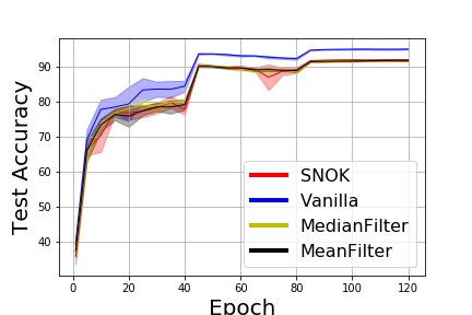
(e) ResNet-Clean

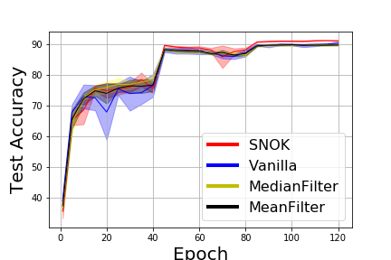
(f) ResNet-Gaussian-0.1

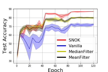
(g) ResNet-Gaussian-0.2

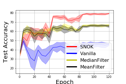
(h) ResNet-Gaussian-0.3

Figure 3: Mean test accuracy $\pm$ std over 5 independent runs on CIFAR10 dataset with Gaussian noise for DenseNet and ResNet backbone

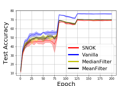
(a) DenseNet-Clean

(b) DenseNet-Gaussian-0.1

(c) DenseNet-Gaussian-0.2

(d) DenseNet-Gaussian-0.3

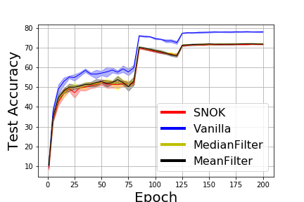
(e) ResNet-Clean

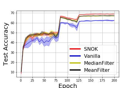
(f) ResNet-Gaussian-0.1

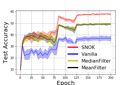
(g) ResNet-Gaussian-0.2

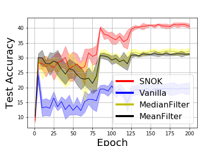
(h) ResNet-Gaussian-0.3

Figure 4: Mean test accuracy $\pm$ std over 5 independent runs on CIFAR100 dataset with Gaussian noise for DenseNet and ResNet backbone

(a) DenseNet-Clean

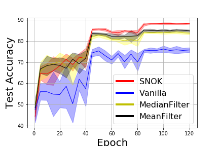
(b) DenseNet-Laplace-0.1

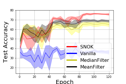
(c) DenseNet-Laplace-0.2

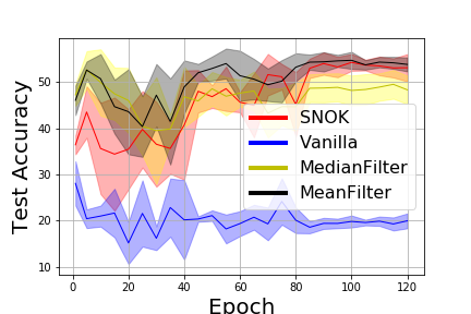
(d) DenseNet-Laplace-0.3

(e) ResNet-Clean

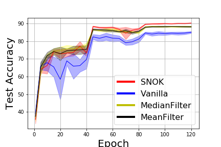
(f) ResNet-Laplace-0.1

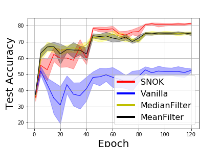
(g) ResNet-Laplace-0.2

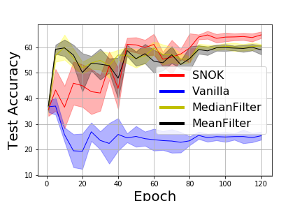
(h) ResNet-Laplace-0.3

Figure 5: Mean test accuracy $\pm$ std over 5 independent runs on CIFAR10 dataset with Laplace noise for DenseNet and ResNet backbone

(a) DenseNet-Clean

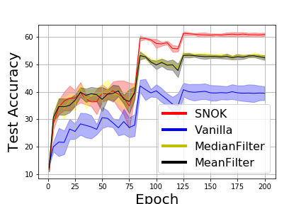
(b) DenseNet-Laplace-0.1

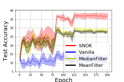
(c) DenseNet-Laplace-0.2

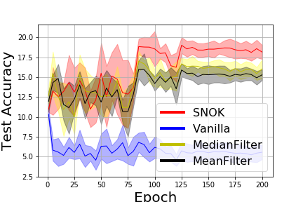
(d) DenseNet-Laplace-0.3

(e) ResNet-Clean

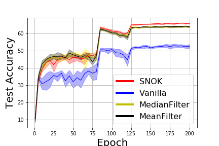
(f) ResNet-Laplace-0.1

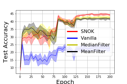
(g) ResNet-Laplace-0.2

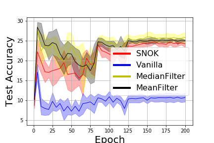
(h) ResNet-Laplace-0.3

Figure 6: Mean test accuracy $\pm$ std over 5 independent runs on CIFAR100 dataset with Laplace noise for DenseNet and ResNet backbone

References

[1]
Zeyuan Allen-Zhu and Yuanzhi Li.
What can resnet learn efficiently, going beyond kernels?
arXiv preprint arXiv:1905.10337, 2019.
[2]
Zeyuan Allen-Zhu and Yuanzhi Li.
Backward feature correction: How deep learning performs deep
learning.
arXiv preprint arXiv:2001.04413, 2020.
[3]
Sanjeev Arora, Simon S Du, Wei Hu, Zhiyuan Li, Ruslan Salakhutdinov, and
Ruosong Wang.
On exact computation with an infinitely wide neural net.
arXiv preprint arXiv:1904.11955, 2019.
[4]
Ainesh Bakshi, Rajesh Jayaram, and David P Woodruff.
Learning two layer rectified neural networks in polynomial time.
In Conference on Learning Theory, pages 195–268. PMLR, 2019.
[5]
Peter L Bartlett and Shahar Mendelson.
Rademacher and gaussian complexities: Risk bounds and structural
results.
Journal of Machine Learning Research, 3(Nov):463–482, 2002.
[6]
Digvijay Boob and Guanghui Lan.
Theoretical properties of the global optimizer of two layer neural
network.
arXiv preprint arXiv:1710.11241, 2017.
[7]
Youngmin Cho and Lawrence K. Saul.
Kernel methods for deep learning.
In NIPS, 2009.
[8]
Amit Daniely, Roy Frostig, and Yoram Singer.
Toward deeper understanding of neural networks: The power of
initialization and a dual view on expressivity.
arXiv preprint arXiv:1602.05897, 2016.
[9]
David L Donoho, Iain M Johnstone, Jeffrey C Hoch, and Alan S Stern.
Maximum entropy and the nearly black object.
Journal of the Royal Statistical Society: Series B
(Methodological), 54(1):41–67, 1992.
[10]
David L Donoho and Jain M Johnstone.
Ideal spatial adaptation by wavelet shrinkage.
biometrika, 81(3):425–455, 1994.
[11]
Simon S Du, Xiyu Zhai, Barnabas Poczos, and Aarti Singh.
Gradient descent provably optimizes over-parameterized neural
networks.
arXiv preprint arXiv:1810.02054, 2018.
[12]
Ronen Eldan and Ohad Shamir.
The power of depth for feedforward neural networks.
In Conference on learning theory, pages 907–940. PMLR, 2016.
[13]
Jianqing Fan and Runze Li.
Variable selection via nonconcave penalized likelihood and its oracle
properties.
Journal of the American statistical Association,
96(456):1348–1360, 2001.
[14]
Behrooz Ghorbani, Song Mei, Theodor Misiakiewicz, and Andrea Montanari.
Linearized two-layers neural networks in high dimension.
The Annals of Statistics, 49(2):1029–1054, 2021.
[15]
Ian Goodfellow, Yoshua Bengio, and Aaron Courville.
Deep learning.
MIT press, 2016.
[16]
Ian J Goodfellow, Jonathon Shlens, and Christian Szegedy.
Explaining and harnessing adversarial examples.
ICLR, 2015.
[17]
Boris Hanin and Mihai Nica.
Finite depth and width corrections to the neural tangent kernel.
arXiv preprint arXiv:1909.05989, 2019.
[18]
Kaiming He, Xinlei Chen, Saining Xie, Yanghao Li, Piotr Dollár, and Ross
Girshick.
Masked autoencoders are scalable vision learners.
arXiv preprint arXiv:2111.06377, 2021.
[19]
Kaiming He, Xiangyu Zhang, Shaoqing Ren, and Jian Sun.
Deep residual learning for image recognition.
In Proceedings of the IEEE conference on computer vision and
pattern recognition, pages 770–778, 2016.
[20]
Kyle Helfrich, Devin Willmott, and Qiang Ye.
Orthogonal recurrent neural networks with scaled cayley transform.
In International Conference on Machine Learning, pages
1969–1978. PMLR, 2018.
[21]
Kurt Hornik, Maxwell Stinchcombe, and Halbert White.
Multilayer feedforward networks are universal approximators.
Neural networks, 2(5):359–366, 1989.
[22]
Gao Huang, Zhuang Liu, Laurens Van Der Maaten, and Kilian Q Weinberger.
Densely connected convolutional networks.
In Proceedings of the IEEE conference on computer vision and
pattern recognition, pages 4700–4708, 2017.
[23]
Arthur Jacot, Franck Gabriel, and Clément Hongler.
Neural tangent kernel: Convergence and generalization in neural
networks.
arXiv preprint arXiv:1806.07572, 2018.
[24]
Kenji Kawaguchi.
Deep learning without poor local minima.
Advances in Neural Information Processing Systems, 2016.
[25]
Alex Krizhevsky, Geoffrey Hinton, et al.
Learning multiple layers of features from tiny images.
2009.
[26]
Jaehoon Lee, Lechao Xiao, Samuel S Schoenholz, Yasaman Bahri, Roman Novak,
Jascha Sohl-Dickstein, and Jeffrey Pennington.
Wide neural networks of any depth evolve as linear models under
gradient descent.
Neural Information Processing Systems, 2019.
[27]
Moshe Leshno, Vladimir Ya Lin, Allan Pinkus, and Shimon Schocken.
Multilayer feedforward networks with a nonpolynomial activation
function can approximate any function.
Neural networks, 6(6):861–867, 1993.
[28]
Yuanzhi Li and Yingyu Liang.
Learning overparameterized neural networks via stochastic gradient
descent on structured data.
arXiv preprint arXiv:1808.01204, 2018.
[29]
Yueming Lyu.
Spherical structured feature maps for kernel approximation.
In International Conference on Machine Learning, pages
2256–2264, 2017.
[30]
Yueming Lyu, Yuan Yuan, and Ivor W Tsang.
Subgroup-based rank-1 lattice quasi-monte carlo.
In NeurIPS, 2020.
[31]
Volodymyr Mnih, Koray Kavukcuoglu, David Silver, Alex Graves, Ioannis
Antonoglou, Daan Wierstra, and Martin Riedmiller.
Playing atari with deep reinforcement learning.
arXiv preprint arXiv:1312.5602, 2013.
[32]
Atsushi Nitanda and Taiji Suzuki.
Optimal rates for averaged stochastic gradient descent under neural
tangent kernel regime.
ICLR, 2021.
[33]
Carl Olsson, Marcus Carlsson, Fredrik Andersson, and Viktor Larsson.
Non-convex rank/sparsity regularization and local minima.
In Proceedings of the IEEE International Conference on Computer
Vision, pages 332–340, 2017.
[34]
Peter H Schönemann.
A generalized solution of the orthogonal procrustes problem.
Psychometrika, 31(1):1–10, 1966.
[35]
Vaishaal Shankar, Alex Fang, Wenshuo Guo, Sara Fridovich-Keil, Jonathan
Ragan-Kelley, Ludwig Schmidt, and Benjamin Recht.
Neural kernels without tangents.
In International Conference on Machine Learning, pages
8614–8623. PMLR, 2020.
[36]
Rupesh Kumar Srivastava, Klaus Greff, and Jürgen Schmidhuber.
Training very deep networks.
NeurIPS, 2015.
[37]
Thomas Wolf, Lysandre Debut, Victor Sanh, Julien Chaumond, Clement Delangue,
Anthony Moi, Pierric Cistac, Tim Rault, Rémi Louf, Morgan Funtowicz,
et al.
Huggingface’s transformers: State-of-the-art natural language
processing.
arXiv preprint arXiv:1910.03771, 2019.
[38]
Cihang Xie, Yuxin Wu, Laurens van der Maaten, Alan L Yuille, and Kaiming He.
Feature denoising for improving adversarial robustness.
In Proceedings of the IEEE/CVF Conference on Computer Vision and
Pattern Recognition, pages 501–509, 2019.
[39]
Gilad Yehudai and Ohad Shamir.
On the power and limitations of random features for understanding
neural networks.
arXiv preprint arXiv:1904.00687, 2019.
[40]
Felix X Yu, Ananda Theertha Suresh, Krzysztof Choromanski, Daniel
Holtmann-Rice, and Sanjiv Kumar.
Orthogonal random features.
arXiv preprint arXiv:1610.09072, 2016.
[42]
Cun-Hui Zhang et al.
Nearly unbiased variable selection under minimax concave penalty.
The Annals of statistics, 38(2):894–942, 2010.
[43]
Tong Zhang.
Analysis of multi-stage convex relaxation for sparse regularization.
Journal of Machine Learning Research, 11(3), 2010.
[44]
Difan Zou and Quanquan Gu.
An improved analysis of training over-parameterized deep neural
networks.
Advances in Neural Information Processing Systems, 2019.