Unbalanced Optimal Transport through Non-negative Penalized Linear Regression

Abstract

This paper addresses the problem of Unbalanced Optimal Transport (UOT) in which the marginal conditions are relaxed (using weighted penalties in lieu of equality) and no additional regularization is enforced on the OT plan. In this context, we show that the corresponding optimization problem can be reformulated as a non-negative penalized linear regression problem. This reformulation allows us to propose novel algorithms inspired from inverse problems and nonnegative matrix factorization. In particular, we consider majorization-minimization which leads in our setting to efficient multiplicative updates for a variety of penalties. Furthermore, we derive for the first time an efficient algorithm to compute the regularization path of UOT with quadratic penalties. The proposed algorithm provides a continuity of piece-wise linear OT plans converging to the solution of balanced OT (corresponding to infinite penalty weights). We perform several numerical experiments on simulated and real data illustrating the new algorithms, and provide a detailed discussion about more sophisticated optimization tools that can further be used to solve OT problems thanks to our reformulation.

1 Introduction

Optimal Transport (OT) theory provides powerful tools for comparing probability distributions and has been successfully employed in a wide range of machine learning applications such as supervised learning (Frogner et al., 2015), clustering (Ho et al., 2017), generative modelling (Arjovsky et al., 2017), domain adaptation (Courty et al., 2017), learning of structured data (Maretic et al., 2019; Vayer et al., 2019) or natural language processing (Kusner et al., 2015), among many others. One reason for those recent successes is the introduction of entropy-regularized OT that can be solved with the efficient Sinkhorn-Knopp matrix scaling algorithm (Cuturi, 2013). However, the classical OT problem seeks the optimal cost to transport all the mass from a source distribution to a target one (Villani, 2009), greatly limiting its use in scenarii where the measures have different masses or when they contain noisy observations or outliers.

Unbalanced Optimal Transport (UOT) (Benamou, 2003) has been introduced to tackle this shortcoming, allowing some mass variation in the transportation problem. It is expressed as a relaxation of the Kantorovich formulation (Kantorovich, 1942) by penalizing the divergence between the marginals of the transportation plan and the given distributions. Several divergences can be considered, such as the Kullback-Leiber (KL) divergence (Frogner et al., 2015; Liero et al., 2018), the $\ell_{1}$ norm corresponding to the partial optimal transport problem (Caffarelli and McCann, 2010; Figalli, 2010), or the squared $\ell_{2}$ norm (Benamou, 2003). Regarding numerical solutions, Chizat et al. (2018) considered an entropic-regularized version of UOT leading to a class of scaling algorithms in the vein of the Sinkhorn-Knopp approach (Sinkhorn and Knopp, 1967). The introduction of this entropic regularization improves the scalability of OT, but involves a spreading of the mass and a loss of sparsity in the OT plan. When a sparse transport plan is sought, the convergence is slowed down, necessitating the use of acceleration strategies (Thibault et al., 2021). Regarding UOT with the (squared) $\ell_{2}$ norm, Blondel et al. (2018) showed that the resulting OT plan is sparse and proposed to use an efficient L-BFGS-B algorithm (Byrd et al., 1995) to address this case. Note that the L-BFGS-B method can be used to solve UOT with differentiable divergences even without the entropic-regularization on the OT plan that induces the Sinkhorn-like iterations. Finally, also note that, as for balanced OT, UOT can be solved more efficiently when the data has a specific structure, such as unidimensional distributions (Bonneel and Coeurjolly, 2019) or distributions supported on trees (Sato et al., 2020).

Contributions.

In this paper, we show after some preliminaries that UOT can be recast as a convex penalized linear regression problem with non-negativity constraints (Section 2.2). The main interest of this reformulation resides in the fact that non-negative linear regression has been extensively studied in inverse problems and machine learning, offering a large panel of tools for devising new numerical algorithms. Our reformulation involves a design/dictionary matrix that is structured and sparse. Leveraging this structure, we propose two new families of algorithms for solving the exact (i.e., without regularization of the plan) UOT problem in Section 3.

We first derive in Section 3.1 a new Majorization-Minimization (MM) algorithm for solving UOT with Bregman divergences, and more specifically KL and $\ell_{2}$-penalized UOT. The MM approach results in multiplicative updates that have appealing features: i) they are easy to implement, ii) have low complexity per iteration and can be instantiated on GPU, iii) ensure monotonicity of the objective function and inherit existing convergence results. Our methodology is inspired by well-known algorithms in image restoration (Richardson, 1972; De Pierro, 1993) and non-negative matrix factorization (NMF) (Lee and Seung, 2001; Dhillon and Sra, 2005; Févotte and Idier, 2011). Interestingly, the resulting multiplicative updates bear a similarity with the celebrated Sinkhorn scaling algorithm, with some key differences that are discussed.

Next, we derive in Section 3.2 an efficient algorithm to compute the regularization path in $\ell_{2}$-penalized UOT. To do so, we build on our proposed reformulation and more precisely on the fact that $\ell_{2}$-penalized UOT can be reformulated as a weighted Lasso problem. We propose a new methodology inspired by LARS (Efron et al., 2004; Hastie et al., 2004), which, to the best of our knowledge, is the first regularization path algorithm for OT problems. It brings a novel understanding of the properties of the evolution of the support of OT plans, besides the practical interest of computing the complete regularization path when hyperparameter validation is necessary.

Our new families of algorithms (MM for general UOT, LARS for $\ell_{2}$-penalized UOT) are showcased in the numerical experiments of Section 4. Python implementation of the algorithms, provided in supplementary, will be released with MIT license on GitHub. The connection between UOT and linear regression that we reveal in the paper opens the door to further fruitful developments and in particular to more efficient algorithms, thanks to the large literature dealing with non-negative penalized linear regression. We discuss those possible research directions in Section 5, before concluding the paper.

Notations.

Vectors such as $\boldsymbol{m}$ are written with lower case and bold font, with coefficients $m_{i}$ or $[\boldsymbol{m}]_{i}$, according to context. The $|\mathcal{A}|$-dimensional sub-vector with indexes in set $\mathcal{A}$ is written $\boldsymbol{m}_{\mathcal{A}}$. Matrices such as $\boldsymbol{M}$ are written with upper case and bold font, with coefficients $M_{i,j}$. We introduce a vectorization operator defined by $\boldsymbol{m}=\text{vec}(\boldsymbol{M})=[M_{1,1},M_{1,2},\dots,M_{n,m-1},M_{n,m}]^{\top}$, i.e., the concatenation of the rows of the matrix, following the Numpy/C memory convention. $\mathds{1}_{n}$ is a vector of $n$ ones and $\boldsymbol{M}\geq 0$ denotes entry-wise non-negativity. Finally, $D_{\varphi}$ is the Bregman divergence generated by the strictly convex and differentiable function $\varphi$, i.e., $D_{\varphi}(\boldsymbol{u},\boldsymbol{v})=\sum_{i}d_{\varphi}(u_{i},v_{i})=\sum_{i}[\varphi(u_{i})-\varphi(v_{i})-\varphi^{\prime}(v_{i})(u_{i}-v_{i})]$.

2 Reformulation of UOT as non-negative penalized linear regression

2.1 Background on Optimal Transport

Let us consider two clouds of points $\boldsymbol{X}=\{\boldsymbol{x}_{i}\}^{n}_{i=1}$ and $\boldsymbol{Y}=\{\boldsymbol{y}_{j}\}^{m}_{j=1}$. Let $\boldsymbol{a}\in\mathbb{R}^{+}_{n}$ and $\boldsymbol{b}\in\mathbb{R}^{+}_{m}$ be two discrete distributions of mass on $\boldsymbol{X}$ and $\boldsymbol{Y}$, such that $a_{i}$ (resp. $b_{j}$) is the mass at $\boldsymbol{x}_{i}$ (resp. $\boldsymbol{y}_{j}$). The balanced OT problem, as defined by Kantorovich (1942), is a linear problem that computes the minimum cost of moving $\boldsymbol{a}$ to $\boldsymbol{b}$:

$$\text{OT}(\boldsymbol{a},\boldsymbol{b})=\min_{\boldsymbol{T}\geq 0}\langle\boldsymbol{C},\boldsymbol{T}\rangle\quad\text{such that (s.t.)}\quad\boldsymbol{T}\mathds{1}_{m}=\boldsymbol{a},\boldsymbol{T}^{\top}\mathds{1}_{n}=\boldsymbol{b}$$ (1)

where $\langle\cdot,\cdot\rangle$ is the Frobenius inner product, $\boldsymbol{T}\in\mathbb{R}^{+}_{n\times m}$ is the transport plan and $\boldsymbol{C}\in\mathbb{R}^{+}_{n\times m}$ is the cost matrix. The entry $C_{i,j}$ of $\boldsymbol{C}$ represents the cost of moving point $\boldsymbol{x}_{i}$ to $\boldsymbol{y}_{j}$. The Wasserstein 1-distance (also known as the earth mover’s distance) is obtained for $C_{i,j}=\|\boldsymbol{x}_{i}-\boldsymbol{y}_{j}\|$. The constraints on the transport plan $\boldsymbol{T}$ require that $\|\boldsymbol{a}\|_{1}=\|\boldsymbol{b}\|_{1}$ and that all the mass from $\boldsymbol{a}$ is transported to $\boldsymbol{b}$. These constraints can be alleviated through relaxation, leading to UOT (Benamou, 2003):

$$\text{UOT}^{\boldsymbol{\lambda}}(\boldsymbol{a},\boldsymbol{b})=\min_{\boldsymbol{T}\geq 0}\quad\langle\boldsymbol{C},\boldsymbol{T}\rangle+\lambda_{1}D_{\varphi}(\boldsymbol{T}\mathds{1}_{m},\boldsymbol{a})+\lambda_{2}D_{\varphi}(\boldsymbol{T}^{\top}\mathds{1}_{n},\boldsymbol{b}).$$ (2)

The deviations from the true marginals are penalized by means of a given Bregman divergence $D_{\varphi}$, as introduced in Chizat et al. (2018), where $\lambda_{1}$ and $\lambda_{2}$ are hyperparameters that represent the strengths of penalization. Note that balanced OT (1) is recovered when $\lambda_{1}=\lambda_{2}\to\infty$. Furthermore, when $\lambda_{1}$ or $\lambda_{2}\to\infty$, we recover semi-relaxed OT (Rabin et al., 2014). In practice, authors often set $\lambda_{1}=\lambda_{2}=\lambda$ for UOT in order to reduce the necessity of hyperparameter tuning. Various divergences have been considered in the literature. The $\ell_{1}$ norm gives rise to so-called partial optimal transport (Caffarelli and McCann, 2010). The squared $\ell_{2}$ norm provides a sparse and smooth transport plan (Blondel et al., 2018) when introducing a strongly convex term in Eq. (2). Chizat et al. (2018) derive efficient algorithms to solve Eq. (2) for several divergences by adding an additional regularization term $\lambda_{\text{reg}}D_{\varphi}(\boldsymbol{T},\boldsymbol{a}\boldsymbol{b}^{\top})$. In particular, entropic regularization is obtained when the KL divergence is used, promoting a dense transport plan unlike exact UOT.

2.2 Reformulation of UOT

UOT cast as regression.

Let $\boldsymbol{t}=\text{vec}(\boldsymbol{T})$, $\boldsymbol{c}=\text{vec}(\boldsymbol{C})$ and $\boldsymbol{y}^{\top}=[\boldsymbol{a}^{\top},\boldsymbol{b}^{\top}]$. Problem (2) can be re-written as

$$\min_{\boldsymbol{t}\geq 0}\quad F_{\lambda}(\boldsymbol{t})\stackrel{{\scriptstyle\text{def}}}{{=}}\frac{1}{\lambda}\boldsymbol{c}^{\top}\boldsymbol{t}+D_{\varphi}(\boldsymbol{H}\boldsymbol{t},\boldsymbol{y})$$ (3)

and as such be expressed as a non-negative penalized linear regression problem, where the design matrix $\boldsymbol{H}=[\boldsymbol{H}_{r}^{\top},\boldsymbol{H}_{c}^{\top}]^{\top}$ is the concatenation of the matrices $\boldsymbol{H}_{r}$ and $\boldsymbol{H}_{c}$ that compute sums of the rows and columns of $\boldsymbol{T}$, respectively (see expressions in Section A.1 of the supplementary material). Note that, for the sake of simplicity, we consider here $\lambda_{1}=\lambda_{2}=\lambda$ but this hypothesis could be easily alleviated for a given family of divergences (see Sec. 5 for a discussion). Important features of Eq. (3) should be discussed. First, $F_{\lambda}(\boldsymbol{t})$ is convex thanks to the convexity of Bregman divergences w.r.t. their first argument. Second, $\boldsymbol{H}$ is very structured and sparse (with a ratio of only $\frac{1}{m+n}$ non-zero coefficients) which will allow for more efficient computations and updates than with a dense $\boldsymbol{H}$. Finally, since $\boldsymbol{t}\geq 0$ and $\boldsymbol{c}\geq 0$, the linear term can be expressed as $\frac{1}{\lambda}\boldsymbol{c}^{\top}\boldsymbol{t}=\frac{1}{\lambda}\sum_{i}c_{i}t_{i}=\frac{1}{\lambda}\sum_{i}c_{i}|t_{i}|$. This corresponds to a weighted $\ell_{1}$ regularization, promoting sparsity in $\boldsymbol{t}$ and hence in the transport plans. Note that the “sparse” regularization is here controlled by $\frac{1}{\lambda}$ (instead of $\lambda$ in classical penalized linear regression), meaning that the sparsity promoting term will be more aggressive for small $\lambda$.

Solving problem (3).

Problems of the form of Eq. (3) are well-known in inverse problems and NMF. In inverse problems, $\boldsymbol{t}$ typically acts as a clean image degraded by operator $\boldsymbol{H}$ (e.g., a convolution) and noise. The data fitting term $D_{\varphi}(\boldsymbol{H}\boldsymbol{t},\boldsymbol{y})$ captures assumptions about the noise corrupting the observed image $\boldsymbol{y}$. Sparsity is a common regularizer of $\boldsymbol{t}$. In NMF, given a set of nonnegative samples $\{\boldsymbol{y}_{l}\}$ one wants to learn a non-negative dictionary $\boldsymbol{H}$ and non-negative lower-dimensional embeddings $\{\boldsymbol{t}_{l}\}$ such that $\boldsymbol{y}_{l}\approx\boldsymbol{H}\boldsymbol{t}_{l}$ (Lee and Seung, 1999). Updating the latter involves optimization problems of form (3) (with or without sparse regularization). In contrast to problem (3), the data fitting term is more commonly $D_{\varphi}(\boldsymbol{y},\boldsymbol{H}\boldsymbol{t})$ instead of $D_{\varphi}(\boldsymbol{H}\boldsymbol{t},\boldsymbol{y})$ in inverse problems and NMF. This is because the former is a log-likelihood in disguise for the mean-parametrized exponential family, and takes important noise models as special cases, such as Poisson, additive Gaussian or multiplicative Gamma noise (Févotte and Idier, 2011). Using such penalizations with reversed arguments would be possible in our case as well but we stick to the now standard formulation of (Liero et al., 2018; Chizat et al., 2018) for simplicity.

In the next section, we will first leverage a classical family of algorithms in inverse problems and NMF, namely MM, to obtain new algorithms for KL and $\ell_{2}$-penalized UOT (possibly with entropic regularization in the first case). Second, we will leverage results about non-negative Lasso to design an efficient algorithm to compute the regularization path of $\ell_{2}$-penalized UOT.

3 Novel numerical solvers for UOT

3.1 Majorization-Minimization (MM) for UOT

General MM framework.

MM algorithms have been around a long time in inverse problems and NMF to solve problems of form (3). Classical algorithms for NMF such as (Lee and Seung, 2001) have built on seminal MM algorithms for inverse problems such as (Richardson, 1972; De Pierro, 1993). Subsequent works in NMF such as (Dhillon and Sra, 2005; Févotte and Idier, 2011; Yang and Oja, 2011) have further contributed novel MM algorithms for larger classes of problems, including larger families of divergences. In a nutshell, MM consists in iteratively building and minimizing an upper bound of the objective function which is tight at the current parameter estimate (and referred to as auxiliary function), see Hunter and Lange (2004); Sun et al. (2017) for tutorials. In NMF, a common approach consists of alternating the updates of the dictionary $\boldsymbol{H}$ and of the embeddings. In our case, $\boldsymbol{H}$ is fixed and we may use the results of (Dhillon and Sra, 2005) to build an auxiliary function for term $D_{\varphi}(\boldsymbol{H}\boldsymbol{t},\boldsymbol{y})$, to which we may simply add the linear term $\boldsymbol{c}^{\top}\boldsymbol{t}/\lambda$ to obtain a valid auxiliary function for $F_{\lambda}(\boldsymbol{t})$. Let $\tilde{\boldsymbol{t}}$ denote the current estimate of $\boldsymbol{t}$, $\tilde{Z}_{i,j}=\frac{H_{i,j}\tilde{t}_{j}}{\sum_{l}H_{i,l}\tilde{t}_{l}}$ and

$$G_{\lambda}(\boldsymbol{t},\tilde{\boldsymbol{t}})=\sum_{i,j}\tilde{Z}_{i,j}\varphi\left(\frac{H_{i,j}t_{j}}{\tilde{Z}_{i,j}}\right)+\sum_{j}\left[\frac{c_{j}}{\lambda}-\sum_{i}H_{i,j}\varphi^{\prime}(y_{i})\right]t_{j}+cst,$$ (4)

where $cst=\sum_{i}[\varphi^{\prime}(y_{i})y_{i}-\varphi(y_{i}]$. Then, $G_{\lambda}(\boldsymbol{t},\tilde{\boldsymbol{t}})$ is an auxiliary function for $F_{\lambda}(\boldsymbol{t})$, i.e., $\forall\boldsymbol{t}$, $G_{\lambda}(\boldsymbol{t},\tilde{\boldsymbol{t}})\geq F_{\lambda}(\boldsymbol{t})$ and $G_{\lambda}(\tilde{\boldsymbol{t}},\tilde{\boldsymbol{t}})=F_{\lambda}(\tilde{\boldsymbol{t}})$. Let $\boldsymbol{t}^{(k+1)}=\text{argmin}_{\boldsymbol{t}\geq 0}G_{\lambda}({\boldsymbol{t}},\boldsymbol{t}^{(k)})$, then $F_{\lambda}(\boldsymbol{t}^{(k)})=G_{\lambda}(\boldsymbol{t}^{(k)},\boldsymbol{t}^{(k)})\geq G_{\lambda}(\boldsymbol{t}^{(k+1)},\boldsymbol{t}^{(k)})\geq F_{\lambda}(\boldsymbol{t}^{(k+1)})$, producing a descent algorithm over $F$. The trick to obtain $G$ is to apply Jensen inequality to $\varphi(\sum_{j}H_{i,j}t_{j})=\varphi(\sum_{j}\tilde{Z}_{i,j}\frac{H_{i,j}}{\tilde{Z}_{i,j}}t_{j})\leq\sum_{j}\tilde{Z}_{i,j}\varphi(\frac{H_{i,j}}{\tilde{Z}_{i,j}}t_{j})$, thanks to the convexity of $\varphi$, see details in (Dhillon and Sra, 2005). We provide below the resulting algorithms for the KL and $\ell_{2}$ penalizations, with detailed computations available in Section A.2 of the supplementary.

MM for KL-penalized UOT.

The KL divergence is obtained with $\varphi(y)=y\log y-y$. Minimizing $G_{\lambda}(\boldsymbol{t},\boldsymbol{t}^{(k)})$ in that case leads to following multiplicative update:

$$t_{j}^{(k+1)}=t^{(k)}_{j}\,\exp\left(\frac{[\boldsymbol{H}^{\top}\log(\boldsymbol{y})-\boldsymbol{H}^{\top}\log\left(\boldsymbol{H}\boldsymbol{t}^{(k)}\right)]_{j}-\frac{1}{\lambda}c_{j}}{[\boldsymbol{H}^{\top}\mathds{1}]_{j}}\right).$$ (5)

Owing to the structure of $\boldsymbol{t}$ and $\boldsymbol{H}$, the update can be re-written in the following matrix form:

$$\boldsymbol{T}^{(k+1)}=\text{diag}\left(\frac{\boldsymbol{a}}{\boldsymbol{T}^{(k)}\mathds{1}_{m}}\right)^{\frac{1}{2}}\left(\boldsymbol{T}^{(k)}\odot\text{exp}\left(-\frac{\boldsymbol{C}}{2\lambda}\right)\right)\text{diag}\left(\frac{\boldsymbol{b}}{{\boldsymbol{T}^{(k)\top}}\mathds{1}_{n}}\right)^{\frac{1}{2}},$$ (6)

where $\odot$ is entrywise multiplication and divisions are taken entrywise as well. The multiplicative update (6) is remarkably similar to the well-known Sinkhorn-Knopp algorithm that has been used in numerous OT problems involving KL regularization. But instead of two separate steps for the left and right scaling, Eq. (6) applies these scalings simultaneously in a unique update using the diagonal matrices (and a form of geometrical average). Also note how the scaling factor $\text{exp}\left(-\frac{\boldsymbol{C}}{2\lambda}\right)$ penalizes along iterations the coefficients of the transport plan with large costs.

MM for $\ell_{2}$-penalized UOT.

The quadratic loss is obtained with $\varphi(y)=\frac{y^{2}}{2}$. In that case, minimizing $G_{\lambda}(\boldsymbol{t},\boldsymbol{t}^{(k)})$ s.t. non-negativity leads to following multiplicative update:

$$\boldsymbol{T}^{(k+1)}=\boldsymbol{T}^{(k)}\odot\frac{\max\left(0,\boldsymbol{a}\mathds{1}_{m}^{\top}+\mathds{1}_{n}\boldsymbol{b}^{\top}-\frac{1}{\lambda}\boldsymbol{C}\right)}{\boldsymbol{T}^{(k)}\mathbf{O}_{m}+\mathbf{O}_{n}\boldsymbol{T}^{(k)}}\quad\text{with}\quad\mathbf{O}_{\ell}=\mathds{1}_{\ell}\mathds{1}_{\ell}^{\top}.$$ (7)

Interestingly enough, update (7) prunes any coefficient $T_{i,j}$ in $\boldsymbol{T}$ such that $a_{i}+b_{j}-\frac{1}{\lambda}C_{i,j}<0$ from the very first iteration, providing a useful certificate on the support of the solution.

3.2 Regularization path for $\ell_{2}$-penalized UOT

Let us focus on the case where $D_{\varphi}$ is a quadratic divergence. As mentioned in Section 2.2, Eq. (3) is then a positive weighted Lasso problem, allowing us to derive the first regularization path algorithm for computing the whole set of solutions for a varying $\lambda$ from 0 to $+\infty$. Note that the path’s extreme point recovers the balanced OT solution. We show that the path is piecewise linear in $1/\lambda$ between changes in the active set $\mathcal{A}=\text{supp}(\boldsymbol{t}^{\lambda})$, where $\boldsymbol{t}^{\lambda}=\text{vec}(\boldsymbol{T}^{\lambda})$ and $\boldsymbol{T}^{\lambda}$ is the OT plan for given hyperparameter $\lambda$. The main steps of the algorithm are roughly as follows: given a current solution $(\lambda_{k},\boldsymbol{T}^{\lambda_{k}})$ and a current active set $\mathcal{A}_{k}$, we look for the next value $\lambda_{k+1}>\lambda_{k}$ such that the active set changes (i.e., $\mathcal{A}_{k+1}\neq\mathcal{A}_{k}$), either because one component enters or leaves the active set. We describe our algorithm below.

KKT conditions of the $\ell_{2}$-penalized UOT problem.

The Lagrangian for problem (3) writes:

$${L}_{\lambda}(\boldsymbol{t},\boldsymbol{\gamma})=\frac{1}{\lambda}\boldsymbol{c}^{\top}\boldsymbol{t}+{\frac{1}{2}}(\boldsymbol{H}\boldsymbol{t}-\boldsymbol{y})^{\top}(\boldsymbol{H}\boldsymbol{t}-\boldsymbol{y})-\boldsymbol{\gamma}^{\top}\boldsymbol{t}$$ (8)

where $\boldsymbol{\gamma}$ represents the Lagrange parameters. We denote $\boldsymbol{m}=\boldsymbol{H}^{\top}\boldsymbol{y}=\text{vec}(\boldsymbol{a}{\mathds{1}_{m}^{\top}}+{\mathds{1}_{n}}\boldsymbol{b}^{\top})$. KKT optimality conditions state that i) $\nabla_{\boldsymbol{t}}{L}_{\lambda}(\boldsymbol{t},\lambda)=\frac{1}{\lambda}\boldsymbol{c}+\boldsymbol{H}^{\top}\boldsymbol{H}\boldsymbol{t}-\boldsymbol{m}-\boldsymbol{\gamma}=0$ (stationarity condition), ii) $\boldsymbol{\gamma}\odot\boldsymbol{t}=0$ (complementary condition) and iii) $\boldsymbol{\gamma}\geq 0$ (feasibility condition).

Piecewise linearity of the path.

Assume that, at iteration $k$, we know the current active set $\mathcal{A}=\mathcal{A}_{k}$ and we look for $\boldsymbol{t}_{\mathcal{A}}^{\lambda}$ (the other values of $\boldsymbol{t}_{\mathcal{A}}$ being $0$). Let $\boldsymbol{H}_{\mathcal{A}}$, $\boldsymbol{m}_{A}$ and $\boldsymbol{c}_{\mathcal{A}}$ denote the corresponding sub-matrix and vectors (see Appendix A.3 for rigorous definitions). Because of the complementary condition, we have $\boldsymbol{\gamma}_{\mathcal{A}}=\boldsymbol{0}$. Using $\lambda=\lambda_{k}+\epsilon$, with $\epsilon>0$ small enough to ensure that the active set remains the same, the stationarity condition writes:

$$\boldsymbol{H}_{\mathcal{A}}^{\top}\boldsymbol{H}_{\mathcal{A}}\boldsymbol{t}^{\lambda}_{\mathcal{A}}=\boldsymbol{m}_{\mathcal{A}}-\frac{1}{\lambda}\boldsymbol{c}_{\mathcal{A}} \Rightarrow \boldsymbol{t}_{\mathcal{A}}^{\lambda}=\tilde{\boldsymbol{m}}_{\mathcal{A}}-\frac{1}{\lambda}\tilde{\boldsymbol{c}}_{\mathcal{A}}$$ (9)

with $\tilde{\boldsymbol{m}}_{\mathcal{A}}=(\boldsymbol{H}_{\mathcal{A}}^{\top}\boldsymbol{H}_{\mathcal{A}})^{-1}{\boldsymbol{m}}_{\mathcal{A}}$ and $\tilde{\boldsymbol{c}}_{\mathcal{A}}=(\boldsymbol{H}_{\mathcal{A}}^{\top}\boldsymbol{H}_{\mathcal{A}})^{-1}{\boldsymbol{c}}_{\mathcal{A}}$ . Eq. (9) shows that the optimal $\boldsymbol{t}_{\mathcal{A}}^{\lambda}$ (and hence $\boldsymbol{t}^{\lambda}$) can be solved for any $\lambda\in[\lambda_{k},\lambda_{k+1}]$, i.e., when the active set $\mathcal{A}$ remains the same, by solving a linear problem. It also reveals the piecewise linearity in $\lambda^{-1}$ of the path when $\mathcal{A}$ is fixed. As expected, balanced OT is recovered when $\lambda\to\infty$.

Finding $(\lambda_{k+1},\mathcal{A}_{k+1})$ given $(\lambda_{k},\mathcal{A}_{k})$.

Given a current solution $(\lambda_{k},\boldsymbol{t}^{\lambda_{k}})$ and $\lambda=\lambda_{k}+\epsilon$, we increase the $\epsilon$ until we reach a change in the set of active components. This happens whenever the first of the following two situations occurs.

$\bullet$ One component in $\mathcal{A}$ becomes inactive. In that case, we remove the index $i\in\mathcal{A}$ with the smallest $\lambda_{r}>\lambda_{k}$ that violates the constraint. In such case, $[\tilde{\boldsymbol{m}}_{\mathcal{A}}]_{i}=[\tilde{\boldsymbol{c}}_{\mathcal{A}}]_{i}/\lambda$ and we may write

$$\lambda_{r}=\min_{>\lambda_{k}}\left(\frac{\tilde{\boldsymbol{c}}_{\mathcal{A}}}{\tilde{\boldsymbol{m}}_{\mathcal{A}}}\right)$$ (10)

where $\min_{>\lambda_{k}}$ indicates the minimum value in the vector greater than $\lambda_{k}$ and the division is entrywise.

$\bullet$ One component in $\bar{\mathcal{A}}$ becomes active. This occurs when the KKT positivity constraint $\boldsymbol{\gamma}_{\bar{\mathcal{A}}}\geq\mathbf{0}$ becomes violated. Assume this happens at index $i\in\bar{\mathcal{A}}$ for the smallest value $\lambda_{a}>\lambda_{k}$ of $\lambda$. In such case, the stationarity condition outside the active set can be rewritten:

$$\left[\frac{1}{\lambda}\boldsymbol{c}_{\bar{\mathcal{A}}}+\Big{[}\boldsymbol{H}^{\top}\boldsymbol{H}\big{(}\tilde{\boldsymbol{m}}+\frac{1}{\lambda}\tilde{\boldsymbol{c}}\big{)}\Big{]}_{\bar{\mathcal{A}}}-\boldsymbol{m}_{\bar{\mathcal{A}}}\right]_{i}=[\boldsymbol{\gamma}_{\bar{\mathcal{A}}}]_{i}\ \Rightarrow\ \lambda_{a}=\min_{>\lambda_{k}}\left(\dfrac{\boldsymbol{c}_{\bar{\mathcal{A}}}-\big{[}\boldsymbol{H}^{\top}\boldsymbol{H}\tilde{\boldsymbol{c}}\big{]}_{\bar{\mathcal{A}}}}{\boldsymbol{m}_{\bar{\mathcal{A}}}-\big{[}\boldsymbol{H}^{\top}\boldsymbol{H}\tilde{\boldsymbol{m}}\big{]}_{\bar{\mathcal{A}}}}\right),$$ (11)

where $\tilde{\boldsymbol{m}}$ (resp. $\tilde{\boldsymbol{c}}$) equals $\tilde{\boldsymbol{m}}_{\mathcal{A}}$ (resp. $\tilde{\boldsymbol{c}}_{\mathcal{A}}$) on $\mathcal{A}$ and zero on $\bar{\mathcal{A}}$.

In practice, at each step of the path, we compute both $\lambda_{r}$ and $\lambda_{a}$, set $\lambda_{k+1}=\min\{\lambda_{r},\lambda_{a}\}$ and update the active set accordingly.

Numerical computation of the entire path.

Eq. (9) involves the computation of the matrix $(\boldsymbol{H}_{\mathcal{A}}^{\top}\boldsymbol{H}_{\mathcal{A}})^{-1}$, which is of size $|\mathcal{A}|\times|\mathcal{A}|$. As only one index leaves or enters the active set at each iteration, we can use the Schur complement of the matrix to compute its value from $(\boldsymbol{H}_{\mathcal{A}_{k}}^{\top}\boldsymbol{H}_{\mathcal{A}_{k}})^{-1}$, alleviating the computational burden of the algorithm as it only involves matrix-vector computations (see Section A.3 of supplementary). Algorithm 1 sums up the different steps of the full path computation. At each iteration, we compute $\lambda_{a}$, $\lambda_{r}$, update the inverse matrix $(\boldsymbol{H}_{\mathcal{A}_{k}}^{\top}\boldsymbol{H}_{\mathcal{A}_{k}})^{-1}$ and estimate the solution $\boldsymbol{t}^{\lambda_{k+1}}$ with a complexity of $O(nm)$.

Algorithm 1 Regularization path of $\ell_{2}$-penalized UOT

  Require: $\boldsymbol{a}$, $\boldsymbol{b}$, $\boldsymbol{C}$, $\lambda_{0}=0$, $\boldsymbol{t}_{0}=\boldsymbol{0}$, $\mathcal{A}=\mathcal{A}_{0}=\emptyset$, $k=1$

  $\lambda_{1}=\min\dfrac{\boldsymbol{c}_{\bar{\mathcal{A}}}}{\boldsymbol{m}_{\bar{\mathcal{A}}}}$, $\mathcal{A}=\mathcal{A}_{1}=\arg\min\dfrac{\boldsymbol{c}_{\bar{\mathcal{A}}}}{\boldsymbol{m}_{\bar{\mathcal{A}}}}$, $\boldsymbol{H}_{\mathcal{A}}^{\top}\boldsymbol{H}_{\mathcal{A}}=2$

  $\boldsymbol{t}^{\lambda_{1}}_{\mathcal{A}_{1}}=\frac{\boldsymbol{m}_{{\mathcal{A}}}}{2}-\frac{1}{\lambda_{1}}\frac{\boldsymbol{c}_{\mathcal{A}}}{2}$

  while $(\boldsymbol{H}\boldsymbol{t}^{\lambda_{k}}-\boldsymbol{y})^{\top}(\boldsymbol{H}\boldsymbol{t}^{\lambda_{k}}-\boldsymbol{y})\neq 0$ do

     $\lambda_{r}$, $\lambda_{a}$ $\leftarrow$ Compute as in Eq. (10) and Eq. (11)

     $\lambda_{k+1}\leftarrow\min(\lambda_{r},\lambda_{a})$

     $\boldsymbol{t}^{\lambda_{k+1}}_{\mathcal{A}}\leftarrow(\boldsymbol{H}_{\mathcal{A}}^{\top}\boldsymbol{H}_{\mathcal{A}})^{-1}\boldsymbol{m}_{\mathcal{A}}-\frac{1}{\lambda_{k+1}}(\boldsymbol{H}_{\mathcal{A}}^{\top}\boldsymbol{H}_{\mathcal{A}})^{-1}\boldsymbol{c}_{\mathcal{A}}$

     $\mathcal{A}=\mathcal{A}_{k+1}\leftarrow$ Update active set for next iteration.

     $(\boldsymbol{H}_{\mathcal{A}}^{\top}\boldsymbol{H}_{\mathcal{A}})^{-1}\leftarrow$ Update from $(\boldsymbol{H}_{\mathcal{A}_{k}}^{\top}\boldsymbol{H}_{\mathcal{A}_{k}})^{-1}$ with Schur complement (see supplementary A.3)

     $k\leftarrow k+1$

  end while

  return  $(\lambda_{k},\boldsymbol{t}^{\lambda_{k}})_{k}$

Regularization path of the semi-relaxed $\ell_{2}$-penalized UOT.

As a side result, let us consider the semi-relaxed OT problem $\text{SROT}^{{\lambda}}(\boldsymbol{a},\boldsymbol{b})=\min_{\boldsymbol{T}\geq 0,\boldsymbol{T}^{\top}\mathds{1}_{n}\ =\boldsymbol{b}}\,\,\langle\boldsymbol{C},\boldsymbol{T}\rangle+\lambda\|\boldsymbol{T}\mathds{1}_{m}-\boldsymbol{a}\|^{2}$. The main difference with UOT is that the equality constraint $\boldsymbol{T}^{\top}\mathds{1}_{n}\ =\boldsymbol{b}$ (equivalent to $\boldsymbol{H}_{c}\boldsymbol{t}=\boldsymbol{b}$) must always be met. This leads to the following Lagrangian:

$$L_{\lambda}(\boldsymbol{t},\boldsymbol{\gamma},\boldsymbol{u})=\frac{1}{\lambda}\boldsymbol{c}^{\top}\boldsymbol{t}+{\frac{1}{2}}(\boldsymbol{H}_{r}\boldsymbol{t}-\boldsymbol{a})^{\top}(\boldsymbol{H}_{r}\boldsymbol{t}-\boldsymbol{a})+(\boldsymbol{H}_{c}\boldsymbol{t}-\boldsymbol{b})^{\top}\boldsymbol{u}-\boldsymbol{\gamma}^{\top}\boldsymbol{t},$$ (12)

where $\boldsymbol{u}\in\mathbb{R}^{m}$ contains the Lagrange parameters associated to the $m$ equality constraints. The KKT optimality conditions now dictate that i) $\nabla_{\boldsymbol{t}}{L}_{\lambda}(\boldsymbol{t},\boldsymbol{\gamma},\boldsymbol{u})=\frac{1}{\lambda}\boldsymbol{c}+\boldsymbol{H}_{r}^{\top}\boldsymbol{H}_{r}\boldsymbol{t}-\boldsymbol{H}_{r}^{\top}\boldsymbol{a}+\boldsymbol{H}_{c}^{\top}\boldsymbol{u}-\boldsymbol{\gamma}=0$, ii) $\boldsymbol{\gamma}\odot\boldsymbol{t}=0$, iii) $\boldsymbol{\gamma}\geq 0$ and $\boldsymbol{H}_{c}\boldsymbol{t}-\boldsymbol{b}=\boldsymbol{0}$. We can use the same reasoning than previously to compute the entire path. Details are provided in Section A.4 of the supplementary. The main difference lies in solving, at each iteration, a linear system of size $(m+|\mathcal{A}|)$ to comply with the marginal equality constraint. The path is initialized as follows: the $j^{th}$ column of $\boldsymbol{T}^{0}$ for $\lambda_{0}=0$ is set to the weighted canonical vector $b_{i^{\star}}\mathbf{e}_{i^{\star}}$, where $i^{\star}=\text{argmin}\{C_{i,j}\}_{i}$.

4 Numerical experiments

In this section, we first show the solutions obtained with our solvers on simple and interpretable examples. We then evaluate the computational complexity of the different algorithms and finally we show an application where the regularization path can be used on a domain adaptation problem.

Illustration of the algorithms.

We first illustrate the regularization path for $\ell_{2}$-penalized UOT on a simple example between two distributions containing 3 points each, with different masses and a cost matrix $\boldsymbol{C}$ given in Fig. 1 (left). We can see on Fig. 1 (right) that, starting from $\lambda_{0}=0$ and $\boldsymbol{T}=0$, we successively add or remove components in the active set $\mathcal{A}$ when increasing the $\lambda$ values. When $\lambda=\infty$, we recover the balanced OT solution. Recall that the path is linear in $1/\lambda$ (and not $\lambda$). We then illustrate the path for both $\ell_{2}$-penalized UOT and semi-relaxed UOT on two 2D distributions with $n=m=100$ samples. We can see in Fig. 2 the difference between the two regularization paths for specific values of $\lambda$. UOT starts with an empty plan for $\lambda=0$ and then activates samples from both source and target from the closest to the farthest ones until convergence to the balanced OT plan. Semi-relaxed UOT starts with all target samples active due to marginal constraints and progressively activates the source samples.

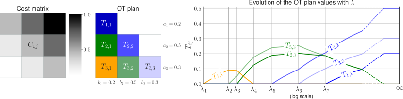
Figure 1: (Left) cost matrix $\boldsymbol{C}$ (the higher the cost, the darker the color); (middle) OT plan whose cells are color-coded with respect to the $\lambda$ values at which they are activated. The blank cells never enter the active set as the corresponding cost it too high; (right) evolution of $T_{i,j}$ when $\lambda$ increases. Note that the $x$-axis is in log scale and is discontinued between $\lambda_{7}$ and $\infty$.

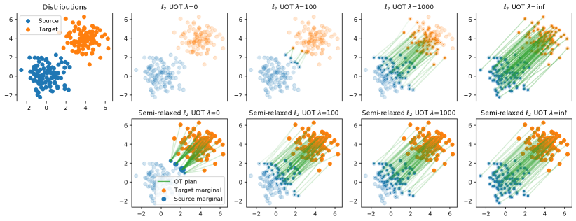
Figure 2: Regularization paths for 2D empirical distributions for $\ell_{2}$-penalized UOT (top) and semi-relaxed UOT (bottom). The OT plan is shown as green lines between the source and target samples when $T_{i,j}>0$ and the resulting marginals are shown as filled circles.

Comparison of the performances of the algorithms.

We now provide an empirical evaluation of the running times of the proposed algorithms, using 2 sets of 10-dimensional points with $n=m$ and drawn according to IID Gaussian distributions. The cost matrix $\boldsymbol{C}$ is computed using a squared $\ell_{2}$ norm. We first study the running times of the regularization path algorithm, for $n=m$ ranging from 100 to 1000, averaging the results over 5 runs, see Fig. 3 (left). We empirically observe that log-log plot is near-linear, with an empirical complexity $O(n^{3.27})$ in this example.

Using $n=m=500$, we compare the running times of the current state-of-the-art BFGS algorithm (Blondel et al., 2018) using SciPy (Virtanen et al., 2020) and those of our algorithms: the $\ell_{2}$-penalized UOT formulated as a Lasso problem (with both the Celer algorithm (Massias et al., 2018) and the coordinate descent solvers from Scikit-learn (Pedregosa et al., 2011)), the multiplicative algorithm for both the $\ell_{2}$ and the KL penalties and the regularization path algorithm (see Section A.6 of the supplemental material for more details about the solvers and their parameters). Figure 3 (middle and right) shows the average running time for all algorithms. For $\ell_{2}$-penalized UOT, we observe that, for large $\lambda$ values, the Lasso solvers are the fastest and that, whatever the value $\lambda$, BFGS is the slowest. We also notice that, for large $\lambda$, the running times for computing the path remain constant: when the last active set is found, computing the OT plan only involves a weighted sum. As for KL-penalized UOT, the BFGS algorithm is more efficient when large values of $\lambda$ are considered. One can also notice that, similarly to Sinkhorn which is fast for large regularization values, the multiplicative algorithms for both penalties are also fast for high $1/\lambda$ values.

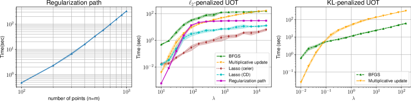
Figure 3: (Left) Running times of Alg. 1 w.r.t. the number of points; (middle) comparison of $\ell_{2}$-penalized UOT with $m=n=500$ (right) likewise for KL-penalized UOT. Dark curves (resp. shaded regions) represent average (resp. variance) values over 5 runs.

Regularization path for unbalanced domain adaptation.

We demonstrate the interest of having the entire regularization path in a classification context where some of the data collection may be polluted by outliers. We consider a setup similar to Mukherjee et al. (2020). Let the source $\boldsymbol{X}$ be a set of 400 MNIST digits sampled from the digits $0,1,2,3$ (100 points per class) and let the target $\boldsymbol{Y}$ be a set of digits $0,1$ of MNIST (LeCun et al., 2010) and of digits $8,9$ from Fashion MNIST (Xiao et al., 2017). Our setting is simple classification: we classify a sample of the target dataset by propagating

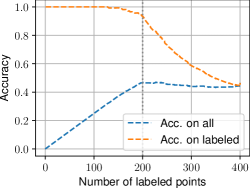
Figure 4: Evolution of the classification accuracy for the domain adaptation problem w.r.t. the number of classified points.

the label of the source sample it is the most transported to, provided that the transported mass of the target point is greater than $0.25b_{j}$. Note that similarly to Mukherjee et al. (2020) a validation set can be used here to select the best $\lambda$. Figure 4 shows the overall accuracy, defined as the number of samples that are correctly classified divided by the total number of points, and the current accuracy, which is the proportion of well-classified points among the points that are classified, i.e., that are receiving mass. One can notice that, as the number of classified points increases (with $\lambda$), the overall accuracy increases as more and more points are well classified while the current accuracy remains stable until outliers are included in the labeled set. This suggests that UOT can be used not only for classification but also as an automated outlier detection method.

5 Discussion and perspectives

We showed that UOT can be recast as a non-negative penalized linear regression problem, encouraging us to dig into this well-established field of research in order to adapt existing algorithmic solutions to the structure of the UOT problem. In this section, we discuss the relation between the proposed algorithms and classical solvers used in OT, and also investigate some research directions that can widen the scope of proposed methods.

Multiplicative algorithms for UOT.

As discussed in Section 3.1, the multiplicative updates for the KL divergence obtained from MM resemble the Sinkhorn algorithm from Chizat et al. (2018), except for the joint scaling and the weighting matrix $\exp(-\boldsymbol{C}/2)$. Interestingly, this scaling matrix also appears in the Inexact Proximal Point OT (IPOT) algorithm of Xie et al. (2020) to solve balanced OT. As a matter of fact, we show in Section A.5 of the supplementary that IPOT is a MM algorithm. The idea is to re-write the OT objective as $[\langle\boldsymbol{C},\boldsymbol{T}\rangle+\lambda D_{\varphi}(\boldsymbol{T},\boldsymbol{a}\boldsymbol{b}^{\top})]-\lambda D_{\varphi}(\boldsymbol{T},\boldsymbol{a}\boldsymbol{b}^{\top})$ and upper bound the concave term by its tangent. This further supports the interest of MM for OT and UOT, and highlight an important feature of one of our contributions: designing the first Sinkhorn-like multiplicative algorithm for UOT that can be applied when the OT plan is not entropy-regularized.

More efficient solvers.

Despite the positive experimental results of Section 4, multiplicative and regularization path algorithms can be slow, especially for large values of $\lambda$. Various accelerations can be envisaged. Regarding path algorithms, the approach of Mairal and Yu (2012) can compute a regularization path with precision $\epsilon$ in $o(1/\epsilon)$ iterations. This would lead in our setting to a full complexity of $O({mn}/{\epsilon})$ that is even interesting to approximate balanced OT. Another way to speed up computations is to use screening. In sparse regression, this consists of eliminating during optimization components that will not belong to the support of the solutions thanks to safe screening tests. Methods such as (El Ghaoui et al., 2012; Wang et al., 2015; Dantas et al., 2021) can readily be adapted to our $\ell_{2}$ or KL-penalized UOT algorithms. Finally, an other line of improvement is to consider stochastic optimization methods such as (Defazio et al., 2014). Given the particular structure of $\boldsymbol{H}$, the complexity of stochastic updates shall be small and can lead to very efficient implementations (Nesterov, 2014).

General case and entropy-regularized UOT.

Following (Frogner et al., 2015; Chizat et al., 2018; Séjourné et al., 2019), general regularized UOT can be expressed as:

$$\text{RUOT}^{\boldsymbol{\lambda}}(\boldsymbol{a},\boldsymbol{b})=\min_{\boldsymbol{T}\geq 0}\quad\langle\boldsymbol{C},\boldsymbol{T}\rangle+\lambda_{1}D_{\varphi}(\boldsymbol{T}\mathds{1}_{m},\boldsymbol{a})+\lambda_{2}D_{\varphi}(\boldsymbol{T}^{\top}\mathds{1}_{n},\boldsymbol{b})+\lambda_{\text{reg}}D_{\varphi}(\boldsymbol{T},\boldsymbol{a}\boldsymbol{b}^{\top}).$$ (13)

As it turns out, this general problem involving different regularization weights $(\lambda_{1},\lambda_{2},\lambda_{\text{reg}})$ can easily be addressed in our framework as well using two simple tricks. The first one consists of absorbing the regularization weights into the divergences. Indeed, many divergences are homogeneous, i.e., satisfy a relation of the form $\lambda D_{\varphi}(\mathbf{x}|\mathbf{y})=D_{\varphi}(\lambda^{\alpha}\mathbf{x}|\lambda^{\alpha}\mathbf{y})$ where $\alpha$ is divergence-specific. This holds in particular for the KL divergence ($\alpha=1$) and the squared $\ell_{2}$ norm ($\alpha=1/2$). The second one consists of complementing $\boldsymbol{H}$ and $\boldsymbol{y}$ with suitable terms to account for the regularization term. In the end, we may re-write Eq. (13) into Eq. (3) with $\lambda=1$, $\boldsymbol{H}=[\lambda_{1}^{\alpha}\boldsymbol{H}_{r}^{\top},\lambda_{2}^{\alpha}\boldsymbol{H}_{c}^{\top},\lambda^{\alpha}_{\text{reg}}\mathbf{I}]^{\top}$ and $\boldsymbol{y}^{\top}=[\lambda^{\alpha}_{1}\boldsymbol{a}^{\top},\lambda^{\alpha}_{2}\boldsymbol{b}^{\top},\lambda^{\alpha}_{\text{reg}}\text{vec}(\boldsymbol{a}\boldsymbol{b}^{\top})^{\top}]$. In particular, we obtain the following multiplicative update in the case of entropy-regularized KL-penalized UOT:

$$\boldsymbol{T}^{(k+1)}=\text{diag}\left(\frac{\boldsymbol{a}}{\boldsymbol{T}^{(k)}\mathds{1}_{m}}\right)^{\frac{\lambda_{1}}{\lambda_{\text{all}}}}\left(\left(\boldsymbol{T}^{(k)}\right)^{\frac{\lambda_{1}+\lambda_{2}}{\lambda_{\text{all}}}}\odot\boldsymbol{K}\right)\text{diag}\left(\frac{\boldsymbol{b}}{{\boldsymbol{T}^{(k)\top}}\mathds{1}_{n}}\right)^{\frac{\lambda_{2}}{\lambda_{\text{all}}}}$$ (14)

where $\boldsymbol{K}=\left(\boldsymbol{a}\boldsymbol{b}^{\top}\right)^{\frac{\lambda_{\text{reg}}}{\lambda_{\text{all}}}}\odot\text{exp}\left(-\frac{1}{\lambda_{\text{all}}}\boldsymbol{C}\right)$ and $\lambda_{\text{all}}=\lambda_{1}+\lambda_{2}+\lambda_{\text{reg}}$. This multiplicative update is slightly more complex than the Sinkhorn algorithms of Frogner et al. (2015); Chizat et al. (2018) and as such, it might have limited practical interest but is conceptually interesting and novel. Note that balanced UOT as of Eq. (2) is simply obtained with $\lambda_{\text{reg}}=0$.

Non-linear UOT.

Finally, we discuss how our proposed reformulation of UOT can accommodate non-linear variants in which the linear term $\langle\boldsymbol{C},\boldsymbol{T}\rangle$ is replaced by a sparsity/robustness-promoting term, leading to problems of the form

$$\text{NLUOT}^{\boldsymbol{\lambda}}(\boldsymbol{a},\boldsymbol{b})=\min_{\boldsymbol{T}\geq 0}\quad\sum_{i,j}g(C_{i,j}T_{i,j})+\lambda_{1}D_{\varphi}(\boldsymbol{T}\mathds{1}_{m},\boldsymbol{a})+\lambda_{2}D_{\varphi}(\boldsymbol{T}^{\top}\mathds{1}_{n},\boldsymbol{b})$$ (15)

where $g(\cdot)$ is a usually concave function, see, e.g., (Candes et al., 2008; Gasso et al., 2009). Our MM setting can readily accommodate such a formulation by majorizing the concave terms by their tangent. The non-linearity may improve robustness w.r.t outliers and better model realistic OT problems. For instance, in real life, the costs of transporting some goods between two places can be nonlinear due to economies of scale.

Broad and potential negative societal impact.

The contributions in this paper are methodological and focus on a reformulation of a fundamental OT problem and adapting existing algorithms to solve it. In this sense, we bring more efficient solvers that run on GPU but this computational advantage can be counterbalanced by the possibility that it brings to be applied on larger datasets. The application of OT in domain adaptation has shown that it can be used to infer labels on samples/individuals when no labels are available, suggesting a capacity for violating user privacy. A potential application of UOT is the case where two datasets of users acquired by different methods contain some shared users. UOT can be used here to find correspondences between the users in the two datasets and also identify unique users in each dataset (those that do not receive mass).

6 Conclusion

In this paper, we reformulate the UOT problem as a non-negative penalized linear regression, allowing us to propose two new classes of algorithms. We first derive multiplicative algorithms for both KL and $\ell_{2}$-penalized UOT, providing numerical solutions that are fast and easy to implement. For the specific case of $\ell_{2}$-penalized UOT, we provide the first regularization path algorithm that computes the whole set of solutions for all the regularization parameter values. We finally build on the extensive literature in inverse problem and NMF to draw some fruitful perspectives on even more efficient algorithmic solutions or the definition of new OT problems.

Appendix A Supplementary material

A.1 Design of $\boldsymbol{H}$, $\boldsymbol{H}_{r}$ and $\boldsymbol{H}_{c}$

In this section, we detail how we build the design matrix $\boldsymbol{H}$ in problem (3). By setting $\lambda=\lambda_{1}=\lambda_{2}$, Eq. (2) can be reformulated as

$$\text{UOT}^{\lambda}(\boldsymbol{a},\boldsymbol{b})=\min_{\boldsymbol{T}\geq 0}\quad\langle\boldsymbol{C},\boldsymbol{T}\rangle+\lambda D_{\varphi}\left(\begin{bmatrix}\boldsymbol{T}\mathds{1}_{m}\\ \boldsymbol{T}^{\top}\mathds{1}_{n}\end{bmatrix},\begin{bmatrix}\boldsymbol{a}\\ \boldsymbol{b}\end{bmatrix}\right)$$ (16)

because the divergence $D_{\varphi}$ is separable. Note that both $\boldsymbol{T}\mathds{1}_{m}$ and $\boldsymbol{T}^{\top}\mathds{1}_{n}$ are linear operations. It means that we can vectorize the matrix $\boldsymbol{t}=\text{vec}(\boldsymbol{T})=[T_{1,1},T_{1,2},\dots T_{n,m-1},T_{n,m}]^{\top}$ such that:

$$\begin{bmatrix}\boldsymbol{T}\mathds{1}_{m}\\ \boldsymbol{T}^{\top}\mathds{1}_{n}\end{bmatrix}=\boldsymbol{H}\boldsymbol{t}\qquad\text{where}\qquad\boldsymbol{H}=\begin{bmatrix}\boldsymbol{H}_{r}\\ \boldsymbol{H}_{c}\end{bmatrix}.$$ (17)

The matrix $\boldsymbol{H}_{r}\in\mathbb{R}_{n\times nm}$ that performs the sum over the rows of $\boldsymbol{T}$ is given by

$$\boldsymbol{H}_{r}=\begin{bmatrix}1&\dots&1&0&\dots&0&\dots&0&\dots&0\\ 0&\dots&0&1&\dots&1&\dots&0&\dots&0\\ \ldots&\ldots&\ldots&\ldots&\ldots&\ldots&\ldots&\ldots&\ldots&\ldots\\ 0&\dots&0&0&\dots&0&\dots&1&\dots&1\\ \end{bmatrix}$$ (18)

and can be implemented in Python with $\boldsymbol{H}_{r}=$ np.repeat(np.eye(n),m). In a similar fashion, the matrix $\boldsymbol{H}_{c}$ that performs the sum across columns of $\boldsymbol{T}$ is a $m\times nm$ array defined as

$$\boldsymbol{H}_{c}=\begin{bmatrix}\boldsymbol{I}_{m}&\boldsymbol{I}_{m}&\dots&\boldsymbol{I}_{m}\end{bmatrix}$$ (19)

and can be implemented in Python using $\boldsymbol{H}_{c}=$ np.tile(np.eye(m),n).

Useful identities.

From the previous definitions, we have that

$$\boldsymbol{H}^{\top}\boldsymbol{y}=\boldsymbol{H}_{r}^{\top}\boldsymbol{a}+\boldsymbol{H}_{c}^{\top}\boldsymbol{b}=\text{vec}(\boldsymbol{a}\mathds{1}_{m}^{\top}+\mathds{1}_{n}\boldsymbol{b}^{\top})=\begin{bmatrix}a_{1}+b_{1}\\ a_{1}+b_{2}\\ \ldots\\ a_{n}+b_{m-1}\\ a_{n}+b_{m}\end{bmatrix}.$$ (20)

We have $\boldsymbol{H}^{\top}\boldsymbol{H}=\boldsymbol{H}_{r}^{\top}\boldsymbol{H}_{r}+\boldsymbol{H}_{c}^{\top}\boldsymbol{H}_{c}$, of size $nm\times nm$. $\boldsymbol{H}_{r}^{\top}\boldsymbol{H}_{r}$ is a block-diagonal matrix with $n$ blocks of size $m\times m$ filled with ones. $\boldsymbol{H}_{r}^{\top}\boldsymbol{H}_{r}$ can be implemented in Python with np.tile(np.eye(m),(n,m)). $\boldsymbol{H}_{c}^{\top}\boldsymbol{H}_{c}$ is a block matrix with blocks of $\boldsymbol{I}_{m}$, and can be implemented in Python with np.tile(np.eye(m), (n,n)). Multiplying $\boldsymbol{H}^{\top}\boldsymbol{H}$ by a vector, e.g. $\boldsymbol{t}$, results in $\boldsymbol{H}^{\top}\boldsymbol{H}\boldsymbol{t}=\text{vec}(\boldsymbol{T}\mathds{1}_{m}\mathds{1}_{m}^{\top}+\mathds{1}_{n}\mathds{1}_{n}^{\top}\boldsymbol{T})$.

A.2 Details of MM algorithms

The objective function $F_{\lambda}(\boldsymbol{t})$ defined by Eq. (3) can be re-written as:

$$F_{\lambda}(\boldsymbol{t})=\sum_{i}\varphi(\sum_{j}H_{i,j}t_{j})+\sum_{j}\left[\frac{c_{j}}{\lambda}-\sum_{i}H_{i,j}\varphi^{\prime}(y_{i})\right]t_{j}.$$ (21)

Applying Jensen inequality to the first term like explained in Section 3.1 directly leads to the expression of $G_{\lambda}(\boldsymbol{t},\tilde{\boldsymbol{t}})$ given by Eq. (4). The auxiliary function is separable and convex. Given $\tilde{\boldsymbol{t}}={\boldsymbol{t}}^{(k)}$, the next iterate $\boldsymbol{t}^{(k+1)}$ can be computed by cancelling the partial derivative $\nabla_{t_{q}}G_{\lambda}(\boldsymbol{t},\boldsymbol{t}^{(k)})$, $q=1,\ldots,nm$, or setting $t_{q}$ to zero if the solution is negative in order to satisfy the non-negative constraint (note that this is not a heuristic but what the KKT conditions dictate). Cancelling the partial derivative w.r.t. $t_{q}$ is equivalent to solving

$$\sum_{i}H_{i,q}\varphi^{\prime}\left(\frac{t_{q}}{t^{(k)}_{q}}[\boldsymbol{H}\boldsymbol{t}^{(k)}]_{i}\right)=\sum_{i}H_{i,q}\varphi^{\prime}(y_{i})-\frac{c_{q}}{\lambda}$$ (22)

w.r.t. $t_{q}$. We address this univariate problem for the $\ell_{2}$ and KL-penalties next.

Squared $\ell_{2}$ penalty.

In that case we have $\varphi(x)=\frac{x^{2}}{2}$, $\varphi^{\prime}(x)=x$ and we obtain

$$t_{q}^{(k+1)}=t^{(k)}_{q}\,\frac{\max\left(0,[\boldsymbol{H}^{\top}\boldsymbol{y}]_{q}-\frac{1}{\lambda}c_{q}\right)}{[\boldsymbol{H}^{\top}\boldsymbol{H}\boldsymbol{t}^{(k)}]_{q}}.$$ (23)

Recall that $\boldsymbol{t}$ is a vector form of the OT plan $\boldsymbol{T}$, and assume that $t_{q}$ corresponds to the entry $T_{i,j}$. $\boldsymbol{H}^{\top}\boldsymbol{y}$ is a $nm$-dimensional vector with elements $a_{i}+b_{j}$, see Eq. (20). Furthermore, we have $\boldsymbol{H}\boldsymbol{t}=\begin{bmatrix}\boldsymbol{T}\mathds{1}_{m}\\ \boldsymbol{T}^{\top}\mathds{1}_{n}\end{bmatrix}$ thanks to Eq. (17). Therefore, we can establish the following update in $T_{i,j}$

$$T_{i,j}^{(k+1)}=T_{i,j}^{(k)}\,\frac{\max\left(0,a_{i}+b_{j}-\frac{1}{\lambda}c_{i,j}\right)}{[\boldsymbol{T}^{(k)}\mathds{1}_{m}]_{i}+[{\boldsymbol{T}^{(k)}}^{\top}\mathds{1}_{n}]_{j}}$$ (24)

with matrix form given by Eq. (7).

KL penalty.

In this case we have $\varphi(x)=x\log x-x$, $\varphi^{\prime}(x)=\log x$ and we obtain

$$t^{(k+1)}_{q} =t_{q}^{(k)}\exp\left(\frac{1}{\sum_{q}H_{i,q}}\left(\sum_{i}H_{i,q}\log\frac{y_{i}}{[\boldsymbol{H}\boldsymbol{t}^{(k)}]_{i}}-\frac{c_{q}}{\lambda}\right)\right)$$ (25)

$$=t^{(k)}_{q}\,\exp\left(\frac{\left[\boldsymbol{H}^{\top}\log(\boldsymbol{y})-\boldsymbol{H}^{\top}\log\left(\boldsymbol{H}\boldsymbol{t}^{(k)}\right)\right]_{q}-\frac{1}{\lambda}c_{q}}{\left[\boldsymbol{H}^{\top}\mathds{1}\right]_{q}}\right).$$ (26)

Using the results of Section A.1 like in the $\ell_{2}$ case, we obtain the following update

$$T_{i,j}^{(k+1)} = \left(\frac{a_{i}}{[\boldsymbol{T}^{(k)}\mathds{1}_{m}]_{i}}\right)^{1/2}\,T_{i,j}^{(k)}\exp\left(-\frac{c_{i,j}}{2\lambda}\right)\,\left(\frac{b_{j}}{[{\boldsymbol{T}^{(k)}}^{\top}\mathds{1}_{n}]_{j}}\right)^{1/2}$$

with matrix form given by Eq. (6).

Alternative multiplicative update for the $\ell_{2}$-penalty.

Another possible approach is to use a quadratic majorization of the linear term $\boldsymbol{c}^{\top}\boldsymbol{t}$ to bypass the thresholding operation like in (Hoyer, 2002; Yang and Oja, 2011), leading to:

$$\boldsymbol{T}^{(k+1)}=\boldsymbol{T}^{(k)}\odot\frac{\boldsymbol{a}\mathds{1}_{m}^{\top}+\mathds{1}_{n}\boldsymbol{b}^{\top}}{\boldsymbol{T}^{(k)}\mathbf{O}_{m}+\mathbf{O}_{n}\boldsymbol{T}^{(k)}+\frac{1}{2\lambda}\boldsymbol{C}}\quad\text{with}\quad\mathbf{O}_{\ell}=\mathds{1}_{\ell}\mathds{1}_{\ell}^{\top}.$$ (27)

However we found update (7) more useful in our case, thanks to the thresholding operation that locates true zeros from start.

Alternative derivation of MM algorithms.

The reformulation of UOT as a non-negative penalized linear regression problem comes very handy because it offers a novel interpretation of UOT and the possibility of using some of the many existing algorithms for the latter problem, such as LARS-based algorithm for path computation. However, we want to point out that we may also derive MM algorithms directly from Eq. (2). Let us write

$$F_{\lambda}(\boldsymbol{T}) =\langle\boldsymbol{C},\boldsymbol{T}\rangle+\lambda_{1}D_{\varphi}(\boldsymbol{T}\mathds{1}_{m},\boldsymbol{a})+\lambda_{2}D_{\varphi}(\boldsymbol{T}^{\top}\mathds{1}_{n},\boldsymbol{b})$$ (28)

$$=\sum_{ij}C_{i,j}T_{i,j}+\lambda_{1}\sum_{i}d_{\varphi}(\sum\nolimits_{j}T_{i,j},a_{i})+\lambda_{2}\sum_{j}d_{\varphi}(\sum\nolimits_{i}T_{i,j},b_{j})$$ (29)

(Note that we have $F_{\lambda}(\boldsymbol{T})=F_{\lambda}(\boldsymbol{t})$, slightly abusing notations). Let $\tilde{\boldsymbol{T}}$ be a current estimate of $\boldsymbol{T}$. We wish to compute an auxiliary function $G_{\lambda}(\boldsymbol{T},\tilde{\boldsymbol{T}})$ for $F_{\lambda}(\boldsymbol{T})$. Let us denote

$$\tilde{a}_{i} =\sum_{j}\tilde{T}_{i,j}\quad\text{(the $i^{th}$ approximate row marginal)}$$ (30)

$$\tilde{b}_{j} =\sum_{i}\tilde{T}_{i,j}\quad\text{(the $j^{th}$ approximate column marginal)}$$ (31)

$$\tilde{\alpha}_{i,j} =\frac{\tilde{T}_{i,j}}{\tilde{a}_{i}}\quad\ \ \quad\text{such that }\sum_{j}\tilde{\alpha}_{i,j}=1$$ (32)

$$\tilde{\beta}_{i,j} =\frac{\tilde{T}_{i,j}}{\tilde{b}_{j}}\quad\ \ \quad\text{such that }\sum_{i}\tilde{\beta}_{i,j}=1$$ (33)

By convexity of $d_{\varphi}(x,y)$ w.r.t $x$, we have

$$d_{\varphi}\left(\sum_{j}T_{i,j},a_{i}\right) \leq\sum_{j}\tilde{\alpha}_{i,j}\,d_{\varphi}\left(\frac{T_{i,j}}{\tilde{\alpha}_{i,j}},a_{i}\right),$$ (34)

$$d_{\varphi}\left(\sum_{i}T_{i,j},b_{j}\right) \leq\sum_{i}\tilde{\beta}_{i,j}\,d_{\varphi}\left(\frac{T_{i,j}}{\tilde{\beta}_{i,j}},b_{j}\right).$$ (35)

The inequalities are tight when $\tilde{\boldsymbol{T}}=\boldsymbol{T}$. Plugging the latter inequalities into Eq. (29), we obtain the following auxiliary function:

$$G_{\lambda}(\boldsymbol{T}|\tilde{\boldsymbol{T}})=\sum_{ij}\left[C_{i,j}T_{i,j}+\lambda_{1}\tilde{\alpha}_{i,j}\,d_{\varphi}\left(\frac{T_{i,j}}{\tilde{\alpha}_{i,j}},a_{i}\right)+\lambda_{2}\tilde{\beta}_{i,j}\,d_{\varphi}\left(\frac{T_{i,j}}{\tilde{\beta}_{i,j}},b_{j}\right)\right].$$ (36)

$G_{\lambda}(\boldsymbol{T}|\tilde{\boldsymbol{T}})$ is essentially the matrix form of $G_{\lambda}(\boldsymbol{t}|\tilde{\boldsymbol{t}})$, with partial derivative given by:

$$\nabla_{T_{i,j}}G_{\lambda}(\boldsymbol{T}|\tilde{\boldsymbol{T}})=C_{i,j}+\lambda_{1}d_{\varphi}^{\prime}\left(\tilde{a}_{i}\frac{T_{i,j}}{\tilde{T}_{i,j}},a_{i}\right)+\lambda_{2}d_{\varphi}^{\prime}\left(\tilde{b}_{j}\frac{T_{i,j}}{\tilde{T}_{i,j}},b_{j}\right).$$ (37)

Using $d^{\prime}_{\varphi}(x,y)=\varphi^{\prime}(x)-\varphi^{\prime}(y)$ and either $\varphi^{\prime}(x)=x$ ($\ell_{2}$-penalized UOT) or $\varphi^{\prime}(x)=\log x$ (KL-penalized UOT), we easily retrieve Eq. (24) and Eq. (A.2) when $\lambda_{1}=\lambda_{2}$, or Eq. (14) in the general case (with here $\lambda_{\text{reg}}=0$).

A.3 Details of the UOT path computation

Matrices and vectors on the active set $\mathcal{A}$.

Recall that $\boldsymbol{m}_{\mathcal{A}}$, $\boldsymbol{c}_{\mathcal{A}}$ and $\boldsymbol{t}_{\mathcal{A}}$ are sub-vectors of $\boldsymbol{m}$, $\boldsymbol{c}$ and $\boldsymbol{T}$ corresponding to indices in $\mathcal{A}$. $\boldsymbol{H}_{\mathcal{A}}$ is a matrix of dimension $(|i|+|j|)\times|\mathcal{A}|$, where $|i|$ and $|j|$ are respectively the number of distinct rows $i$ and columns $j$ that belong to the transport plan for a given active set $\mathcal{A}$. $\boldsymbol{H}_{\mathcal{A}}$ is built by keeping only the rows of $\boldsymbol{H}_{r}$ such that the element $i$ is present in the active set (the latter matrix being denoted $[\boldsymbol{H}_{r}]_{\mathcal{A}}$), the rows of $\boldsymbol{H}_{c}$ such that the element $j$ is present in the active set (denoted $[\boldsymbol{H}_{c}]_{\mathcal{A}}$), and keeping the columns such that element $(i,j)\in\mathcal{A}$ (up to vectorization).

Update $(\boldsymbol{H}_{\mathcal{A}}^{\top}\boldsymbol{H}_{\mathcal{A}})^{-1}$ from $(\boldsymbol{H}_{\mathcal{A}_{k}}^{\top}\boldsymbol{H}_{\mathcal{A}_{k}})^{-1}$ using the Schur complement.

Algorithm 1 involves the computation, at each iteration, of the inverse matrix $(\boldsymbol{H}_{\mathcal{A}}^{\top}\boldsymbol{H}_{\mathcal{A}})^{-1}$. The computational burden can be alleviated by using the Schur complement of the matrix in order to compute $(\boldsymbol{H}_{\mathcal{A}}^{\top}\boldsymbol{H}_{\mathcal{A}})^{-1}$ from its value at the previous iteration $(\boldsymbol{H}_{\mathcal{A}_{k}}^{\top}\boldsymbol{H}_{\mathcal{A}_{k}})^{-1}$. Let us denote $\boldsymbol{B}_{\mathcal{A}}=(\boldsymbol{H}_{\mathcal{A}}^{\top}\boldsymbol{H}_{\mathcal{A}})$ and $\boldsymbol{B}_{\mathcal{A}_{k}}=(\boldsymbol{H}_{\mathcal{A}_{k}}^{\top}\boldsymbol{H}_{\mathcal{A}_{k}})$. Two cases may arise:

• One component $q$ is added to the active set $\mathcal{A}=\mathcal{A}_{k+1}=\mathcal{A}_{k}\cup q$. In that case, we have:

  $$\boldsymbol{B}^{-1}_{\mathcal{A}}=\begin{bmatrix}\boldsymbol{B}^{-1}_{\mathcal{A}_{k}}+\boldsymbol{B}^{-1}_{\mathcal{A}_{k}}b_{\mathcal{A},q}S^{-1}b_{q,\mathcal{A}}\boldsymbol{B}^{-1}_{\mathcal{A}_{k}}&-\boldsymbol{B}^{-1}_{\mathcal{A}_{k}}b_{\mathcal{A},q}S^{-1}\\ -S^{-1}b_{{q},\mathcal{A}}\boldsymbol{B}^{-1}_{\mathcal{A}}&S^{-1}\end{bmatrix}$$ (38)

  where $b_{q,\mathcal{A}}$ is the last column of matrix $\boldsymbol{B}_{\mathcal{A}}$, $b_{\mathcal{A},q}$ its last row and $S=2-b_{q,\mathcal{A}}{{}^{\top}}\boldsymbol{B}^{-1}_{\mathcal{A}_{k}}b_{\mathcal{A},q}$ is a scalar.

• One component $q$ is removed from the active set $\mathcal{A}=\mathcal{A}_{k}\backslash q$. In that case, we get:

  $$\boldsymbol{B}^{-1}_{\mathcal{A}}=\boldsymbol{B}^{-1}_{\mathcal{A}_{k}\backslash q}-\dfrac{b^{-1}_{\mathcal{A}\backslash q,q}b^{-1}_{q,\mathcal{A}\backslash q}}{b^{-1}_{q,q}}$$ (39)

  with $\boldsymbol{B}^{-1}_{\mathcal{A}\backslash q}$ being the matrix $\boldsymbol{B}^{-1}_{\mathcal{A}}$ deprived from its row and column corresponding to the component $q$. The vector $b^{-1}_{\mathcal{A}_{k}\backslash q,q}$ represents the column of the $\boldsymbol{B}^{-1}_{\mathcal{A}}$ matrix corresponding to element $i$ while $b^{-1}_{q,\mathcal{A}\backslash q}$ stands for the corresponding row. Finally $b^{-1}_{q,q}$ is the component of $\boldsymbol{B}^{-1}_{\mathcal{A}}$ corresponding to the component $q$.

A.4 Details of the regularization path formulation for semi-relaxed UOT

Semi-relaxed $\ell_{2}$-penalized UOT.

We start by recalling the formulation of the semi-relaxed $\ell_{2}$-penalized UOT problem:

$$\text{SROT}^{\boldsymbol{\lambda}}(\boldsymbol{a},\boldsymbol{b})=\min_{\boldsymbol{T}\geq 0,\boldsymbol{H}_{c}\boldsymbol{t}=\boldsymbol{b}}\,\,\langle\boldsymbol{C},\boldsymbol{T}\rangle+\lambda\|\boldsymbol{T}\mathds{1}_{m}-\boldsymbol{a}\|^{2}.$$

From Eq. (12), the corresponding Lagrangian writes:

$${L}_{\lambda}(\boldsymbol{t},\boldsymbol{\gamma})=\frac{1}{\lambda}\boldsymbol{c}^{\top}\boldsymbol{t}+{\frac{1}{2}}(\boldsymbol{H}_{r}\boldsymbol{t}-\boldsymbol{a})^{\top}(\boldsymbol{H}_{r}\boldsymbol{t}-\boldsymbol{a})+(\boldsymbol{H}_{c}\boldsymbol{t}-\boldsymbol{b})^{\top}\boldsymbol{u}-\boldsymbol{\gamma}^{\top}\boldsymbol{t}$$ (40)

with $\boldsymbol{u}\in\mathbb{R}^{m}$ the Lagrange parameters associated to the $m$ equality constraints and $\boldsymbol{\gamma}\geq 0$ the Lagrange parameters related to the non-negativity constraints. We recall the KKT optimality conditions, which state that i) $\nabla_{\boldsymbol{t}}{L}_{\lambda}=\frac{1}{\lambda}\boldsymbol{c}+\boldsymbol{H}_{r}^{\top}\boldsymbol{H}_{r}\boldsymbol{t}-\boldsymbol{H}_{r}^{\top}\boldsymbol{a}+\boldsymbol{H}_{c}^{\top}\boldsymbol{u}-\boldsymbol{\gamma}=0$ (stationary condition), ii) $\boldsymbol{\gamma}\odot\boldsymbol{t}=0$ (complementary condition), and iii) $\boldsymbol{\gamma}\geq 0$ and $\boldsymbol{H}_{c}\boldsymbol{t}-\boldsymbol{b}=\boldsymbol{0}$ (feasibility) from which we may derive the path computation. We recall that $\odot$ stands for point-wise multiplication.

Piecewise linearity of the path.

Let us suppose that, at step $k$, we know the current active set $\mathcal{A}=\mathcal{A}_{k}$ and we look for $\boldsymbol{t}_{\mathcal{A}}^{\lambda}$ and $\boldsymbol{u}^{\lambda}$. Because of the complementary condition, we have $\boldsymbol{\gamma}_{\mathcal{A}}=\boldsymbol{0}$. Hence the stationnarity condition on the active set can be rewritten as, with $\lambda=\lambda_{k}+\epsilon$ and $\epsilon$ small enough

$$\begin{cases}[\boldsymbol{H}_{r}^{\top}]_{\mathcal{A}}[\boldsymbol{H}_{r}]_{\mathcal{A}}\boldsymbol{t}^{\lambda}_{\mathcal{A}}+[\boldsymbol{H}_{c}^{\top}]_{\mathcal{A}}\boldsymbol{u}^{\lambda}&=[\boldsymbol{H}_{r}^{\top}]_{\mathcal{A}}\boldsymbol{a}_{\mathcal{A}}-\frac{1}{\lambda}\boldsymbol{c}_{\mathcal{A}}\\ [\boldsymbol{H}_{c}]_{\mathcal{A}}\boldsymbol{t}^{\lambda}_{\mathcal{A}}&=\boldsymbol{b}_{\mathcal{A}}\end{cases}$$ (41)

or equivalently, at each iteration, the following linear system should be solved:

$$\underbrace{\begin{pmatrix}[\boldsymbol{H}_{r}^{\top}]_{\mathcal{A}}[\boldsymbol{H}_{r}]_{\mathcal{A}}&[\boldsymbol{H}_{c}^{\top}]_{\mathcal{A}}\\ [\boldsymbol{H}_{c}]_{\mathcal{A}}&\boldsymbol{0}\end{pmatrix}}_{{\boldsymbol{K}}_{\mathcal{A}}}\begin{pmatrix}\boldsymbol{t}^{\lambda}_{\mathcal{A}}\\ \boldsymbol{u}^{\lambda}\end{pmatrix}=-\frac{1}{\lambda}\underbrace{\begin{pmatrix}\boldsymbol{c}_{\mathcal{A}}\\ \boldsymbol{0}\end{pmatrix}}_{\boldsymbol{\gamma}_{\mathcal{A}}}+\underbrace{\begin{pmatrix}[\boldsymbol{H}_{r}^{\top}]_{\mathcal{A}}\boldsymbol{a}_{\mathcal{A}}\\ \boldsymbol{b}\end{pmatrix}}_{\boldsymbol{\beta}_{\mathcal{A}}}.$$ (42)

We then have

$$\begin{pmatrix}\boldsymbol{t}^{\lambda}_{\mathcal{A}}\\ \boldsymbol{u}^{\lambda}\end{pmatrix}=-\frac{1}{\lambda}\boldsymbol{K}_{\mathcal{A}}^{-1}\boldsymbol{\gamma}_{\mathcal{A}}+\boldsymbol{K}_{\mathcal{A}}^{-1}{\boldsymbol{\beta}_{\mathcal{A}}}.$$ (43)

We now denote $\tilde{\boldsymbol{c}}_{\mathcal{A}}=\boldsymbol{K}_{\mathcal{A}}^{-1}\boldsymbol{\gamma}_{\mathcal{A}}$ and its sub-vectors $\tilde{\boldsymbol{c}}_{\mathcal{A}}^{\boldsymbol{a}}$ and $\tilde{\boldsymbol{c}}_{\mathcal{A}}^{\boldsymbol{b}}$ that respectively contains the $|\mathcal{A}|$ first rows and $m$ last rows of $\tilde{\boldsymbol{c}}_{\mathcal{A}}$. We also denote $\tilde{\boldsymbol{m}}_{\mathcal{A}}=\boldsymbol{K}_{\mathcal{A}}^{-1}{\boldsymbol{\beta}_{\mathcal{A}}}$ and its sub-vectors $\tilde{\boldsymbol{m}}_{\mathcal{A}}^{\boldsymbol{a}}$ and $\tilde{\boldsymbol{m}}_{\mathcal{A}}^{\boldsymbol{b}}$ in the same fashion. We then have

$$\begin{cases}\boldsymbol{t}^{\lambda}_{\mathcal{A}}=-\frac{1}{\lambda}\tilde{\boldsymbol{c}}_{\mathcal{A}}^{\boldsymbol{a}}+\tilde{\boldsymbol{m}}_{\mathcal{A}}^{\boldsymbol{a}}\\ \boldsymbol{u}^{\lambda}=-\frac{1}{\lambda}\tilde{\boldsymbol{c}}_{\mathcal{A}}^{\boldsymbol{b}}+\tilde{\boldsymbol{m}}_{\mathcal{A}}^{\boldsymbol{b}}\\ \end{cases}$$ (44)

We again notice the piecewise linearity (as a function of ${1}/{\lambda}$) of the path when the active set $\mathcal{A}$ is fixed.

Computation of $\lambda^{k+1}$ given $\lambda^{k}$.

Given a current solution at iteration $k$ $(\lambda_{k},\boldsymbol{t}^{\lambda_{k}})$, we increase the $\epsilon$ value in $\lambda=\lambda_{k}+\epsilon$ until one of the following case arises.

$\bullet$ Inside the active set, the positivity constraint on $\boldsymbol{t}_{\mathcal{A}}^{\lambda}$ may be violated, corresponding to the case

$$\tilde{\boldsymbol{m}}_{\mathcal{A}}^{\boldsymbol{a}}=\frac{1}{\lambda}\tilde{\boldsymbol{c}}_{\mathcal{A}}^{\boldsymbol{a}} \Rightarrow \lambda_{r}=\min_{>\lambda_{k}}\left(\frac{\tilde{\boldsymbol{c}}_{\mathcal{A}}^{\boldsymbol{a}}}{\tilde{\boldsymbol{m}}_{\mathcal{A}}^{\boldsymbol{a}}}\right)$$ (45)

where $\min_{>\lambda_{k}}$ denotes the smallest value in $\frac{\tilde{\boldsymbol{c}}_{\mathcal{A}}^{\boldsymbol{a}}}{\tilde{\boldsymbol{m}}_{\mathcal{A}}^{\boldsymbol{a}}}$ greater that $\lambda_{k}$.

$\bullet$ Outside the active set, the positivity constraint of the KKT may be violated. The stationarity condition outside the active set $\bar{\mathcal{A}}$ can be rewritten, by injecting the solution of Eq. (44):

$$\frac{1}{\lambda}\boldsymbol{c}_{\bar{\mathcal{A}}}+\big{[}\boldsymbol{H}_{r}^{\top}(\boldsymbol{H}_{r}(-\frac{1}{\lambda}\tilde{\boldsymbol{c}}^{\boldsymbol{a}}+\tilde{\boldsymbol{m}}^{\boldsymbol{a}})-\boldsymbol{a})\big{]}_{\bar{\mathcal{A}}}+\big{[}\boldsymbol{H}_{c}^{\top}(-\frac{1}{\lambda}\tilde{\boldsymbol{c}}^{\boldsymbol{b}}+\tilde{\boldsymbol{m}}^{\boldsymbol{b}})\big{]}_{\bar{\mathcal{A}}}-\boldsymbol{\gamma}_{\bar{\mathcal{A}}}=0$$ (46)

$$\frac{1}{\lambda}\boldsymbol{c}_{\bar{\mathcal{A}}}+\Big{[}\boldsymbol{H}^{\top}\boldsymbol{H}\big{(}\tilde{\boldsymbol{m}}+\frac{1}{\lambda}\tilde{\boldsymbol{c}}\big{)}\Big{]}_{\bar{\mathcal{A}}}-\boldsymbol{m}_{\bar{\mathcal{A}}}=\boldsymbol{\gamma}_{\bar{\mathcal{A}}} \Rightarrow \lambda_{a}=\min_{>\lambda_{k}}\left(\dfrac{\boldsymbol{c}_{\bar{\mathcal{A}}}-\big{[}\boldsymbol{H}^{\top}\boldsymbol{H}\tilde{\boldsymbol{c}}\big{]}_{\bar{\mathcal{A}}}}{\boldsymbol{m}_{\bar{\mathcal{A}}}-\big{[}\boldsymbol{H}^{\top}\boldsymbol{H}\tilde{\boldsymbol{m}}\big{]}_{\bar{\mathcal{A}}}}\right)$$ (47)

The active set changes only if there exists a component $i$ outside the current active set such that $\gamma_{i}\geq 0$. Hence we write:

$$\frac{1}{\lambda}\boldsymbol{c}_{\bar{\mathcal{A}}}-\frac{1}{\lambda}\big{[}\boldsymbol{H}_{r}^{\top}\boldsymbol{H}_{r}\tilde{\boldsymbol{c}}^{\boldsymbol{a}}+\boldsymbol{H}_{c}^{\top}\tilde{\boldsymbol{c}}^{\boldsymbol{b}}\big{]}_{\bar{\mathcal{A}}}+\big{[}\boldsymbol{H}_{r}^{\top}\boldsymbol{H}_{r}\tilde{\boldsymbol{m}}^{\boldsymbol{a}}-\boldsymbol{H}_{r}^{\top}\boldsymbol{a}+\boldsymbol{H}_{c}^{\top}\tilde{\boldsymbol{m}}^{\boldsymbol{b}}\big{]}_{\bar{\mathcal{A}}}\geq 0$$ (48)

$${\lambda_{a}}=\min_{>\lambda_{k}}\dfrac{\boldsymbol{c}_{\bar{\mathcal{A}}}-\big{[}\boldsymbol{H}_{r}^{\top}\boldsymbol{H}_{r}\tilde{\boldsymbol{c}}^{\boldsymbol{a}}+\boldsymbol{H}_{c}^{\top}\tilde{\boldsymbol{c}}^{\boldsymbol{b}}\big{]}_{\bar{\mathcal{A}}}}{\big{[}2\boldsymbol{H}_{r}^{\top}\boldsymbol{a}-\boldsymbol{H}_{r}^{\top}\boldsymbol{H}_{r}\tilde{\boldsymbol{m}}^{\boldsymbol{a}}-\boldsymbol{H}_{c}^{\top}\tilde{\boldsymbol{m}}^{\boldsymbol{b}}\big{]}_{\bar{\mathcal{A}}}}$$ (49)

Note that this last equation is very similar to the one we obtain for $\ell_{2}$-penalized UOT, except that vectors $\tilde{\boldsymbol{m}}$ and $\tilde{\boldsymbol{c}}$ are split in 2 parts, depending on if we consider the rows (that can be unbalanced) or the columns (that should strictly respect the marginal constraint). Also note that the Schur complement applies to the update of $\boldsymbol{K}_{\mathcal{A}}^{-1}$ in order to decrease the computational burden.

A.5 IPOT is a MM algorithm

Herein we discuss the relation between the Inexact Proximal Point OT (IPOT) algorithm of Xie et al. (2020) and MM. First note that IPOT aims at the balanced OT problem (1). This is equivalent to solving

$$\min_{\boldsymbol{T}\geq 0,\boldsymbol{T}\mathds{1}_{m}=\boldsymbol{a},\boldsymbol{T}^{\top}\mathds{1}_{n}=\boldsymbol{b}}\langle\boldsymbol{C},\boldsymbol{T}\rangle\quad+\lambda\sum_{i,j}T_{i,j}\log(T_{i,j})-\lambda\sum_{i,j}T_{i,j}\log(T_{i,j})$$ (50)

where one adds and removes the entropy regularization of $\boldsymbol{T}$. A simple algorithm can be devised by upper bounding the concave term by its tangent at $\boldsymbol{T}^{(k)}$ leading to the new problem

$$\min_{\boldsymbol{T}\geq 0,\boldsymbol{T}\mathds{1}_{m}=\boldsymbol{a},\boldsymbol{T}^{\top}\mathds{1}_{n}=\boldsymbol{b}}\langle\boldsymbol{T},\boldsymbol{C}\rangle+\lambda\sum_{i,j}T_{i,j}\log(T_{i,j})-\lambda\langle\boldsymbol{T},\log\left(\boldsymbol{T}^{(k)}\right)+1\rangle$$ (51)

where the log is taken component-wise. Note that the constant $1$ in the scalar product can be removed since $\sum_{i,j}T_{i,j}$ is constant and does not influence the solution. Problem (51) can be solved using classical Sinkhorn iterations with a cost matrix $\tilde{\boldsymbol{C}}=\boldsymbol{C}-\lambda\log(\boldsymbol{T}^{(k)})$. This corresponds to using the kernel matrix

$$\tilde{\boldsymbol{K}}=\exp\left(-\frac{1}{\lambda}(\boldsymbol{C}-\lambda\log\left(\boldsymbol{T}^{(k)}\right)\right)=\exp\left(-\frac{1}{\lambda}\boldsymbol{C}\right)\odot\boldsymbol{T}^{(k)},$$ (52)

as presented in (Xie et al., 2020, Algorithm 1). Hence IPOT can be interpreted as MM. Note that the point-wise product between a kernel matrix and the estimate $\boldsymbol{T}^{(k)}$ appears also in our multiplicative updates (6) and (14) with however a different scaling parameter.

A.6 Details about the experiments

We run the experiments on a Mac mini 2020 personal computer, with M1 chip and 16GB of RAM. All the experiments can be re-run thanks to the paper companion code. We compare the following algorithms provided by the following solvers:

• the “L-BFGS-B” method of SciPy, in which we provide the function to minimize and its associated Jacobian (either for KL or $\ell_{2}$-penalized UOT),

• the Lasso algorithms Celer and of Scikit-learn,

• the regularization path algorithm introduced in the paper,

• the multiplicative updates introduced in the paper.

We use the same stopping criteria for all the algorithms (not to mention the regularization path algorithm that provides an exact solution), except for $\ell_{2}$-penalized UOT that necessitates a smaller tolerance to converge to the correct values, especially for large values of $\lambda$.

Regarding Figure 3, we draw 5 realizations of two random 2 Gaussian samples of 10-dimensional $n=m$ points with different means and variances.

References

- Arjovsky et al. (2017) Arjovsky, M., S. Chintala, and L. Bottou (2017). Wasserstein Generative Adversarial Networks. In International Conference on Machine Learning, Volume 70, pp. 214–223.
- Benamou (2003) Benamou, J.-D. (2003). Numerical resolution of an “unbalanced” mass transport problem. ESAIM: Mathematical Modelling and Numerical Analysis 37(5), 851–868.
- Blondel et al. (2018) Blondel, M., V. Seguy, and A. Rolet (2018). Smooth and Sparse Optimal Transport. In International Conference on Artificial Intelligence and Statistics, pp. 880–889.
- Bonneel and Coeurjolly (2019) Bonneel, N. and D. Coeurjolly (2019). SPOT: Sliced Partial Optimal Transport. ACM Transactions on Graphics (SIGGRAPH) 38(4).
- Byrd et al. (1995) Byrd, R. H., P. Lu, J. Nocedal, and C. Zhu (1995). A Limited Memory Algorithm for Bound Constrained Optimization. SIAM Journal on Scientific Computing 16(5), 1190–1208.
- Caffarelli and McCann (2010) Caffarelli, L. A. and R. J. McCann (2010). Free boundaries in Optimal Transport and Monge-Ampère obstacle problems. Annals of Mathematics 171(2), 673–730.
- Candes et al. (2008) Candes, E. J., M. B. Wakin, and S. P. Boyd (2008). Enhancing Sparsity by Reweighted Minimization. Journal of Fourier analysis and applications 14(5-6), 877–905.
- Chizat et al. (2018) Chizat, L., G. Peyré, B. Schmitzer, and F.-X. Vialard (2018). Scaling algorithms for Unbalanced Optimal Transport problems. Mathematics of Computation 87(314), 2563–2609.
- Courty et al. (2017) Courty, N., R. Flamary, D. Tuia, and A. Rakotomamonjy (2017). Optimal Transport for Domain Adaptation. IEEE Transactions on Pattern Analysis and Machine Intelligence 39(9), 1853–1865.
- Cuturi (2013) Cuturi, M. (2013). Sinkhorn distances: Lightspeed computation of Optimal Transport. Advances in Neural Information Processing Sytems 26, 2292–2300.
- Dantas et al. (2021) Dantas, C. F., E. Soubies, and C. Févotte (2021). Safe Screening for Sparse Regression with the Kullback-Leibler Divergence. In IEEE International Conference on Acoustics, Speech and Signal Processing, pp. 5544–5548.
- De Pierro (1993) De Pierro, A. R. (1993). On the relation between the ISRA and the EM algorithm for positron emission tomography. IEEE transactions on Medical Imaging 12(2), 328–333.
- Defazio et al. (2014) Defazio, A., F. Bach, and S. Lacoste-Julien (2014). SAGA: A fast incremental gradient method with support for non-strongly convex composite objectives. In Advances in Neural Information Processing Systems.
- Dhillon and Sra (2005) Dhillon, I. S. and S. Sra (2005). Generalized nonnegative matrix approximations with Bregman divergences. In Advances in Neural Information Processing Systems, Volume 18.
- Efron et al. (2004) Efron, B., T. Hastie, I. Johnstone, and R. Tibshirani (2004). Least Angle Regression. Annals of statistics 32(2), 407–499.
- El Ghaoui et al. (2012) El Ghaoui, L., V. Viallon, and T. Rabbani (2012). Safe Feature Elimination for the LASSO and Sparse Supervised Learning Problems. Pacific Journal of Optimization 8(667–698).
- Févotte and Idier (2011) Févotte, C. and J. Idier (2011). Algorithms for nonnegative matrix factorization with the -divergence. Neural computation 23(9), 2421–2456.
- Figalli (2010) Figalli, A. (2010). The Optimal Partial Transport Problem. Archive for Rational Mechanics and Analysis 195(2), 533–560.
- Frogner et al. (2015) Frogner, C., C. Zhang, H. Mobahi, M. Araya, and T. A. Poggio (2015). Learning with a Wasserstein Loss. In Advances in Neural Information Processing System, pp. 2053–2061.
- Gasso et al. (2009) Gasso, G., A. Rakotomamonjy, and S. Canu (2009). Recovering sparse signals with a certain family of nonconvex penalties and DC programming. IEEE Transactions on Signal Processing 57(12), 4686–4698.
- Hastie et al. (2004) Hastie, T., S. Rosset, R. Tibshirani, and J. Zhu (2004). The entire regularization path for the Support Vector Machine. Journal of Machine Learning Research 5, 1391–1415.
- Ho et al. (2017) Ho, N., X. L. Nguyen, M. Yurochkin, H. H. Bui, V. Huynh, and D. Phung (2017). Multilevel Clustering via Wasserstein Means. In International Conference on Machine Learning, Volume 70, pp. 1501–1509.
- Hoyer (2002) Hoyer, P. O. (2002). Non-negative sparse coding. In IEEE Workshop on Neural Networks for Signal Processing, pp. 557–565.
- Hunter and Lange (2004) Hunter, D. R. and K. Lange (2004). A tutorial on MM algorithms. The American Statistician 58(1), 30–37.
- Kantorovich (1942) Kantorovich, L. (1942). On the transfer of masses (in Russian). Doklady Akademii Nauk 2, 227–229.
- Kusner et al. (2015) Kusner, M., Y. Sun, N. Kolkin, and K. Weinberger (2015). From word embeddings to document distances. In International Conference on Machine Learning, pp. 957–966.
- LeCun et al. (2010) LeCun, Y., C. Cortes, and C. Burges (2010). MNIST handwritten digit database. ATT Labs [Online]. Available: http://yann.lecun.com/exdb/mnist.
- Lee and Seung (1999) Lee, D. and H. Seung (1999). Learning the parts of objects by non-negative matrix factorization. Nature 401(6755), 788–791.
- Lee and Seung (2001) Lee, D. and H. Seung (2001). Algorithms for Non-negative Matrix Factorization. In Advances in Neural Information Processing Sytems, Volume 13.
- Liero et al. (2018) Liero, M., A. Mielke, and G. Savaré (2018). Optimal entropy-transport problems and a new Hellinger-Kantorovich distance between positive measures. Inventiones mathematicae 211(3), 969–1117.
- Mairal and Yu (2012) Mairal, J. and B. Yu (2012). Complexity Analysis of the Lasso Regularization Path. In International Conference on Machine Learning, pp. 1835–1842.
- Maretic et al. (2019) Maretic, H. P., M. E. Gheche, G. Chierchia, and P. Frossard (2019). GOT: An Optimal Transport framework for Graph comparison. In Advances In Neural Information Processing Systems, Volume 32.
- Massias et al. (2018) Massias, M., A. Gramfort, and J. Salmon (2018). Celer: a Fast Solver for the Lasso with Dual Extrapolation. In International Conference on Machine Learning, Volume 80, pp. 3321–3330.
- Mukherjee et al. (2020) Mukherjee, D., A. Guha, J. Solomon, Y. Sun, and M. Yurochkin (2020). Outlier-Robust Optimal Transport. Technical report, arXiv preprint arXiv:2012.07363.
- Nesterov (2014) Nesterov, Y. (2014). Subgradient methods for huge-scale optimization problems. Mathematical Programming 146(1), 275–297.
- Pedregosa et al. (2011) Pedregosa, F., G. Varoquaux, A. Gramfort, V. Michel, B. Thirion, O. Grisel, M. Blondel, P. Prettenhofer, R. Weiss, V. Dubourg, et al. (2011). Scikit-learn: Machine learning in Python. Journal of Machine Learning Research 12, 2825–2830.
- Rabin et al. (2014) Rabin, J., S. Ferradans, and N. Papadakis (2014). Adaptive color transfer with relaxed optimal transport. In IEEE International Conference on Image Processing, pp. 4852–4856.
- Richardson (1972) Richardson, W. H. (1972). Bayesian-based iterative method of image restoration. JoSA 62(1), 55–59.
- Sato et al. (2020) Sato, R., M. Yamada, and H. Kashima (2020). Fast Unbalanced Optimal Transport on a Tree. In Advances in Neural Information Processing Systems, Volume 33.
- Séjourné et al. (2019) Séjourné, T., J. Feydy, F.-X. Vialard, A. Trouvé, and G. Peyré (2019). Sinkhorn divergences for Unbalanced Optimal Transport. arXiv preprint arXiv:1910.12958.
- Sinkhorn and Knopp (1967) Sinkhorn, R. and P. Knopp (1967). Concerning nonnegative matrices and doubly stochastic matrices. Pacific Journal of Mathematics 21(2), 343–348.
- Sun et al. (2017) Sun, Y., P. Babu, and D. P. Palomar (2017). Majorization-minimization algorithms in signal processing, communications, and machine learning. IEEE Transactions on Signal Processing 65(3), 794–816.
- Thibault et al. (2021) Thibault, A., L. Chizat, C. Dossal, and N. Papadakis (2021). Overrelaxed Sinkhorn–Knopp Algorithm for Regularized Optimal Transport. Algorithms 14(5), 143.
- Vayer et al. (2019) Vayer, T., L. Chapel, R. Flamary, R. Tavenard, and N. Courty (2019). Optimal transport for structured data with application on graphs. In International Conference on Machine Learning, pp. 6275–6284.
- Villani (2009) Villani, C. (2009). Optimal Transport: Old and New, Volume 338. Springer Berlin Heidelberg.
- Virtanen et al. (2020) Virtanen, P., R. Gommers, T. E. Oliphant, M. Haberland, T. Reddy, D. Cournapeau, E. Burovski, P. Peterson, W. Weckesser, J. Bright, S. J. van der Walt, M. Brett, J. Wilson, K. J. Millman, N. Mayorov, A. R. J. Nelson, E. Jones, R. Kern, E. Larson, C. J. Carey, İ. Polat, Y. Feng, E. W. Moore, J. VanderPlas, D. Laxalde, J. Perktold, R. Cimrman, I. Henriksen, E. A. Quintero, C. R. Harris, A. M. Archibald, A. H. Ribeiro, F. Pedregosa, P. van Mulbregt, and SciPy 1.0 Contributors (2020). SciPy 1.0: Fundamental Algorithms for Scientific Computing in Python. Nature Methods 17, 261–272.
- Wang et al. (2015) Wang, J., P. Wonka, and J. Ye (2015). Lasso screening rules via dual polytope projection. Journal of Machine Learning Research 16(1), 1063–1101.
- Xiao et al. (2017) Xiao, H., K. Rasul, and R. Vollgraf (2017). Fashion-MNIST: a Novel Image Dataset for Benchmarking Machine Learning Algorithms.
- Xie et al. (2020) Xie, Y., X. Wang, R. Wang, and H. Zha (2020). A fast proximal point method for computing exact Wasserstein distance. In Uncertainty in Artificial Intelligence, pp. 433–453.
- Yang and Oja (2011) Yang, Z. and E. Oja (2011). Unified Development of Multiplicative Algorithms for Linear and Quadratic Nonnegative Matrix Factorization. IEEE Transactions on Neural Networks 22, 1878 – 1891.