Adversarial Semantic Hallucination for Domain Generalized Semantic Segmentation

Abstract

Convolutional neural networks typically perform poorly when the test (target domain) and training (source domain) data have significantly different distributions. While this problem can be mitigated by using the target domain data to align the source and target domain feature representations, the target domain data may be unavailable due to privacy concerns. Consequently, there is a need for methods that generalize well despite restricted access to target domain data during training. In this work, we propose an adversarial semantic hallucination approach (ASH), which combines a class-conditioned hallucination module and a semantic segmentation module. Since the segmentation performance varies across different classes, we design a semantic-conditioned style hallucination module to generate affine transformation parameters from semantic information in the segmentation probability maps of the source domain image. Unlike previous adaptation approaches, which treat all classes equally, ASH considers the class-wise differences. The segmentation module and the hallucination module compete adversarially, with the hallucination module generating increasingly “difficult” stylized images to challenge the segmentation module. In response, the segmentation module improves as it is trained with generated samples at an appropriate class-wise difficulty level. Our results on the Cityscapes and Mapillary benchmark datasets show that our method is competitive with state of the art work. Code is made available at https://github.com/gabriel-tjio/ASH.

1 Introduction

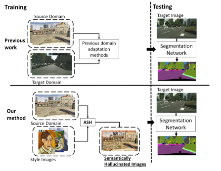
Figure 1: Illustrated summary of our proposed Adversarial Semantic Hallucination approach (ASH). Previous domain adaptation works require target domain data during training. Since target domain data are unavailable in our problem setting, we generate additional data with randomized styles via style transfer with ASH.

Semantic segmentation [2] involves classifying image pixels into a given category. While deep learning has vastly improved semantic segmentation performance, it requires large amounts of pixel-level annotated data. Pixel-level annotation is time-consuming and error-prone, making it impractical for real-life applications. For training vision systems in autonomous vehicles, synthetic data are readily available and easily labeled. However, synthetic data (source domain data) differ visually from real-world driving data (target domain data). As a result of this domain gap, models that are trained solely on synthetic data perform poorly on real-world data.

Domain adaptation methods [1, 8, 12, 19, 30, 22, 36] seek to minimize the domain gap between the source domain and target domain by utilizing unlabeled target domain data. Unfortunately, in Domain Generalization (DG) scenarios [37, 26, 5, 4], target domain data are not accessible during training. With limited access to target data, it becomes quite difficult, if not impossible, to apply previous unsupervised domain adaptation methods [1, 8, 12, 19, 30, 22, 36]. To solve this problem, hallucination-based approaches [16, 37, 20] have been proposed. These methods generate augmented images by varying texture information in the source domain images. By randomizing these domain variant features, the trained model becomes more sensitive to domain invariant features, such as shape information. The increased sensitivity to domain invariant features helps the model generalize better to the unseen target domain data. For example, Adversarial Style Mining [20] (ASM) uses a single target domain image to hallucinate additional training images. The global statistics of the single target domain image are used to adaptively stylize the source domain images. The “difficulty” of the stylized images is progressively increased via adversarial training.

Most prior works [16, 37, 20] conduct hallucination in a global manner and fail to consider the statistical differences between different classes. In real scenarios, datasets might be imbalanced because of collection and/or annotation difficulties. Consequently, classes with fewer examples are more difficult to predict accurately. For example, in the driving datasets [27, 28, 6], a larger proportion of pixels correspond to “road”, “building”, or “sky” classes compared to minority classes such as “pole” or “light”. We argue that uniformly stylizing all classes without considering their different characteristics may lead to a sub-optimal result.

Prior works, such as [18, 7], tried to address this problem by leveraging focal loss [18] or class balanced loss [7]. However, these approaches still have their limitations. Class balancing methods like focal loss [18] assume that source and target domain distributions are similar, which does not always hold true [14]. Additionally, hyperparameter selection for these methods [18, 7] is nontrivial and the hyperparameters may not be transferable between datasets.

To address these limitations, we propose a new method, Adversarial Semantic Hallucination (ASH), for domain generalized semantic segmentation. Inspired by ASM [20], we further extend it by using semantic information to guide adversarial hallucination and improve generalizability. The semantic information from the segmentation probability map is used to differentiate between classes based on their segmentation difficulty and generate transformation parameters for the style features. ASH stylizes the source domain images with these transformation parameters. Next, ASH collaborates with a discriminator in an adversarial manner by adaptively generating challenging data for training the segmentation network. With our method, the segmentation network not only becomes better at differentiating between classes, but also demonstrates good generalizability across different domains.

Our main contributions are summarized as follows:

1) We present ASH for domain generalized semantic segmentation. ASH leverages semantic information to conduct a class-conditioned stylization for source domain images, making the trained model generalize better. Unlike previous work such as ASM [20] which utilizes stylization, our method does not need any target domain data during training and thus is more practical. Additionally, our approach also considers the different characteristics between classes instead of treating them equally.

2) We conduct extensive domain generalized semantic segmentation experiments to test the efficacy of ASH, including domain generalization from GTA5 [27] or SYNTHIA datasets [28] $\rightarrow$ the Cityscapes [6] or Mapillary benchmark datasets [23]. The experimental results demonstrate the efficacy of ASH even when target data are not available during training.

2 Related Work

In this section, we briefly survey previous works that are most related to ours, including unsupervised domain adaptation and generative adversarial networks.

2.1 Unsupervised Domain Adaptation

Unsupervised domain adaptation (UDA) is a subset of transfer learning. Given labeled source data and unlabeled target data, UDA aims to train a network to achieve satisfactory performance on target domain data. Previous works [30, 8] align the feature representations of the source and target domains by minimizing the discrepancy between the two domains. Following this alignment approach, the knowledge learned from the source domain can be applied to the target domain. UDA methods can be generally divided into three categories, namely pixel-level alignment, feature-level alignment, and output-level alignment. Pixel-level domain adaptation [1] transforms the source domain images to visually mimic the target domain images. The transformed source domain images are included during training. Alternatively, target-to-source image translation has also been explored [36]. Different from these approaches, our method reduces overfitting to textural features in the source domain data instead of generating data that mimics either domain. Feature-level domain adaptation [8, 12, 19] aligns the feature representations across domains, making the feature representations extracted from the source and target domain indistinguishable. This approach has been studied for image classification [8] and semantic segmentation [19]. Output-level domain adaptation [30, 22] maximises the similarity between domains at the output level. Tsai et al. [31] and Luo et al. [21] demonstrated that output-level alignment performs better compared to feature-level alignment for semantic segmentation. Recently, source-free adaptation methods such as [17] adapt a model pretrained on source domain data to the target domain. The problem setting for such work restricts access to source domain data instead of target domain data after pretraining the model. In contrast, our method does not use target domain data during training. The work most related to our approach is ASM [20]. Luo et al. [20] aim to solve unsupervised domain adaptive semantic segmentation when limited unlabeled target data are available. Both ASM [20] and our approach utilize a style transfer strategy to generate augmented data. However, there are significant differences between the two works: (1) ASM requires target data (one single target domain image) for domain alignment. Conversely, our approach does not need any target data for training, making it more applicable for real-life scenarios. (2) ASM uses a global stylization approach. The stylized image is globally updated with the target task prediction loss on the stylized data. Consequently, pixels from different classes are uniformly stylized, which could reduce performance for the ‘harder’ classes on target domain data. In contrast, we consider the class-wise differences and utilize the semantic information for a class-conditioned process. The experimental results reported in Tables.1 and 2 demonstrate the advantages of ASH compared to ASM.

2.2 Generative Adversarial Networks (GANs)

GANs have garnered much attention since their introduction [9] and have been used in a wide range of applications, such as image generation [15] and image translation [38]. GAN architecture typically comprises of a generator-discriminator pair optimized in a min-max fashion. The generator is trained to synthesize realistic images while the discriminator is trained to distinguish between the synthesized images and the real images. Though GANs have been used for unsupervised domain adaptation [22, 1], the lack of target domain data for the domain generalization problem setting means that some modifications are required. Therefore, we train the discriminator to distinguish between segmented output from the source domain images and the randomly stylized source domain images.

Next, we apply the principle behind conditional GANs [33] for greater control over the stylization extent of the source domain image. Conditional GANs give the user additional control over the generated output via prior information to the generator. We were also further inspired by recent works [24, 34] which demonstrate prior information improves synthesized image quality. Wang et al. [34] leverage semantic information to improve output image quality during super- resolution. The probability map serves as a prior and is used as an input for spatial transformation of the image features. Similarly, Park et al. [24] condition the synthesized GAN output with semantic information during feature transformation. This enables their approach to generate realistic images, while also allowing the user to determine the content of the generated images.

We extend existing domain adaptation work by incorporating semantic information as a prior. Our ASH module is lightweight and only consists of a few convolutional layers to: 1) map the semantic information to latent space, and 2) compute the transformation coefficients for the style features. Furthermore, ASH is required only during training and therefore does not increase computation cost during inference.

3 Method

In this section, we firstly discuss our problem setting and preliminary background. We then provide the technical details for ASH.

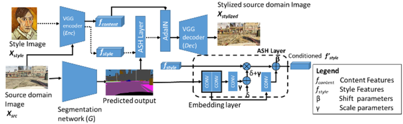
Figure 2: Illustrated workflow for generating stylized source domain images with Adversarial Semantic Hallucination (ASH). A pretrained VGG encoder extracts features from the source and style images. ASH conditions the style features with semantic information from the segmented source domain image. The semantic information is used to generate the element-wise scale and shift parameters $\boldsymbol{\gamma}$ and $\boldsymbol{\beta}$. These transformation parameters adjust the style features based on the predicted class in the segmentation output. Since the transformation parameters are only intended to perturb the style features, we include a non-zero constant $\delta$. The content features are re-normalized with the transformed style features via Adaptive Instance Normalization (AdaIN). The merged features are then decoded to output stylized source images.

3.1 Problem Setting

The problem setting for domain generalization is defined as follows: We have source domain data $\boldsymbol{X_{src}}$ with labels $\boldsymbol{Y_{src}}$ during training, but we cannot access target domain data $\boldsymbol{X_{target}}$. The source domain and target domain have different data distributions (i.e P($\boldsymbol{X_{src}}$,$\boldsymbol{Y_{src}}$) $\neq$ P($\boldsymbol{X_{target}}$,$\boldsymbol{Y_{target}}$)). Our goal is to develop a model $G$ that correctly predicts the target domain labels after training.

3.2 Preliminary background

Our method can be divided into 2 stages. In the first stage, our approach incorporates the style transfer method [13]. We augment the source domain data $\boldsymbol{X_{src}}$ by stylizing it with images from a paintings dataset $\boldsymbol{X_{sty}}$, i.e., Painter by Numbers. The style features are conditioned with semantic information obtained from the segmentation output of source domain data. In the second stage, we separately train the different components: an ASH module, a segmentation network and a discriminator.

Similar to [13], we use a pretrained VGG19 network to extract features from the source domain images and style images. We then use adaptive instance normalization [13]:

$$\text{AdaIN}(\boldsymbol{f_{src}},\boldsymbol{f_{sty}})=\sigma(\boldsymbol{f_{sty}})\left(\frac{\boldsymbol{f_{src}}-\mu(\boldsymbol{f_{src}})}{\sigma(\boldsymbol{f_{src}})}\right)+\mu(\boldsymbol{f_{sty}})$$ (1)

which re-normalizes the channel-wise mean $\mu(.)$ and variance $\sigma(.)$ of the content features (i.e source features $\boldsymbol{f_{src}}$) to match that of the style features $\boldsymbol{f_{sty}}$.

Firstly, we aim to improve the generalizability of the trained segmentation model by introducing randomized texture variations during training. At each iteration, we randomly select a style image to stylize the source image. By stylizing the source image with randomized style information, the model learns to disregard texture information.

Next, we increase the diversity of the style features by introducing orthogonal noise [35]. Orthogonal noise allows us to preserve the inner product of the style features, or its “inherent style information”, while simultaneously increasing the diversity of the style features [35]. We regularize the segmentation output with label smoothing before conditioning the style features with the ASH module.

3.3 Adversarial Semantic Hallucination

As shown in Figure 2, our framework comprises a segmentation network, a discriminator and an ASH module. The ASH module conditions the style features with semantic information from the source data segmentation output.

Prior hallucination works such as [20] conduct the stylization without considering class-wise differences, which might be sub-optimal. We take a different approach by conducting the hallucination conditioned on semantic information. The semantic information is used to compute the scale $\boldsymbol{\gamma}$ and shift $\boldsymbol{\beta}$ transformation parameters. These parameters transform the style features in latent space. Depending on the predicted class for each pixel, ASH is trained to maximize adversarial loss by assigning different scale and shift transformation parameters. We use adaptive instance normalization [13] to merge the content features with the transformed style features.

Algorithm 1 Adversarial approach for domain generalization

1:Source domain data $\boldsymbol{X_{src}}$, Source domain label $\boldsymbol{Y_{src}}$, Style image $\boldsymbol{X_{sty}}$, Segmentation network G, Discriminator D, Encoder Enc, Decoder Dec, Adversarial Semantic Hallucination ASH, Adaptive Instance Normalization (AdaIN), Number of iterations $Iter_{num}$

2:Optimized segmentation network for domain generalization

3:for $0$, …, $Iter_{num}$ do

4:   Generate source features $\boldsymbol{f_{src}}$ with pretrained encoder $Enc(\boldsymbol{X_{src}})$.

5:   Generate style features $\boldsymbol{f_{style}}$ with pretrained encoder $Enc(\boldsymbol{X_{sty}})$.

6:   Multiply style features $\boldsymbol{f_{sty}}$ with an orthogonal noise matrix $\boldsymbol{Z}$ sampled from a normal distribution

7:   Obtain scale $\boldsymbol{\gamma}$ and shift $\boldsymbol{\beta}$ coefficients from segmentation output $G(\boldsymbol{X_{src}})$

8:   Generate perturbed style features $\boldsymbol{f_{sty}^{{}^{\prime}}}$ from $\boldsymbol{f_{sty}}$ with scale $\boldsymbol{\gamma}$ and shift $\boldsymbol{\beta}$ coefficients.

9:   Derive merged source features $\boldsymbol{f_{merged}}$ = AdaIN($\boldsymbol{f_{src}}$,$\boldsymbol{f_{sty}^{{}^{\prime}}}$) .

10:   Generate stylized source image $\boldsymbol{X_{stylized}}=Dec(0.5\boldsymbol{f_{merged}}+0.5\boldsymbol{f_{src}})$.

11:   Train ASH by maximizing the loss function $\mathcal{L}_{ASH}(G,D,\boldsymbol{f_{src}},\boldsymbol{f_{sty}^{{}^{\prime}}})$.

12:   Train $G$ with source domain data by minimizing segmentation loss $\mathcal{L}_{seg}(G,\boldsymbol{X_{src}},\boldsymbol{Y_{src}})$.

13:   Train $G$ with stylized source domain data by minimizing adversarial loss. $\mathcal{L}_{adv}(G,D,\boldsymbol{X_{stylized}},\text{ASH})$.

14:   Train $D$ by minimizing adversarial loss $\mathcal{L}_{adv}(G,D,\boldsymbol{X_{stylized}},\boldsymbol{X_{src}},\text{ASH})$.

15:end for

We generate the scale $\boldsymbol{\gamma}$ and shift $\boldsymbol{\beta}$ coefficients from the segmentation output $G(\boldsymbol{X_{src}})$, as shown in the following equation:

$$\boldsymbol{\gamma},\boldsymbol{\beta}=\text{ASH}(G(\boldsymbol{X_{src}}))$$ (2)

We then perturb the style features $\boldsymbol{f_{sty}}$ to generate perturbed style features $\boldsymbol{f_{sty}^{{}^{\prime}}}$:

$$\boldsymbol{f_{sty}^{{}^{\prime}}}=\boldsymbol{Z}\cdot\boldsymbol{f_{sty}}\cdot(\boldsymbol{\gamma}+\delta)+\boldsymbol{\beta}$$ (3)

where $\delta$ is a constant perturbation value . We use a nonzero value to preserve the style features during stylization. $\boldsymbol{Z}$ is the orthogonal noise. We generate the stylized source domain images $\boldsymbol{X_{stylized}}$ with the following equation:

$$\boldsymbol{X_{stylized}}=Dec(0.5\boldsymbol{f_{src}}+0.5\text{AdaIN}(\boldsymbol{f_{src}},\boldsymbol{f_{sty}^{{}^{\prime}}}))))$$ (4)

where $Dec$ is a pretrained decoder, AdaIN is the adaptive instance normalization equation defined in equation 1. Adversarial loss is given by the following equation:

$$\mathcal{L}_{adv}(G,D,\text{ASH})= -E[\log(D(G(\boldsymbol{X_{src}})))]$$ (5)

$$-E[\log(1-D(G(\boldsymbol{X_{stylized}})))]$$

where $G$ is the segmentation network and $D$ is the discriminator. We optimize the ASH module by minimizing the following loss function:

$$\mathcal{L}_{ASH}(G,D,\boldsymbol{f_{src}},\boldsymbol{f_{style}^{{}^{\prime}}})=$$ (6)

$$-\mathcal{L}_{adv}(G,D,\text{ASH})$$

$$-\mathcal{L}_{c}(\boldsymbol{f_{src}},\text{AdaIN}(\boldsymbol{f_{src}},\boldsymbol{f_{sty}^{{}^{\prime}}}))$$

$$+\mathcal{L}_{s1}(\boldsymbol{f_{sty}^{{}^{\prime}}},\text{AdaIN}(\boldsymbol{f_{src}},\boldsymbol{f_{sty}^{{}^{\prime}}}))$$

$$-\mathcal{L}_{s2}(\boldsymbol{f_{src}},\text{AdaIN}(\boldsymbol{f_{src}},\boldsymbol{f_{sty}^{{}^{\prime}}}))\vspace{-0.5cm}$$

We use the formula for content $\mathcal{L}_{c}$ and style $\mathcal{L}_{s}$ loss as defined in [13]. $\mathcal{L}_{c}$, $\mathcal{L}_{s1}$ and $\mathcal{L}_{s2}$ are described as:

$$\mathcal{L}_{c}=\left\lVert\boldsymbol{f_{src}}-\text{AdaIN}(\boldsymbol{f_{src}},\boldsymbol{f_{sty}^{{}^{\prime}}})\right\rVert_{2}$$ (7)

$$\mathcal{L}_{s1}=\left\lVert\mu(\boldsymbol{f_{style}^{{}^{\prime}}})-\mu(\text{AdaIN}(\boldsymbol{f_{src}},\boldsymbol{f_{sty}^{{}^{\prime}}}))\right\rVert_{2}$$ (8)

$$\mathcal{L}_{s2}=\left\lVert\mu(\boldsymbol{f_{src}^{{}^{\prime}}})-\mu(\text{AdaIN}(\boldsymbol{f_{src}},\boldsymbol{f_{sty}^{{}^{\prime}}}))\right\rVert_{2}$$ (9)

$\mathcal{L}_{c}$ is minimized to preserve content information from the source image. We minimize $\mathcal{L}_{s1}$ to maximize the style information retained from the style images. $\mathcal{L}_{s2}$ is maximized to minimize the style information retained from the source image.

The segmentation network $G$ [22] is trained to minimize segmentation loss $\mathcal{L}_{seg}$ and adversarial loss $\mathcal{L}_{adv}$. The discriminator network $D$ is trained to maximize adversarial loss $\mathcal{L}_{adv}$. Both loss functions are based on the formulation from [22]. Segmentation loss $\mathcal{L}_{seg}$ is derived from computing the cross entropy loss for the segmentation output.

The training workflow is summarized in Algorithm 1. The weights for the pretrained encoder and decoder that are used during stylization are not updated during training. We only need the segmentation network for evaluation, neither the ASH module nor discriminator are required after training.

4 Experiments

In this section, we discuss the experimental details. We first describe the datasets utilized in this work in Section. 4.1. Secondly, we provide implementation details in Section 4.2. We provide details for all experimental results in Section 4.3 - 4.5. Section 4.3 presents the performance of our approach on the benchmark datasets and compares it with the state of the art unsupervised domain adaptation and domain generalization methods. Section 4.4 shows the effect of the hyperparameters on segmentation performance. Section 4.5 shows the ablation studies.

4.1 Datasets

We use the synthetic datasets GTA5 [27], SYNTHIA [28] as source domains, the real-world driving datasets Cityscapes [6] and Mapillary [23] as the target domain. GTA5 [27] has 24,966 images with resolution $1914\times 1052$ pixels, while SYNTHIA [28] has 9,400 images with $1280\times 760$ pixels. Models are trained on the labeled source domain images and evaluated on the Cityscapes and Mapillary validation set. Similar to [13], we use a paintings dataset (Painter by Numbers, which is derived from WikiArt) to provide 45,203 style images.

GTA5 $\rightarrow$ Cityscapes
	Year	Arch.	road	side.	buil.	wall	fence	pole	light	sign	vege.	terr.	sky	pers.	rider	car	truck	bus	train	motor	bike	mIoU
Advent [32]	2019	R	83.00	1.80	72.00	8.20	3.60	16.20	22.90	9.80	79.30	17.10	75.70	35.10	15.80	70.90	30.90	35.30	0.00	16.40	24.90	32.60
MaxSquare [3]	2019	R	76.80	14.20	77.00	18.80	14.10	14.50	30.30	18.00	79.30	11.70	70.50	53.00	24.20	68.70	25.30	14.00	1.30	20.60	25.50	34.60
CLAN [22]	2019	R	87.20	20.10	77.90	25.60	19.70	23.00	30.40	22.50	76.80	25.20	76.20	55.10	28.10	82.70	30.70	36.90	0.80	26.00	17.10	40.10
ASM[20]	2020	R	56.20	0.00	7.00	0.60	1.00	0.30	0.70	0.60	13.80	0.10	0.01	0.08	0.04	1.20	0.50	0.70	0.20	0.00	0.00	4.40
Domain Rand.[37]	2019	R	-	-	-	-	-	-	-	-	-	-	-	-	-	-	-	-	-	-	-	42.53
ASH (Ours)	2021	R	88.30	19.80	78.80	23.60	19.50	24.40	30.30	24.70	79.10	27.00	74.40	56.40	27.90	83.40	36.40	38.40	0.80	22.50	29.80	41.30
ASH (Uni.Sem.Info.)	2021	R	87.40	17.00	77.70	20.60	17.80	22.80	30.10	24.50	78.70	24.60	72.70	55.60	26.50	81.50	32.20	37.70	1.10	21.70	20.50	39.50
GTA5 $\rightarrow$ Mapillary
ASH	2021	R	81.47	21.22	74.37	21.78	24.97	32.82	34.3	28.18	73.02	38.14	90.68	56.21	38.64	73.63	37.39	37.27	7.51	35.9	36.79	44.44
Domain Rand.[37]	2019	R	-	-	-	-	-	-	-	-	-	-	-	-	-	-	-	-	-	-	-	38.05

Table 1: Segmentation performance of Deeplab-v2 with Resnet-101 backbone trained on GTA5, tested on Cityscapes and Mapillary. “ASH Uni.Sem.Info”- ASH with uniform class-wise probability map (identical values across all classes and pixels).

SYNTHIA $\rightarrow$ Cityscapes
	Year	Arch.	road	side.	buil.	light	sign	vege.	sky	pers.	rider	car	bus	motor	bike	mIoU	mIoU16
Advent [32]	2019	R	72.30	30.70	65.20	4.10	5.40	58.20	77.20	50.40	10.10	70.00	13.20	4.00	27.90	37.60	31.80
MaxSquare [3]	2019	R	57.80	23.19	73.63	8.37	11.66	73.84	81.92	56.68	20.73	52.18	14.71	8.37	39.18	40.17	34.96
CLAN [22]	2019	R	63.90	25.90	72.10	14.30	12.00	72.50	78.70	52.70	14.50	62.20	25.10	10.40	26.50	40.90	34.90
ASM [20]	2020	R	75.40	18.50	66.60	0.10	0.80	67.00	77.80	15.60	0.50	11.40	1.30	0.03	0.20	25.80	21.60
Domain Rand.[37]	2019	R	-	-	-	-	-	-	-	-	-	-	-	-	-	-	37.58
ASH	2021	R	70.20	27.90	75.40	16.00	15.20	74.20	80.10	55.00	20.40	71.10	29.60	10.90	38.20	44.90	38.69
ASH (Segmentation Loss)	2021	R	68.10	25.43	74.98	12.93	12.98	73.29	78.81	55.36	22.13	69.77	30.45	9.60	36.75	43.89	37.88
ASH (Ground truth)	2021	R	63.37	23.93	7.30	14.58	11.09	77.92	80.60	54.77	13.42	68.34	26.49	12.71	24.73	42.25	36.29

Table 2: Segmentation performance of Deeplab-v2 with Resnet-101 backbone SYNTHIA→Cityscapes. ASH (Ground truth) refers to stylized images conditioned with ground truth labels. “ASH (segmentation loss)” refers to ASH trained with segmentation loss for the stylized images $\mathcal{L}_{seg}(G,\boldsymbol{X_{sty}},\boldsymbol{Y_{src}})$.

Method	Venue	mIoU16
Advent [32]	CVPR 2019	29.33
CLAN [22]	CVPR 2019	36.91
Domain Rand.[37]	ICCV 2019	34.12
ASH	-	38.34
ASH (segmentation loss)	-	38.54
ASH ($\delta$=0)	-	37.61

Table 3: Mean IoU (16 classes) for the segmentation network (Deeplab-v2 with Resnet-101 backbone) SYNTHIA →Mapillary.

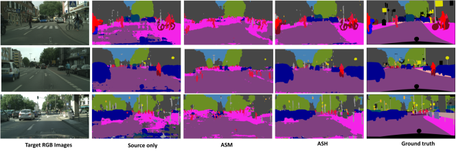
Figure 3: Qualitative comparison of segmentation output for SYNTHIA → Cityscapes. For each target domain image, we show the corresponding results for “Source only”, “ASM” Adversarial Style Mining [20], “ASH”(our proposed method) and the ground truth labels.

4.2 Implementation details

We implement our approach with the PyTorch library [25] on a single 16GB Quadro RTX 5000. The GTA5 images are resized to $1280\times 720$ pixels and the SYNTHIA images are resized to $1280\times 760$ pixels. We use the Deeplab-v2 segmentation network [2] with ResNet-101 [10] backbone pretrained on the ImageNet dataset [29]. The discriminator network architecture is similar to the one used in [22].

We use stochastic gradient descent (SGD) to optimize the segmentation network (Deeplab-v2) and ASH module. Adam is used to optimize the discriminator network. All optimizers have a momentum of 0.9. The initial learning rate for the segmentation network and the discriminator network is $2.5\times 10^{-4}$ and $1.0\times 10^{-4}$. We train the network for 100,000 iterations.

4.3 Experimental studies

We compare our method with 5 representative methods [3, 22, 32, 20, 37] and present the results in Tables 1 and 2. [3, 22, 32] are UDA approaches where target domain data are available during training; [20] aims to align domains with limited target domain data and [37] is a domain generalization approach. Maximum Squares Loss [3] improves upon semi-supervised learning by preventing easier classes from dominating training, CLAN [22] seeks to reduce the difference between learned feature representations from the source and target domain, while ADVENT [32] aims to reduce the prediction uncertainty for target domain data. ASM [20] generates additional training data from a target domain image under one shot UDA approach. Domain randomization [37] stylizes multiple instances of a source domain image with style images obtained from ImageNet [29] for each iteration and performs pyramidal pooling on the extracted features to maintain feature consistency between the different stylized instances.

We also compare ASH with Domain Randomization (DR) [37], and report the results in Tables 1, 2 and 3. ASH outperformed DR on SYNTHIA→Cityscapes and SYNTHIA/GTA5→Mapillary. There exist key differences between ASH and DR. DR generates 15 stylized images for each source domain image, while ASH only stylizes a single source domain image once per training iteration. Furthermore, DR performs spatial pyramid pooling on the extracted features. All these aspects increase computational requirements. With much less computational cost, our approach still achieves comparable results for GTA5→Cityscapes and superior performance for GTA5→Mapillary (Table 1). For a direct comparison with SFTGAN [34] we show results for ASH ($\delta=0$) (Table 3). In contrast with our approach, Wang et al. [34] did not include a nonzero value during feature transformation in their work on super-resolution. We observe that performance decreases when $\delta=0$. The decreased performance may be caused by loss of some style features when scale perturbation $\gamma=0$. Furthermore, Figure 4 shows that $\gamma=0$ for some classes. The lack of stylization for these classes may have worsened performance, indicating the necessity of a nonzero $\delta$ value during stylization.
We also trained ASH with additional supervision (ASH segmentation loss) and show the results in Tables 2 and 3. We observe comparable performance with ASH. Next, we trained a ASH model that receives uniform semantic information across all classes (ASH Uni.Sem.Info) (Table 1). The reduced performance highlight the importance of semantic information. Finally, we conditioned the stylization with ground truth instead of segmentation output (Table 2). Segmentation performance was lowered, suggesting that the segmentation output contains useful information absent in the ground truth, which is unsurprising given the regularizing effect of soft labels during model distillation [11].

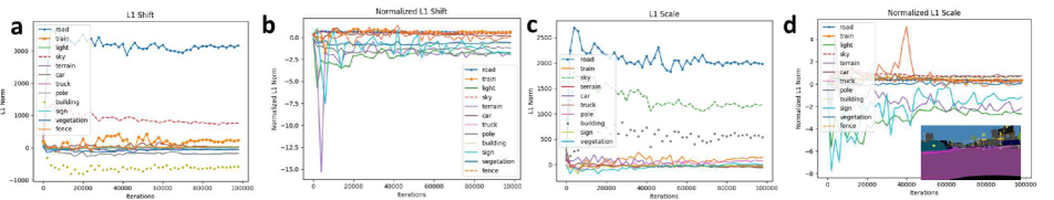
Figure 4: Plots of L1 norm of shift $\boldsymbol{\beta}$ and scale $\boldsymbol{\gamma}$ coefficients versus number of iterations during training. a) Plot of L1 shift coefficients $\boldsymbol{\beta}$; b) Plot of L1 shift coefficients with class-wise normalization $\boldsymbol{\beta}$ c) Plot of L1 scale coefficients $\boldsymbol{\gamma}$; d) Plot of L1 scale coefficients $\boldsymbol{\gamma}$ with class-wise normalization. Corresponding semantic label image(inset).

$\lambda$	0.1	0.01	0.001	0.0001
mIoU	33.33	35.41	38.69	37.53

Table 4: Segmentation performance for the segmentation task SYNTHIA→Cityscapes with varying adversarial loss hyperparameter magnitudes.

4.4 Hyperparameter evaluation

In Table 4, we evaluate the effect of varying the adversarial loss weights on segmentation performance. Our results show that performance decreases much more when weights are increased than when the weights are decreased.

Baseline	Stylization	Orthogonal	ASH	mIoU
		Noise
✓				36.6
✓	✓			40.1
✓	✓	✓		40.8
✓	✓	✓	✓	41.3

Table 5: Ablation study for GTA5→Cityscapes. The baseline approach is the CLAN [22] method trained on source domain data. Stylization refers to the model trained with additional stylized data, ASH is our proposed method.

$\mathcal{L}_{c}$	$\mathcal{L}_{s1}$	$\mathcal{L}_{s2}$	mIoU
			36.91
✓			37.13
✓	✓		38.27
✓	✓	✓	38.69

Table 6: Ablation study for the ASH sublosses from equation 6, SYNTHIA→Cityscapes

4.5 Ablation study

In Table 5, we compare our methods with CLAN as the baseline method. Training with stylized images improves segmentation performance on target domain data. Since stylization varies texture information, there is less overfitting to these domain variant features. This improves the generalizability of the trained model. Adding orthogonal noise to the style features improves performance, which could be caused by the increased diversity of the style features. In Table 6, we evaluate the effect of the different adversarial sublosses. While omitting any of the sublosses worsens performance, $\mathcal{L}_{s1}$ appears to have the greatest effect. Since $\mathcal{L}_{s1}$ determines the amount of style information retained from $X_{sty}$, this suggests that the degree of stylization greatly influences generalization performance.

5 Discussion

5.1 Scale and shift coefficients

We further investigate the scale and shift coefficients by class (Figure 4). We calculate the L1 norm of all the scale and shift coefficients for each class in a single source image. This was obtained from the change in the L1 norm after zeroing the contribution of that class.
As expected, majority classes contribute more to the scale and shift coefficients than minority classes. In particular, “road” and “sky” classes have a larger effect on scale and shift coefficients compared to other classes such as “pole” and “light” (Figure 4 a,c). Since larger scale and shift coefficients are proportionate to the change in the style features, this suggests that “road” and “sky” classes undergo a larger degree of stylization compared to “pole” and “light” classes.
These observations lead us to suggest that the ASH module selectively stylizes classes that occupy a large proportion of pixels in the predicted segmentation output for a given image (e.g “road”, “sky”). Since the ASH module is optimized to generate stylized images that maximize adversarial loss, it appears that the network stylizes majority class pixels more than minority class pixels to maximize adversarial loss by increasing task difficulty.
Furthermore, several classes have negligible scale and shift coefficients. Although these classes (e.g “vegetation”, “pole”) are present in the segmentation output, regions corresponding to these classes do not undergo significant stylization compared to the majority classes. Classes such as “vegetation” and “pole” do not vary considerably in terms of colour information or texture. Consequently, stylizing these classes does not significantly affect the adversarial loss, which might explain the small variations in scale and shift coefficients.

5.2 Normalized scale and shift coefficients

We normalize the class-wise change in scale and shift coefficients by the number of pixels predicted for each class. This was done to provide greater clarity on the stylization for minority classes, since minority classes (e.g. “pole”, “light”) have much fewer pixels compared to majority classes (e.g. “road”, “building”).

While it may not be apparent from the plots in Figure 4 a and c, classes that occupy a smaller area in the image also undergo stylization. We observe that “road” and “building” classes have smaller absolute normalized shift and scale coefficients, while “terrain” , “light” and “sign” classes have much larger absolute normalized L1 coefficients (Figure 4 b,d). These results show that almost all classes, with the exception of classes such as ’vegetation’, do undergo stylization, though majority classes are generally stylized to a greater extent compared to miniority classes.

6 Conclusions

In this paper, we introduce the adversarial style hallucination network, which addresses the problem of adapting to an unseen target domain. By using an adversarial approach conditioned on semantic information, ASH can adaptively stylize the source domain images. Additionally, using semantic information allows ASH to account for class-wise differences during stylization instead of treating all classes equally. Experimental results demonstrate the efficacy of our proposed method, showing it to be competitive with state-of-the-art work.

7 Acknowledgements

The computational work for this article was partially performed on resources of the National Supercomputing Centre, Singapore (https://www.nscc.sg).

References

- [1] Konstantinos Bousmalis, Nathan Silberman, David Dohan, Dumitru Erhan, and Dilip Krishnan. Unsupervised pixel-level domain adaptation with generative adversarial networks. In Proceedings of the IEEE/CVF Conference on Computer Vision and Pattern Recognition (CVPR), 2017.
- [2] Liang-Chieh Chen, George Papandreou, Iasonas Kokkinos, Kevin Murphy, and Alan L. Yuille. Deeplab: Semantic image segmentation with deep convolutional nets, atrous convolution, and fully connected crfs. IEEE Transactions on Pattern Analysis and Machine Intelligence, 40(4):834–848, 2018.
- [3] Minghao Chen, Hongyang Xue, and Deng Cai. Domain adaptation for semantic segmentation with maximum squares loss. In Proceedings of the IEEE/CVF International Conference on Computer Vision (ICCV), 2019.
- [4] Wuyang Chen, Zhiding Yu, Shalini De Mello, Sifei Liu, Jose M. Alvarez, Zhangyang Wang, and Anima Anandkumar. Contrastive syn-to-real generalization. In International Conference on Learning Representations, 2021.
- [5] Sungha Choi, Sanghun Jung, Huiwon Yun, Joanne T. Kim, Seungryong Kim, and Jaegul Choo. Robustnet: Improving domain generalization in urban-scene segmentation via instance selective whitening. In Proceedings of the IEEE/CVF Conference on Computer Vision and Pattern Recognition (CVPR), 2021.
- [6] Marius Cordts, Mohamed Omran, Sebastian Ramos, Timo Rehfeld, Markus Enzweiler, Rodrigo Benenson, Uwe Franke, Stefan Roth, and Bernt Schiele. The cityscapes dataset for semantic urban scene understanding. In Proceedings of the IEEE/CVF Conference on Computer Vision and Pattern Recognition (CVPR), 2016.
- [7] Yin Cui, Menglin Jia, Tsung-Yi Lin, Yang Song, and Serge Belongie. Class-balanced loss based on effective number of samples. In Proceedings of the IEEE/CVF Conference on Computer Vision and Pattern Recognition (CVPR), 2019.
- [8] Yaroslav Ganin, Evgeniya Ustinova, Hana Ajakan, Pascal Germain, Hugo Larochelle, François Laviolette, Mario Marchand, and Victor S. Lempitsky. Domain-adversarial training of neural networks. In Domain Adaptation in Computer Vision Applications, Advances in Computer Vision and Pattern Recognition. 2017.
- [9] Ian Goodfellow, Jean Pouget-Abadie, Mehdi Mirza, Bing Xu, David Warde-Farley, Sherjil Ozair, Aaron Courville, and Yoshua Bengio. Generative adversarial nets. In Advances in Neural Information Processing Systems, volume 27, 2014.
- [10] Kaiming He, Xiangyu Zhang, Shaoqing Ren, and Jian Sun. Deep residual learning for image recognition. In 2016 IEEE Conference on Computer Vision and Pattern Recognition (CVPR), 2016.
- [11] Geoffrey Hinton, Oriol Vinyals, and Jeffrey Dean. Distilling the knowledge in a neural network. In NIPS Deep Learning and Representation Learning Workshop, 2015.
- [12] Judy Hoffman, Eric Tzeng, Taesung Park, Jun-Yan Zhu, Phillip Isola, Kate Saenko, Alexei Efros, and Trevor Darrell. CyCADA: Cycle-consistent adversarial domain adaptation. In Proceedings of the 35th International Conference on Machine Learning.
- [13] Xun Huang and Serge Belongie. Arbitrary style transfer in real-time with adaptive instance normalization. In Proceedings of the IEEE/CVF International Conference on Computer Vision (ICCV), 2017.
- [14] Muhammad Abdullah Jamal, Matthew Brown, Ming-Hsuan Yang, Liqiang Wang, and Boqing Gong. Rethinking class-balanced methods for long-tailed visual recognition from a domain adaptation perspective. In Proceedings of the IEEE/CVF Conference on Computer Vision and Pattern Recognition (CVPR), 2020.
- [15] Tero Karras, Samuli Laine, and Timo Aila. A style-based generator architecture for generative adversarial networks. In Proceedings of the IEEE/CVF Conference on Computer Vision and Pattern Recognition (CVPR), 2019.
- [16] Myeongjin Kim and Hyeran Byun. Learning texture invariant representation for domain adaptation of semantic segmentation. In Proceedings of the IEEE/CVF Conference on Computer Vision and Pattern Recognition (CVPR), 2020.
- [17] Jogendra Nath Kundu, Rahul Mysore Venkatesh, Naveen Venkat, Ambareesh Revanur, and R. Venkatesh Babu. Class-incremental domain adaptation. In Andrea Vedaldi, Horst Bischof, Thomas Brox, and Jan-Michael Frahm, editors, Proceedings of the European Conference on Computer Vision (ECCV), 2020.
- [18] Tsung-Yi Lin, Priya Goyal, Ross Girshick, Kaiming He, and Piotr Dollar. Focal loss for dense object detection. In Proceedings of the IEEE/CVF International Conference on Computer Vision (ICCV), 2017.
- [19] Yawei Luo, Ping Liu, Tao Guan, Junqing Yu, and Yi Yang. Significance-aware information bottleneck for domain adaptive semantic segmentation. In Proceedings of the IEEE/CVF International Conference on Computer Vision (ICCV), 2019.
- [20] Yawei Luo, Ping Liu, Tao Guan, Junqing Yu, and Yi Yang. Adversarial style mining for one-shot unsupervised domain adaptation. In Advances in Neural Information Processing Systems, 2020.
- [21] Yawei Luo, Ping Liu, Liang Zheng, Tao Guan, Junqing Yu, and Yi Yang. Category-level adversarial adaptation for semantic segmentation using purified features. IEEE Transactions on Pattern Analysis and Machine Intelligence, 2021.
- [22] Yawei Luo, Liang Zheng, Tao Guan, Junqing Yu, and Yi Yang. Taking a closer look at domain shift: Category-level adversaries for semantics consistent domain adaptation. In Proceedings of the IEEE/CVF Conference on Computer Vision and Pattern Recognition (CVPR), 2019.
- [23] Gerhard Neuhold, Tobias Ollmann, Samuel Rota Bulò, and Peter Kontschieder. The mapillary vistas dataset for semantic understanding of street scenes. In Proceedings of the IEEE/CVF International Conference on Computer Vision (ICCV), 2017.
- [24] Taesung Park, Ming-Yu Liu, Ting-Chun Wang, and Jun-Yan Zhu. Semantic image synthesis with spatially-adaptive normalization. In Proceedings of the IEEE/CVF Conference on Computer Vision and Pattern Recognition (CVPR), 2019.
- [25] Adam Paszke, Sam Gross, Francisco Massa, Adam Lerer, James Bradbury, Gregory Chanan, Trevor Killeen, Zeming Lin, Natalia Gimelshein, Luca Antiga, Alban Desmaison, Andreas Kopf, Edward Yang, Zachary DeVito, Martin Raison, Alykhan Tejani, Sasank Chilamkurthy, Benoit Steiner, Lu Fang, Junjie Bai, and Soumith Chintala. Pytorch: An imperative style, high-performance deep learning library. In Advances in Neural Information Processing Systems. 2019.
- [26] Duo Peng, Yinjie Lei, Lingqiao Liu, Pingping Zhang, and Jun Liu. Global and local texture randomization for synthetic-to-real semantic segmentation. IEEE Transactions on Image Processing, 30:6594–6608, 2021.
- [27] Stephan R. Richter, Vibhav Vineet, Stefan Roth, and Vladlen Koltun. Playing for data: Ground truth from computer games. In Proceedings of the European Conference on Computer Vision (ECCV), 2016.
- [28] German Ros, Laura Sellart, Joanna Materzynska, David Vazquez, and Antonio Lopez. The SYNTHIA Dataset: A large collection of synthetic images for semantic segmentation of urban scenes. In Proceedings of the IEEE/CVF Conference on Computer Vision and Pattern Recognition (CVPR), 2016.
- [29] Olga Russakovsky, Jia Deng, Hao Su, Jonathan Krause, Sanjeev Satheesh, Sean Ma, Zhiheng Huang, Andrej Karpathy, Aditya Khosla, Michael Bernstein, Alexander C. Berg, and Li Fei-Fei. ImageNet Large Scale Visual Recognition Challenge. International Journal of Computer Vision (IJCV), 2015.
- [30] Kuniaki Saito, Kohei Watanabe, Yoshitaka Ushiku, and Tatsuya Harada. Maximum classifier discrepancy for unsupervised domain adaptation. In Proceedings of the IEEE/CVF Conference on Computer Vision and Pattern Recognition (CVPR), 2018.
- [31] Y.-H. Tsai, W.-C. Hung, S. Schulter, K. Sohn, M.-H. Yang, and M. Chandraker. Learning to adapt structured output space for semantic segmentation. In Proceedings of the IEEE/CVF Conference on Computer Vision and Pattern Recognition (CVPR), 2018.
- [32] Tuan-Hung Vu, Himalaya Jain, Maxime Bucher, Matthieu Cord, and Patrick Perez. Advent: Adversarial entropy minimization for domain adaptation in semantic segmentation. In Proceedings of the IEEE/CVF Conference on Computer Vision and Pattern Recognition (CVPR), 2019.
- [33] Ting-Chun Wang, Ming-Yu Liu, Jun-Yan Zhu, Andrew Tao, Jan Kautz, and Bryan Catanzaro. High-resolution image synthesis and semantic manipulation with conditional gans. In Proceedings of the IEEE/CVF Conference on Computer Vision and Pattern Recognition (CVPR), 2018.
- [34] Xintao Wang, Ke Yu, Chao Dong, and Chen Change Loy. Recovering realistic texture in image super-resolution by deep spatial feature transform. In Proceedings of the IEEE/CVF Conference on Computer Vision and Pattern Recognition (CVPR), 2018.
- [35] Zhizhong Wang, Lei Zhao, Haibo Chen, Lihong Qiu, Qihang Mo, Sihuan Lin, Wei Xing, and Dongming Lu. Diversified arbitrary style transfer via deep feature perturbation. In Proceedings of the IEEE/CVF Conference on Computer Vision and Pattern Recognition (CVPR), 2020.
- [36] Jinyu Yang, Weizhi An, Sheng Wang, Xinliang Zhu, Chaochao Yan, and Junzhou Huang. Label-driven reconstruction for domain adaptation in semantic segmentation. In Proceedings of the European Conference on Computer Vision (ECCV), volume 12372 of Lecture Notes in Computer Science. Springer, 2020.
- [37] Xiangyu Yue, Yang Zhang, Sicheng Zhao, Alberto Sangiovanni-Vincentelli, Kurt Keutzer, and Boqing Gong. Domain randomization and pyramid consistency: Simulation-to-real generalization without accessing target domain data. In Proceedings of the IEEE/CVF International Conference on Computer Vision (ICCV), 2019.
- [38] Jun-Yan Zhu, Taesung Park, Phillip Isola, and Alexei A Efros. Unpaired image-to-image translation using cycle-consistent adversarial networks. In Proceedings of the IEEE/CVF International Conference on Computer Vision (ICCV), 2017.