Space-average electromagnetic fields and EM anomaly weighted by energy density in heavy-ion collisions

Abstract

We study the space-average electromagnetic (EM) fields weighted by the energy density in the central regions of heavy ion collisions. These average quantities can serve as a barometer for the magnetic-field induced effects such as the magnetic effect, the chiral separation effect and the chiral magnetic wave. Comparing with the magnetic fields at the geometric center of the collision, the space-average fields weighted by the energy density are smaller in the early stage but damp slower in the later stage. The space average of squared fields as well as the EM anomaly $\mathbf{E}\cdot\mathbf{B}$ weighted by the energy density are also calculated. We give parameterized analytical formula for these average quantities as functions of time by fitting numerical results for collisions in the collision energy range $7.7-200$ GeV with different impact parameters.

I Introduction

Strong electromagnetic (EM) fields are generated in peripheral heavy-ion collisions. The dominant component is the magnetic field along the direction of the orbital angular momentum (OAM) or the reaction plane (labeled as the $-y$ direction) $B_{y}$ for which a quick estimate (Kharzeev et al., 2008; Asakawa et al., 2010) shows that the magnetic field can reach the order of magnitude of strong interaction (characterized by the pion mass $m_{\pi}$), $eB_{y}\sim\gamma vZe^{2}/R_{A}^{2}\sim 3.5\ m_{\pi}^{2}$ or $10^{18}$ Gauss, in Au+Au collisions at the Relativistic Heavy Ion Collider (RHIC) at $\sqrt{s_{NN}}=200\text{ GeV}$, and $eB_{y}\sim 35\ m_{\pi}^{2}$ or $10^{19}$ Gauss in Pb+Pb collisions at the Large Hadron Collider (LHC) at $\sqrt{s_{NN}}=2.76\text{ TeV}$. The initial strong magnetic field might significantly contribute to the initial energy density and thus is no longer negligible in the plasma evolution (Roy and Pu, 2015). This provides a good opportunity for studying the interaction between the EM fields and the strongly interacting quark/nuclear matter. Several earlier event-by-event simulations without medium feedback (Skokov et al., 2009; Bzdak and Skokov, 2012; Voronyuk et al., 2011; Deng and Huang, 2012; Bloczynski et al., 2013) show that the magnetic field at the geometric center of the collision reaches its maximum value soon after the collision time and then quickly decrease towards zero. The magnetic field in the early stage decays with time as $\sim t^{-3}$ (Hattori and Huang, 2017), which is mainly determined by fast-moving spectators. However, once the conductivity of the matter is considered, the induced Ohm’s currents will significantly slow down the damping of magnetic fields in the later stage, which has been tested analytically (Tuchin, 2013, 2015; Li et al., 2016; Chen et al., 2021) and numerically (McLerran and Skokov, 2014; Gursoy et al., 2014; Inghirami et al., 2016). In the case of ideal magnetohydrodynamics, where an infinite electric conductivity is assumed, the time behavior of magnetic field is estimated as $\sim t^{-1}$ (Roy et al., 2015; Pu et al., 2016; Yan and Huang, 2021). Therefore one can expect some measurable effects because the magnetic field has enough time to influence the evolution of the hot and dense matter. For example, the Faraday and Hall effects will result in a charge-odd directed flow $v_{1}$ (Gursoy et al., 2014; Gürsoy et al., 2018; Inghirami et al., 2020; Oliva, 2020; Sun et al., 2021), which has been measured in experiments (Adam et al., 2019; Acharya et al., 2020).

In recent years, anomalous phenomena driven by magnetic fields have been widely studied, such as the chiral magnetic effect (CME) (Kharzeev et al., 2008; Fukushima et al., 2008), the chiral separation effect (CSE) (Son and Zhitnitsky, 2004; Metlitski and Zhitnitsky, 2005; Son and Surowka, 2009), and the chiral magnetic wave (CMW) (Kharzeev and Yee, 2011) (see e.g. (Huang, 2016; Kharzeev et al., 2016) for reviews). In heavy ion collisions, the CP symmetry can be spontaneously broken (Kharzeev et al., 2008), which results in an asymmetry between left-handed and right-handed quarks, described by a nonzero chiral chemical potential $\mu_{5}=(\mu_{R}-\mu_{L})/2$, where $\mu_{R/L}$ denote the chemical potentials of right-handed and left-handed quarks respectively. In the CME, the magnetic field will induce a vector current along its direction, ${\bf j}=[\mu_{5}/(2\pi)]q{\bf B}$, where $q$ is the quark’s electric charge. Tremendous efforts have been made to search for the CME signal (Abelev et al., 2009, 2010, 2013) in Au+Au or Pb+Pb collisions. The charge separation relative to the reaction plane has been observed and qualitatively agrees with the CME prediction. However, large backgrounds from several possible non-CME contributions (Abelev et al., 2009; Adamczyk et al., 2013, 2014; Khachatryan et al., 2017; Acharya et al., 2018; Sirunyan et al., 2018) make it difficult to isolate the CME signal. The isobar collisions provide a new opportunity for CME search because non-CME contributions are expected to be identical in Ru+Ru and Zr+Zr collisions, while the magnetic field in Ru+Ru collisions is about $\sim 10\%$ larger than that in Zr+Zr collisions (Deng et al., 2016, 2018; Schenke et al., 2019; Shi et al., 2020). However, at present no CME signatures have been observed (Abdallah et al., 2021). On the other hand, in the CSE, the axial vector current can be induced along the magnetic field, ${\bf j}_{5}=[\mu_{V}/(2\pi)]q{\bf B}$, where $\mu_{V}=(\mu_{R}+\mu_{L})/2$ is the vector chemical potential. The interplay between the CME and the CSE give rise to a collective wave called the CMW (Kharzeev and Yee, 2011; Burnier et al., 2011, 2012; Yee and Yin, 2014). In heavy-ion collisions, the CMW is expected to give different elliptic flows of positive and negative charges (Burnier et al., 2011; Ma, 2014). The charge-dependent flows for charged pions have been observed (Adamczyk et al., 2015), but whether it is the consequence of the CMW is still under debate because the EM anomaly ${\bf E}\cdot{\bf B}$ can also give similar effects (Zhao et al., 2019a). All these chiral effects depend on the magnetic field strength and the matter density in terms of chemical potentials.

The EM fields produced in heavy ion collisions are highly inhomogeneous in space-time (Deng and Huang, 2012; Li et al., 2016; Zhao et al., 2019b). For example, the magnetic field has a maximum value at the geometric center of the collision and is much smaller in the edge region. Therefore using the magnetic field at the geometric center would overestimate the magnitudes of these chiral effects. In this paper, we propose to calculate the space-average EM fields weighted by the energy density. This is based on the fact that the less energy density there is in the region, the less contribution to the chiral effects it has from the magnetic field and matter density. We calculate the EM fields by simulations of Au+Au collisions with the Ultra Relativistic Quantum Molecular Dynamics (UrQMD) model (Bass et al., 1998; Bleicher et al., 1999). Similar to many other event-by-event simulations, the EM fields generated by charged particles are given by the Lienard-Wiechert potential in vacuum. The positions and momenta of charged particles as functions of time are provided by the simulation using the UrQMD model. Besides the energy density as the average weight, we also use the charge density as the weight. We find that the averages weighted by the energy and charge density make almost no difference in the final results since the density distributions of the energy and charge are almost the same in the quark/nuclear matter formed in heavy-ion collisions.

The average EM fields weighted by the charge and energy density can be applied to estimate the strength of many effects related to EM fields such as the chiral magnetic effect (CME). In some simulations of CME through hydrodynamics, the time evolution of the magnetic field is put by hand instead of self-consistent calculation of fully coupled fluids and fields. Normally one chooses the magnetic field at one particular space point such as the geometric center (0,0,0). This may bring un-controlled errors to the CME signal. A more precise choice is the average EM fields weighted by the matter density (characterized by charge or energy) because CME exists in the matter instead of in vacuum. Note that the CME depends on the axial charge density $n_{5}$. In Refs. (Jiang et al., 2018; Shi et al., 2018; Hou and Lin, 2018; Lin et al., 2018; Shi et al., 2020; Choudhury et al., 2021), the initial $n_{5}$ is set to be proportional to the local entropy density. It is also reasonable to choose $n_{5}=\lambda_{5}\epsilon$, where $\epsilon$ is the local energy density. This choice also reflects the fact that the gluon topological fluctuations are stronger in matter with higher density. Then one can expect that the charge separation induced by the CME is linear in the energy-density weighted average magnetic field, $\left\langle n_{5}B\right\rangle=\lambda_{5}\left\langle\epsilon B\right\rangle$. Experimental observables for the CME, e.g., the three-point $\gamma$ correlator (Voloshin, 2004) and the $\delta$ correlator (Bzdak et al., 2013), are quadratically proportional to the charge separation (Shi et al., 2020; Choudhury et al., 2021). Therefore they are quadratically proportional to the energy-density weighted average magnetic field. On the other hand, the average squared EM fields are of special importance to estimate the strength of the vector mesons’ spin alignment, see Refs. (Sheng et al., 2020a, b).

The paper is organized as follows. In Sec. II we define the space-average EM fields weighted by the energy or charge density. We give the formula for Lienard-Wiechert potentials of EM fields used in later simulations using the UrQMD model. Here we assume that one nucleus moves along $+z$ direction with its center located at $x=b/2$ and the other nucleus moves along $-z$ direction with its center located at $x=-b/2$, where $b$ is the impact parameter. So the OAM or the reaction plane is in $-y$ direction. The results for the space-average fields are presented in Sec. III. Only the $y$-component of the average magnetic field, $\left\langle eB_{y}\right\rangle_{E}$ (the index $E$ means the energy as the weight), is nonzero, while other components, $\left\langle eB_{x}\right\rangle_{E}$ and $\left\langle eB_{z}\right\rangle_{E}$, as well as $\left\langle eE_{i}\right\rangle_{E}$ $(i=x,y,z)$ are all vanishing due to the symmetry of the collision. Then the results for $\left\langle eB_{y}\right\rangle_{E}$ are presented for different collision energies and impact parameters. A comparison of the space-average fields with those at the geometric center of the collision has been made. In Sec. IV and Sec. V we present the results for the space-averages of squared fields $(eB_{i})^{2}$ and $(eE_{i})^{2}$ as well as the EM anomaly $e^{2}{\bf E}\cdot{\bf B}$, respectively. The parameterized analytical formula for $\left\langle eB_{y}\right\rangle_{E}$, $\left\langle(eB_{i})^{2}\right\rangle_{E}$ and $\left\langle(eE_{i})^{2}\right\rangle_{E}$ with $i=x,y,z$, and $\left\langle e^{2}{\bf E}\cdot{\bf B}\right\rangle_{E}$ are given in Sec. VI by fitting numerical results for collisions at energies in the range $7.7-200$ GeV with different impact parameters. A summary and an outlook are given in Sec. VII.

II Space-average EM fields weighted by energy and charge density

The time evolution and spatial distributions of EM fields in heavy-ion collisions have been extensively investigated (Deng and Huang, 2012; Bloczynski et al., 2013; Tuchin, 2013; Zhao et al., 2019b). Most of studies focus on the time evolution of fields at the geometric center $(x,y,z)=(0,0,0)$ or spatial distributions at some specific time. However, since EM fields vary in both space and time, their overall effects on physical observables should be at the average level in the full volume and lifetime of the quark/nuclear matter. Considering the fact that the matter and EM fields are coupled, to quantify the average effects of EM fields, we define the space-average fields weighted by the energy and charge density

$$\left\langle\mathbf{F}\right\rangle_{E}(t) \equiv \frac{\int d^{3}\mathbf{r}\varepsilon(t,\mathbf{r})\mathbf{F}(t,\mathbf{r})}{\int d^{3}\mathbf{r}\varepsilon(t,\mathbf{r})},$$

$$\left\langle\mathbf{F}\right\rangle_{C}(t) \equiv \frac{\int d^{3}\mathbf{r}\rho(t,\mathbf{r})\mathbf{F}(t,\mathbf{r})}{\int d^{3}\mathbf{x}\rho(t,\mathbf{r})},$$ (1)

where $\mathbf{F}$ represents the electric field $\mathbf{E}$ or the magnetic field $\mathbf{B}$ as functions of space-time, $\rho(t,\mathbf{r})$ is the (net) charge density, $\varepsilon(t,\mathbf{r})$ is the energy density, both as functions of space-time, and the indices ’C’ and ’E’ label the energy and charge density respectively. In the numerical calculations, the integral over space costs a lot of computing time, so we divide the whole space into grids, and the integrals in Eq. (1) are converted to sums over grids as

$$\left\langle\mathbf{F}\right\rangle_{E}(t) \equiv \frac{\sum_{i}\varepsilon_{i}(t)\mathbf{F}_{i}(t)}{\sum_{i}\varepsilon_{i}(t)},$$

$$\left\langle\mathbf{F}\right\rangle_{C}(t) \equiv \frac{\sum_{i}\rho_{i}(t)\mathbf{F}_{i}(t)}{\sum_{i}\rho_{i}(t)},$$ (2)

where $\rho_{i}(t)$ and $\varepsilon_{i}(t)$ are the net charge and energy in the $i$-th grid at the time $t$, respectively, and $\mathbf{F}_{i}(t)$ denotes the EM field at the center of the same grid. When evaluating the charge or energy density in each grid, we only consider particles in the mid-rapidity range $-0.5<Y<0.5$ in the fireball ($Y$ denotes the momentum rapidity). When calculating EM fields, however, all charged particles including those in spectators are taken into account.

We use the Lienard-Wiechert potential to calculate the EM fields as functions of space-time

$$\mathbf{B}(t,\mathbf{r}) = \frac{1}{4\pi}\sum_{n}q_{n}\frac{\mathbf{R}_{n}-R_{n}{\bf v}_{n}}{(R_{n}-\mathbf{R}_{n}\cdot\mathbf{v}_{n})^{3}}(1-v_{n}^{2})\Theta_{n}(t_{n}^{\text{ret}}),$$

$$\mathbf{E}(t,\mathbf{r}) = \frac{1}{4\pi}\sum_{n}q_{n}\frac{{\bf v}_{n}\times\mathbf{R}_{n}}{(R_{n}-\mathbf{R}_{n}\cdot\mathbf{v}_{n})^{3}}(1-v_{n}^{2})\Theta_{n}(t_{n}^{\text{ret}}),$$ (3)

where $n$ labels the charged particle, and $\mathbf{R}_{n}\equiv{\bf r}-\mathbf{r}_{n}(t_{n}^{\text{ret}})$ with $R_{n}=\left|\mathbf{R}_{n}\right|$ and $\mathbf{r}_{n}(t_{n}^{\text{ret}})$ being the location of the $n$-th particle at the retarded time $t_{n}^{\text{ret}}=t-\left|\mathbf{r}-\mathbf{r}_{n}(t_{n}^{\text{ret}})\right|$. If the $n$-th particle does not exist at the retarded time $t_{n}^{\text{ret}}$, i.e., if it is created after $t_{n}^{\text{ret}}$ or annihilated before $t_{n}^{\text{ret}}$, then it will not contribute to the EM field at $(t,\mathbf{r})$. In Eq. (3), we have introduced a step function $\Theta_{n}(t)$ to describe the particle’s lifetime,

$$\Theta_{n}(t)=\left\{\begin{array}[]{cc}1,&t_{n}^{\text{create}}<t<t_{n}^{\text{annihilate}}\\ 0,&\text{else}\end{array}\right.$$ (4)

where $t_{n}^{\text{create}}$ and $t_{n}^{\text{annihilate}}$ are the creation time and annihilation time of the $n$-th particle. The positions and momenta of charged particles at any time are given by UrQMD simulations.

III Average fields

In this section, we present the calculations of the space-average fields weighted by the energy density by Eq. (2). Due to the symmetry of the collision, the only non-vanishing component is $\left\langle B_{y}\right\rangle$ in non-central collisions, while all other components $\left\langle B_{x}\right\rangle$, $\left\langle B_{z}\right\rangle$, and $\left\langle E_{i}\right\rangle$ $(i=x,y,z)$, are vanishing. So we only focus on $\left\langle B_{y}\right\rangle$ in this section.

III.1 Spatial distribution

The spatial distributions of the energy density and the magnetic field are shown in Fig. 1 for Au+Au collisions at 200 GeV at $t=0.08$ fm/c. Figures 1(a) and (d) shows the energy densities in the transverse and reaction plane, respectively. As we have mentioned, when calculating the energy density, we only counts particles in the mid-rapidity range $-0.5<Y<0.5$. So the influence from spectators and boundary region of the quark/nuclear matter is eliminated. Spatial distributions of $B_{y}$ are shown in Figs. 1(b) and (e). One can see that $B_{y}$ in the central region is negative while it is positive in the peripheral region: the spatial distribution of the magnetic field looks like that of a magnet with its north pole pointing to $-y$ direction. Figures 1(c) and (f) shows the distribution of $\varepsilon B_{y}$, one can see that only in the central region is $\varepsilon B_{y}$ non-vanishing.

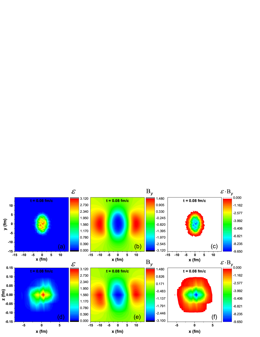
Figure 1: The spatial distributions of the energy density [(a) and (c)], the magnetic field $eB_{y}$ [(b) and (d)], and the product of the energy density and $eB_{y}$ [(e) and (f)] in the transverse plane [(a), (b), and (c)] and reaction plane [(d), (e), and (f)] at $t=0.08$ fm/c in Au+Au collisions at 200 GeV and $b=9$ fm.

III.2 Grid-size dependence

The expression in Eq. (2) involves summations over grids, in which we use the field value at the center of each grid as the mean value in that grid. The EM fields produced in heavy-ion collisions are space-time dependent, thus the size of the grid should be small enough to achieve a reasonable precision. On the other hand, the computing time increases dramatically with the decrease of the grid size. So we have to find an appropriate grid size to balance these two contradictory constraints. In this subsection, we study the grid-size dependence of $\left\langle eB_{y}\right\rangle_{E}$ in order to find an optimized value for the grid size.

We consider Au+Au collisions at 200 GeV and $b=7$ fm. When calculating the average value, we choose the space volume as $-15\text{ fm}<\text{$x$, $y$}<15\text{ fm}$ and $-10\text{ fm}<z<10\text{ fm}$, and divide it into grids with the grid size $dx$, $dy$, and $dz$. Figure 2 shows $\left\langle eB_{y}\right\rangle_{E}$ in the unit $m_{\pi}^{2}$ as functions of time with $dx=dy=0.5\text{ fm}$ and various values of $dz$. One can see that there are peaks when $dz=0.5$ fm and $0.1$ fm. This is because the typical length scale of the magnetic field’s variation is smaller than the grid size in the longitudinal direction due to the Lorentz contraction. In this case, the magnetic field at the grid center cannot represent its mean value in the grid. The peaks in magnetic fields arise when spectators, which generate a narrow distribution of the magnetic field in the $z$ direction, are close to centers of some grids. We notice that results become smooth enough for $dz=0.05$ fm (red line) and $dz=0.03$ fm (black line). Therefore, we will choose $dz=0.05$ fm in later calculations, which is small enough to obtain smooth magnetic fields.

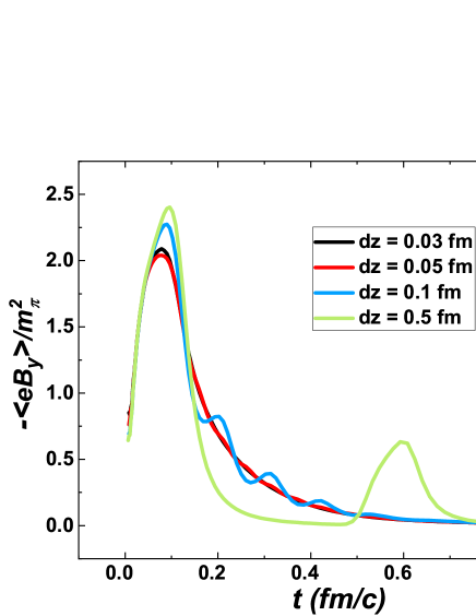
Figure 2: The time dependence of $\left\langle eB_{y}\right\rangle_{E}$ on the longitudinal grid size in Au+Au collisions at 200 GeV and $b=7$ fm.

We also study the dependence of $\left\langle eB_{y}\right\rangle_{E}$ on the grid size in the transverse plane. We fix $dz=0.05$ fm and take $dx=dy=0.05,0.1,0.5$ fm, respectively. We see that the values of $\left\langle eB_{y}\right\rangle_{E}$ are almost independent of $dx$ and $dy$ because the magnetic field slowly varies in the transverse direction. In later calculations we will choose $dx=dy=0.5$ fm.

III.3 Impact parameter and collision energy dependences

The impact parameter dependence of $\left\langle eB_{y}\right\rangle_{E}$ is shown in Fig. 3 for Au+Au collisions at 200 GeV and $b=$1, 4, 7, 8, 9, 10, 11, 12 fm. We see in Fig. 3(a) that all $\left\langle eB_{y}\right\rangle_{E}$ have peak values at about $t=0.08$ fm/c after the collision, and then fastly falls to the values 2 or 3 orders of magnitudes smaller than the peak values in about 1 fm/c. We plot the peak values as functions of the impact parameter in Fig. 3(b). We observe that $\left\langle eB_{y}\right\rangle_{E}$ is proportional to $b$ for small $b$, similar to the behavior of $B_{y}$ at one specific space-time point $(t,\mathbf{x})=(0,0,0,0)$ in Ref. (Deng and Huang, 2012).

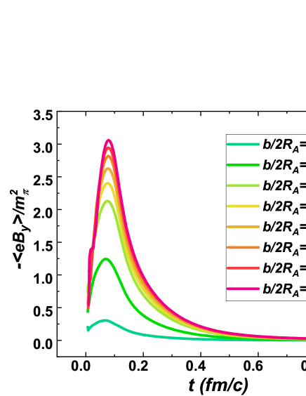
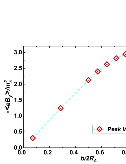
Figure 3: (a): the time evolution of $\left\langle eB_{y}\right\rangle_{E}$ for various impact parameters in Au+Au collisions at 200 GeV. (b): the peak value of $\left\langle eB_{y}\right\rangle_{E}$ as a function of the impact parameter.

The time evolution of $\left\langle eB_{y}\right\rangle_{E}$ at different collision energies and $b=9$ fm is shown in Fig. 4(a). The maximum values of $\left\langle eB_{y}\right\rangle_{E}$ are almost proportional to the collision energy as shown in Fig. 4(b), similar to the behavior of $B_{y}$ at one specific space-time $(t,\mathbf{r})=(0,0,0,0)$ in Ref. (Deng and Huang, 2012). We also observe that $\left\langle eB_{y}\right\rangle_{E}$ reach maximum values earlier at higher than lower collision energies. Meanwhile, $\left\langle eB_{y}\right\rangle_{E}$ decrease slower or live longer at lower collision energies. This is because the magnetic field is mainly generated by spectators moving with the velocity proportional to the collision energy. At very high collision energies, spectators of two nuclei go through each other in such a short time that makes $B_{y}$ behave like a pulse.

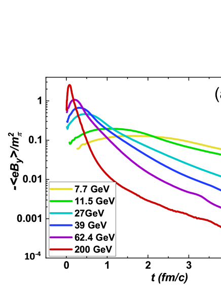
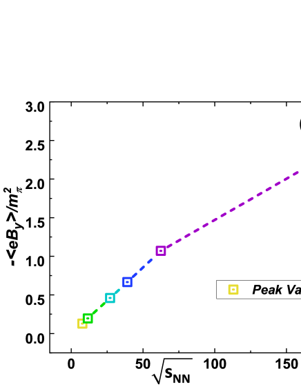
Figure 4: (a): the time evolution of the space-average magnetic field weighted by the energy density, $\left\langle eB_{y}\right\rangle_{E}$, in Au+Au collision at several collision energies and $b=9$ fm. (b): the peak values of $\left\langle eB_{y}\right\rangle_{E}$ as a function of the collision energy.

III.4 Comparison with fields at geometric center

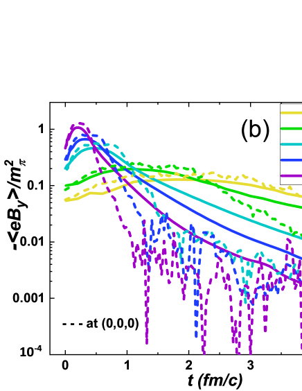
Figure 5: The time evolution of $\left\langle eB_{y}\right\rangle_{E}$ and $eB_{y}$ at the geometric center $\mathbf{r}=(0,0,0)$ at 200 GeV [(a)] and lower energies [(b)] and $b=9$ fm in Au+Au collisions.

In Fig. 5 we make a comparison of $\left\langle eB_{y}\right\rangle_{E}$ with $eB_{y}$ at the space point $\mathbf{r}=(0,0,0)$ or the geometric center as functions of time [denoted as $eB_{y}(t,0,0,0)$] for collisions at 200 GeV [Fig. 5(a)] and lower energies [Fig. 5(b)] and $b=9$ fm. We notice that the peak values of $\left\langle eB_{y}\right\rangle_{E}$ (solid lines) are much smaller, fall much slower or live longer than $eB_{y}(t,0,0,0)$ at all collision energies. This is because the fireball is expanding and regions close to spectators have larger $B_{y}$ than at the geometric center. The much longer lives of $\left\langle eB_{y}\right\rangle_{E}$ than $eB_{y}(t,0,0,0)$ show that it is more appropriate and accurate to use the average field in calculations of any field related effects than the field at a particular space-time point such as the geometric center.

III.5 Comparison between energy and charge density weight

As shown in Eq. (2), one can calculate space-average fields weighted either by the energy or charge density. In Fig. 6, we make a comparison of average fields with two weights in Au+Au collision at 200 GeV and $b=8,9$ fm. We see that the results of $\left\langle eB_{y}\right\rangle_{E}$ (solid lines) are smoother than those of $\left\langle eB_{y}\right\rangle_{C}$ (dashed lines). If we take averages over sufficiently large number of events, fluctuations in average fields weighted by the charge density are expected to be suppressed.

Figure 6: Comparison of $\left\langle eB_{y}\right\rangle_{E}$ (solid lines) and $\left\langle eB_{y}\right\rangle_{C}$ (dashed lines) as functions of time in Au+Au collisions at 200 GeV and $b=8,9$ fm.

IV Squared fields

In this section we calculate the space averages of squared electric and magnetic fields in Au+Au collisions at energies ranging from 7.7 GeV to 200 GeV and $b=9\text{ fm}$ in the central rapidity region. The averages of squared electric and magnetic fields play important roles in the spin alignment of vector mesons (Liang and Wang, 2005; Sheng et al., 2020a, b). The results for $\left\langle(eB_{i})^{2}\right\rangle{}_{E}$ with $i=x,y,z$ are shown in Fig. 7 and those for $\left\langle(eE_{i})^{2}\right\rangle{}_{E}$ are shown in Fig. 8. We see in Fig. 7 that at the same collision energy, the peak value of $\left\langle(eB_{y})^{2}\right\rangle{}_{E}$ is about one order of magnitude larger than that of $\left\langle(eB_{x})^{2}\right\rangle{}_{E}$ and about two (lower energies) to four (higher energies) orders of magnitude larger than that of $\left\langle(eB_{z})^{2}\right\rangle{}_{E}$. For electric fields, as shown in Fig. 8, at the same collision energy, the peak value of $\left\langle(eE_{x})^{2}\right\rangle{}_{E}$ is in the same order of magnitude as that of $\left\langle(eE_{y})^{2}\right\rangle{}_{E}$, both are about one (lower energies) to three (higher energies) orders of magnitude larger than that of $\left\langle(eE_{z})^{2}\right\rangle{}_{E}$.

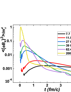
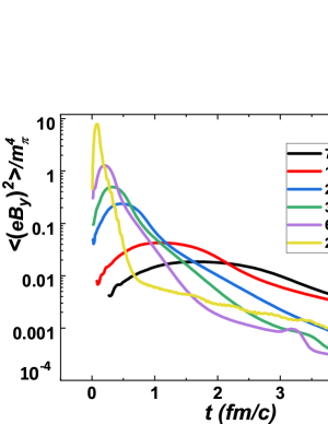
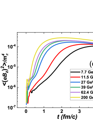
Figure 7: The time evolution of $\left\langle(eB_{i})^{2}\right\rangle{}_{E}$ with $i=x,y,z$ at collision energies ranging from 7.7 GeV to 200 GeV in Au+Au collisions and $b=9$ fm.

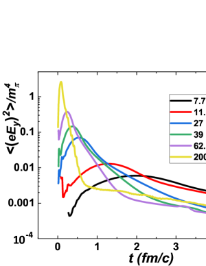
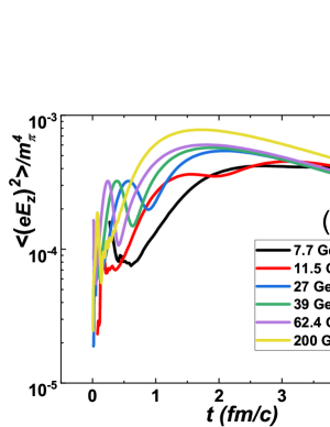
Figure 8: The time evolution of $\left\langle(eE_{i})^{2}\right\rangle{}_{E}$ with $i=x,y,z$ at collision energies ranging from 7.7 GeV to 200 GeV in Au+Au collisions and $b=9$ fm.

The results of the impact parameter dependence of $\left\langle(eB_{i})^{2}\right\rangle_{E}$ and $\left\langle(eE_{i})^{2}\right\rangle_{E}$ are given in Figs. 9 and 10 respectively. The collision energy is set to 200 GeV and the impact parameter is set to $b=1,2,4,6,7,10,12$ fm. We see in Figs. 9(a) and (b) that $\left\langle(eB_{x})^{2}\right\rangle_{E}$ and $\left\langle(eB_{y})^{2}\right\rangle_{E}$ reach their maximum values at about $t=0.08$ fm/c and fall fastly towards zero after $t=1$ fm/c. We observe that $\left\langle(eB_{y})^{2}\right\rangle_{E}$ increases with the impact parameter, similar to $\left\langle eB_{y}\right\rangle_{E}$ . However, the peak values of$\left\langle(eB_{x})^{2}\right\rangle_{E}$ reach a maximum at an intermediate impact parameter. Such a non-monotonous behaviour in the maximum values of $\left\langle(eB_{x})^{2}\right\rangle_{E}$ reflects charge fluctuations in the fireball. For small impact parameters, fluctuations are relatively small comparing with large average charge densities in the collision zone. For large impact parameters, fluctuations are suppressed because of low energy densities in the collision zone. The values of $\left\langle(eB_{z})^{2}\right\rangle_{E}$, as shown in Fig. 9(c), are about three and four orders of magnitude smaller than $\left\langle(eB_{x})^{2}\right\rangle_{E}$ and $\left\langle(eB_{y})^{2}\right\rangle_{E}$ respectively, because the $z$-component of the magnetic field is suppressed by the Lorentz factor for particles moving in the $z$-direction. We also see the peak values of $\left\langle(eB_{z})^{2}\right\rangle_{E}$ reach a maximum at an intermediate impact parameter.

Similar impact parameter dependences also exist for squared electric fields, $\left\langle(eE_{i})^{2}\right\rangle_{E}$, as shown in Fig. 10. The maximum value of $\left\langle(eE_{x})^{2}\right\rangle_{E}$ appears at $b=2$ fm, while the maximum values of $\left\langle(eE_{y})^{2}\right\rangle_{E}$ and $\left\langle(eE_{z})^{2}\right\rangle_{E}$ appear at $b=4$ fm. The magnitudes of $\left\langle(eE_{x})^{2}\right\rangle_{E}$ and $\left\langle(eE_{y})^{2}\right\rangle_{E}$ are comparable, which are about three orders of magnitude larger than $\left\langle(eE_{z})^{2}\right\rangle_{E}$. For the impact parameter $b\geq 7$ fm, there are two peaks in $\left\langle(eE_{x})^{2}\right\rangle_{E}$ as functions of time. This is because $E_{x}$ generated by the fireball and spectators cancel in some space-time region. For small impact parameters, $E_{x}$ generated by the fireball is significantly larger than that by spectators, thus the second peak disappears.

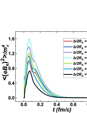
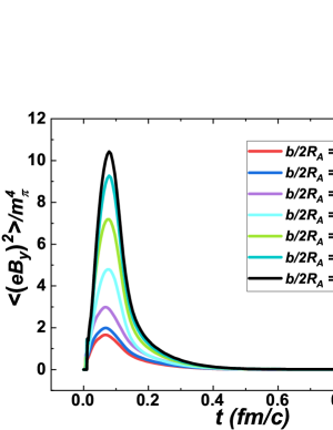
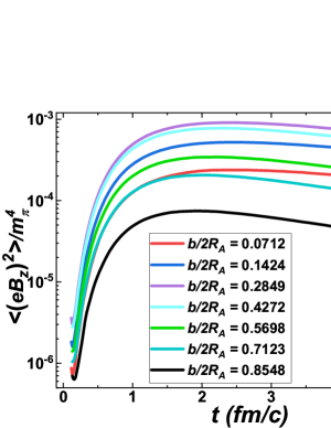
Figure 9: Time evolution of $\left\langle(eB_{i})^{2}\right\rangle_{E}$ with $i=x,y,z$ for various impact parameters in Au+Au collisions at $200$ GeV.

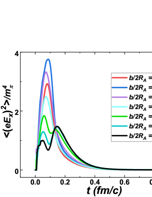
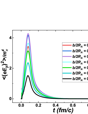
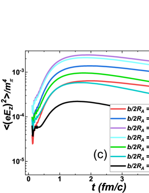
Figure 10: Time evolution of $\left\langle(eE_{i})^{2}\right\rangle_{E}$ with $i=x,y,z$ for various impact parameters in Au+Au collisions at $200$ GeV.

V EM anomaly

In this section we study the EM anomaly $e^{2}\mathbf{E}\cdot\mathbf{B}$ in heavy ion collisions. The spatial distribution of $e^{2}\mathbf{E}\cdot\mathbf{B}$ at $t=0.08$ fm/c for Au+Au collisions at 200 GeV and $b=9$ fm is shown in Fig. 11. We choose $t=0.08$ fm/c because the magnetic field reaches its maximum value at this time as shown in Fig. 3. The anomaly $e^{2}\mathbf{E}\cdot\mathbf{B}$ is symmetric for flipping the sign of $x$ and anti-symmetric for flipping the sign of $y$, i.e. it is a dipolar distribution. Figure 11 (b) shows the spatial distribution of $e^{2}\mathbf{E}\cdot\mathbf{B}$ times the energy density, which also has a dipolar structure. When directly calculating the space-average of the EM anomaly weighted by the energy density, it is natural to see $\left\langle e^{2}\mathbf{E}\cdot\mathbf{B}\right\rangle_{E}=0$, but the averages in upper ($+y$) and lower ($-y$) half space are all nonzero. In Fig. 12, we show $\left\langle e^{2}\mathbf{E}\cdot\mathbf{B}\right\rangle_{E}$ as functions of time in the $-y$ region at 200 GeV [Fig. 12(a)] and lower energies 62.4, 39, 27, 11.5, 7.7 GeV [Fig. 12(b)], and a comparison has been made between $\left\langle e^{2}\mathbf{E}\cdot\mathbf{B}\right\rangle_{E}$ and $e^{2}\mathbf{E}\cdot\mathbf{B}$ at the space point $(0,-4,0)$ fm at each energy. Comparing with $e^{2}\mathbf{E}\cdot\mathbf{B}$ at the space point $(0,-4,0)$ fm, $\left\langle e^{2}\mathbf{E}\cdot\mathbf{B}\right\rangle_{E}$ have smaller peak values and decrease slower in time.

In Fig. 13, we give peak values of $\left\langle e^{2}\mathbf{E}\cdot\mathbf{B}\right\rangle_{E}$ as a function of the number of participants at 200 GeV, compared with the slope parameter for the difference in charge-dependent elliptic flows for charged pions, which is measured by the STAR collaboration (Adamczyk et al., 2015). We confirm that the $N_{\text{part}}$ dependence of $\left\langle e^{2}\mathbf{E}\cdot\mathbf{B}\right\rangle_{E}$ is consistent with that of the slope parameter. We note that $\left\langle e^{2}\mathbf{E}\cdot\mathbf{B}\right\rangle_{E}$ in the $+y$ and $-y$ region have an opposite sign, leading to opposite chiral charges in the $\pm y$ regions and therefore a charge separation with respect to the reaction plane because of the CME. Similar to the CMW, this mechanism can also induce the charge-dependence $v_{2}$ observed in the STAR experiments (Adamczyk et al., 2015; Zhao et al., 2019a). Our results of $\left\langle e^{2}\mathbf{E}\cdot\mathbf{B}\right\rangle_{E}$ is about 50% smaller than the values in Ref. (Zhao et al., 2019a) because different methods are used when calculating zone-averages.

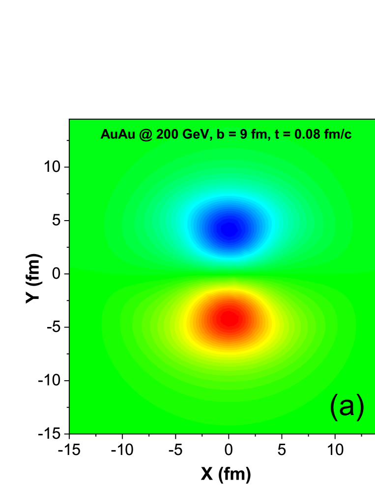
Figure 11: The spatial distributions of $e^{2}\mathbf{E}\cdot\mathbf{B}$ [(a)] and the product of the energy density and $e^{2}\mathbf{E}\cdot\mathbf{B}$ [(b)].

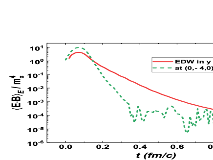
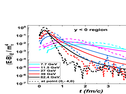
Figure 12: The time evolution of the space-average EM anomaly weighted by the energy density $\left\langle e^{2}\mathbf{E}\cdot\mathbf{B}\right\rangle_{E}$ in the $-y$ region in Au+Au collision at 200 GeV [(a)] and lower energies [(b)] and $b=9$ fm. The value of $e^{2}\mathbf{E}\cdot\mathbf{B}$ at the space point $(0,-4,0)$ fm as a function of time is also shown for a comparison.

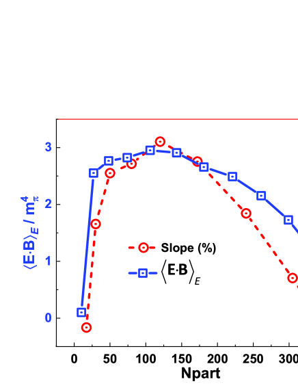
Figure 13: The peak values of $\left\langle e^{2}\mathbf{E}\cdot\mathbf{B}\right\rangle_{E}$ and the slope parameter as functions of the number of participants $N_{\text{part}}$ in Au+Au collisions at 200 GeV.

VI Parameterization for space-average fields

In previous sections we have presented results of space-average fields for various collision energies and impact parameters. In this section, we give parameterized formula for $\left\langle eB_{y}\right\rangle_{E}$, $\left\langle(eB_{i})^{2}\right\rangle_{E}$, $\left\langle(eE_{i})^{2}\right\rangle_{E}$, for $i=x,y$, and $\left\langle e^{2}{\bf E}\cdot{\bf B}\right\rangle_{E}$, as functions of time. The other components $\left\langle eB_{x,z}\right\rangle_{E}$, $\left\langle eE_{x,y,z}\right\rangle_{E}$, $\left\langle(eB_{z})^{2}\right\rangle_{E}$ and $\left\langle(eE_{z})^{2}\right\rangle_{E}$ are too small to be parameterized. These analytical formulas are useful in studies of field-related effects in heavy-ion collisions.

We notice from Fig. 3 and Fig. 4 that $\left\langle eB_{y}\right\rangle_{E}$ as a function of time always has one peak at a specific time and the peak value depends on both the impact parameter and the collision energy, as shown in Figs. 3(b) and Fig. 4(b). The average quantities $\left\langle(eB_{x})^{2}\right\rangle_{E}$, $\left\langle(eB_{y})^{2}\right\rangle_{E}$, $\left\langle(eE_{y})^{2}\right\rangle_{E}$, and $\left\langle e^{2}\mathbf{E}\cdot\mathbf{B}\right\rangle_{E}$ in Fig. 7, Fig. 8, and Fig. 12 also have the one-peak structure similar to $\left\langle eB_{y}\right\rangle_{E}$. For the time behaviors of these quantities, we assume the following parameterization

$$\left\langle F\right\rangle_{E}(t)=M_{F}f\left[(\gamma t-t_{F})/(\text{fm/c})\right],$$ (5)

where $F$ represents $eB_{y}$, $(eB_{x})^{2}$, $(eB_{y})^{2}$, $(eE_{y})^{2}$ or $e^{2}\mathbf{E}\cdot\mathbf{B}$, $M_{F}$ denotes the maximum value of $\left\langle F\right\rangle_{E}$ with $t_{F}$ being its corresponding time multiplied by the Lorentz factor $\gamma=\sqrt{s_{NN}}/(2m_{p})$ with the proton mass $m_{p}$, and $f(x)$ is a function of dimensionless variable $x$ and has the maximum value $1$ at $x=0$. We can further parameterize $M_{F}$ and $t_{F}$ in second polynomials of $\gamma$ and the dimensionless impact parameter $\overline{b}=b/(2R_{A})$ with $R_{A}$ being the nuclear radius and $R_{A}=7.02$ fm for gold nuclei,

$$M_{F} = \alpha_{M}(1+c_{M}^{(1)}\gamma+c_{M}^{(2)}\gamma^{2})(1+c_{M}^{(3)}\overline{b}+c_{M}^{(4)}\overline{b}^{2}),$$ (6)

$$t_{F} = \alpha_{t}(1+c_{t}^{(1)}\gamma+c_{t}^{(2)}\gamma^{2})(1+c_{t}^{(3)}\overline{b}+c_{t}^{(4)}\overline{b}^{2}),$$ (7)

where the parameters $\alpha_{M}$, $c_{M}^{(i)}$, $\alpha_{t}$, and $c_{t}^{(i)}$, $i=1,2,3,4$ are determined by fitting the peak values of $\left\langle F\right\rangle_{E}(t)$. They vary for different quantities of $F$, as shown in Table 1 and Table 2. Note that $\left\langle F\right\rangle_{E}$ reaches its maximum value at $t\simeq t_{F}/\gamma$ instead of $t=0$ at high energies, which is attributed to the finite size of the colliding nuclei. We see in Table 1 that the peak value of $\left\langle eB_{y}\right\rangle_{E}$ is proportional to $\gamma b$ at the leading order, similar to the behavior found in Ref. (Deng and Huang, 2012) about the magnetic field at a specific space-time point. The deviation from the linear behavior is described by second power terms of $\gamma$ and $b$. However, the peak values of squared fields $\left\langle eB_{x,y}^{2}\right\rangle_{E}$ and $\left\langle eE_{y}^{2}\right\rangle_{E}$ do not linearly depend on $b$ at the leading order, this is because the average squared fields are mainly dominated by fluctuations. We also see that the peak value of $\left\langle e^{2}\mathbf{E}\cdot\mathbf{B}\right\rangle_{E}$ is linearly proportional to $b$ at the leading order, same as $\left\langle eB_{y}\right\rangle_{E}$.

$F$	$\alpha_{M}$	$c_{M}^{(1)}$	$c_{M}^{(2)}$	$c_{M}^{(3)}$	$c_{M}^{(4)}$
$eB_{y}$	$6.266\times 10^{-4}\,Z\gamma\bar{b}m_{\pi}^{2}$	$2.123\times 10^{-3}$	$-3.855\times 10^{-5}$	$0.3890$	$-0.6430$
$(eB_{x})^{2}$	$1.053\times 10^{-8}\,Z^{2}\gamma^{2}m_{\pi}^{4}$	$7.624\times 10^{-4}$	$-3.965\times 10^{-6}$	$4.018$	$-4.954$
$(eB_{y})^{2}$	$1.446\times 10^{-8}\,Z^{2}\gamma^{2}m_{\pi}^{4}$	$4.135\times 10^{-3}$	$-7.086\times 10^{-5}$	$12.97$	$6.791$
$(eE_{y})^{2}$	$5.592\times 10^{-8}\,Z^{2}\gamma^{2}m_{\pi}^{4}$	$-4.260\times 10^{-4}$	$-1.807\times 10^{-5}$	$2.089$	$-3.278$
$e^{2}{\bf E}\cdot{\bf B}$	$1.399\times 10^{-7}\,Z^{2}\gamma^{2}\bar{b}m_{\pi}^{4}$	$2.033\times 10^{-3}$	$-5.523\times 10^{-5}$	$0.4472$	$-1.213$

Table 1: The parameters in $M_{F}$ for various quantities of $F$. Here $Z$ is the proton number of the colliding nuclei with $Z=79$ for Au+Au collisions.

$F$	$\alpha_{t}$	$c_{t}^{(1)}$	$c_{t}^{(2)}$	$c_{t}^{(3)}$	$c_{t}^{(4)}$
$eB_{y}$	$5.681$	$-1.368\times 10^{-3}$	$3.254\times 10^{-5}$	$0.3569$	$-0.1061$
$(eB_{x})^{2}$	$7.239$	$-3.820\times 10^{-3}$	$2.461\times 10^{-5}$	$-0.1821$	$0.4701$
$(eB_{y})^{2}$	$5.186$	$-1.840\times 10^{-3}$	$3.726\times 10^{-5}$	$0.8977$	$-0.5478$
$(eE_{y})^{2}$	$8.043$	$-1.930\times 10^{-3}$	$2.368\times 10^{-5}$	$0.06777$	$0.09616$
$e^{2}{\bf E}\cdot{\bf B}$	$6.571$	$-1.173\times 10^{-3}$	$2.738\times 10^{-5}$	$0.4465$	$-0.3172$

Table 2: The parameters in $t_{F}$ for various quantities of $F$.

The function $f(x)$ in Eq. (5) can be further written as a two-component form

$$f(x)=f_{a}(x)+f_{b}(x),$$ (8)

where $f_{a}(x)$ and $f_{b}(x)$ describe the early and later stage of the evolution, respectively. We thus determine $f_{a}(x)$ by fitting numerical results before the peak time and then determine $f_{b}(x)$ by fitting the difference between numerical results and $f_{a}(x)$. The parameterization reads

$$f_{a}(x) = \left[1+c_{a}^{(1)}(x^{2})^{c_{a}^{(2)}}\right]^{-1},$$

$$f_{b}(x) = \theta(x-c_{b}^{(1)})\exp\left[c_{b}^{(2)}-c_{b}^{(3)}(x-c_{b}^{(1)})^{c_{b}^{(4)}}\right](x-c_{b}^{(1)})^{c_{P}^{(5)}},$$ (9)

where $\theta(x)$ is the step function with $\theta(x>0)=1$ and $\theta(x<0)=0$. The values of the parameters $c_{a}^{(i)}$ and $c_{b}^{(j)}$ with $i=1,2$ and $j=1,2,3,4,5$ are given in Table 3 which are determined by fitting the numerical results of Au+Au collisions at $200$ GeV and $b=9$ fm. In Fig. 14, we plot $f_{a}$, $f_{b}$, and $f=f_{a}+f_{b}$ for $\left\langle eB_{y}\right\rangle_{E}$. For comparison, we also show the numerical results for $\left\langle eB_{y}\right\rangle_{E}$ (black dots) from the UrQMD calculation. We see that $f_{a}$ dominates at the early stage while $f_{b}$ dominates at the later stage as expected.

$F$	$c_{a}^{(1)}$	$c_{a}^{(2)}$	$c_{b}^{(1)}$	$c_{b}^{(2)}$	$c_{b}^{(3)}$	$c_{b}^{(4)}$	$c_{b}^{(5)}$
$eB_{y}$	$3.355\times 10^{-3}$	$1.609$	$3.232$	$11.20$	$14.58$	$0.2267$	$5.217$
$(eB_{x})^{2}$	$7.744\times 10^{-3}$	$1.634$	$2.167$	$1.774$	$4.897$	$0.3830$	$3.921$
$(eB_{y})^{2}$	$2.307\times 10^{-3}$	$1.918$	$2.808$	$6.659$	$17.24$	$-0.9004$	$-2.867$
$(eE_{y})^{2}$	$0.02924$	$1.294$	$2.216$	$-1.791$	$2.163$	$0.4969$	$2.7374$
$e^{2}{\bf E}\cdot{\bf B}$	$7.744\times 10^{-3}$	$1.634$	$4.046$	$17.08$	$20.29$	$0.2147$	$5.842$

Table 3: The parameters in $f(x)$ for various kinds of $F$.

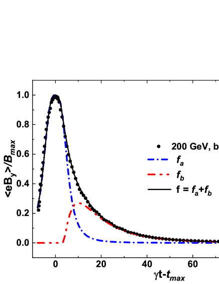
Figure 14: The function $f(x)$ for $\left\langle eB_{y}\right\rangle_{E}$ in Au+Au collisions at 200 GeV and $b=9$ in Eqs. (8, 9).

The special quantity is $\left\langle(eE_{x})^{2}\right\rangle_{E}$, which has two peaks as shown in Fig. 8, different from $\left\langle eB_{y}\right\rangle_{E}$, $\left\langle(eB_{x,y})^{2}\right\rangle_{E}$, $\left\langle(eE_{y})^{2}\right\rangle_{E}$, and $\left\langle e^{2}\mathbf{E}\cdot\mathbf{B}\right\rangle_{E}$. We therefore parameterize $\left\langle(eE_{x})^{2}\right\rangle_{E}$ as

$$\left\langle(eE_{x})^{2}\right\rangle=M_{1}f_{a}\left[(\gamma t-t_{1})/(\text{fm/c})\right]+M_{2}f_{b}\left[(\gamma t-t_{2})/(\text{fm/c})\right]$$ (10)

where $M_{1}$ and $t_{1}$ are for the first peak, while $M_{2}$ and $t_{2}$ are for the second peak. We assume the same parameterization, Eqs. (6) and (7), for $M_{1,2}$ and $t_{1,2}$ as functions of $\gamma$ and $\overline{b}$. By fitting numerical results, the parameters are obtained and given in Table 4 and Table 5. Meanwhile, $f_{a}$ and $f_{b}$ are also parameterized by Eq. (9). Again, the parameters in $f_{a}$ and $f_{b}$ are fixed by fitting $\left\langle(eE_{x})^{2}\right\rangle_{E}$ for Au+Au collisions at 200 GeV and $b=9$ fm, the results are given in Table 6.

It is worthwhile to mention that the parameters in $f$ in Eq. (9) can be determined by fitting numerical results at any collision energy and any impact parameter with little difference although they are determined in this paper by fitting numerical results at $200$ GeV and $b=9$ fm. This means that $f$ is almost universal in a wide range of collision energies from $7.7$ GeV to $200$ GeV and impact parameters from $0$ to $2R_{A}$.

	$\alpha_{M}$	$c_{M}^{(1)}$	$c_{M}^{(2)}$	$c_{M}^{(3)}$	$c_{M}^{(4)}$
$M_{1}$	$5.183\times 10^{-8}\,Z^{2}\gamma^{2}m_{\pi}^{4}$	$-3.054\times 10^{-4}$	$-9.345\times 10^{-6}$	$-0.8886$	$0.05202$
$M_{2}$	$-5.908\times 10^{-9}\,Z^{2}\gamma^{2}m_{\pi}^{4}$	$1.153\times 10^{-3}$	$-2.619\times 10^{-5}$	$-14.17$	$9.395$

Table 4: The parameters in $M_{1}$ and $M_{2}$ for $\left\langle(eE_{x})^{2}\right\rangle$.

	$\alpha_{t}$	$c_{t}^{(1)}$	$c_{t}^{(2)}$	$c_{t}^{(3)}$	$c_{t}^{(4)}$
$t_{1}$	$9.260$	$-3.251\times 10^{-3}$	$2.653\times 10^{-5}$	$-0.4211$	$-0.1054$
$t_{2}$	$6.935$	$-2.135\times 10^{-3}$	$2.529\times 10^{-5}$	$3.238$	$-2.170$

Table 5: The parameters in $t_{1}$ and $t_{2}$ for $\left\langle(eE_{x})^{2}\right\rangle$.

	$c_{a}^{(1)}$	$c_{a}^{(2)}$	$c_{b}^{(1)}$	$c_{b}^{(2)}$	$c_{b}^{(3)}$	$c_{b}^{(4)}$	$c_{b}^{(5)}$
$\left\langle(eE_{x})^{2}\right\rangle_{E}$	$0.02856$	$1.356$	$-15.81$	$16.73$	$235.6$	$-1.547$	$-4.926$

Table 6: The parameters in $f_{a}$ and $f_{b}$ for $\left\langle(eE_{x})^{2}\right\rangle$.

VII Summary and conclusions

In this paper we use the UrQMD model to simulate the electromagnetic fields in heavy ion collisions. In order to quantify the effects on the hot and dense matter from electromagnetic fields, we propose the space-average quantities (fields, squared fields, scalar product of the electric and magnetic field, etc.) weighted by the energy or charge density as functions of time to be barometers for field-related effects. It is found that the average magnetic field increases with time and reaches its maximum value soon after the collision, then it quickly damps to zero. It is found that the peak value of the average magnetic field is proportional to the collision energy and the impact parameter. Comparing with the magnetic field at the geometric center of the collision, the average quantities has a little smaller peak value shortly after the collision but damps much slower or live much longer at the later stage.

By fitting numerical results of electromagnetic fields with the UrQMD model, we use analytical formula to parameterize the space-average quantities, fields, squared fields, and electromagnetic anomaly (scalar product of the electric and magnetic field), as functions of time. The parameterization formulas are expressed in terms of the Lorentz factor encoding the collision energy and the relative impact parameter $\overline{b}=b/(2R_{A})$. We have checked that the parameterization formulas are in good agreement with numerical results for collisions at energies from 7.7 GeV to 200 GeV and impact parameters from 0 to $12$ fm.

In the calculation of this paper, we do not introduce the electric conductivity which is expected to slow down the damping of electromagnetic fields and deserves a detailed study in the future.