DoT: An efficient Double Transformer for NLP tasks with tables

Abstract

Transformer-based approaches have been successfully used to obtain state-of-the-art accuracy on natural language processing (NLP) tasks with semi-structured tables. These model architectures are typically deep, resulting in slow training and inference, especially for long inputs. To improve efficiency while maintaining a high accuracy, we propose a new architecture, $DoT$, a double transformer model, that decomposes the problem into two sub-tasks: A shallow pruning transformer that selects the top-$K$ tokens, followed by a deep task-specific transformer that takes as input those K tokens. Additionally, we modify the task-specific attention to incorporate the pruning scores. The two transformers are jointly trained by optimizing the task-specific loss. We run experiments on three benchmarks, including entailment and question-answering. We show that for a small drop of accuracy, $DoT$ improves training and inference time by at least 50%. We also show that the pruning transformer effectively selects relevant tokens enabling the end-to-end model to maintain similar accuracy as slower baseline models. Finally, we analyse the pruning and give some insight into its impact on the task model.

1 Introduction

Recently, transfer learning with large-scale pre-trained language models has been successfully used to solve many NLP tasks Devlin et al. (2019); Radford et al. (2019); Liu et al. (2019). In particular, transformer models have been used to solve tasks that include semi-structured table knowledge, such as table question answering Herzig et al. (2020) and entailment Wenhu et al. (2019); Eisenschlos et al. (2020) – a binary classification task to support or refute a sentence based on the table’s content.

While transformer models lead to significant improvements in accuracy, they suffer from high computation and memory cost, especially for large inputs. The total computational complexity per layer for self-attention is $O(n^{2}d)$ Vaswani et al. (2017), where $n$ is the input sequence length, and $d$ is the embedding dimension. Using longer sequence lengths translates into increased training and inference time.

Improving the computational efficiency of transformer models has recently become an active research topic. To the best of our knowledge, the only technique that was applied to nlp tasks with semi-structured tables is heuristic pruning. Eisenschlos et al. (2020) show on the TabFact data set Wenhu et al. (2019) that using heuristic pruning accelerates the training time while achieving a similar accuracy. This raises the question of whether a better pruning strategy can be learned.

We propose to use $DoT$, a double transformer model (Figure 1): A first transformer – which we call pruning transformer – selects $k$ tokens given a query and a table and a task-specific transformer solves the task based on these tokens. Decomposing the problem into two simpler tasks imposes additional structure that makes training more efficient: The first model is shallow, allowing the use of long input sequences at moderate cost, and the second model is deeper and uses the shortened input that solves the task. The combined model achieves a better efficiency-accuracy trade-off.

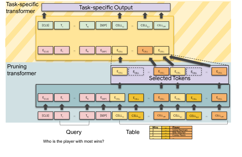
Figure 1: Pruning with a double transformer $DoT$. The pruning model selects the $k$ most relevant tokens and passes them to the task model. The pruning model is small, allowing the use of long input sequences.

The pruning transformer is based on the TAPAS QA model Herzig et al. (2020). TAPAS answers questions by selecting tokens from a given table. This problem is quite similar to the pruning task. The second transformer is a task-specific model adapted for each task to solve: We use another TAPAS QA model for QA and a classification model  Eisenschlos et al. (2020) for entailment. In Section 2, we explain how we jointly learn both models by incorporating the pruning scores into the attention mechanism.

$DoT$ achieves a better trade-off between efficiency and accuracy on three datasets. We show that the pruning transformer selects relevant tokens, resulting in higher accuracy for longer input sequences. We study the meaning of relevant tokens and show that the selection is deeply linked to solving the main task by studying the answer token scores. We open source the code in http://github.com/google-research/tapas.

2 The $DoT$ Model

As show in Figure 1, the double transformer $DoT$ is composed of two transformers: the pruning transformer selects the most relevant $k$ tokens followed by a task-specific model that operates on the selected tokens to solve the task. The two transformers are learned jointly. $DoT$ loss is detailed in Appendix A.2. We explore learning the pruning model using an additional loss in Appendix C.2.

Let $q$ be the query (or statement) and $T$ the table. The transformer takes as input the embedding $E=[E_{[CLS]};E_{q};E_{[SEP]};E_{T}]$, composed of the query and table embeddings. The pruning transformer computes the probability $P(t|q,T)$ of the token $t$ being relevant to solve the example. We derive the pruning score $s_{t}=\log(P(t|q,T))$ and keep the top-$k$ tokens. The pruning scores are then passed to the task transformer as shown in Figure 2.

To enable the joint learning, we change the attention scores of the task model. For a normal transformer Vaswani et al. (2017), given the input embedding $E_{t}$ at position $t$, for each layer and attention head, the self-attention output is given by a linear combination of the value vector projections using the attention matrix.

Each row of the attention matrix is obtained by a softmax on the attention scores $z^{<t,t^{\prime}>}$ given by

where $W_{Q}$ and $W_{K}$ represent the query and key projections for that layer and head. In our task model we add a negative bias term and replace this equation with

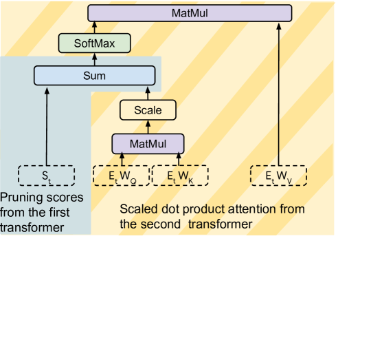
Figure 2: Scaled dot product attention of the task model. We change the attention architecture Vaswani et al. (2017) – the dashed bloc – by adding the pruning scores – the solid bloc. The pruning scores affect the task model’s attention in all layers. This enables back propagation for both models based on a single loss.

Thus, the attention scores provide a notion of token relevance – detailed in Appendix A.1 – and enable end-to-end learning of both models, letting $DoT$ define the top-$K$ tokens.

Unlike previous soft-masking methods Bastings et al. (2019); De Cao et al. (2020), ours coincides exactly with removing the input token $t$ when $P(t|q,T)\to 0$. We prove this formally in Appendix A.3.

We explore two different pruning strategies: token selection defined as discussed above and column selection where we average all token scores in each column.

3 Experimental Setup

We compare our approach against models using heuristic pruning.
Cell concatenation ($CC$) The TAPAS model uses a default heuristic to limit the input tokens. The objective of the algorithm is to fit an equal number of tokens for each cell. This is done by first selecting the first token from each cell, then the second and so on until the desired limit is reached.
Heuristic exact match ($HEM$) Eisenschlos et al. (2020). This method scores the columns based on their similarity to the question, where similarity is defined by token overlap.

We introduce a notation to clarify the setup: $DoT(1^{st}_{type}\xrightarrow[]{top\mbox{-}k}2^{nd}_{type})$. The $type$ correspond to the model size: small ($s$), medium ($m$) or large ($l$) as defined in Turc et al. (2019). For example, $CC\xrightarrow[]{1024}DoT(s\xrightarrow[]{256}l)$ denotes a $CC$ pre-processing to select $1024$ tokens passed to the $DoT$ model: one small pruning model that selects $256$ tokens and feeds them into a large task model.

Baselines and $DoT$ (hyper-parameters in Appendix B.1) are initialized from models pre-trained with a MASK-LM task, the intermediate pre-training data Eisenschlos et al. (2020) and following Herzig et al. (2020) on SQA Iyyer et al. (2017). The $DoT$ transformers’ complexity – detailed in Appendix B.3 – is similar to a normal transformer where only some constants are changed.

We evaluate $DoT$ on three datasets.
WIKISQL  Zhong et al. (2017) is a corpus of $80,654$ questions with SQL queries, related to $24,241$ Wikipedia tables. Here we train and test in the weakly-supervised setting where the answer to the question is the result of the SQL applied to the table. The metric we use is denotation accuracy.
WIKITQ  Pasupat and Liang (2015) consists of $22,033$ question-answer pairs on $2,108$ Wikipedia tables. The questions are complex and often require comparisons, superlatives or aggregation. The metric we use is the denotation accuracy as computed by the official evaluation script.
TabFact  Wenhu et al. (2019) contains $118$K statements about $16$K Wikipedia tables, labeled as either entailed or refuted. The dataset requires both linguistic reasoning and symbolic reasoning with operations such as comparison, filtering or counting. We use the classification accuracy as metric.

In all our experiments we report results for $DoT$ using token selection for WIKISQL and TabFact and a column selection for WIKITQ.

4 Results

Dataset	WIKISQL			TabFact			WIKITQ
Model	test accuracy	Best	NPE/s	test accuracy	Best	NPE/s	test accuracy	Best	NPE/s
state-of-the-art	$83.9$			$81.0$			$51.8\pm 0.6$	$52.3$
$\text{\ \ \ \ }CC\text{ }\xrightarrow[]{256}\textsc{TAPAS}(l)$	$76.4\pm 0.3$	$77.15$	$1870$	$75.1\pm 0.3$	$76.13$	$1900$	$44.8\pm 0.5$	$45.47$	$1900$
$\text{\ \ \ \ }CC\text{ }\xrightarrow[]{512}\textsc{TAPAS}(l)$	$83.6\pm 0.1$	$83.65$	$800$	$81.3\pm 0.2$	$81.60$	$870$	$52.2\pm 0.5$	$52.74$	$810$
$\text{\ \ \ \ }CC\xrightarrow[]{1024}\textsc{TAPAS}(l)$	$86.0\pm 0.3$	$86.6$	$270$	$81.6\pm 0.1$	$81.64$	$300$	$53.9\pm 0.2$	$54.30$	$270$
$\text{\ \ \ \ }CC\xrightarrow[]{1024}DoT(s\text{ }\xrightarrow[]{256}l)$	$74.2\pm 3.6$	$84.27$	$1250$	$81.0\pm 0.1$	$81.17$	$1300$	$48.1\pm 2.4$	$49.47$	$1250$
$\text{\ \ \ \ }CC\xrightarrow[]{1024}DoT(m\xrightarrow[]{256}l)$	$83.6\pm 0.5$	$84.67$	$950$	$79.0\pm 0.5$	$81.28$	$930$	$50.1\pm 0.5$	$50.14$	$950$
$HEM\xrightarrow[]{256}\textsc{TAPAS}(l)$	$77.4\pm 0.3$	$77.97$	$1870$	$75.5\pm 0.2$	$75.80$	$1900$	$47.3\pm 0.1$	$47.70$	$1900$
$HEM\text{ }\xrightarrow[]{512}\textsc{TAPAS}(l)$	$83.8\pm 0.4$	$84.75$	$800$	$82.0\pm 0.3$	$82.07$	$870$	$52.7\pm 0.4$	$53.61$	$810$
$HEM\xrightarrow[]{1024}\textsc{TAPAS}(l)$	$85.9\pm 0.0$	$85.94$	$270$	$80.6\pm 0.0$	$80.6$	$300$	$54.0\pm 0.9$	$54.93$	$270$
$HEM\xrightarrow[]{1024}DoT(s\text{ }\xrightarrow[]{256}l)$	$85.3\pm 0.4$	$85.76$	$1250$	$81.6\pm 0.3$	$81.74$	$1300$	$40.9\pm 0.2$	$41.23$	$1250$
$HEM\xrightarrow[]{1024}DoT(m\xrightarrow[]{256}l)$	$85.5\pm 0.2$	$85.82$	$950$	$81.8\pm 0.0$	$81.94$	$930$	$40.1\pm 2.4$	$49.13$	$950$

Table 1: Efficiency accuracy trade-off. We run $DoT$ with token pruning for WIKISQL and TabFact and column pruning for WIKITQ. The state-of-the-art (detailed in Appendix B.2) corresponds to the models of Min et al. (2019) for WIKISQL, Eisenschlos et al. (2020) for TabFact and Yin et al. (2020) for WIKITQ. For each dataset, the state-of-the-art, the best baseline model on accuracy, and the $DoT$ models that reach the best accuracy efficiency trade-off are highlighted.

The baseline TAPAS model outperforms the previous state-of-the-art on all datasets (Table 1): $+2.1$ for WIKISQL ($CC\xrightarrow[]{1024}\textsc{TAPAS}(l)$), $+1.07$ for TabFact ($HEM\xrightarrow[]{512}\textsc{TAPAS}(l)$), and $+1.3$ for WIKITQ ($HEM\xrightarrow[]{1024}\textsc{TAPAS}(l)$).

Efficiency accuracy trade-off

Table 1 reports the accuracy test results along with the average number of processed examples per second $NPE/s$ computed at training time. Using $HEM$ as pre-processing step improves $DoT$ models compared to $CC$ for both WIKISQL and TabFact. $DoT(m)$ and $DoT(s)$ reach better efficiency accuracy trade-off for WIKISQL: with a small drop of accuracy by $0.4\%$ (respectively $0.7\%$), they are $3.5$ (respectively $4.6$) times faster than the best baseline. For TabFact dataset, $DoT$ is compared to a faster baseline than the one used for WIKISQL as it takes only $512$ input tokens instead of $1024$. $DoT(s)$ still achieves a good trade-off: with a decrease of $0.4\%$ of accuracy it is $1.5$ times faster. Unlike the previous datasets, WIKITQ is a harder task to solve and requires passing more data. By restricting $DoT(m)$ to select only $256$ tokens we decrease the accuracy by a bigger drop $3.9\%$ to be $3.5$ times faster compared to $HEM\xrightarrow[]{1024}\textsc{TAPAS}(l)$.

Small task models

The previous results, raise the question of whether a smaller task model can reach a similar accuracy. To answer this question, we compare $\xrightarrow[]{1024}DoT(s\text{ }\xrightarrow[]{256}l)$ to $\xrightarrow[]{1024}\mbox{TAPAS}(s)$ and $\xrightarrow[]{256}\mbox{TAPAS}(l)$ in Table 2. $DoT$ outperforms the smaller models showing the importance of using both transformers.

Dataset	WIKISQL		TabFact		WIKITQ
Model	test accuracy	NPE/s	test accuracy	NPE/s	test accuracy	NPE/s
$CC\xrightarrow[]{1024}DoT(m\xrightarrow[]{256}l)$	$83.6\pm 0.5$	$950$	$79.0\pm 0.9$	$930$	$50.1\pm 0.5$	$950$
$CC\>\>\xrightarrow[]{256}\mbox{TAPAS}(l)$	$76.4\pm 0.3$	$1870$	$75.1\pm 0.3$	$1900$	$44.8\pm 0.5$	$1900$
$CC\xrightarrow[]{1024}\mbox{TAPAS}(m)$	$81.6\pm 0.2$	$2050$	$75.1\pm 0.2$	$2300$	$42.9\pm 0.3$	$2020$

Table 2: Comparing $DoT$ to smaller models similar to each of its two transformers.

5 Analysis

Bucket	Model	WIKISQL	TabFact	WIKITQ
$>1024$	$\text{ }CC\>\>\xrightarrow[]{512}\textsc{TAPAS}(l)$	$24.3\pm 0.1$	$56.8\pm 2.2$	$18.8\pm 0.9$
	$\text{ }CC\>\>\xrightarrow[]{256}\textsc{TAPAS}(l)$	$5.8\pm 0.2$	$9.9\pm 1.5$	$6.9\pm 0.0$
	$\text{ }CC\xrightarrow[]{1024}DoT(m\xrightarrow[]{256}l)$	$40.1\pm 4.9$	$69.1\pm 2.5$	$23.8\pm 0.5$
$[512,1024]$	$\text{ }CC\>\>\xrightarrow[]{512}\textsc{TAPAS}(l)$	$73.6\pm 0.1$	$73.0\pm 0.3$	$42.7\pm 0.6$
	$\text{ }CC\>\>\xrightarrow[]{256}\textsc{TAPAS}(l)$	$40.9\pm 0.3$	$43.9\pm 0.4$	$18.6\pm 0.1$
	$\text{ }CC\xrightarrow[]{1024}DoT(m\xrightarrow[]{256}l)$	$72.9\pm 1.8$	$74.7\pm 0.7$	$39.1\pm 0.6$

Table 3: The denotation accuracy for test, computed over bucketized datasets per sequence length. The pruning transformer prunes efficiently –two times better: $DoT(\xrightarrow[]{256}l)$ reaches accuracy close and higher than using $CC\xrightarrow[]{512}$ heuristic with $\textsc{TAPAS}(l)$.

Accuracy for long input sequences

To study the long inputs, we bucketize the datasets per example input length. We compare $DoT(m\xrightarrow[]{256}l)$ to different $CC\xrightarrow[]{.}\textsc{TAPAS}(l)$ models in Table 3. For the bucket $>1024$ the $DoT$ model outperforms the $256$ and $512$ length baselines for all tasks. This indicates that the pruning model extracts two times more relevant tokens than the heuristic $CC$.

For the bucket $[512,1024]$, we expect all models to reach a higher accuracy, as we expect lower loss of context than for the bucket $>1024$ when applying $CC$. The results shows that $DoT$ gives a similar accuracy to $\xrightarrow[]{512}\textsc{TAPAS}$ for WIKISQL and TabFact– in the margin error – and a slightly lower accuracy for WIKITQ: The pruning transformer selects only $256$ top-$K$ tokens compared to $\xrightarrow[]{512}\textsc{TAPAS}$ that selects twice more. Thus, the task-specific transformer has access to less tokens, therefore to possibly less context that can lead to an accuracy drop. This drop is small compared to $\xrightarrow[]{256}\textsc{TAPAS}$ baseline drop. $DoT$ still outperforms $\xrightarrow[]{256}\textsc{TAPAS}$ for all datasets.

Pruning relevant tokens

We inspect the pruning transformer on the WIKISQL and WIKITQ datasets, where the set of answer tokens is given. We compute the difference between the answer token scores and the average scores of the top-$K$ tokens, and report the distribution in Figure 3. The pruning transformer tends to attribute high scores to the answer tokens, suggesting that it learns to answer the downstream question – a positive difference – especially for WIKISQL. The difference is lower for WIKITQ as it is a harder task: The set of answer tokens is larger, especially for aggregation, making their scores closer to the average.

Figure 3: Distribution of the answer token scores minus the average scores of the top-$K$ tokens. The difference is larger when the pruning transformer attributes a higher score to the answer tokens.

Pruning transformer depth

We study the pruning transformer complexity impact on the efficiency accuracy trade-off. Figure 4 compares the results of medium, small and mini models – complexity in Appendix B.3. For all datasets the $mini$ model drops drastically the accuracy. The pruning transformer must be deep enough to learn the top-$K$ tokens and attribute token scores that can be used by the task-specific transformer. For both WIKISQL and TabFact the small model reaches a better accuracy efficiency trade-off: Using a small instead of medium – $4$ hidden layers instead of $8$ – drops the accuracy by less than $0.4\%$ – in the margin error – while accelerating the model times $1.3$. In other words there is no gain of using a more complex model to select the top-$K$ tokens especially when we restrict $K$ to $256$.

Restricting $K$ can lead to a drop in the accuracy. Even by increasing the pruning complexity, $DoT$ cannot recover the full drop. This is the case of WIKITQ. This dataset is more complex, it requires more reasoning including operation to run over multiple cells in one column. Thus selecting the top $256$ tokens is a harder task compared to previous detests. We reduce the task complexity by using column selection instead of token selection. For this dataset using medium pruning transformer, $DoT(m)$ reaches a better accuracy efficiency trade-off: $2$ points higher in accuracy compared to using a small transformer.

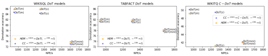
Figure 4: $DoT$ models efficiency accuracy trade-off. The $DoT$ models are displayed according to their accuracy in function of the average number of processed examples par second. The models are faster being closer to the right side of the figures and have higher accuracy being closer to the top. This figure compares the efficiency accuracy trade-off of using different pruning transformers – medium, small and mini – and study the impact of $HEM$ and $CC$ on $DoT$. We use token selection for both WIKISQL and TabFact and column selection for WIKITQ.

Effects of $HEM$ and $CC$ on $DoT$

Table 1 and Figure 4 compare the effect of using $HEM$ and $CC$ on $DoT$ models. As both heuristics are applied in the pre-processing step, using $HEM$ or $CC$ along with a similar $DoT$ model, doesn’t change the average number of processed examples per second $NPE/s$ computed over the training step. For both WIKISQL and TabFact we use a token based selection to select the top-$K$ tokens. Combining the token based strategy with $HEM$, outperforms on accuracy the token pruning $DoT$ combined with $CC$. For WIKITQ, the top-$K$ pruning is a column based selection. Unlike the token selection the column pruning combined with $HEM$ gives a lower accuracy.

6 Related work

Efficient Transformers

Improving the computational efficiency of transformer models, especially for serving, is an active research topic. Proposed approaches fall into four categories. The first is to use knowledge distillation, either during the pre-training phase Sanh et al. (2019), or for building task-specific models Sun et al. (2019), or for both Jiao et al. (2020). The second category is to use quantization-aware training during the fine-tuning phase of BERT models, such as Zafrir et al. (2019). The third category is to modify the transformer architecture to improve the dependence on the sequence length Choromanski et al. (2020); Wang et al. (2020). The fourth category is to use pruning strategies such as McCarley (2019), who studied structured pruning to reduce the number of parameters in each transformer layer, and Fan et al. (2020) who used structured dropout to reduce transformer depth at inference time. Our method most closely resembles the last category, but we focus our efforts on shrinking the sequence length of the input instead of model weights. Eisenschlos et al. (2020) explore heuristic methods based on lexical overlap and apply it to tasks involving tabular data, as we do, but our algorithm is learned end-to-end and more general in nature.

Interpretable NLP

Another related line of work attempts to interpret neural networks by searching for rationales Lei et al. (2016), which are a subset of words in the input text that serve as a justification for the prediction. Lei et al. (2016) learn the rationale as a latent discrete variable inside a computation graph with the reinforce method Williams (1992). Bastings et al. (2019) propose instead using stochastic computation nodes and continuous relaxations Maddison et al. (2017), based on re-parametrization Diederik and Max (2014) to approximate the discrete choice of a rationale from an input text, before using it as input for a classifier. Partially masked tokens are then replaced at the input embedding layer by some linear interpolation. We rely on a soft attention mask instead as a way to partially reduce the information coming from some tokens during training. To the best of our knowledge these methods have not been investigated in the context of semi-structured data such as tables or evaluated with a focus on efficiency.

7 Conclusion

We introduced double transformer ($DoT$) where an additional small model prunes the input of a larger second model. This accelerates the training and inference time at a low drop in accuracy. As future work we will explore hierarchical pruning and adapt $DoT$ to other semi-structured NLP tasks.

Appendix

Appendix A $DoT$ model

A.1 Attention scores defines the meaning of relevant tokens.

We study, the updates of the pruning scores according to the attention scores needs. We note the set of relevant tokens $R$. The output probability given by the pruning transformer is in $(0,1)$ making $s_{t}$ in $(-\infty,0)$. Lets suppose that the token $t$ is not needed to answer the question, then the attention scores are decreased $z^{<i,t,t^{\prime}>|s_{t}}\to\vec{-\infty}$ for all the tokens $t^{\prime}\in R$ for all the layers $i$. The model updates both parts of $z^{<i,t,t^{\prime}>}$ making $s_{t}$ converging to $-\infty$, then $\lim_{s_{t}\to-\infty}z^{<i,t,t^{\prime}>|s_{t}}=\vec{-\infty}$. Thus, the meaning of relevant token is defined by the attention scores updates: The pruning scores decreases for non relevant tokens and increase for relevant ones.

A.2 $DoT$ loss

The $DoT$ loss is similar to TAPAS model loss – noted as $J_{SA}=J_{aggr}+\beta J_{scalar}$ in Herzig et al. (2020) – computed over the task-specific transformer where the attention scores are modified. More precisely, we modify only the scalar loss of the task specific model $J_{scalar}$. We incorporate the pruning scores $S=\{s_{t}\forall t\in T_{top_{k}=256}\}$, and we note $J_{scalar|S}$. The $DoT$ loss is then compute only over the top-$K$ tokens: $J_{DoT}=J_{aggr}+\beta J_{scalar|S}$.

For TabFact dataset, Eisenschlos et al. (2020) modified the TAPAS loss – used for QA tasks – to adapt it to the entailment task: Aggregation is not used, instead, one hidden layer is added as output of the [CLS] token to compute the probability of Entailment. We use a similar loss for TabFact where the attention scores are modified.

A.3 Feed-forward pass: Safe use of shorter inputs for the task-specific transformer

The top-$K$ selection enables the use of shorter inputs for the task-specific. We prove that using input length equal to K is equivalent to using input length higher than K, without any loss of context. Note that the pruning scores are the same for both inputs, where the top-$K$ are scored non-zero and we impose the other tokens to be scored zero.

Theorem A.1.

Given a transformer and a set of tokens as input $I$. Let $t$ be one of the input tokens $t\in I$. If the transformer verifies the following conditions, that holds for all layers $i$.

1. $\forall t^{\prime}\in I$ that attends to $t$, , $z^{<i,t,t^{\prime}>}=\vec{-\infty}$.

2. For $t$ attends to any $t^{\prime}\in I$, $z^{<i,t^{\prime},t>}=\vec{-\infty}$.

Then applying this transformer on $I$ is equivalent to applying it on $I-\{t\}$

Proof.

We look at the different use cases.

$\forall i$ layers, any token $t^{\prime}\in I-\{t\}$ attending to any token $t^{\prime\prime}\in I-\{t\}$: the soft-max scores $a^{<i,t^{\prime},t^{\prime\prime}>}$ have the same formula using $I$ or $I-\{t\}$ as input.

Lets fix $t^{\prime}=t$. The token $t$ attending to any token $t^{\prime\prime}\in I$: The first condition 1 gives $\forall t^{\prime\prime}$ that attends to $t$, $z^{<i,t,t^{\prime\prime}>}=\vec{-\infty}$. That follows $exp(z^{<i,t,t^{\prime\prime}>})=\vec{0}$ then $a^{<i,t,t^{\prime\prime}>}=\vec{0}$.

Similarly, if $t^{\prime}=t$. Any token $t^{\prime\prime}\in I$ attending to $t$: The second condition 2 gives $\forall t^{\prime}$ that attends to $t$, $z^{<i,t,t^{\prime\prime}>}=\vec{-\infty}$. That follows $exp(z^{<i,t^{\prime},t>})=\vec{0}$ then $a^{<i,t^{\prime},t>}=\vec{0}$. ∎

Remark.

Given a transformer and a set of tokens as input $I$. Let $t$ be one of the input tokens $t\in I$ with $t$ is not selected by the pruning transformer scored zero – not the first-k tokens. Using $DoT$, $s_{t}=-\infty$. That follows $z^{<i,t,t^{\prime}>}=\vec{-\infty}$.

The case $t^{\prime}=t$, for any token $t^{\prime\prime}\in I$ attending to $t$ we have: $\forall i\neq 0$, the input $E_{t}=\sum_{t^{\prime\prime}\in I}a^{<i,t,t^{\prime\prime}>}$. As $z^{<i,t,t^{\prime}>}=\vec{-\infty}$, $E_{t}=\vec{0}$, $E_{t}$ zero out all the variables making $exp(z^{<i,t^{\prime},t>})$ a constant and $a^{<i,t^{\prime},t>}$ independent of $t^{\prime}$. This is equivalent to $\forall i\neq 0$, $t$ doesn’t attend to any $t^{\prime}\in I$.

Only for the first layer $i=0$, we add an approximation to drop the attention ($t$ attending to $t^{\prime}\in I$). We consider the impact of $t$ on the full attention is small as we stuck multiple layers. We experimented with a task-specific model with a big input length $>k$ and compare it to a task-specific model with input length $=k$. The two models gives similar accuracy. In our experiment we report only the results for the model with input length $=k$.

This makes the attention scores similar to the ones computed over $t\notin I$.

Appendix B Experiments

In all the experiment we report the median accuracy and the error margin computed over 3 runs. We estimate the error margin as half the inter quartile range, that is half the difference between the $25^{th}$ and $75^{th}$ percentiles.

B.1 Models hyper-parameters

We do not perform hyper-parameters search for $DoT$ models we use the same as TAPAS baselines. For WIKISQL and WIKITQ we use the same hyper-parameters as the one used by Herzig et al. (2020) and for TabFact the one used by Eisenschlos et al. (2020). Baselines and $DoT$ are initialized from models pre-trained with a MASK-LM task and on SQAIyyer et al. (2017) following Herzig et al. (2020).

We report the models hyper parameters used for TAPAS baselines and $DoT$ in Table 4. The hyper-parameters are fixed independently of the pre-processing step or the input size: For all the pre-processing input lengths – $\{256,512,1024\}$–, for both $CC$ and $HEM$ we use the same hyper-parameters. Additionally, we use an Adam optimizer with weight decay for all the baselines and $DoT$ models –the same configuration as BERT.

Dataset	lr	$\rho$	hidden dropout	attention dropout	num steps
WIKISQL	$6e^{-5}$	$0.14$	$0.1$	$0.1$	$50,000$
TabFact	$2e^{-5}$	$0.05$	$0.07$	$0.0$	$80,000$
WIKITQ	$1.9e^{-5}$	$0.19$	$0.1$	$0.1$	$50,000$

Table 4: Hyper-parameters used per dataset. Reports the learning rate (lr), the warmup ratio ($\rho$), the hidden dropout, the attention dropout and the number of training steps (num steps) used for each dataset. These hyper-parameters are the same for all the baselines and $DoT$ models.

B.2 state-of-the-art

We report state-of-the-art for the three datasets in Table 5.

Model	test accuracy
Agarwal et al. (2019) MeRL	$74.8\pm 0.2$
Liang et al. (2018) MAPO (ensemble of 10)	$74.9$
Wang et al. (2019)	$79.3$
$CC\xrightarrow[]{512}\textsc{TAPAS}(l)$Herzig et al. (2020)	$83.6$
Min et al. (2019)	$83.9$

(a) state-of-the-art WIKISQL

Model	test accuracy
Zhong et al. (2020) LFC (LPA)	$71.6$
Zhong et al. (2020) LFC (Seq2Action)	$71.7$
Shi et al. (2020) HeterTFV	$72.3$
Zhang et al. (2020) SAT	$73.2$
Yang et al. (2020) ProgVGAT	$74.4$
$CC\xrightarrow[]{512}\textsc{TAPAS}(l)$ Eisenschlos et al. (2020)	$81.0$

(b) state-of-the-art TabFact

Model	test accuracy
Agarwal et al. (2019) MeRL	$44.1\pm 0.2$
Dasigi et al. (2019) Iterative Search (best)	$44.3$
Wang et al. (2019)	$44.5$
Liang et al. (2018) MAPO (ensembled-$10$)	$46.3$
Agarwal et al. (2019) MeRL ensemble of $10$ models	$46.9$
$CC\xrightarrow[]{512}\textsc{TAPAS}(l)$Herzig et al. (2020)	$48.8$
Yin et al. (2020) $MAPO+TABERT(l)(K=3)$	$51.8\pm 0.6$

(c) state-of-the-art WIKITQ

Table 5: state-of-the-art accuracy on test set.

B.3 Models complexity

In all our experiments we use different transformer sizes called large, medium, small and mini. These models correspond to the BERT open sourced model sizes described in Turc et al. (2019). We report all models complexity in Table 6.

Model	$\#L$	$H$	$\#Hs$	$Hi$
large	$24$	$1024$	$16$	$4096$
medium	$8$	$512$	$8$	$2048$
small	$4$	$512$	$8$	$2048$
mini	$4$	$256$	$4$	$1024$

Table 6: Models complexity with $\#L$ is the number of layers, $\#Hs$ the number of heads, $H$ the embedding size and $Hi$ the intermediate size.

The sequence length changes the total number of used parameters. The formula to count the number of parameters is given by Table 7.

Num layers $\times$ Module	Tensor	Shape
$1\times$Embedding	embeddings.word_embeddings	$[V,H]$
	embeddings.position_embeddings	$[I,H]$
	embeddings.token_type_embeddings	$[3,H]$
		$+[2,H]$
		$+[10,H]$
		$+4[256,H]$
	embeddings.LayerNorm	$[H]$
		$+[I]$
$L\times$Transformer	encoder.layer.0.attention.self.query.kernel	$[I,H]$
	encoder.layer.0.attention.self.query.bias	$[H]$
	encoder.layer.0.attention.self.key.kernel	$[I,H]$
	encoder.layer.0.attention.self.key.bias	$[H]$
	encoder.layer.0.attention.self.value.kernel	$[I,H]$
	encoder.layer.0.attention.self.value.bias	$[H]$
	encoder.layer.0.attention.output.dense.kernel	$[H,H]$
	encoder.layer.0.attention.output.dense.bias	$[H]$
	encoder.layer.0.attention.output.LayerNorm	$[H]$
		$+[H]$
	encoder.layer.0.intermediate.dense.kernel	$[H,Hi]$
	encoder.layer.0.intermediate.dense.bias	$[Hi]$
	encoder.layer.0.output.dense.kernel	$[Hi,H]$
	encoder.layer.0.output.dense.bias	$[H]$
	encoder.layer.0.output.LayerNorm	$[H]$
		$+[H]$
$1\times$ Pooler	pooler.dense.kernel	$[I,H]$
	pooler.dense.bias	$[H]$

Table 7: Parameters counts. Let $H$ be the hidden embedding size, $L$ the number of layers, $Hi$ the intermediate size, $V=30522$ the vocabulary size and $I$ the input size. We report the used parameters based on tensors shape for TAPAS models.

The number of used parameters equals to $V\times H+(2+3L)I\times H+I+(256*4+17+9L)H+(1+2L\times H)\times Hi$. The number of parameters of each model is reported in Table 8

Model	Parameters count
	$CC\xrightarrow[]{256}$	$CC\xrightarrow[]{512}$	$CC\xrightarrow[]{1024}$
$\mbox{TAPAS}(mini)$	$11.1M$	$12.0M$	$13.8M$
$\mbox{TAPAS}(s)$	$26.4M$	$28.2M$	$31.9M$
$\mbox{TAPAS}(m)$	$36.3M$	$39.7M$	$46.6M$
$\textsc{TAPAS}(l)$	$253.2M$	$272.6M$	$311.4M$
$DoT(mini\xrightarrow[]{256}l)$	$264.3M$	$265.3M$	$267.1M$
$DoT(s\text{ }\xrightarrow[]{256}l)$	$279.6M$	$281.5M$	$285.1M$
$DoT(m\xrightarrow[]{256}l)$	$289.6M$	$293M$	$299.8M$

Table 8: The parameters count for the different models. $M$ refers to millions. The number of parameters is the same using $HEM$ or $CC$. The column based $DoT$ models have the same number of parameters than the token based $DoT$ models.

The number of parameters is not proportional to the computational time as multiple operations involves multiplying tensors of shapes $[I,H]\times[H,H]$.

Appendix C Analysis

We report additional results for the analysis.

C.1 Pruning transformer enables reaching high accuracy for long input sequences

To study the model accuracy on different input sequence lengths, we bucketize the datasets. Table 9 reports the accuracy results computed over the test set for all buckets. We use $DoT(m\xrightarrow[]{256}l)$ model for the three datasets, a token based pruning for both WIKISQL and TabFact and a column based pruning for WIKISQL. For a length $>1024$, the $DoT$ model outperforms the $256$ and $512$ length baselines for all tasks. For the bucket $[512,1024]$, $DoT$ model gives close results to $512$ length baseline. This indicates that the pruning model extracts twice more relevant tokens than the heuristic $CC$. For smaller input lengths the baseline models outperform $DoT$. One cause could be the hyper-parameters tuning as we do not tune the hyper parameters for $DoT$.

Bucket	Model	WIKISQL	TabFact	WIKITQ
$>1024$	$\text{ }CC\xrightarrow[]{1024}\textsc{TAPAS}(l)$	$54.7\pm 1.0$	$74.1\pm 1.5$	$30.7\pm 0.9$
	$\text{ }CC\>\>\xrightarrow[]{512}\textsc{TAPAS}(l)$	$24.3\pm 0.1$	$56.8\pm 2.2$	$18.8\pm 0.9$
	$\text{ }CC\>\>\xrightarrow[]{256}\textsc{TAPAS}(l)$	$5.8\pm 0.2$	$9.9\pm 1.5$	$6.9\pm 0.0$
	$\text{ }CC\xrightarrow[]{1024}DoT(m\xrightarrow[]{256}l)$	$40.1\pm 4.9$	$69.1\pm 2.5$	$23.8\pm 0.5$
$[512,1024]$	$\text{ }CC\xrightarrow[]{1024}\textsc{TAPAS}(l)$	$86.1\pm 0.5$	$78.0\pm 0.4$	$48.2\pm 0.1$
	$\text{ }CC\>\>\xrightarrow[]{512}\textsc{TAPAS}(l)$	$73.6\pm 0.1$	$73.0\pm 0.3$	$42.7\pm 0.6$
	$\text{ }CC\>\>\xrightarrow[]{256}\textsc{TAPAS}(l)$	$40.9\pm 0.3$	$43.9\pm 0.4$	$18.6\pm 0.1$
	$\text{ }CC\xrightarrow[]{1024}DoT(m\xrightarrow[]{256}l)$	$72.9\pm 1.8$	$74.7\pm 0.7$	$39.1\pm 0.6$
$[256,512]$	$\text{ }CC\xrightarrow[]{1024}\textsc{TAPAS}(l)$	$87.0\pm 0.0$	$80.3\pm 0.2$	$56.1\pm 0.4$
	$\text{ }CC\>\>\xrightarrow[]{512}\textsc{TAPAS}(l)$	$88.2\pm 0.1$	$81.1\pm 0.2$	$56.5\pm 1.1$
	$\text{ }CC\>\>\xrightarrow[]{256}\textsc{TAPAS}(l)$	$78.5\pm 0.7$	$71.4\pm 0.3$	$50.2\pm 0.8$
	$\text{ }CC\xrightarrow[]{1024}DoT(m\xrightarrow[]{256}l)$	$86.4\pm 0.7$	$78.4\pm 0.5$	$53.1\pm 0.5$
$<256$	$\text{ }CC\xrightarrow[]{1024}\textsc{TAPAS}(l)$	$87.7\pm 0.0$	$82.2\pm 0.1$	$58.7\pm 0.2$
	$\text{ }CC\>\>\xrightarrow[]{512}\textsc{TAPAS}(l)$	$88.2\pm 0.3$	$83.2\pm 0.0$	$60.2\pm 1.0$
	$\text{ }CC\>\>\xrightarrow[]{256}\textsc{TAPAS}(l)$	$88.4\pm 1.1$	$82.1\pm 0.2$	$59.1\pm 0.7$
	$\text{ }CC\xrightarrow[]{1024}DoT(m\xrightarrow[]{256}l)$	$87.8\pm 0.2$	$79.9\pm 0.5$	$57.3\pm 0.6$

Table 9: The denotation accuracy for test, computed over bucketized datasets per sequence length.

C.2 Choice of joint learning: Is it better to impose the meaning of relevant tokens?

According to the analysis done in Section 5, the pruning model –jointly learned– is selecting the tokens to solve the main task. This raises a question of whether adding a pruning loss similar to the task-specific loss can improve the end-to-end accuracy. We not $J_{pruning-scalar}$ the pruning loss and $J_{task-specific-scalar}$ the task-specific loss. Both are similar to $J_{scalar}$ defined by Herzig et al. (2020) where the attention scores are not affected by the pruning scores. We additionally not $J_{task-specific-scalar|S}$ the task specific loss affected by the set of pruning scores $S$.

We compare the joint learning model $J\mbox{-}DoT(.)$ – defined in Appendix A.2 – to a model learned using an additional pruning loss $P\mbox{-}DoT(.)=J_{aggr}+\beta(J_{task-specific-scalar}+J_{pruning-scalar})$, and another using both $PJ\mbox{-}DoT(.)=J_{aggr}+\beta(J_{task-specific-scalar|S}+J_{pruning-scalar})$. Table 10 shows that for both WIKISQL and WIKITQ joint learning achieves higher accuracy for similar efficiency. For TabFact the median is in the margin error but the best model using the joint learning outperforms the other learning strategies.

Dataset	WIKISQL			TabFact			WIKITQ
Model	test accuracy	Best	$NPE/s$	test accuracy	Best	$NPE/s$	test accuracy	Best	$NPE/s$
$CC\xrightarrow[]{1024}P\mbox{-}DoT(m\xrightarrow[]{256}l)$	$80.4\pm 0.6$	$82.11$	$950$	$79.7\pm 0.5$	$80.20$	$930$	$43.5\pm 0.6$	$44.54$	$950$
$CC\xrightarrow[]{1024}PJ\mbox{-}DoT(m\xrightarrow[]{256}l)$	$82.9\pm 0.6$	$83.21$	$950$	$78.0\pm 0.3$	$78.41$	$930$	$46.4\pm 0.8$	$48.43$	$950$
$CC\xrightarrow[]{1024}J\mbox{-}DoT(m\xrightarrow[]{256}l)$	$83.6\pm 0.5$	$84.67$	$950$	$79.0\pm 0.5$	$81.28$	$930$	$50.1\pm 0.5$	$50.14$	$950$

Table 10: Test denotation accuracy using different $DoT$ training losses. We compare a joint learning $J\mbox{-}DoT$ model – that enables the back propagation of the pruning transformer by modifying the attention scores – to two different $DoT$ models where we modify the learning strategy. $P\mbox{-}DoT$ disables the buck-propagation to the pruning transformer through the attention scores, instead it uses an additional pruning loss similar to the task-specific loss. The second strategy, $JP\mbox{-}DoT$ is a hybrid method where the joint learning is used along with an additional pruning loss. $J\mbox{-}DoT$ achieves higher accuracy for similar efficiency, for both WIKISQL and WIKITQ. For TabFact the median is in the margin error but the best model using the joint learning outperforms the other learning strategies.

Appendix D All models results

We report all $DoT$ results in Table 11. $C-DoT$ indicates the column based selection: For each token from one column, the pruning score attributes a column score instead of a token score. The column score is computed as an average of its tokens’ scores.

Dataset	WIKISQL			TabFact			WIKITQ
Model	test accuracy	Best	NPE/s	test accuracy	Best	NPE/s	test accuracy	Best	NPE/s
state-of-the-art	$83.9$	$-$	$-$	$81.0$	$-$	$-$	$51.8\pm 0.6$	$52.3$	$-$
$\text{\ \ \ \ }CC\xrightarrow[]{1024}\mbox{TAPAS}(s)$	$74.6\pm 0.1$	$74.69$	$3900$	$73.3\pm 0.1$	$73.40$	$4400$	$36.0\pm 0.4$	$36.92$	$3800$
$\text{\ \ \ \ }CC\xrightarrow[]{1024}\mbox{TAPAS}(m)$	$81.6\pm 0.2$	$81.55$	$2050$	$75.1\pm 0.2$	$75.75$	$2300$	$42.9\pm 0.3$	$43.67$	$2020$
$\text{\ \ \ \ }CC\text{ }\xrightarrow[]{256}\textsc{TAPAS}(l)$	$76.4\pm 0.3$	$77.15$	$1870$	$75.1\pm 0.3$	$76.13$	$1900$	$44.8\pm 0.5$	$45.47$	$1900$
$\text{\ \ \ \ }CC\text{ }\xrightarrow[]{512}\textsc{TAPAS}(l)$	$83.6\pm 0.1$	$83.65$	$800$	$81.3\pm 0.2$	$81.60$	$870$	$52.2\pm 0.5$	$52.74$	$810$
$\text{\ \ \ \ }CC\xrightarrow[]{1024}\textsc{TAPAS}(l)$	$86.0\pm 0.3$	$86.6$	$270$	$81.6\pm 0.1$	$81.64$	$300$	$53.9\pm 0.2$	$54.30$	$270$
$HEM\xrightarrow[]{256}\textsc{TAPAS}(l)$	$77.4\pm 0.3$	$77.97$	$1870$	$75.5\pm 0.2$	$75.80$	$1900$	$47.3\pm 0.1$	$47.70$	$1900$
$HEM\text{ }\xrightarrow[]{512}\textsc{TAPAS}(l)$	$83.8\pm 0.4$	$84.75$	$800$	$82.0\pm 0.3$	$82.07$	$870$	$52.7\pm 0.4$	$53.61$	$810$
$HEM\xrightarrow[]{1024}\textsc{TAPAS}(l)$	$85.9\pm 0.0$	$85.94$	$270$	$80.6\pm 0.0$	$80.6$	$300$	$54.0\pm 0.9$	$54.93$	$270$
$\text{\ \ \ \ }CC\xrightarrow[]{1024}DoT(mini\xrightarrow[]{256}l)$	$72.8\pm 0.8$	$73.01$	$1600$	$77.2\pm 0.5$	$77.72$	$1670$	$37.4\pm 0.9$	$39.48$	$1600$
$\text{\ \ \ \ }CC\xrightarrow[]{1024}DoT(s\text{ }\xrightarrow[]{256}l)$	$74.2\pm 3.6$	$84.27$	$1250$	$81.0\pm 0.1$	$81.17$	$1300$	$40.8\pm 0.4$	$42.15$	$1250$
$\text{\ \ \ \ }CC\xrightarrow[]{1024}DoT(m\xrightarrow[]{256}l)$	$83.6\pm 0.5$	$84.67$	$950$	$79.0\pm 0.5$	$81.28$	$930$	$42.4\pm 0.5$	$43.44$	$950$
$HEM\xrightarrow[]{1024}DoT(mini\text{ }\xrightarrow[]{256}l)$	$73.4\pm 0.1$	$73.70$	$1600$	$77.6\pm 0.2$	$78.19$	$1670$	$39.2\pm 0.3$	$39.8$	$1600$
$HEM\xrightarrow[]{1024}DoT(s\text{ }\xrightarrow[]{256}l)$	$85.3\pm 0.4$	$85.76$	$1250$	$81.6\pm 0.3$	$81.74$	$1300$	$42.1\pm 0.7$	$42.15$	$1250$
$HEM\xrightarrow[]{1024}DoT(m\xrightarrow[]{256}l)$	$85.5\pm 0.2$	$85.82$	$950$	$81.8\pm 0.0$	$81.94$	$930$	$48.2\pm 1.8$	$48.46$	$950$
$\text{\ \ \ \ }CC\xrightarrow[]{1024}C-DoT(mini\text{ }\xrightarrow[]{256}l)$	$72.0\pm 1.1$	$74.06$	$1560$	$77.3\pm 4.8$	$77.61$	1600	$41.0\pm 0.4$	$42.13$	$1560$
$\text{\ \ \ \ }CC\xrightarrow[]{1024}C-DoT(s\text{ }\xrightarrow[]{256}l)$	$74.3\pm 0.1$	$74.49$	$1250$	$77.2\pm 4.9$	$78.04$	$1300$	$48.1\pm 2.4$	$49.47$	$1250$
$\text{\ \ \ \ }CC\xrightarrow[]{1024}C-DoT(m\xrightarrow[]{256}l)$	$73.9\pm 0.2$	$7454$	$950$	$78.3\pm 0.7$	$80.12$	$930$	$50.1\pm 0.5$	$50.14$	$950$
$HEM\xrightarrow[]{1024}C-DoT(mini\text{ }\xrightarrow[]{256}l)$	$72.0\pm 1.1$	$74.06$	$1560$	$78.1\pm 4.8$	$78.13$	1600	$41.5\pm 0.1$	$41.99$	$1560$
$HEM\xrightarrow[]{1024}C-DoT(s\text{ }\xrightarrow[]{256}l)$	$74.5\pm 0.8$	$74.72$	$1250$	$58.5\pm 0.3$	$59.19$	$1300$	$40.9\pm 0.2$	$41.23$	$1250$
$HEM\xrightarrow[]{1024}C-DoT(m\xrightarrow[]{256}l)$	$74.3\pm 2.1$	$74.56$	$950$	$77.3\pm 0.1$	$77.71$	$930$	$40.1\pm 2.4$	$49.13$	$950$

Table 11: Summary of all the experiments’ results on the accuracy efficiency trade-off. The state-of-the-art (detailed in Appendix B.2) correspond to the values of Min et al. (2019) for WIKISQL, Eisenschlos et al. (2020) for TabFact and Yin et al. (2020) for WIKITQ. For each dataset, the state-of-the-art, the best baseline model on accuracy, and the $DoT$ models that reach the best accuracy efficiency trade-off are highlighted.

References

- Agarwal et al. (2019) Rishabh Agarwal, Chen Liang, Dale Schuurmans, and Mohammad Norouzi. 2019. Learning to generalize from sparse and underspecified rewards. In Proceedings of the 36th International Conference on Machine Learning, volume 97 of Proceedings of Machine Learning Research, pages 130–140. PMLR.
- Bastings et al. (2019) Jasmijn Bastings, Wilker Aziz, and Ivan Titov. 2019. Interpretable neural predictions with differentiable binary variables. In Proceedings of the 57th Annual Meeting of the Association for Computational Linguistics, pages 2963–2977, Florence, Italy. Association for Computational Linguistics.
- Choromanski et al. (2020) Krzysztof Choromanski, Valerii Likhosherstov, David Dohan, Xingyou Song, Andreea Gane, Tamás Sarlós, Peter Hawkins, Jared Davis, Afroz Mohiuddin, Lukasz Kaiser, David Belanger, Lucy Colwell, and Adrian Weller. 2020. Rethinking attention with performers. CoRR, abs/2009.14794.
- Dasigi et al. (2019) Pradeep Dasigi, Matt Gardner, Shikhar Murty, Luke Zettlemoyer, and Eduard Hovy. 2019. Iterative search for weakly supervised semantic parsing. In Proceedings of the 2019 Conference of the North American Chapter of the Association for Computational Linguistics: Human Language Technologies, Volume 1 (Long and Short Papers), pages 2669–2680, Minneapolis, Minnesota. Association for Computational Linguistics.
- De Cao et al. (2020) Nicola De Cao, Michael Sejr Schlichtkrull, Wilker Aziz, and Ivan Titov. 2020. How do decisions emerge across layers in neural models? interpretation with differentiable masking. In Proceedings of the 2020 Conference on Empirical Methods in Natural Language Processing (EMNLP), pages 3243–3255, Online. Association for Computational Linguistics.
- Devlin et al. (2019) Jacob Devlin, Ming-Wei Chang, Kenton Lee, and Kristina Toutanova. 2019. BERT: Pre-training of deep bidirectional transformers for language understanding. In Proceedings of the 2019 Conference of the North American Chapter of the Association for Computational Linguistics: Human Language Technologies, Volume 1 (Long and Short Papers), pages 4171–4186, Minneapolis, Minnesota. Association for Computational Linguistics.
- Diederik and Max (2014) P. Kingma Diederik and Welling Max. 2014. Auto-encoding variational bayes. In International Conference on Learning Representations, ICLR 2014, Banff, Canada.
- Eisenschlos et al. (2020) Julian Eisenschlos, Syrine Krichene, and Thomas Müller. 2020. Understanding tables with intermediate pre-training. In Findings of the Association for Computational Linguistics: EMNLP 2020, pages 281–296, Online. Association for Computational Linguistics.
- Fan et al. (2020) Angela Fan, Edouard Grave, and Armand Joulin. 2020. Reducing transformer depth on demand with structured dropout. In International Conference on Learning Representations ICLR 2020, Virtual Conference, Formerly Addis Ababa ETHIOPIA.
- Herzig et al. (2020) Jonathan Herzig, Pawel Krzysztof Nowak, Thomas Müller, Francesco Piccinno, and Julian Eisenschlos. 2020. TaPas: Weakly supervised table parsing via pre-training. In Proceedings of the 58th Annual Meeting of the Association for Computational Linguistics, pages 4320–4333, Online. Association for Computational Linguistics.
- Iyyer et al. (2017) Mohit Iyyer, Wen-tau Yih, and Ming-Wei Chang. 2017. Search-based neural structured learning for sequential question answering. In Proceedings of the 55th Annual Meeting of the Association for Computational Linguistics (Volume 1: Long Papers), pages 1821–1831, Vancouver, Canada. Association for Computational Linguistics.
- Jiao et al. (2020) Xiaoqi Jiao, Yichun Yin, Lifeng Shang, Xin Jiang, Xiao Chen, Linlin Li, Fang Wang, and Qun Liu. 2020. TinyBERT: Distilling BERT for natural language understanding. In Findings of the Association for Computational Linguistics: EMNLP 2020, pages 4163–4174, Online. Association for Computational Linguistics.
- Lei et al. (2016) Tao Lei, Regina Barzilay, and Tommi Jaakkola. 2016. Rationalizing neural predictions. In Proceedings of the 2016 Conference on Empirical Methods in Natural Language Processing, pages 107–117, Austin, Texas. Association for Computational Linguistics.
- Liang et al. (2018) Chen Liang, Mohammad Norouzi, Jonathan Berant, Quoc V Le, and Ni Lao. 2018. Memory augmented policy optimization for program synthesis and semantic parsing. In Advances in Neural Information Processing Systems, volume 31. Curran Associates, Inc.
- Liu et al. (2019) Yinhan Liu, Myle Ott, Naman Goyal, Jingfei Du, Mandar Joshi, Danqi Chen, Omer Levy, Mike Lewis, Luke Zettlemoyer, and Veselin Stoyanov. 2019. Roberta: A robustly optimized BERT pretraining approach. CoRR, abs/1907.11692.
- Maddison et al. (2017) Chris J. Maddison, Andriy Mnih, and Yee Whye Teh. 2017. The concrete distribution: A continuous relaxation of discrete random variables. In 5th International Conference on Learning Representations, ICLR 2017, Toulon, France, Conference Track Proceedings.
- McCarley (2019) J. S. McCarley. 2019. Pruning a bert-based question answering model. CoRR, abs/1910.06360.
- Min et al. (2019) Sewon Min, Danqi Chen, Hannaneh Hajishirzi, and Luke Zettlemoyer. 2019. A discrete hard EM approach for weakly supervised question answering. In Proceedings of the 2019 Conference on Empirical Methods in Natural Language Processing and the 9th International Joint Conference on Natural Language Processing (EMNLP-IJCNLP), pages 2851–2864, Hong Kong, China. Association for Computational Linguistics.
- Pasupat and Liang (2015) Panupong Pasupat and Percy Liang. 2015. Compositional semantic parsing on semi-structured tables. In Proceedings of the 53rd Annual Meeting of the Association for Computational Linguistics and the 7th International Joint Conference on Natural Language Processing (Volume 1: Long Papers), pages 1470–1480, Beijing, China. Association for Computational Linguistics.
- Radford et al. (2019) Alec Radford, Jeffrey Wu, Rewon Child, David Luan, Dario Amodei, and Ilya Sutskever. 2019. Language models are unsupervised multitask learners. OpenAI Blog, 1(8):9.
- Sanh et al. (2019) Victor Sanh, Lysandre Debut, Julien Chaumond, and Thomas Wolf. 2019. Distilbert, a distilled version of bert: smaller, faster, cheaper and lighter. The 5th Workshop on Energy Efficient Machine Learning and Cognitive Computing (EMC2) Co-located with NeurIPS 2019, Vancouver, Canada.
- Shi et al. (2020) Qi Shi, Yu Zhang, Qingyu Yin, and Ting Liu. 2020. Learn to combine linguistic and symbolic information for table-based fact verification. In Proceedings of the 28th International Conference on Computational Linguistics, pages 5335–5346, Barcelona, Spain (Online). International Committee on Computational Linguistics.
- Sun et al. (2019) Siqi Sun, Yu Cheng, Zhe Gan, and Jingjing Liu. 2019. Patient knowledge distillation for BERT model compression. In Proceedings of the 2019 Conference on Empirical Methods in Natural Language Processing and the 9th International Joint Conference on Natural Language Processing (EMNLP-IJCNLP), pages 4323–4332, Hong Kong, China. Association for Computational Linguistics.
- Turc et al. (2019) Iulia Turc, Ming-Wei Chang, Kenton Lee, and Kristina Toutanova. 2019. Well-read students learn better: The impact of student initialization on knowledge distillation. CoRR, abs/1908.08962.
- Vaswani et al. (2017) Ashish Vaswani, Noam Shazeer, Niki Parmar, Jakob Uszkoreit, Llion Jones, Aidan N Gomez, Łukasz Kaiser, and Illia Polosukhin. 2017. Attention is all you need. In Advances in Neural Information Processing Systems, volume 30. Curran Associates, Inc.
- Wang et al. (2019) Bailin Wang, Ivan Titov, and Mirella Lapata. 2019. Learning semantic parsers from denotations with latent structured alignments and abstract programs. In Proceedings of the 2019 Conference on Empirical Methods in Natural Language Processing and the 9th International Joint Conference on Natural Language Processing (EMNLP-IJCNLP), pages 3774–3785, Hong Kong, China. Association for Computational Linguistics.
- Wang et al. (2020) Sinong Wang, Belinda Z. Li, Madian Khabsa, Han Fang, and Hao Ma. 2020. Linformer: Self-attention with linear complexity. CoRR, abs/2006.04768.
- Wenhu et al. (2019) Chen Wenhu, Wang Hongmin, Chen Jianshu, Zhang Yunkai, Wang Hong, Li Shiyang, Zhou Xiyou, and Yang Wang William. 2019. Tabfact: A large-scale dataset for table-based fact verification. In International Conference on Learning Representations ICLR 2019, New Orleans.
- Williams (1992) Ronald J. Williams. 1992. Simple statistical gradient-following algorithms for connectionist reinforcement learning. Machine Learning, 8(3–4):229–256.
- Yang et al. (2020) Xiaoyu Yang, Feng Nie, Yufei Feng, Quan Liu, Zhigang Chen, and Xiaodan Zhu. 2020. Program enhanced fact verification with verbalization and graph attention network. In Proceedings of the 2020 Conference on Empirical Methods in Natural Language Processing (EMNLP), pages 7810–7825, Online. Association for Computational Linguistics.
- Yin et al. (2020) Pengcheng Yin, Graham Neubig, Wen-tau Yih, and Sebastian Riedel. 2020. TaBERT: Pretraining for joint understanding of textual and tabular data. In Proceedings of the 58th Annual Meeting of the Association for Computational Linguistics, pages 8413–8426, Online. Association for Computational Linguistics.
- Zafrir et al. (2019) Ofir Zafrir, Guy Boudoukh, Peter Izsak, and Moshe Wasserblat. 2019. Q8bert: Quantized 8bit bert. The 5th Workshop on Energy Efficient Machine Learning and Cognitive Computing (EMC2) Co-located with NeurIPS 2019, Vancouver, Canada.
- Zhang et al. (2020) Hongzhi Zhang, Yingyao Wang, Sirui Wang, Xuezhi Cao, Fuzheng Zhang, and Zhongyuan Wang. 2020. Table fact verification with structure-aware transformer. In Proceedings of the 2020 Conference on Empirical Methods in Natural Language Processing (EMNLP), pages 1624–1629, Online. Association for Computational Linguistics.
- Zhong et al. (2017) Victor Zhong, Caiming Xiong, and Richard Socher. 2017. Seq2sql: Generating structured queries from natural language using reinforcement learning. CoRR, abs/1709.00103.
- Zhong et al. (2020) Wanjun Zhong, Duyu Tang, Zhangyin Feng, Nan Duan, Ming Zhou, Ming Gong, Linjun Shou, Daxin Jiang, Jiahai Wang, and Jian Yin. 2020. LogicalFactChecker: Leveraging logical operations for fact checking with graph module network. In Proceedings of the 58th Annual Meeting of the Association for Computational Linguistics, pages 6053–6065, Online. Association for Computational Linguistics.