Tight Accounting in the Shuffle Model of Differential Privacy

Abstract

Shuffle model of differential privacy is a novel distributed privacy model based on a combination of local privacy mechanisms and a secure shuffler. It has been shown that the additional randomisation provided by the shuffler improves privacy bounds compared to the purely local mechanisms. Accounting tight bounds, however, is complicated by the complexity brought by the shuffler. The recently proposed numerical techniques for evaluating $(\varepsilon,\delta)$-differential privacy guarantees have been shown to give tighter bounds than commonly used methods for compositions of various complex mechanisms. In this paper, we show how to obtain accurate bounds for adaptive compositions of general $\varepsilon$-LDP shufflers using the analysis by Feldman et al. (2021) and tight bounds for adaptive compositions of shufflers of $k$-randomised response mechanisms, using the analysis by Balle et al. (2019). We show how to speed up the evaluation of the resulting privacy loss distribution from $\mathcal{O}(n^{2})$ to $\mathcal{O}(n)$, where $n$ is the number of users, without noticeable change in the resulting $\delta(\varepsilon)$-upper bounds. We also demonstrate looseness of the existing bounds and methods found in the literature, improving previous composition results significantly.

1 Introduction

The shuffle model of differential privacy (DP) is a distributed privacy model which sits between the high trust-high utility centralised DP, and the low trust-low utility local DP (LDP). In the shuffle model, the individual results from local randomisers are only released through a secure shuffler. This additional randomisation leads to “amplification by shuffling”, resulting in better privacy bounds against adversaries without access to the unshuffled local results.

We consider computing privacy bounds for both single and composite shuffle protocols, where by composite protocol we mean a protocol, where the subsequent user-wise local randomisers depend on the same local datasets and possibly on the previous output of the shuffler, and at each round the results from the local randomisers are independently shuffled. Moreover, using the analysis by Feldman et al., (2021), we provide bounds in the case the subsequent local randomisers are allowed to depend adaptively on the output of the previous ones.

In this paper we show how numerical accounting (Koskela et al.,, 2020, 2021; Gopi et al.,, 2021) can be employed for tight privacy analysis of both single and composite shuffle DP mechanisms. To our knowledge, ours is the only existing method enabling tight privacy accounting for composite protocols in the shuffle model. We demonstrate that thus obtained bounds are always tighter than the existing bounds from the literature.

By using the tight privacy bounds we can also evaluate how significantly adversaries with varying capabilities differ in terms of the resulting privacy bounds. That is, we can quantify the value of information in terms of privacy by comparing tight privacy bounds under varying assumptions.

1.1 Related work

DP was originally defined in the central model assuming a trusted aggregator by Dwork et al., (2006), while the fully distributed LDP was formally introduced and analysed by Kasiviswanathan et al., (2011). Closely related to the shuffle model of DP, Bittau et al., (2017) proposed the Encode, Shuffle, Analyze framework for distributed learning, which uses the idea of secure shuffler for enhancing privacy. The shuffle model of DP was formally defined by Cheu et al., (2019), who also provided the first separation result showing that the shuffle model is strictly between the central and the local models of DP. Another direction initiated by Cheu et al., (2019) and continued, e.g., by Balle et al., (2020); Ghazi et al., (2021) has established a separation between single- and multi-message shuffle protocols.

There exists several papers on privacy amplification by shuffling, some of which are central to this paper. Erlingsson et al., (2019) showed that the introduction of a secure shuffler amplifies the privacy guarantees against an adversary, who is not able to access the outputs from the local randomisers but only sees the shuffled output. Balle et al., (2019) improved the amplification results and introduced the idea of privacy blanket, which we also utilise in our analysis of $k$-randomised response in Section 4. We compare our bounds with those of Balle et al., (2019) in Section 4.1. Feldman et al., (2021) used a related idea of hiding in the crowd to improve on the previous results, while Girgis et al., (2021) generalised shuffling amplification further to scenarios with composite protocols and parties with more than one local sample under simultaneous communication and privacy restrictions. We use some results of Feldman et al., (2021) in the analysis of general LDP mechanisms, and compare our bounds with theirs in Section 3.3. We also calculate privacy bounds in the setting considered by Girgis et al., (2021), namely in the case a fixed subset of users sending contributions to the shufflers are sampled randomly. This can be seen as a subsampled mechanism and we are able to combine the analysis of Feldman et al., (2021), the PLD related subsampling results of Zhu et al., (2021) and FFT accounting to obtain tighter $(\varepsilon,\delta)$-bounds than Girgis et al., (2021), as shown in Section 3.4.

2 Background

Before analysing the shuffled mechanisms we need to introduce some theory and notations. With apologies for conciseness, we start by defining DP and PLD, and finish with the Fourier accountant. For more details, we refer to (Koskela et al.,, 2021; Gopi et al.,, 2021; Zhu et al.,, 2021).

2.1 Differential privacy and privacy loss distribution

An input data set containing $n$ data points is denoted as $X=(x_{1},\ldots,x_{n})\in\mathcal{X}^{n}$, where $x_{i}\in\mathcal{X}$, $1\leq i\leq n$. We say $X$ and $X^{\prime}$ are neighbours if we get one by substituting one element in the other (denoted $X\sim X^{\prime}$).

Definition 1.

Let $\varepsilon>0$ and $\delta\in[0,1]$. Let $P$ and $Q$ be two random variables taking values in the same measurable space $\mathcal{O}$. We say that $P$ and $Q$ are $(\varepsilon,\delta)$-indistinguishable, denoted $P\simeq_{(\varepsilon,\delta)}Q$, if for every measurable set $E\subset\mathcal{O}$ we have

$$\mathrm{Pr}(P\in E)\leq{\rm e}\hskip 1.0pt^{\varepsilon}\mathrm{Pr}(Q\in E)+\delta,$$

$$\mathrm{Pr}(Q\in E)\leq{\rm e}\hskip 1.0pt^{\varepsilon}\mathrm{Pr}(P\in E)+\delta.$$

Definition 2.

Let $\varepsilon>0$ and $\delta\in[0,1]$. Mechanism $\mathcal{M}\,:\,\mathcal{X}^{n}\rightarrow\mathcal{O}$ is $(\varepsilon,\delta)$-DP if for every $X\sim X^{\prime}$: $\mathcal{M}(X)\simeq_{(\varepsilon,\delta)}\mathcal{M}(X^{\prime})$. We call $\mathcal{M}$ tightly $(\varepsilon,\delta)$-DP, if there does not exist $\delta^{\prime}<\delta$ such that $\mathcal{M}$ is $(\varepsilon,\delta^{\prime})$-DP. The case when $n=1$ and $\delta=0$ is called $\varepsilon$-LDP.

Tight DP bounds can also be characterised as

$$\delta(\varepsilon)=\max_{X\sim X^{\prime}}\{H_{{\rm e}\hskip 1.0pt^{\varepsilon}}(\mathcal{M}(X)||\mathcal{M}(X^{\prime})),H_{{\rm e}\hskip 1.0pt^{\varepsilon}}(\mathcal{M}(X^{\prime})||\mathcal{M}(X))\},$$

where for $\alpha>0$ the Hockey-stick divergence is defined as

$$H_{\alpha}(P||Q)=\int\max\{0,P(t)-\alpha\cdot Q(t)\}\,\hskip 1.0pt{\rm d}\hskip 0.5ptt.$$

We can generally find tight $(\varepsilon,\delta)$-bounds by analysing a tightly dominating pair of random variables or distributions:

Definition 3 (Zhu et al., 2021).

A pair of distributions $(P,Q)$ is a dominating pair of distributions for mechanism $\mathcal{M}(X)$ if for all neighbouring datasets $X$ and $X^{\prime}$ and for all $\alpha>0$,

$$H_{\alpha}(\mathcal{M}(X)||\mathcal{M}(X^{\prime}))\leq H_{\alpha}(P||Q).$$

If the equality holds for all $\alpha$ for some $X,X^{\prime}$, then $(P,Q)$ is tightly dominating.

We analyse discrete-valued distributions, which means that a dominating pair of distribution $(P,Q)$ can be described by a generalised probability density functions as

$$P(t)=\sum\nolimits_{i}a_{P,i}\cdot\delta_{t_{P,i}}(t),$$ (2.1)

$$Q(t)=\sum\nolimits_{i}a_{Q,i}\cdot\delta_{t_{Q,i}}(t),$$

where $\delta_{t}(\cdot)$, $t\in\mathbb{R}^{d}$, denotes the Dirac delta function centred at $t$, and $t_{P,i},t_{Q,i}\in\mathbb{R}^{d}$ and $a_{P,i},a_{Q,i}\geq 0$. The PLD determined by a pair $(P,Q)$ is defined as follows.

Definition 4.

Let $P$ and $Q$ be generalised probability density functions as defined by (2.1). We define the generalised privacy loss distribution (PLD) $\omega_{P/Q}$ as

$$\omega_{P/Q}(s) =\sum\nolimits_{{t_{P,i}=t_{Q,j}}}a_{P,i}\cdot\delta_{s_{i,j}}(s),\quad s_{i,j}=\log\left(\frac{a_{P,i}}{a_{Q,j}}\right).$$

The following theorem (Zhu et al.,, 2021, Thm. 10) shows that the tight $(\varepsilon,\delta)$-bounds for compositions of adaptive mechanisms are obtained using convolutions of PLDs. The expression (2.2) is equivalent to the hockey-stick divergence $H_{\varepsilon}(P||Q)$ (see e.g. Sommer et al.,, 2019; Koskela et al.,, 2021; Gopi et al.,, 2021).

Theorem 5.

Consider an $n_{c}$-fold adaptive composition given a (tightly) dominating pair $(P,Q)$. The composition is (tightly) $(\varepsilon,\delta)$-DP for $\delta(\varepsilon)$ given by

$$\delta_{P/Q}(\varepsilon)=1-\big{(}1-\delta_{P/Q}(\infty)\big{)}^{n_{c}}+\int\nolimits_{\varepsilon}^{\infty}(1-{\rm e}\hskip 1.0pt^{\varepsilon-s})\left(\omega_{P/Q}*^{n_{c}}\omega_{P/Q}\right)(s)\,\hskip 1.0pt{\rm d}\hskip 0.5pts,$$ (2.2)

$$\delta_{P/Q}(\infty)=\sum\nolimits_{\{t_{i}\,:\,\mathbb{P}(Q=t_{i})=0\}}\mathbb{P}(P=t_{i})$$

and $\omega_{P/Q}*^{n_{c}}\omega_{P/Q}$ denotes the $n_{c}$-fold convolution of the generalised density function $\omega_{P/Q}$.

When computing tight $\delta(\varepsilon)$-bounds for the shufflers of the $k$-RR local randomisers, instead of (2.2), for a certain distribution $\omega$ determined by the shuffler mechanism, we need to evaluate expressions of the form

$$\delta(\varepsilon)=1-\big{(}1-\delta(\infty)\big{)}^{n_{c}}+\int\limits_{\varepsilon}^{\infty}\left(\omega*^{n_{c}}\omega\right)(s)\,\hskip 1.0pt{\rm d}\hskip 0.5pts,$$ (2.3)

where $\delta(\infty)=1-\sum_{i}\omega(i)$. The FFT-based numerical accounting is straightforwardly applied to (2.3) as well.

2.2 Numerical Evaluation of DP Parameters Using FFT

In order to evaluate integrals of the form (2.2) and (2.3) and to find tight privacy bounds, we use the Fast Fourier Transform (FFT)-based method by Koskela et al., (2020, 2021) called the Fourier Accountant (FA). This means that we truncate and place the PLD $\omega$ on an equidistant numerical grid over an interval $[-L,L]$, $L>0$. Convolutions are evaluated using the FFT algorithm and using the error analysis the error incurred by the method can be bounded. We note that alternatively, for accurately computing the integrals and obtaining tight $\delta(\varepsilon)$-bounds, we could also use the FFT-based method proposed by Gopi et al., (2021).

In the next sections we construct the PLD $\omega$ for different shuffling mechanisms. In practice this means that in each case we need a dominating pair of random variables $P$ and $Q$ that then lead to an $(\varepsilon,\delta)$-DP bound.

3 General shuffled $\varepsilon_{0}$-LDP mechanisms

Feldman et al., (2021) consider general $\varepsilon_{0}$-LDP local randomisers combined with a shuffler. The analysis allows also sequential adaptive compositions of the user contributions before shuffling. The analysis is based on decomposing individual LDP contributions to mixtures of data dependent part and noise, which leads to finding $(\varepsilon,\delta)$-bound for the 2-dimensional distributions (see Thm. 3.2 of Feldman et al.,, 2021)

$$P =(A+\Delta,C-A+1-\Delta),$$ (3.1)

$$Q =(A+1-\Delta,C-A+\Delta),$$

where for $n\in\mathbb{N}$,

$$C\sim\mathrm{Bin}(n-1,{\rm e}\hskip 1.0pt^{-\varepsilon_{0}}),\quad A\sim\mathrm{Bin}(C,\tfrac{1}{2}),\quad\Delta\sim\mathrm{Bern}\left(\tfrac{{\rm e}\hskip 1.0pt^{\varepsilon_{0}}}{{\rm e}\hskip 1.0pt^{\varepsilon_{0}}+1}\right).$$

Intuitively, $C$ denotes the number of other users whose mechanism outputs are indistinguishable “clones” of the two different users with $A$ denoting random split between these. Moreover, a numerical method to compute the hockey-stick divergence $H_{{\rm e}\hskip 1.0pt^{\varepsilon}}(P||Q)$ is proposed. Using the results of Zhu et al., (2021) and the following observation, we can use the Fourier accountant to obtain accurate bounds also for adaptive compositions of general $\varepsilon_{0}$-LDP shuffling mechanisms:

Lemma 1.

Let $X$ and $X^{\prime}$ be neighbouring datasets and denote by $\mathcal{A}_{s}(X)$ and $\mathcal{A}_{s}(X^{\prime})$ outputs of the shufflers of adaptive $\varepsilon_{0}$-LDP local randomisers (for more detailed description, see Thm. 3.2 of Feldman et al.,, 2021). Then, for all $\varepsilon>0$,

$$H_{{\rm e}\hskip 1.0pt^{\varepsilon}}(\mathcal{A}_{s}(X)||\mathcal{A}_{s}(X^{\prime}))\leq H_{{\rm e}\hskip 1.0pt^{\varepsilon}}(P||Q),$$

where $P$ and $Q$ are given as in (3.1).

Proof.

By Thm. 3.2 of Feldman et al., (2021) there exists a post-processing algorithm $\Phi$ such that $\Phi(\mathcal{A}_{s}(X))$ is distributed identically to $P$ and $\Phi(\mathcal{A}_{s}(X^{\prime}))$ identically to $Q$. Since in the construction of Thm. 3.2 of Feldman et al., (2021) $X$ and $X^{\prime}$ can be any neighbouring datasets, the claim follows from the post-processing property of DP (see Proposition 2.1 in Dwork and Roth,, 2014). ∎

Using Lemma 46 of Zhu et al., (2021) and the above Lemma 1 yields the following result:

Corollary 2.

The pair of distributions $(P,Q)$ in (3.1) is a dominating pair of distributions for the shuffling mechanism $\mathcal{A}_{s}(X)$.

Furthermore, using Thm. 10 of Zhu et al., (2021), we can bound the $\delta(\varepsilon)$ of $n_{c}$-wise adaptive composition of the shuffler $\mathcal{A}_{s}$ using product distributions of $P$s and $Q$s:

Corollary 3.

Denote $\mathcal{A}^{n_{c}}_{s}(X,z_{0})=\mathcal{A}_{s}(X,\mathcal{A}_{s}(X,...\mathcal{A}_{s}(X,z_{0})))$ for some initial state $z_{0}$. For all neighbouring datasets $X$ and $X^{\prime}$ and for all $\alpha>0$,

$$H_{\alpha}(\mathcal{A}^{n_{c}}_{s}(X)||\mathcal{A}^{n_{c}}_{s}(X^{\prime}))\leq H_{\alpha}(P\times\ldots\times P||Q\times\ldots\times Q),$$ (3.2)

where $P\times\ldots\times P$ and $Q\times\ldots\times Q$ are $n_{c}$-wise product distributions.

The case of heterogeneous adaptive compositions (e.g. for varying $n$ and $\varepsilon_{0}$) can be handled analogously using Thm. 10 of Zhu et al., (2021).

Thus, using (3.2) for $\alpha={\rm e}\hskip 1.0pt^{\varepsilon}$, we get upper bounds for adaptive compositions of general shuffled $\varepsilon_{0}$-LDP mechanisms with the Fourier accountant by finding the PLD for the distributions $P,Q$ (given in Eq. (3.1)). Note that even though the resultsing $(\varepsilon,\delta)$-bound is tight for $P$’s and $Q$’s, it need not be tight for a specific mechanism like the shuffled $k$-RR. The bound simply gives an upper bound for any shuffled $\varepsilon_{0}$-LDP mechanisms. In the Supplements we give also comparisons of the tight bounds obtained with $P$ and $Q$ of (3.1) and with those of the strong $k$-RR adversary (Sec. 4).

3.1 PLD for shuffled $\varepsilon_{0}$-LDP mechanisms

As already noted, we can find $\delta(\varepsilon)$-upper bounds for general shuffled $\varepsilon_{0}$-LDP mechanisms by analysing the pair of distributions $(P,Q)$ of Eq. (3.1). To analyse the compositions, we need to determine the PLD $\omega_{P/Q}$. Since this is straight-forward but the details are messy, we simply state the result here and give the details in the Supplement.

Denoting $q=\frac{{\rm e}\hskip 1.0pt^{\varepsilon_{0}}}{{\rm e}\hskip 1.0pt^{\varepsilon_{0}}+1}$, we see that the distributions in (3.1) are given by the mixture distributions

$$P =q\cdot P_{1}+(1-q)\cdot P_{0},$$

$$Q =(1-q)\cdot P_{1}+q\cdot P_{0},$$

where

$$P_{1}~{}(A+1,C-A),\quad P_{0}~{}(A,C-A+1).$$

In the Supplements we show the following expressions that will determine the PLD.

Lemma 4.

When $b>0$ and $a\geq 0$,

$$\frac{\mathbb{P}(P=(a,b))}{\mathbb{P}(Q=(a,b))}=\frac{q\cdot\frac{a}{b}+(1-q)}{q+(1-q)\frac{a}{b}}.$$

When $0<a\leq n$,

$$\frac{\mathbb{P}(P=(a,0))}{\mathbb{P}(Q=(a,0))}=\frac{q}{1-q}.$$

Lemma 5.

When $a>0$,

$$\mathbb{P}(P_{1}=(a,b))={n-1\choose i}{i\choose j}{\rm e}\hskip 1.0pt^{-i\cdot\varepsilon_{0}}(1-{\rm e}\hskip 1.0pt^{-\varepsilon_{0}})^{n-1-i}\frac{1}{2^{i}},$$

where $(a,b)=(j+1,i-j)$ (i.e., $C=i$ and $A=j$), and

$$\mathbb{P}(P_{0}=(a,b))=\frac{{\rm e}\hskip 1.0pt^{-\varepsilon_{0}}}{1-{\rm e}\hskip 1.0pt^{-\varepsilon_{0}}}\frac{n-a-b}{2a}\mathbb{P}(P_{1}=(a,b)).$$

For $0<b\leq n$, $\mathbb{P}(P_{1}=(0,b))=0$ and

$$\mathbb{P}(P_{0}=(0,b))={n-1\choose b-1}\left(\frac{{\rm e}\hskip 1.0pt^{-\varepsilon_{0}}}{2}\right)^{b-1}(1-{\rm e}\hskip 1.0pt^{-\varepsilon_{0}})^{n-b}.$$

These expressions together give the PLD

$$\omega_{P/Q}(s)=\sum\nolimits_{a,b}\mathbb{P}(P=(a,b))\cdot\delta_{s_{a,b}}(s),\quad s_{a,b}=\log\left(\frac{\mathbb{P}(P=(a,b))}{\mathbb{P}(Q=(a,b))}\right),$$ (3.3)

and allow computing $\delta(\varepsilon)$ using FFT.

3.2 Lowering PLD computational complexity using Hoeffding’s inequality

The PLD (3.3) has $\mathcal{O}(n^{2})$ terms which makes its evaluation expensive for large number of users $n$. Empirically, we find that the $\mathcal{O}(n^{2})$-cost of forming the PLD dominates the cost of FFT already for $n=1000$. Notice that the cost of FFT depends only on the number of grid points used for FFT, not on $n$. Using an appropriate tail bound (Hoeffding) for the binomial distribution, we can neglect part of the mass and simply add it to $\delta_{P/Q}(\infty)$. As $A$ is conditioned on $C$, we first use a tail bound on $C$ and then on $A$, to reduce the number of terms. As a result we get an accurate approximation of $\omega_{P/Q}$ with only $\mathcal{O}(n)$ terms. We formalise this approximation as follows:

Lemma 6.

Let $\tau>0$ and denote $p={\rm e}\hskip 1.0pt^{-\varepsilon_{0}}$. Consider the set

$$S_{n}=\big{[}\max\big{(}0,(p-c_{n})(n-1)\big{)},\min\big{(}n-1,(p+c_{n})(n-1)\big{)}\big{]},$$

where $c_{n}=\sqrt{\frac{\log(4/\tau)}{2(n-1)}}$ and the set

$$\widehat{S}_{i}=\big{[}\max\big{(}0,(\tfrac{1}{2}-\widehat{c}_{i})\cdot i\big{)},\min\big{(}n-1,(\tfrac{1}{2}+\widehat{c}_{i})\cdot i\big{)}\big{]},$$

where $\widehat{c}_{i}=\sqrt{\frac{\log(4/\tau)}{2\cdot i}}$. Then, the distribution $\widetilde{\omega}_{P/Q}$ defined by

$$\widetilde{\omega}_{P/Q}(s)=\sum\nolimits_{i\in S_{n}}\sum\nolimits_{j\in\widehat{S}_{i}}\mathbb{P}\big{(}P=(j+1,i-j)\big{)}\cdot\delta_{s_{j+1,i-j}}(s),\quad s_{a,b}=\log\left(\tfrac{\mathbb{P}(P=(a,b))}{\mathbb{P}(Q=(a,b))}\right)$$ (3.4)

has $\mathcal{O}\big{(}n\cdot\log(4/\tau)\big{)}$ terms and differs from $\omega_{P/Q}$ at most mass $\tau$.

Proof.

Using Hoeffding’s inequality for $C\sim\mathrm{Bin}(n-1,p)$ states that for $c>0$,

$$\mathbb{P}\big{(}C\leq(p-c)(n-1)\big{)}\leq\exp\big{(}-2(n-1)c^{2}\big{)},$$

$$\mathbb{P}\big{(}C\geq(p+c)(n-1)\big{)}\leq\exp\big{(}-2(n-1)c^{2}\big{)}.$$

Requiring that $2\cdot\exp\left(-2(n-1)c^{2}\right)\leq\tau/2$ gives the condition $c\geq\sqrt{\frac{\log(4/\tau)}{2(n-1)}}$ and the expressions for $c_{n}$ and $S_{n}$. Similarly, we use Hoeffding’s inequality for $A\sim\mathrm{Bin}(C,\tfrac{1}{2})$ and get expressions for $\widehat{c}_{i}$ and $\widehat{S}_{i}$. The total neglegted mass is at most $\tau/2+\tau/2=\tau$. For the number of terms, we see that $S_{n}$ contains at most $2c_{n}(n-1)=\sqrt{n-1}\sqrt{2\cdot\log(4/\tau)}$ terms and for each $i$, $\widehat{S}_{i}$ contains at most $2\widehat{c}_{i}i=\sqrt{i}\sqrt{2\cdot\log(4/\tau)}\leq\sqrt{n-1}\sqrt{2\cdot\log(4/\tau)}$ terms. Thus $\widetilde{\omega}_{P/Q}$ has at most $\mathcal{O}(n\cdot\log(4/\tau))$ terms. We get the expression (3.4) by the change of variables $a=i+1$ ($A=i$) and $b=i-j$ ($C=j$). ∎

When evaluating $\delta(\varepsilon)$, we require that the neglected mass is smaller than some prescribed tolerance $\tau$ (e.g. $\tau=10^{-12}$), and add it to $\delta_{P/Q}(\infty)$. When computing guarantees for compositions, the cost of FFT, which only depends on the number of grid points, dominates the rest of the computation.

3.3 Experimental comparison to the numerical method of Feldman et al., (2021)

Figure 1 shows a comparison between the PLD approach and the numerical method proposed by Feldman et al., (2021). We see that for a single composition the results given by this method are not far from the results given by the Fourier Accountant (FA). This is expected as their method aims for giving an accurate upper bound for the hockey-stick divergence between $P$ and $Q$, which is equivalent to what FA does. However, the method of Feldman et al., (2021) only works for a single round, whereas FA also gives tight bounds for composite protocols. We emphasise here that FA gives strict upper $(\varepsilon,\delta)$-bounds. A downside of our approach is the slightly increased computational cost: for a single round protocol, evaluating tight bounds for $n=10^{6}$ took approximately 4 times longer than using the method of Feldman et al., (2021), taking approximately one minute on a standard CPU. As the main cost of our approach consists of forming the PLD, the overhead cost of computing guarantees for compositions is small.

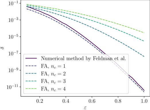
Figure 1: Evaluation of $\delta(\varepsilon)$ for general single and composite shuffle $(\varepsilon_{0},0)$-LDP mechanisms: for single composition protocols the numerical method by Feldman et al., (2021) is close to the tight bounds from FA ($n_{c}=1$). Their method is not directly applicable to compositions, for which the Fourier accountant also gives tight bounds. Number of users $n=10^{4}$ and the LDP parameter $\varepsilon_{0}=4.0$. To obtain the upper bounds using FA, we used parameter values $L=20$ and $m=10^{7}$.

3.4 Experimental comparison to the RDP bounds of Girgis et al., (2021)

Girgis et al., (2021) consider a protocol where only a randomly sampled, fixed sized subset of users send contributions to the shuffler on each round. This can be seen as a composition of a shuffler and a subsampling mechanism. We can generalise our analysis to the subsampled case via Proposition 30 of (Zhu et al.,, 2021), which states that if a pair of distributions $(P,Q)$ is a dominating pair of distributions for a mechanism $\mathcal{M}$ for datasets of size $\gamma n$ under $\sim$-neighbourhood relation (substitute relation), where $\gamma>0$ is the subsampling ratio (size of the subset divided by $n$), then $(\gamma\cdot P+(1-\gamma)\cdot Q,Q)$ is a dominating distribution for the subsampled mechanism $\mathcal{M}\circ S_{Subset}$, where the subsampling $S_{Subset}$ is carried out as described above. By Lemma 1 we know that the pair of distributions $(P,Q)$ of equation (3.1), where $C\sim\mathrm{Bin}(\gamma n-1,{\rm e}\hskip 1.0pt^{-\varepsilon_{0}})$ give a dominating pair of distributions for a general $\varepsilon_{0}$-LDP shuffler for datasets of size $\gamma n$, and therefore we can obtain $(\varepsilon,\delta)$-bounds for compositions of $\mathcal{M}\circ S_{Subset}$ using Corollary 3 and the pair of distributions $(\gamma\cdot P+(1-\gamma)\cdot Q,Q)$. As we see from Figure 2, the PLD-based approach gives considerably lower $\varepsilon(\delta)$-bounds. As $n_{c}$ increases, the FFT-based bound gets closer to the RDP bound, as noticed previously in (Koskela et al.,, 2020) in the case of subsampled Gaussian mechanism.

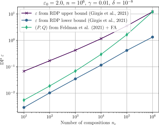
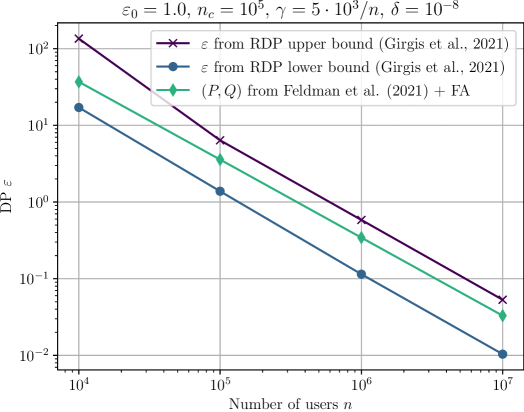
Figure 2: Evaluation of $\varepsilon(\delta)$ for compositions of subsampled shufflers. We compare the bounds obtained using FA and the PLD determined by the pair of distributions $(\gamma\cdot P+(1-\gamma)\cdot Q,Q)$ ($P$ and $Q$ from of equation (3.1) with $n$ replaced by $\gamma n$) and the RDP-bounds given in Thm. 2 of (Girgis et al.,, 2021) that are mapped to $\varepsilon(\delta)$-bounds using Lemma 1 of (Girgis et al.,, 2021). Above: bounds for different numbers of users $n$ when number of compositions $n_{c}$ is fixed. Below: number of compositions $n_{c}$ varies and $n$ is fixed. Here $\gamma$ denotes the subsampling ratio.

4 Shuffled $k$-randomised response

Balle et al., (2019) give a protocol for $n$ parties to compute a private histogram over the domain $[k]$ in the single-message shuffle model. The randomiser is parameterised by a probability $\gamma$, and consists of a $k$-ary randomised response mechanism ($k$-RR) that returns the true value with probability $1-\gamma$ and a uniformly random value with probability $\gamma$. Denote this $k$-RR randomiser by $\mathcal{R}_{\gamma,k,n}^{PH}$ and the shuffling operation by $\mathcal{S}$. Thus, we are studying the privacy of the shuffled randomiser $\mathcal{M}=\mathcal{S}\circ\mathcal{R}_{\gamma,k,n}^{PH}$.

Consider first the proof of Balle et al., (2019, Thm. 3.1). Assuming without loss of generality that the differing data element between $X$ and $X^{\prime}$, $X,X^{\prime}\in[k]^{n}$, is $x_{n}$, the (strong) adversary $A_{s}$ used by Balle et al., (2019, Thm. 3.1) is defined as follows:

Definition 1.

Let $\mathcal{M}=\mathcal{S}\circ\mathcal{R}_{\gamma,k,n}^{PH}$ be the shuffled $k$-RR mechanism, and w.l.o.g. let the differing element be $x_{n}$. We define adversary $A_{s}$ as an adversary with the view

$$\text{View}_{\mathcal{M}}^{A_{s}}(X)=\left((x_{1},\dots,x_{n-1}),\quad\beta\in\{0,1\}^{n},\quad(y_{\pi(1)},\dots,y_{\pi(n)})\right),$$

where $\beta$ is a binary vector identifying which parties answered randomly, and $\pi$ is a uniformly random permutation applied by the shuffler.

Assuming w.l.o.g. that the differing element $x_{n}=1$ and $x_{n}^{\prime}=2$, the proof then shows that for any possible view $V$ of the adversary $A_{s}$, $\tfrac{\mathbb{P}(\text{View}_{\mathcal{M}}^{A_{s}}(X)=V)}{\mathbb{P}(\text{View}_{\mathcal{M}}^{A_{s}}(X^{\prime})=V)}=\tfrac{n_{1}}{n_{2}}$, where $n_{i}$ denotes the number of messages received by the server with value $i$ after removing from the output $Y$ any truthful answers submitted by the first $n-1$ users. Moreover, Balle et al., (2019) show that for all neighbouring $X$ and $X^{\prime}$,

$$\text{View}_{\mathcal{M}}^{A_{s}}(X)\simeq_{(\varepsilon,\delta)}\text{View}_{\mathcal{M}}^{A_{s}}(X^{\prime})$$ (4.1)

for

$$\delta(\varepsilon)=\mathbb{P}\left(\frac{N_{1}}{N_{2}}\geq{\rm e}\hskip 1.0pt^{\varepsilon}\right),$$ (4.2)

where

$$N_{1}\sim\mathrm{Bin}\left(n-1,\frac{\gamma}{k}\right)+1,\quad N_{2}\sim\mathrm{Bin}\left(n-1,\frac{\gamma}{k}\right).$$ (4.3)

From the proof of Balle et al., (2019, Thm. 3.1) we directly get the following result for adaptive compositions of the $k$-RR shuffler.

Theorem 2.

Consider $n_{c}$ adaptive compositions of the $k$-RR shuffler mechanism $\mathcal{M}$ and an adversary $A_{s}$ as described in Def. 1 above. Then, the tight $(\varepsilon,\delta)$-bound is given by

$$\delta(\varepsilon)=\mathbb{P}\left(\sum\limits_{i=1}^{n_{c}}Z_{i}\geq\varepsilon\right),$$

where $Z_{i}$’s are independent and for all $1\leq i\leq n_{c}$, $Z_{i}\sim\log\left(\frac{N_{1}}{N_{2}}\right)$, where $N_{1}$ and $N_{2}$ are distributed as in (4.3).

Proof.

We first remark that in fact (4.2) holds when ${\rm e}\hskip 1.0pt^{\varepsilon}$ is replaced by any $\alpha\geq 0$, i.e., for any neighbouring $X$ and $X^{\prime}$, when $\alpha\geq 0$,

$$H_{\alpha}\big{(}\text{View}_{\mathcal{M}}^{A_{s}}(X)||\text{View}_{\mathcal{M}}^{A_{s}}(X^{\prime})\big{)}=\mathbb{P}\left(\frac{N_{1}}{N_{2}}\geq\alpha\right),$$ (4.4)

where $N_{1}\sim\mathrm{Bin}(n-1,\frac{\gamma}{k})+1$, $N_{2}\sim\mathrm{Bin}(n-1,\frac{\gamma}{k})$. This can be seen directly from the arguments of the proof of Balle et al., (2019, Thm. 3.1). Next, we may use a similar argument as in the proof of (Zhu et al.,, 2021, Thm. 10). By using (4.4) repeatedly, we see that for an adaptive composition of two mechanisms $\mathcal{M}_{1}$ and $\mathcal{M}_{2}$:

$$\delta(\varepsilon) =\mathbb{P}_{V\sim\text{View}_{\mathcal{M}_{1}}^{A_{s}}(X),V^{\prime}\sim\text{View}_{\mathcal{M}_{2}}^{A_{s}}(X,V)}\left[\frac{\mathbb{P}(\text{View}_{\mathcal{M}_{1}}^{A_{s}}(X)=V)\cdot\mathbb{P}(\text{View}_{\mathcal{M}_{2}}^{A_{s}}(X,V)=V^{\prime})}{\mathbb{P}(\text{View}_{\mathcal{M}_{1}}^{A_{s}}(X^{\prime})=V)\cdot\mathbb{P}(\text{View}_{\mathcal{M}_{2}}^{A_{s}}(X^{\prime},V)=V^{\prime})}\geq{\rm e}\hskip 1.0pt^{\varepsilon}\right]$$

$$=\mathbb{P}_{V\sim\text{View}_{\mathcal{M}_{1}}^{A_{s}}(X),V^{\prime}\sim\text{View}_{\mathcal{M}_{2}}^{A_{s}}(X,V)}\left[\frac{\mathbb{P}(\text{View}_{\mathcal{M}_{2}}^{A_{s}}(X,V)=V^{\prime})}{\mathbb{P}(\text{View}_{\mathcal{M}_{2}}^{A_{s}}(X^{\prime},V)=V^{\prime})}\geq{\rm e}\hskip 1.0pt^{\varepsilon-\log\frac{\mathbb{P}(\text{View}_{\mathcal{M}_{1}}^{A_{s}}(X)=V)}{\mathbb{P}(\text{View}_{\mathcal{M}_{1}}^{A_{s}}(X^{\prime})=V)}}\right]$$

$$=\mathbb{P}_{V\sim\text{View}_{\mathcal{M}_{1}}^{A_{s}}(X)}\left[\frac{N_{1}^{2}}{N_{2}^{2}}\geq{\rm e}\hskip 1.0pt^{\varepsilon-\log\frac{\mathbb{P}(\text{View}_{\mathcal{M}_{1}}^{A_{s}}(X)=V)}{\mathbb{P}(\text{View}_{\mathcal{M}_{1}}^{A_{s}}(X^{\prime})=V)}}\right]$$

$$=\mathbb{P}_{V\sim\text{View}_{\mathcal{M}_{1}}^{A_{s}}(X)}\left[\frac{\mathbb{P}(\text{View}_{\mathcal{M}_{1}}^{A_{s}}(X)=V)}{\mathbb{P}(\text{View}_{\mathcal{M}_{1}}^{A_{s}}(X^{\prime})=V)}\geq{\rm e}\hskip 1.0pt^{\varepsilon-\log\frac{N_{1}^{2}}{N_{2}^{2}}}\right]$$

$$=\mathbb{P}\left[\frac{N_{1}^{1}}{N_{2}^{1}}\geq{\rm e}\hskip 1.0pt^{\varepsilon-\log\frac{N_{1}^{2}}{N_{2}^{2}}}\right]$$

$$=\mathbb{P}\left[\frac{N_{1}^{1}\cdot N_{1}^{2}}{N_{2}^{1}\cdot N_{2}^{2}}\geq{\rm e}\hskip 1.0pt^{\varepsilon}\right]$$

$$=\mathbb{P}\left[\log\left(\frac{N_{1}^{1}}{N_{2}^{1}}\right)+\log\left(\frac{N_{1}^{2}}{N_{2}^{2}}\right)\geq\varepsilon\right],$$

where $N_{1}^{1},N_{1}^{2}\sim\mathrm{Bin}(n-1,\frac{\gamma}{k})+1$, $N_{2}^{1},N_{2}^{2}\sim\mathrm{Bin}(n-1,\frac{\gamma}{k})$. The proof for $n_{c}>2$ goes analogously.∎

Balle et al., (2019) showed that for adversary $A_{s}$ the shuffled mechanism $\mathcal{M}=\mathcal{S}\circ\mathcal{R}_{\gamma,k,n}^{PH}$ is $(\varepsilon,\delta)$-DP for any $k,n\in\mathbb{N}$, $\varepsilon\leq 1$ and $\delta\in(0,1]$ such that $\gamma=\max\left\{\tfrac{14\cdot k\cdot\log\left(2/\delta\right)}{(n-1)\cdot\varepsilon^{2}},\tfrac{27\cdot k}{(n-1)\cdot\varepsilon}\right\}.$ Comparison to this bound is shown in Figure 3.

4.1 Tight bounds for varying adversaries using Fourier accountant

Following the reasoning of the proof of Balle et al., (2019, Thm. 3.1), for adversary $A_{s}$ (see Def. 1), we can compute tight $\delta(\varepsilon)$-bounds using Thm. 2.

Having tight bounds also enables us to evaluate exactly how much different assumptions on the adversary cost us in terms of privacy. For example, instead of the adversary $A_{s}$ we can analyse a weaker adversary $A_{w}$, who has extra information only on the first $n-1$ parties. We formalise this as follows:

Definition 3.

Let $\mathcal{M}=\mathcal{S}\circ\mathcal{R}_{\gamma,k,n}^{PH}$ be the shuffled $k$-RR mechanism, and w.l.o.g. let the differing element be $x_{n}$. Adversary $A_{w}$ is an adversary with the view

$$\text{View}_{\mathcal{M}}^{A_{w}}(X)=\left((x_{1},\dots,x_{n-1}),\quad\beta\in\{0,1\}^{n-1},\quad(y_{\pi(1)},\dots,y_{\pi(n)})\right),$$

where $\beta$ is a binary vector identifying which of the first $n-1$ parties answered randomly, and $\pi$ is a uniformly random permutation applied by the shuffler.

Note that compared to the stronger adversary $A_{s}$ formalised in Def. 1 the difference is only in the vector $\beta$. We write $b=\sum_{i}\beta_{i}$, and $B$ for the corresponding random variable in the following.

The next theorem gives the random variables we need to calculate privacy bounds for adversary $A_{w}$:

Theorem 4.

Assume w.l.o.g. differing elements $x_{n}=1,x_{n}^{\prime}=2$, and adversary $A_{w}$ as given in Def. 3. To find a tight DP bound for $\mathcal{M}=\mathcal{S}\circ\mathcal{R}_{\gamma,k,n}^{PH}$ we can equivalently analyse the random variables $P_{w},Q_{w}$ defined as

$$P_{w}=P_{1}+P_{2},\quad Q_{w}=Q_{1}+Q_{2},$$ (4.5)

where

$$P_{1}\sim(1-\gamma)\cdot N_{1}|B,\quad P_{2}\sim\frac{\gamma}{k}\cdot(B+1),$$

$$Q_{1}\sim(1-\gamma)\cdot N_{2}|B,\quad Q_{2}\sim\frac{\gamma}{k}\cdot(B+1),$$

$$B\sim\mathrm{Bin}(n-1,\gamma),$$

$$N_{i}^{B}|B\sim\mathrm{Bin}(B,1/k),\quad i=1,\dots,k,$$

$$N_{1}|B=N_{1}^{B}|B+\mathrm{Bern}(1-\gamma+\gamma/k)$$

$$N_{2}|B=N_{2}^{B}|B+\mathrm{Bern}(\gamma/k).$$

As a direct corollary to this theorem, and analogously to Thm. 2, we have the following result which allows computing tight $\delta(\varepsilon)$-bounds against the adversary $A_{w}$ for adaptive compositions.

Theorem 5.

Consider $n_{c}$ adaptive compositions of the $k$-RR shuffler mechanism $\mathcal{M}$ and an adversary $A_{w}$ as described in Def. 3 above. Then, the tight $(\varepsilon,\delta)$-bound is given by

$$\delta(\varepsilon)=\mathbb{P}\left(\sum\limits_{i=1}^{n_{c}}Z_{i}\geq\varepsilon\right),$$

where $Z_{i}$’s are independent and for all $1\leq i\leq m$,

$$Z_{i}\sim\log\left(\frac{N_{1}}{N_{2}}\right),\quad N_{1}\sim P_{w},\quad N_{2}\sim Q_{w},$$

where $P_{w}$ and $Q_{w}$ are given in (4.5).

Proof.

See Thm. 2 proof. ∎

Figure 3 shows an empirical comparison of the tight bounds obtained with Fourier accountant assuming the stronger adversary $A_{s}$, which leads to the neighbouring random variables $P_{s},Q_{s}$ from (4.3), or the weaker adversary $A_{w}$, corresponding to $P_{w},Q_{w}$ from Thm. 4, together with the loose analytic bounds from Balle et al., (2019, Thm. 3.1). As shown in the Figure, tight bounds are considerably tighter than the analytic one. There is also a clear difference in the tight bounds resulting from assuming either the strong adversary $A_{s}$ or the weaker $A_{w}$. We remark that the evaluation of the distributions for $Z_{i}$’s in theorems 2 and 5 can be carried out in high accuracy in $\mathcal{O}(n)$-time using Hoeffding’s inequality similarly as in Lemma 3.2.

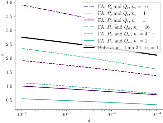
Figure 3: Shuffled $k$-randomised response: tight bounds are significantly better than the existing analytic one. Tight $(\varepsilon,\delta)$-DP bounds obtained using the Fourier accountant (FA) for different number of compositions $n_{c}$, and the loose analytical bound from Balle et al., (2019, Thm. 3.1) for a single composition. We apply FA to the $\delta(\varepsilon)$-expression of Thm. 2 ($P_{s}$ and $Q_{s}$), and to the $\delta(\varepsilon)$-expression of Thm. 5 ($P_{w}$ and $Q_{w}$). Both are tight bounds under the assumed adversary (stronger and weaker). FA with $P_{s},Q_{s}$ and $n_{c}=1$ is the tight bound with the same assumptions as used in the loose analytic bound. Total number of users $n=1000$, probability of randomising for each user $\gamma=0.25$, and $k=4$. For FA, we use parameter values $L=20$ and $m=10^{7}$.

5 On the difficulty of obtaining bounds in the general case

We have provided means to compute accurate $(\varepsilon,\delta)$-bounds for the general $\varepsilon_{0}$-LDP shuffler using the results by Feldman et al., (2021) and tight bounds for the case of $k$-randomised response. Using the following example, we illustrate the computational difficulty of obtaining tight bounds for arbitrary local randomisers. Consider neighbouring datasets $X,X^{\prime}\in\mathbb{R}^{n}$, where all elements of $X$ are equal, and $X^{\prime}$ contains one element differing by 1. Without loss of generality (due to shifting and scaling invariance of DP), we may consider the case where $X$ consists of zeros and $X^{\prime}$ has 1 at some element. Considering a mechanism $\mathcal{M}$ that consists of adding Gaussian noise with variance $\sigma^{2}$ to each element and then shuffling, we see that the adversary sees the output of $\mathcal{M}(X)$ distributed as

$$\mathcal{M}(X)\sim\mathcal{N}(0,\sigma^{2}I_{n}),$$

and the output $\mathcal{M}(X^{\prime})$ as the mixture distribution

$$\mathcal{M}(X^{\prime})\sim\tfrac{1}{n}\cdot\mathcal{N}(e_{1},\sigma^{2}I_{n})+\ldots+\tfrac{1}{n}\cdot\mathcal{N}(e_{n},\sigma^{2}I_{n}),$$

where $e_{i}$ denotes the $i$th unit vector. Determining the hockey-stick divergence $H_{{\rm e}\hskip 1.0pt^{\varepsilon}}(\mathcal{M}(X^{\prime})||\mathcal{M}(X))$ cannot be projected to a lower-dimensional problem, unlike in the case of the (subsampled) Gaussian mechanism, for example, which is equivalent to a one-dimensional problem Koskela and Honkela, (2021). This means that in order to obtain tight $(\varepsilon,\delta)$-bounds, we need to numerically evaluate the $n$-dimensional hockey-stick integral $H_{{\rm e}\hskip 1.0pt^{\varepsilon}}(\mathcal{M}(X^{\prime})||\mathcal{M}(X))$. Using a numerical grid as in FFT-based accountants is unthinkable due to the curse of the dimensionality. However, we may use the fact that for any data set $X$, the density function $f_{X}(t)$ of $\mathcal{M}(X)$ is a permutation-invariant function, meaning that for any $t\in\mathbb{R}^{n}$ and for any permutation $\sigma\in\pi_{n}$, $f_{X}\big{(}\sigma(t)\big{)}=f_{X}(t)$. This allows reduce the number of required points on a regular grid for the hockey stick integral from $O(m^{n})$ to $O(m^{n}/n!)$, where $m$ is the number of discretisation points in each dimension. Recent research on numerical integration of permutation-invariant functions (e.g. Nuyens et al.,, 2016) suggests it may be possible to significantly reduce or even eliminate the dependence on $n$ using more advanced integration techniques. In Figure 4 we have computed $H_{{\rm e}\hskip 1.0pt^{\varepsilon}}(\mathcal{M}(X^{\prime})||\mathcal{M}(X))$ up to $n=7$ using Monte Carlo integration on a hypercube $[-L,L]^{n}$ which requires $\approx 5\cdot 10^{7}$ samples for getting two correct significant figures for $n=7$.

Figure 4: Approximation of tight $\delta(\varepsilon)$ for shuffled outputs of Gaussian mechanisms ($\sigma=2.0$) by Monte Carlo integration of the hockey-stick divergence $H_{{\rm e}\hskip 1.0pt^{\varepsilon}}(\mathcal{M}(X^{\prime})||\mathcal{M}(X))$, using $5\cdot 10^{7}$ samples (two correct significant figures).

6 Discussion

We have shown how numerical privacy accounting can be used to calculate accurate upper bounds for compositions of various $(\varepsilon,\delta)$-DP mechanisms and different adversaries in the shuffle model. An alternative approach would be to use the Rényi differential privacy (Mironov,, 2017). However, as illustrated by the comparison against the results of Girgis et al., (2021) in Fig. 2, our numerical method leads to considerably tighter bounds. For shuffled mechanisms, the difference appears even more significant than for regular DP-SGD (Koskela et al.,, 2020, 2021), showing up to an order of magnitude reduction in $\varepsilon$.

Numerical and analytical privacy bounds are in many cases complementary and serve different purposes. Numerical accountants allow finding the tightest possible bounds for production and enable more unbiased comparison of algorithms when accuracy of accounting is not a factor. Analytical bounds enable theoretical research and understanding of scaling properties of algorithms, but the inaccuracy of the bounds raises the risk of misleading conclusions about privacy claims.

While our results provide significant improvements over previous state-of-the-art, they only provide optimal accounting for $k$-randomised response. Developing optimal accounting for more general mechanisms as well as extending the results to $(\varepsilon_{0},\delta_{0})$-LDP base mechanisms are important topics for future research.

Appendix A Auxiliary results for Section 3

In this section we give the needed expressions to determine the PLD

$$\omega_{P/Q}(s)=\sum\nolimits_{a,b}\mathbb{P}(P=(a,b))\cdot\delta_{s_{a,b}}(s),$$

where

$$s_{a,b}=\log\left(\frac{\mathbb{P}(P=(a,b))}{\mathbb{P}(Q=(a,b))}\right).$$

With these expressions, we can also determine the probability

$$\delta_{P/Q}(\infty) =\sum_{\{(a,b)\,:\,\mathbb{P}(Q=(a,b))=0)\}}\mathbb{P}(P=(a,b)).$$

Recall: denoting $q=\frac{{\rm e}\hskip 1.0pt^{\varepsilon_{0}}}{{\rm e}\hskip 1.0pt^{\varepsilon_{0}}+1}$, the distributions in (3.1) are given by the mixture distributions

$$P =q\cdot P_{1}+(1-q)\cdot P_{0},$$ (A.1)

$$Q =(1-q)\cdot P_{1}+q\cdot P_{0},$$

where

$$P_{1}=(A+1,C-A),\quad P_{0}=(A,C-A+1),$$

$$C\sim\mathrm{Bin}(n-1,{\rm e}\hskip 1.0pt^{-\varepsilon_{0}}),\quad A\sim\mathrm{Bin}(C,\tfrac{1}{2}).$$

A.1 Determining the log ratios $s_{a,b}$

To determine $s_{a,b}$’s, we need the following auxiliary results.

Lemma 1.

When $b>0$ and $a>0$, we have:

$$\mathbb{P}(P_{1}=(a,b))=\frac{a}{b}\cdot\mathbb{P}(P_{0}=(a,b)).$$

Proof.

We see that $P_{1}=(a,b)$ if and only if $A=a-1$ and $C=a+b-1$. Since

$$\mathbb{P}(A=a-1\,|\,C=a+b-1) ={a+b-1\choose a-1}\frac{1}{2^{a+b-1}}$$

$$=\frac{a}{b}\cdot{a+b-1\choose a}\frac{1}{2^{a+b-1}}$$

$$=\frac{a}{b}\cdot\mathbb{P}(A=a\,|\,C=a+b-1),$$

we see that

$$\mathbb{P}(P_{1}=(a,b)) =\mathbb{P}(C=a+b-1)\cdot\mathbb{P}(A=a-1\,|\,C=a+b-1)$$

$$=\mathbb{P}(C=a+b-1)\cdot\frac{a}{b}\cdot\mathbb{P}(A=a\,|\,C=a+b-1)$$

$$=\frac{a}{b}\cdot\mathbb{P}(P_{0}=(a,b)),$$

since $P_{0}=(a,b)$ if and only if $A=a$ and $C=a+b-1$. ∎

Using these expressions, and the fact that $\mathbb{P}(P_{0}=(a,0))=0$ for all $a$ and $\mathbb{P}(P_{1}=(0,b))=0$ for all $b$, we get the following expressions needed for $s_{a,b}$’s.

Lemma 2.

When $b>0$ and $a\geq 0$,

$$\frac{\mathbb{P}(P=(a,b))}{\mathbb{P}(Q=(a,b))}=\frac{q\cdot\frac{a}{b}+(1-q)}{q+(1-q)\frac{a}{b}}.$$

When $0<a\leq n$,

$$\frac{\mathbb{P}(P=(a,0))}{\mathbb{P}(Q=(a,0))}=\frac{q}{1-q}.$$

A.2 Probabilities $\mathbb{P}(P=(a,b))$

To determine $\omega_{P/Q}$, we still need to determine $\mathbb{P}(P=(a,b))$’s. These are given by the following expressions.

Lemma 3.

When $a>0$,

$$\mathbb{P}(P_{1}=(a,b))={n-1\choose i}{i\choose j}p^{i}(1-p)^{n-1-i}\frac{1}{2^{i}},$$

where $(a,b)=(j+1,i-j)$ (i.e., $C=i$ and $A=j$), and

$$\mathbb{P}(P_{0}=(a,b))=\frac{{\rm e}\hskip 1.0pt^{-\varepsilon_{0}}}{1-{\rm e}\hskip 1.0pt^{-\varepsilon_{0}}}\frac{n-a-b}{2a}\mathbb{P}(P_{1}=(a,b)).$$

For $0<b\leq n$,

$$\mathbb{P}(P_{1}=(0,b))=0$$

and

$$\mathbb{P}(P_{0}=(0,b))={n-1\choose b-1}\left(\frac{{\rm e}\hskip 1.0pt^{-\varepsilon_{0}}}{2}\right)^{b-1}(1-{\rm e}\hskip 1.0pt^{-\varepsilon_{0}})^{n-b}.$$

Proof.

The expressions follow directly from the definitions of $P_{0}$, $P_{1}$, $A$ and $C$. ∎

Appendix B More detailed derivation of the probabilities for $k$-ary RR

Recall from Section 5.1 of the main text: we consider the case where the adversary sees a vector $\beta$ of length $n-1$ identifying clients who submit only noise, except for the client with the differing element, and write $b=\sum_{i}\beta_{i}$. The adversary can remove all truthfully reported values by the clients $[n-1]$. Denote the observed counts after removal by $n_{i},i=1,\dots,k$, so $\sum_{i=1}^{k}n_{i}=b+1$, and write $\mathcal{R}$ for the local randomiser. We now have

$$\mathbb{P}(\text{View}_{\mathcal{M}}^{A_{w}}(\mathbf{x})=V) =\sum_{i=1}^{k}\mathbb{P}(N_{1}=n_{1},\dots,N_{i}=n_{i}-1,N_{i+1}=n_{i+1},\ldots$$

$$N_{k}=n_{k}|B)\cdot\mathbb{P}(\mathcal{R}(x_{n})=i)\cdot\mathbb{P}(B=b)$$

$$=\binom{b}{n_{1}-1,n_{2},\dots,n_{k}}\left(\frac{1}{k}\right)^{b}\cdot\left(1-\gamma+\frac{\gamma}{k}\right)\cdot\gamma^{b}(1-\gamma)^{n-1-b}$$

$$+\sum_{i=2}^{k}\binom{b}{n_{1},\dots,n_{i}-1,n_{i+1},\dots,n_{k}}\left(\frac{1}{k}\right)^{b}\cdot\frac{\gamma}{k}\cdot\gamma^{b}(1-\gamma)^{n-1-b}$$

$$=\binom{b}{n_{1},n_{2},\dots,n_{k}}\frac{\gamma^{b}(1-\gamma)^{n-1-b}}{k^{b}}\left[n_{1}(1-\gamma+\frac{\gamma}{k})+\sum_{i=2}^{k}n_{i}\frac{\gamma}{k}\right]$$

$$=\binom{b}{n_{1},n_{2},\dots,n_{k}}\frac{\gamma^{b}(1-\gamma)^{n-1-b}}{k^{b}}\cdot$$

$$\quad\quad\quad\left[n_{1}(1-\gamma+\frac{\gamma}{k})+(b+1-n_{1})\frac{\gamma}{k}\right]$$

$$=\binom{b}{n_{1},n_{2},\dots,n_{k}}\frac{\gamma^{b}(1-\gamma)^{n-1-b}}{k^{b}}\left[n_{1}(1-\gamma)+\frac{\gamma}{k}(b+1)\right].$$

Noting that $\mathbb{P}(\mathcal{R}(x_{n}^{\prime})=i)=(1-\gamma+\frac{\gamma}{k})$ when $i=2$ and $\frac{\gamma}{k}$ otherwise, repeating essentially the above steps gives

$$\mathbb{P}(\text{View}_{\mathcal{M}}^{A_{w}}(\mathbf{x}^{\prime})=V) =\sum_{i=1}^{k}\mathbb{P}(N_{1}=n_{1},\dots,N_{i}=n_{i}-1,N_{i+1}=n_{i+1},\ldots,$$

$$\quad N_{k}=n_{k}|B)\cdot\mathbb{P}(\mathcal{R}(x_{n}^{\prime})=i)\cdot\mathbb{P}(B=b)$$

$$=\binom{b}{n_{1},n_{2},\dots,n_{k}}\frac{\gamma^{b}(1-\gamma)^{n-1-b}}{k^{b}}\left[n_{2}(1-\gamma)+\frac{\gamma}{k}(b+1)\right].$$

B.1 Proof of Theorem 4

The next theorem gives the random variables we need to calculate privacy bounds for the weaker adversary $A_{w}$:

Theorem 1.

Assume w.l.o.g. differing elements $x_{n}=1,x_{n}^{\prime}=2$, and adversary $A_{w}$ as given in Def. 3. To find a tight DP bound for $\mathcal{M}=\mathcal{S}\circ\mathcal{R}_{\gamma,k,n}^{PH}$ we can equivalently analyse the random variables $P_{w},Q_{w}$ defined as

$$P_{w}=P_{1}+P_{2},\quad Q_{w}=Q_{1}+Q_{2},$$ (B.1)

where

$$P_{1}\sim(1-\gamma)\cdot N_{1}|B,\quad P_{2}\sim\frac{\gamma}{k}\cdot(B+1),$$

$$Q_{1}\sim(1-\gamma)\cdot N_{2}|B,\quad Q_{2}\sim\frac{\gamma}{k}\cdot(B+1),$$

$$B\sim\mathrm{Bin}(n-1,\gamma),$$

$$N_{i}^{B}|B\sim\mathrm{Bin}(B,1/k),\quad i=1,\dots,k,$$

$$N_{1}|B=N_{1}^{B}|B+\mathrm{Bern}(1-\gamma+\gamma/k)$$

$$N_{2}|B=N_{2}^{B}|B+\mathrm{Bern}(\gamma/k).$$

Proof.

Notice that for $k$-RR, seeing the shuffler output is equivalent to seeing the total counts for each class resulting from applying the local randomisers to $X$ or $X^{\prime}$. The adversary $A_{w}$ can remove all truthfully reported values by client $j$, $j\in[n-1]$. Denote the observed counts after this removal by $n_{i},i=1,\dots,k$, so $\sum_{i=1}^{k}n_{i}=b+1$. We now have

$$\mathbb{P}(\text{View}_{\mathcal{M}}^{A_{w}}(X)=V) =\sum_{i=1}^{k}\mathbb{P}(N_{1}=n_{1},\dots,N_{i}=n_{i}-1,\dots,N_{k}=n_{k}|b)\cdot\mathbb{P}(\mathcal{R}_{\gamma,k,n}^{PH}(x_{n})=i)\cdot\mathbb{P}(B=b)$$

$$=\binom{b}{n_{1},n_{2},\dots,n_{k}}\frac{\gamma^{b}(1-\gamma)^{n-1-b}}{k^{b}}\left[n_{1}(1-\gamma)+\frac{\gamma}{k}(b+1)\right],$$

where the second equation comes from the fact that the random values in $k$-RR follow a Multinomial distribution. Noting then that $\mathbb{P}(\mathcal{R}_{\gamma,k,n}^{PH}(x_{n}^{\prime})=i)=(1-\gamma+\frac{\gamma}{k})$ when $i=2$ and $\frac{\gamma}{k}$ otherwise, repeating essentially the same steps gives

$$\mathbb{P}(\text{View}_{\mathcal{M}}^{A_{w}}(X^{\prime})=V)=\binom{b}{n_{1},n_{2},\dots,n_{k}}\frac{\gamma^{b}(1-\gamma)^{n-1-b}}{k^{b}}\left[n_{2}(1-\gamma)+\frac{\gamma}{k}(b+1)\right].$$

Looking at ratio of the two final probabilities we have

$$\mathbb{P}_{V\sim\text{View}_{\mathcal{M}}^{A_{w}}(X)}\left[\frac{\mathbb{P}(\text{View}_{\mathcal{M}}^{A_{w}}(X)=V)}{\mathbb{P}(\text{View}_{\mathcal{M}}^{A_{w}}(X^{\prime})=V)}\geq e^{\varepsilon}\right]=\mathbb{P}\left[\frac{N_{1}|B\cdot(1-\gamma)+\frac{\gamma}{k}(B+1)}{N_{2}|B\cdot(1-\gamma)+\frac{\gamma}{k}(B+1)}\geq e^{\varepsilon}\right],$$

where we write $N_{i}|B,i\in\{1,2\}$ for the random variable $N_{i}$ conditional on $B$. This shows that for DP bounds, the adversaries’ full view is equivalent to only considering the joint distribution of $N_{i},B,i\in\{1,2\}$, and we can therefore look at the neighbouring random variables

$$P_{w}=P_{1}+P_{2},\quad Q_{w}=Q_{1}+Q_{2},$$ (B.2)

where

$$P_{1}\sim(1-\gamma)\cdot N_{1}|B,\quad P_{2}\sim\frac{\gamma}{k}\cdot(B+1),$$

$$Q_{1}\sim(1-\gamma)\cdot N_{2}|B,\quad Q_{2}\sim\frac{\gamma}{k}\cdot(B+1).$$

Writing $n_{i}^{B}$ for the count in class $i$ resulting from the noise sent by the $n-1$ parties, from $k$-RR definition we also have

$$B\sim\mathrm{Bin}(n-1,\gamma)\quad\text{ and }\quad N_{i}^{B}|B\sim\mathrm{Bin}(B,1/k),$$ (B.3)

$i=1,\ldots,k.$ As $V\sim\text{View}_{\mathcal{M}}^{A_{w}}(X)$, we finally have

$$N_{1}|B=N_{1}^{B}|B+\mathrm{Bern}(1-\gamma+\gamma/k)$$ (B.4)

$$N_{2}|B=N_{2}^{B}|B+\mathrm{Bern}(\gamma/k).$$

The distributions (B.3) and (B.4) determine the neighbouring distributions $P_{w}$ and $Q_{w}$ given in (B.2) which completes the proof. ∎

The proof of the following result which allows computing tight $\delta(\varepsilon)$-bounds against the adversary $A_{w}$ for adaptive compositions, goes analogously to the proof of Thm. 1.

Theorem 2.

Consider $m$ compositions of the $k$-RR shuffler mechanism $\mathcal{M}$ and an adversary $A_{w}$. Then, the tight $(\varepsilon,\delta)$-bound is given by

$$\delta(\varepsilon)=\mathbb{P}\left(\sum\limits_{i=1}^{m}Z_{i}\geq\varepsilon\right),$$

where $Z_{i}$’s are independent and for all $1\leq i\leq m$,

$$Z_{i}\sim\log\left(\frac{N_{1}}{N_{2}}\right),\quad N_{1}\sim P_{w},\quad N_{2}\sim Q_{w},$$

where $P_{w}$ and $Q_{w}$ are given in (4.5).

References

• Balle et al., (2019) Balle, B., Bell, J., Gascón, A., and Nissim, K. (2019). The privacy blanket of the shuffle model. In Annual International Cryptology Conference, pages 638–667. Springer.
• Balle et al., (2020) Balle, B., Bell, J., Gascón, A., and Nissim, K. (2020). Private summation in the multi-message shuffle model. In Proceedings of the 2020 ACM SIGSAC Conference on Computer and Communications Security, pages 657–676.
• Bittau et al., (2017) Bittau, A., Erlingsson, Ú., Maniatis, P., Mironov, I., Raghunathan, A., Lie, D., Rudominer, M., Kode, U., Tinnes, J., and Seefeld, B. (2017). Prochlo: Strong privacy for analytics in the crowd. In Proceedings of the 26th Symposium on Operating Systems Principles, pages 441–459.
• Cheu et al., (2019) Cheu, A., Smith, A., Ullman, J., Zeber, D., and Zhilyaev, M. (2019). Distributed differential privacy via shuffling. In Annual International Conference on the Theory and Applications of Cryptographic Techniques, pages 375–403. Springer.
• Dwork et al., (2006) Dwork, C., McSherry, F., Nissim, K., and Smith, A. (2006). Calibrating noise to sensitivity in private data analysis. In Proc. TCC 2006, pages 265–284.
• Dwork and Roth, (2014) Dwork, C. and Roth, A. (2014). The algorithmic foundations of differential privacy. Found. Trends Theor. Comput. Sci., 9(3–4):211–407.
• Erlingsson et al., (2019) Erlingsson, Ú., Feldman, V., Mironov, I., Raghunathan, A., Talwar, K., and Thakurta, A. (2019). Amplification by shuffling: From local to central differential privacy via anonymity. In Proceedings of the Thirtieth Annual ACM-SIAM Symposium on Discrete Algorithms, pages 2468–2479. SIAM.
• Feldman et al., (2021) Feldman, V., McMillan, A., and Talwar, K. (2021). Hiding among the clones: A simple and nearly optimal analysis of privacy amplification by shuffling. In 2021 IEEE 62nd Annual Symposium on Foundations of Computer Science. IEEE.
• Ghazi et al., (2021) Ghazi, B., Golowich, N., Kumar, R., Pagh, R., and Velingker, A. (2021). On the power of multiple anonymous messages: Frequency estimation and selection in the shuffle model of differential privacy. In Canteaut, A. and Standaert, F.-X., editors, Advances in Cryptology – EUROCRYPT 2021, pages 463–488, Cham. Springer International Publishing.
• Girgis et al., (2021) Girgis, A., Data, D., Diggavi, S., Kairouz, P., and Suresh, A. T. (2021). Shuffled model of differential privacy in federated learning. In International Conference on Artificial Intelligence and Statistics, pages 2521–2529. PMLR.
• Gopi et al., (2021) Gopi, S., Lee, Y. T., and Wutschitz, L. (2021). Numerical composition of differential privacy. In Advances in Neural Information Processing Systems.
• Kasiviswanathan et al., (2011) Kasiviswanathan, S. P., Lee, H. K., Nissim, K., Raskhodnikova, S., and Smith, A. (2011). What can we learn privately? SIAM Journal on Computing, 40(3):793–826.
• Koskela and Honkela, (2021) Koskela, A. and Honkela, A. (2021). Computing differential privacy guarantees for heterogeneous compositions using fft. arXiv preprint arXiv:2102.12412.
• Koskela et al., (2020) Koskela, A., Jälkö, J., and Honkela, A. (2020). Computing tight differential privacy guarantees using FFT. In International Conference on Artificial Intelligence and Statistics, pages 2560–2569. PMLR.
• Koskela et al., (2021) Koskela, A., Jälkö, J., Prediger, L., and Honkela, A. (2021). Tight differential privacy for discrete-valued mechanisms and for the subsampled gaussian mechanism using FFT. In International Conference on Artificial Intelligence and Statistics, pages 3358–3366. PMLR.
• Mironov, (2017) Mironov, I. (2017). Rényi differential privacy. In 2017 IEEE 30th Computer Security Foundations Symposium (CSF), pages 263–275.
• Nuyens et al., (2016) Nuyens, D., Suryanarayana, G., and Weimar, M. (2016). Rank-1 lattice rules for multivariate integration in spaces of permutation-invariant functions - error bounds and tractability. Adv. Comput. Math., 42(1):55–84.
• Sommer et al., (2019) Sommer, D. M., Meiser, S., and Mohammadi, E. (2019). Privacy loss classes: The central limit theorem in differential privacy. Proceedings on Privacy Enhancing Technologies, 2019(2):245–269.
• Zhu et al., (2021) Zhu, Y., Dong, J., and Wang, Y.-X. (2021). Optimal accounting of differential privacy via characteristic function. arXiv preprint arXiv:2106.08567.