Fractal generation in a two-dimensional active-nematic fluid

Abstract

Active fluids, composed of individual self-propelled agents, can generate complex large-scale coherent flows. A particularly important laboratory realization of such an active fluid is a system composed of microtubules, aligned in a quasi-two-dimensional (2D) nematic phase, and driven by ATP-fueled kinesin motor proteins. This system exhibits robust chaotic advection and gives rise to a pronounced fractal structure in the nematic contours. We characterize such experimentally derived fractals using the power spectrum and discover that the power spectrum decays as $k^{-\beta}$ for large wavenumbers $k$. The parameter $\beta$ is measured for several experimental realizations. Though $\beta$ is effectively constant in time, it does vary with experimental parameters, indicating differences in the scale-free behavior of the microtubule-based active nematic. Though the fractal patterns generated in this active system are reminiscent of passively advected dye in 2D chaotic flows, the underlying mechanism for fractal generation is more subtle. We provide a simple, physically inspired mathematical model of fractal generation in this system that relies on the material being locally compressible, though the total area of the material is conserved globally. The model also requires that large-scale density variations be injected into the material periodically. The model reproduces the power spectrum decay $k^{-\beta}$ seen in experiments. Linearizing the model of fractal generation about the equilibrium density, we derive an analytic relationship between $\beta$ and a single dimensionless quantity $r$, which characterizes the compressibility.

Active fluids are out-of-equilibrium systems that exhibit spontaneous flow dynamics as they consume energy locally to generate material stresses Marchetti et al. (2013). There are many fascinating examples of active fluids in nature that cross a wide range of length scales, from bacterial colonies Dell’Arciprete et al. (2018); You et al. (2018); Li et al. (2019) and cellular sheets Saw et al. (2017); Kawaguchi, Kageyama, and Sano (2017) to bird flocks Toner and Tu (1995) and insect swarms Buhl et al. (2006). We study a laboratory model of an active fluid with nematic ordering Sanchez et al. (2012), which is manifested by a striped pattern whose orientation varies throughout the fluid. This system exhibits spontaneous chaotic advection on submilimeter scales, thus making it an interesting paradigm for studies of chaotic dynamics. We show that the density fluctuations inherent in the striped patterning exhibit a fractal scaling. We then provide a simplified mathematical model for the generation of this fractal structure. This model shows how the material properties can be quantitatively linked to the decay of the power spectrum on small scales. We believe this provides an interesting new model of fractal generation in addition to providing insight into the physics of active nematics.

I Introduction

We examine a quasi-two-dimensional (2D) synthetic active nematic fluid, composed of biologically derived subunits Ndlec et al. (1997), in which the rod-like microtubule subunits are driven relative to each other by the action of kinesin motor proteins. In recent years, this system has become an important prototype for active fluids, with numerous experimental and theoretical studies Sanchez et al. (2012); Henkin et al. (2014); Giomi (2015); DeCamp et al. (2015); Guillamat, Ignés-Mullol, and Sagués (2016); Doostmohammadi et al. (2017); Guillamat, Ignés-Mullol, and Sagués (2017); Shendruk et al. (2017); Lemma et al. (2019); Tan et al. (2019). A key characteristic of this fluid is the emergence of mobile topological defects; points where the orientational order of the nematic phase breaks down. Positive and negative defects occur spontaneously as a result of the active flows, separate from each other and ultimately annihilate with other defects of their opposite charge in the fluid. In recent work, our group analyzed the motion of these defects in the context of chaotic mixing Tan et al. (2019), revealing that the defects can be treated as virtual stirring rods, which braid around each other, driving advective flows that stretch and fold the material.

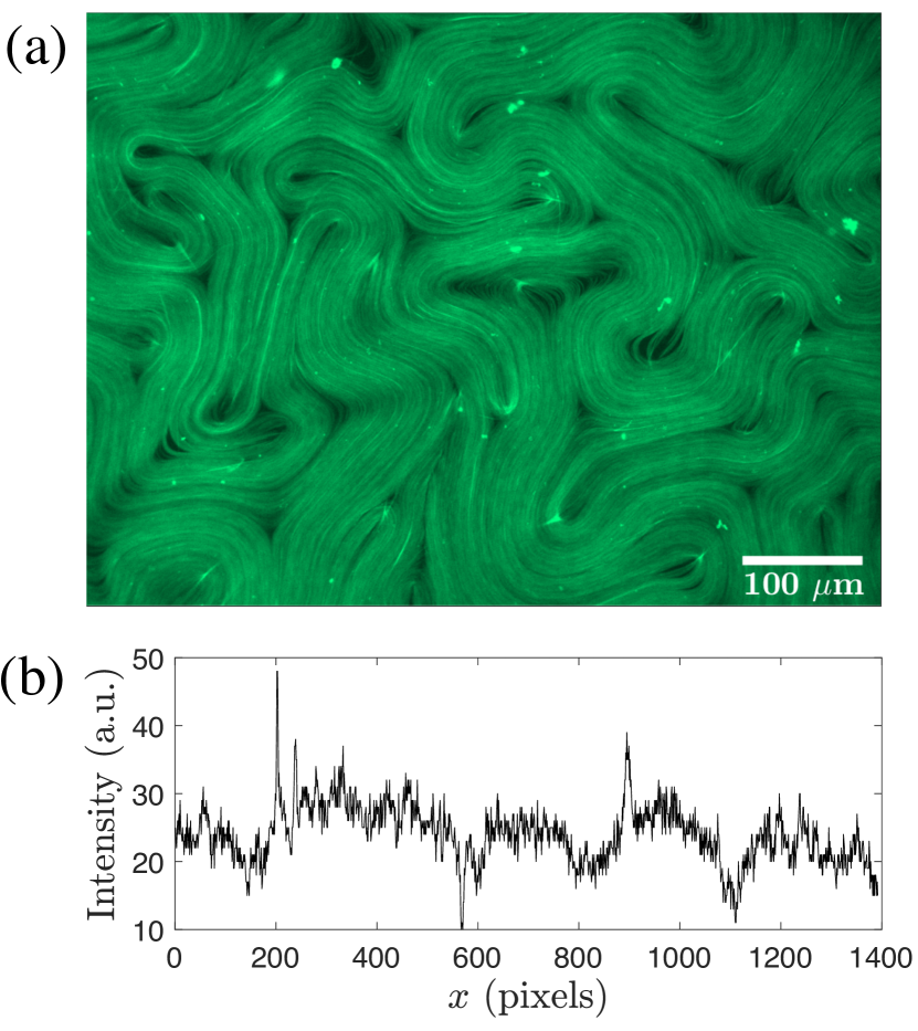
One of the most striking features of 2D microtubule-based active nematics is the visually distinctive patterns of folded dark and light bands of varying intensity (Fig. 1a). These folded patterns appear fractal, with finer structure apparent at smaller length scales. These fractal patterns are the subject of the current paper. The fractal analysis of images has a rich history across numerous disciplines, with many quantitative measures of fractal behavior introduced and utilized Peitgen and Saupe (1988); Soille and Rivest (1996); Lopes and Betrouni (2009); Bies et al. (2016); Nayak, Mishra, and Palai (2019). Fractal dimension is a well known tool and various definitions are commonly used. Here we choose to investigate the closely related decay of the power spectrum at large wavenumbers, i.e. small length scales. We analyze experimental images of active nematics, using data sets first reported in Ref. Tan et al., 2019. We find that power, i.e. the norm-squared of the Fourier coefficients, scales as a power-law $k^{-\beta}$ in the wavenumber $k$. This power-law behavior begins at the active length scale of the system, roughly the spacing between topological defects, and continues down to smaller scales, eventually being dominated by pixel noise. In a log-log plot, power versus $k$ displays a strikingly linear behavior over a wide range of $k$ values, from which we extract $\beta$. The value of $\beta$ is roughly constant in time.

Fractal patterns are well known to occur within the passive advection of material in a traditional 2D fluid Tel et al. (2005); Aguirre, Viana, and Sanjuán (2009); Lai and Tél (2010); Aref et al. (1989); Muzzio et al. (1992); Péntek et al. (1995). This is evident on large planetary scales, e.g. plankton blooms in the ocean Tel et al. (2005); Sandulescu et al. (2007), or on small laboratory scales, e.g. microfluidic devices Truesdell et al. (2003); Phelan, Hughes, and Pathak (2008). However, in a confined, incompressible flow, such fractal behavior is transient; eventually the system becomes well mixed and the fractal pattern washes out Muzzio et al. (1992). Persistent fractal behavior can arise in an open incompressible flow, when a constant stream of impurity enters and then exits a chaotic mixing region. However, the fractal structure witnessed in the active microtubule-based nematic is both persistent and confined. Furthermore, the microtubule system is also incompressible, or area-preserving, at least when averaged over a large enough domain. On smaller length scales, laboratory videos do show local compression of microtubule bundles and the creation and expansion of small voids. (See the online supplemental video.) Despite this, most continuum-based simulations assume local incompressibility from the start Giomi (2015); Doostmohammadi et al. (2017); Shendruk et al. (2017).

Figure 1: a) A fluorescence microscopy image of the microtubule system. b) The intensity across the top row of panel a.

We present a simple model for the creation of fractal structure that does not assume incompressibility on small length scales. Area is, however, preserved at the active length scale. Similarly, density is not constant; the patterns seen in the active nematic are, after all, due to local variations in density. Our model contains three distinct steps: 1) extension of the material in the direction of the director field, i.e. along the microtubule bundles, and compression in the perpendicular direction; 2) folding of the material back over itself in a horseshoe pattern; and 3) creation of new large-scale density fluctuations at the active length scale. A critical aspect of this model is that the compressibility in Step 1 varies with density. We find that this simple model generates $k^{-\beta}$ scaling in the power spectrum with a well defined $\beta$ value.

To better understand the model’s consequences, we conduct an analysis of the fractal formation to first order in the density fluctuations. Within this linear analysis, we analytically compute $\beta$ and find that it depends solely on a dimensionless parameter $r$, that characterizes the compressibility. The fractal behavior is lost if the system is incompressible.

This model is not intended to be a quantitatively faithful simulation of all the physics of a microtubule-based active nematic. Rather it is a reduced model designed to highlight the key physical processes necessary to create fractal structure. The lessons learned here could be incorporated into more quantitatively accurate numerical simulations in the future.

Note that our work should be distinguished from prior studies of scale-free behavior in active nematics Giomi (2015); Alert, Joanny, and Casademunt (2020). These studies assume uniform density, so are not sensitive to the density fluctuations considered here. Instead, they consider the decay in the energy and enstrophy spectra, which have a universal power-law behavior at small scales.

This paper is organized as follows. Section II presents our results on the spectral decay of experimental images of the active nematic material. Section III explains our three-step model of fractal generation. Section IV linearizes the model in the density fluctuations. Section V discusses the special case in which Step 1 of our model is incompressible but Step 3 is not. Conclusions are in Sect. VI.

II Experimentally measured power-spectrum decay of microtubule-based active nematics

The analysis here is based on the experimental data presented in Ref. Tan et al., 2019, where a complete description of the experimental technique is given. In brief, a quasi-2D layer of microtubules is suspended at an oil-water boundary. The microtubules are at high density and form bundles due to the use of a depletion agent (polyethylene glycol). Kinesin molecular motors, joined together in clusters, serve to cross-link the microtubules. ATP is added to the solution to power the molecular motors, which walk along the microtubules from their negative end to their positive end. Neighboring microtubules of opposite polarity are pushed in opposing directions by the motor clusters to produce the active stress in the material. This local stress produces large-scale dynamics in the 2D microtubule layer. The system is imaged using fluorescence microscopy. See Fig. 1a and the online supplemental video. Experiments were performed with six different ATP concentrations. The higher the ATP concentration, the more activity is induced in the system and the faster the system evolves, assuming all other factors are held constant.

Figure 2: a) Power spectrum (black) of Fig. 1b. The blue curve is the power spectrum averaged in $\log k$ space using a Gaussian of width $\sigma=0.4$. (See Appendix.) The red line is a linear fit to this average. The vertical dashed line denotes the $k$ value corresponding to the velocity autocorrelation length. Note that the scaling is chosen so that $k=L_{0}/\lambda$ for wavelength $\lambda$, where $L_{0}$ is the width of the image; b) The 1D power spectrum averaged over all rows of the image in Fig. 1a; c) The angle-averaged 2D power spectrum of the image in Fig. 1a; d) The 1D (black) and 2D (green) $\beta$ values as a function of time. The red curve is the green curve shifted down by 1. All data in these figures were taken at an ATP concentration of $50\mu$M.

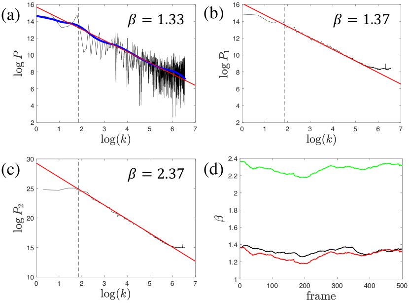
We analyse the power spectrum of the resulting experimental images $f(x,y)$ in two ways. In the first technique, we compute the 1D Fourier transform $\tilde{f}(k_{x};y)$ of each row; here $y$ labels the row and $k_{x}$ is the $x$ wave vector. The power spectrum of row $y$ is then the norm-squared of the Fourier coefficients versus $k=|k_{x}|$, i.e. $P(k;y)=|\tilde{f}(k;y)|^{2}$. For example, Fig. 1b shows the intensity of the top row in Fig. 1a; Fig. 2a shows a log-log plot of the resulting power spectrum (black). To better see the spectral decay, we smooth the power spectrum in $\log k$ as discussed in the Appendix. This average is shown as the smooth blue curve. Finally, the blue curve is fit to a linear decay, shown in red, with slope $-1.33$. The vertical dashed line marks the value $k=L_{0}/\ell$, where $L_{0}$ is the width of the image and $\ell$ is the active length scale, defined here as the velocity autocorrelation length Lemma et al. (2019); Hemingway et al. (2016) of the active nematic, computed in Ref. Tan et al., 2019. Note that the linear fall off begins at $k$ values larger than approximately $L_{0}/\ell$.

The initial (black) power spectrum in Fig. 2a has large fluctuations, which we can reduce by averaging $P(k;y)$ over all the rows $y$ of the image, producing the averaged 1D power spectrum $P_{1}(k)$. This is shown as the black power spectrum in Fig. 2b, where the fluctuations have diminished dramatically. The red fit line is obtained as in Fig. 2a, i.e. the power spectrum is first smoothed in $\log k$ (not shown in Fig. 2b), and then the red line is fit to this average. The resulting slope is $-1.37$, comparable to that of Fig. 2a.

The second technique for computing the spectral decay is to first take the 2D Fourier transform $\tilde{f}(k_{x},k_{y})$ of the entire image (in practice, a square subset of the image). Then $P(k_{x},k_{y})=|\tilde{f}(k_{x},k_{y})|^{2}$ is averaged over angle to produce the 2D power spectrum

$$P_{2}(k)=\frac{1}{2\pi}\int_{0}^{2\pi}P(k\cos(\phi),k\sin(\phi))\,d\phi,$$ (1)

which is shown in Fig. 2c. Its fluctuations are roughly comparable to that of averaging over the rows (Fig. 2b). The data is again smoothed in $\log k$ and subsequently fit to the red line, with slope $-2.37$.

Note that these power spectra show that there is a single active length scale, which can be defined as the velocity autocorrelation length $\ell$, as done here. This is consistent with what is known from prior publications, e.g. Ref. Lemma et al., 2019. On scales smaller than the active length scale, the density distribution appears scale free.

Figure 3: The $\beta$ value averaged over all 500 frames of the active nematic video for experiments performed at six different ATP concentrations: 50, 75, 100, 250, 500, 1000 $\mu$M. The black data is computed from $P_{1}$ and the red data from $P_{2}$, shifted down by 1. Error bars are the standard deviations of $\beta$ over all frames.

We now investigate the time-dependence of the $\beta$’s. Figure 2d shows $\beta$ computed from $P_{1}$ (black) and $P_{2}$ (green) for each of 500 experimental frames. There is modest variation in each graph. Note that the two curves differ by about 1. This is made clearer by the red curve in Fig. 2d, which is the green curve shifted down by 1. The reason for this correspondence can be understood as follows. Suppose the original image $f(x,y)$ were independent of $y$, consisting only of vertical stripes. Then $\tilde{f}(k_{x},k_{y})$ could be written as $\tilde{f}(k_{x};y)\delta_{k_{y}0}$, i.e. the 2D Fourier transform depends on $k_{x}$ just as the 1D Fourier transform of any (equivalent) row of the image and is nonzero only when $k_{y}=0$, since the image is constant in $y$. If $P(k_{x};y)$ falls off like $k^{-\beta}$, then the angular average of $P(k_{x},k_{y})$ is one factor of $k$ smaller due to dividing by the circumference $2\pi k$. The close agreement between the red and black curves confirms the validity of our analysis.

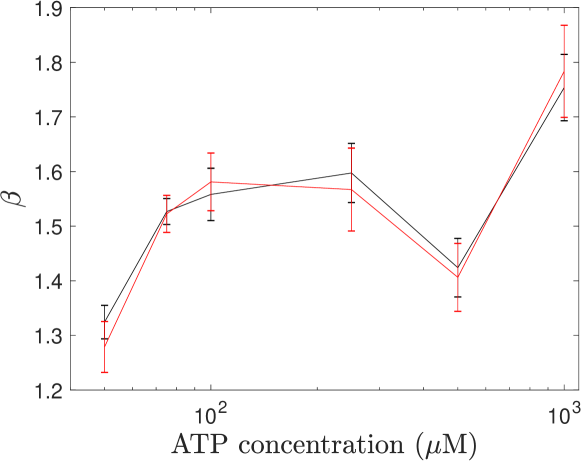
Separate experiments were run for six different ATP concentrations. Figure 3 shows the $\beta$ value averaged over all 500 frames for each ATP concentration. The black data is computed from $P_{1}$ and the red data from $P_{2}$, shifted down by one. Error bars are the standard deviation of $\beta$ over the 500 frames. Note that the $P_{1}$ and $P_{2}$ data are consistent across all six experimental runs. However, there are significant variations in $\beta$ from one experiment to the next, indicating that the nature of the scale-free behavior is not universal.

III Model of fractal generation

III.1 Step 1: One-dimensional model of compression dynamics

We consider a model of the material in which the microtubule bundles, and hence the directors, point along the $y$ direction everywhere, and in which the density $\rho$ depends solely on $x$. See Fig. 4a. We assume that this material is under a constant stress perpendicular to the directors and that the response of the material depends solely on the density $\rho(x)$. Specifically, the relative change in length $dL/L$ of any interval $[x_{0},x_{1}]$, where $L=x_{1}-x_{0}$, over time $dt$ depends solely on the average density $\bar{\rho}$ of the interval, i.e.

$$\frac{dL}{dt} =g(\bar{\rho})L,$$ (2)

$$\bar{\rho} =\frac{1}{L}\int_{x_{0}}^{x_{1}}\rho(x)dx,$$ (3)

where $g$ is the compression rate for a given average density. The assumption that Eq. (2) applies to all intervals is equivalent to $g$ being an affine function, which we write as

$$g(\bar{\rho})=-\alpha(1-\bar{\rho}/\rho_{m}),$$ (4)

where $\alpha$ and $\rho_{m}$ are constants. We take $\rho_{m}>0$ and $\alpha>0$, so that the material becomes less compressible at higher density, becoming incompressible for the given stress when the average density is $\rho_{m}$. Using $v(x,t)$ for the velocity of the material at position $x$ and time $t$, Eqs. (2)–(4) imply

$$\frac{1}{L}\int_{x_{0}}^{x_{1}}\frac{\partial v}{\partial x}dx =\frac{1}{L}[v(x_{1})-v(x_{0})]=\frac{1}{L}\frac{dL}{dt}=g(\bar{\rho})$$

$$=-\alpha+\frac{\alpha}{\rho_{m}}\frac{1}{L}\int_{x_{0}}^{x_{1}}\rho(x)dx$$

$$=\frac{1}{L}\int_{x_{0}}^{x_{1}}-\alpha\left(1-\frac{\rho(x)}{\rho_{m}}\right)dx,$$ (5)

from which we find

$$\frac{\partial v}{\partial x}=-\alpha\left(1-\frac{\rho(x)}{\rho_{m}}\right).$$ (6)

Applying the continuity equation

$$\frac{\partial}{\partial t}\rho+\frac{\partial}{\partial x}(v\rho)=0,$$ (7)

we find

$$\frac{D}{Dt}\rho(x,t)=\frac{\partial}{\partial t}\rho+v\frac{\partial}{\partial x}\rho=-\rho\frac{\partial}{\partial x}v=\alpha\rho\left(1-\frac{\rho}{\rho_{m}}\right).$$ (8)

Here $D/Dt$ is the advective derivative. Note that the quadratic nature of Eq. (8) produces two fixed points for $\rho$ in the Lagrangian frame, one at $\rho=0$ and one at $\rho=\rho_{m}$; these are linearly unstable and stable, respectively. See Fig. 4b. Thus, a typical parcel of material will be driven toward the maximum density $\rho_{m}$ as it is compressed; a block of material already at density $\rho_{m}$ is incompressible. Note that the combination of Eqs. (6) and (8) yields an integro-differential equation for the density $\rho(x,t)$, which can be solved numerically.

Figure 4: a) The microtubules (green) and directors (black double arrow) are aligned in the $y$ direction. The microtubule density $\rho$ depends only on $x$. The microtubules are compressed in the $x$ direction. b) The time-rate-of-change of the density in the Lagrangian frame. The density is driven toward the stable fixed point $\rho_{m}$. c) Stretching in the $y$ direction is added to the model. d) The density is driven toward the new stable fixed point $\rho_{a}<\rho_{m}$.

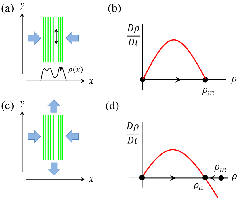
We next incorporate into the dynamics stretching in the $y$-direction, given by the rate $\gamma>0$, which is taken to be constant in position and time and independent of density. See Fig. 4c. This does not change Eq. (6), but modifies Eq. (8) to be

$$\frac{D}{Dt}\rho(x,t) =\frac{\partial}{\partial t}\rho+v\frac{\partial}{\partial x}\rho=\rho(\alpha-\gamma-\alpha\frac{\rho}{\rho_{m}})$$

$$=\alpha\rho\left(\frac{\rho_{a}-\rho}{\rho_{m}}\right),$$ (9)

where

$$\rho_{a}=\rho_{m}(\alpha-\gamma)/\alpha<\rho_{m}.$$ (10)

See Fig. 4d. With this modification, a parcel of material is driven toward the steady state density $\rho_{a}$ instead of $\rho_{m}$.

Note that the limit $\rho_{m}=\infty$, with $\alpha$ and $\gamma$ constant, removes the density dependence from Eqs. (6) and (9). Density then increases at the uniform rate of $\alpha-\gamma$ everywhere. This behavior is identical to the compression-stretching step for both the baker and Lozi maps, and it is well known that both of these maps have a fractal attractor, with a singular density distribution, but only when the system is contracting, i.e. $\alpha-\gamma>0$. This is not an accurate model for the microtubule-based system, which must be area-preserving on average. One could instead consider the incompressible limit of Eq. (9) by setting $\alpha=\gamma$. Though completely area-preserving dynamics will not produce fractal structure, it is possible to produce fractal structure if Step 1 is area preserving and it is combined with density fluctuations introduced in Step 3. (See Sect. III.3 below.) This special case is considered in Sect. V. Until then, we take $\rho_{m}$ to be finite.

Though area is not conserved locally in the microtubule system, we do require that area be conserved across the entirety of the material, as noted above. This means that the stretching rate must be balanced by the compression rate, i.e. $\gamma=-g(\bar{\rho}_{T})$, where $\bar{\rho}_{T}$ is the average density of the entire block of material. Since $\gamma$ is assumed constant in time, $\bar{\rho}_{T}$ must also be constant in time. Equation (9) then implies that

$$\bar{\rho}_{T}=\rho_{a}.$$ (11)

The “a” subscript stands for “average”.

By an appropriate choice of length and time scales, we can set $\alpha=\rho_{m}=1$ so that Eqs. (6) and (9) become

$$\frac{D}{Dt}\rho(x,t) =\frac{\partial}{\partial t}\rho+v\frac{\partial}{\partial x}\rho=\rho(r-\rho),$$ (12)

$$\frac{\partial v}{\partial x} =\rho-1,$$ (13)

where

$$r=\rho_{a}/\rho_{m}\leq 1$$ (14)

is dimensionless. Equation (11) for the density averaged over the entire material becomes

$$\bar{\rho}_{T}=r.$$ (15)

Note that there is no incompressible limit of Eqs. (12) and (13), since the rescaling assumes $\rho_{m}$ is finite.

III.2 Step 2: Folding dynamics

After the system has been compressed to one-half its original width, we introduce a fold. In the one-dimensional model, this means that the system returns to its original width $L_{0}$, with density

$$\rho(x,t)=\left\{\begin{array}[]{ll}\rho(x,t)&0<x<L_{0}/2,\\ \rho(L_{0}/2-x,t)&L_{0}/2<x<L_{0}.\end{array}\right.$$ (16)

An alternative perspective here is to extend $\rho(x,t)$ to an $x$-periodic function with wavelength $L_{0}$ that is also an even function in $x$. In this case, the function $\rho(x,t)$ will naturally evolve into the form of Eq. (16) once the original interval is compressed to half its length. Thus the fold step is naturally incorporated into the compression step.

To implement this step, we compute the time $T$ to compress the entire block of material from length $L_{0}$ to an arbitrary length $L$. First, assuming without loss of generality that the position of the left edge of the block is fixed at $x=0$, the velocity at the right edge $x=L$ is computed as

$$\frac{dL}{dt} =\int_{0}^{L}\frac{\partial v}{\partial x}dx=-\int_{0}^{L}(1-\rho)dx=-(1-r)L,$$ (17)

using Eqs. (13) and (15). Hence, the time to compress the block from $L_{0}$ to $L$ is

$$T=\frac{\log(L_{0}/L)}{1-r}=\frac{\log(2)}{1-r},$$ (18)

where in the final step we have set $L=L_{0}/2$.

III.3 Step 3: Imposing large-scale density variations

Immediately after the folding step we impose a multiplicate density variation $R(x)$ and normalize the density so that the average density remains $r$. Explicitly,

$$\rho(x)\mapsto\frac{R(x)\rho(x)}{\langle R(x)\rho(x)\rangle}r,$$ (19)

where the angled brackets denote the average over $x$. Consistent with the viewpoint that $\rho(x)$ is an even, $L_{0}$-periodic function, we similarly extend $R(x)$ to an even, $L_{0}$-periodic function.

III.4 Fractal generation

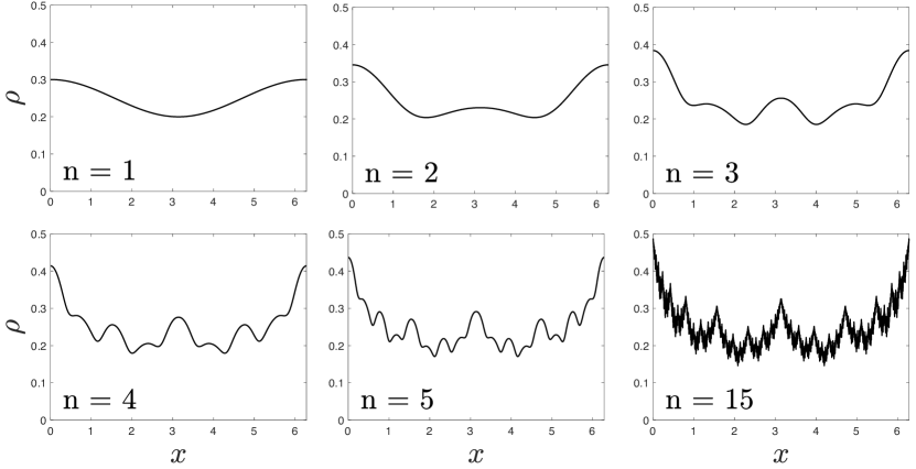
The sequence of compression by a factor of two, folding, and large-scale density variations generates a mapping $M$ of an original density $\rho_{0}(x)$ to a density $\rho(x)$; though the folding step can be ignored if $\rho(x)$ is even and $L_{0}$-periodic as discussed above. This mapping depends on the form $R(x)$ of the density variations imposed and the value of $r$ in the compression step. The mapping $M$ can then be repeatedly applied to the density. We numerically observe that it converges to a stationary fractal function, as seen in Fig. 5 for the density variation

$$R(x)=1+B\cos(x),$$ (20)

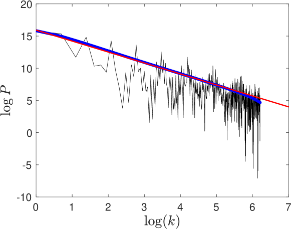
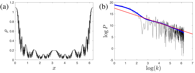
with $B=0.2$. Figure 6 shows the power spectrum (black) of the fractal image. The blue line is the power spectrum averaged over log(k), and the red line is a linear fit to this average. For comparison, Fig. 7 shows the stationary density distribution and power spectrum for larger amplitude density variations with $B=0.7$.

Figure 5: The density $\rho$ after each iterate $n$ of the map $M$ with $r=0.25$, $L_{0}=2\pi$, and density variation given by Eq. (20) with $B=0.2$. More and more fine-scale structure develops at each iterate. By $n=15$ the density has visually converged to an invariant state.

Figure 6: The power spectrum (black) of the final graph in Fig. 5 ($n=15$). The blue curve is the power spectrum smoothed according to Eq. (51). The smoothed spectrum is fit to a line (red) with slope -1.71.

IV Linear analysis of fractal generation

IV.1 Linearization of compression dynamics

The constant density

$$\rho_{0}(x,t)=r$$ (21)

and time-invariant velocity

$$v_{0}(x,t)=(r-1)x$$ (22)

are steady state solutions of Eqs. (12) and (13). Note that we have chosen a frame in which $v=0$ at the origin $x=0$. Expanding about this solution using

$$\rho =\rho_{0}+\epsilon g,$$ (23)

$$v =v_{0}+\epsilon f,$$ (24)

where $\langle g\rangle=0$, we find to first order in $\epsilon$

$$\frac{\partial}{\partial t}g =(1-r)x\frac{\partial}{\partial x}g-rg,$$ (25)

$$\frac{\partial f}{\partial x} =g.$$ (26)

Figure 7: a) The stationary density for the same parameters as Fig. 5, except $B=0.7$. b) The corresponding power spectrum. The fit slope $-1.60$ differs slightly from Fig. 6.

Note that the density perturbation $g$ decouples from $f$. Direct substitution shows that the solution to Eq. (25) for a given initial condition $g(x,0)$ has the form

$$g(x,t)=h(t)g(x/\ell(t),0),$$ (27)

where

$$\ell(t) =\exp((r-1)t),$$ (28)

$$h(t) =\exp(-rt).$$ (29)

This implies that the Fourier transform $\tilde{g}(k,t)$ evolves in time as

$$\tilde{g}(k,t)=h(t)\tilde{g}(k\ell(t),0).$$ (30)

Thus as time evolves, the graph of the power spectrum in log-log space shifts to larger wavenumbers and smaller amplitudes by translating along a line of slope $-2r/(r-1)$. After time $T$ given by Eq. (18), we find

$$\tilde{g}(k,T)=2^{-r/(1-r)}\tilde{g}(k/2,0).$$ (31)

This equation is valid when the Fourier transform is smooth, but must be treated carefully when the Fourier transform is singular, as when $\rho$ is $L_{0}$-periodic at $t=0$ and $t=T$. In this case $\tilde{g}(k,t)$ is zero except when $k=2\pi n/L_{0}$ for $n=0,1,2,3,...$, at which value it is a delta function whose amplitude we denote $\tilde{g}_{n}(t)$. These coefficients satisfy

$$\tilde{g}_{n}(T)=\left\{\begin{array}[]{ll}2^{-r/(1-r)}\tilde{g}_{n/2}(0),&n\text{ even}\\ 0,&n\text{ odd.}\end{array}\right.$$ (32)

Thus, the spacing between nonzero values of $\tilde{g}_{n}$ has increased by a factor of 2 over time $T$. Thus, when smoothed over $n$, as discussed in the Appendix, $|\tilde{g}_{n}|^{2}$ scales as

$$\langle|\tilde{g}_{n}(T)|^{2}\rangle \approx 0.5\times 2^{-2r/(1-r)}\langle|\tilde{g}_{\lfloor n/2\rfloor}(0)|^{2}\rangle$$

$$\approx 2^{-(1+r)/(1-r)}\langle|\tilde{g}_{\lfloor n/2\rfloor}(0)|^{2}\rangle,$$ (33)

where the angled brackets denote the average over $n$ and $\lfloor\quad\rfloor$ denotes the floor function. From this we see that the smoothed power spectrum $\langle|\tilde{g}_{n}(t)|^{2}\rangle$ slides down a line of slope $(1+r)/(1-r)$ in log-log space.

IV.2 Linearization of new density variations

We assume the density variations introduced by Eq. (19) scale as $\epsilon$, i.e.

$$R(x)=1+\epsilon p(x),$$ (34)

with $\langle p(x)\rangle=0$. Then, to first order in $\epsilon$ and using the expansion Eq. (23), Eq. (19) becomes

$$g(x)\mapsto g(x)+p(x),$$ (35)

which in terms of the Fourier coefficients, we write as

$$\tilde{g}_{n}\mapsto\tilde{g}_{n}+\tilde{p}_{n}.$$ (36)

IV.3 Linearized fractal generation

We denote by $A$ the linear operator that evolves $g(x,0)$ forward for time $T$ according to Eq. (27). Then the total linearized dynamics is

$$g\mapsto Ag+p.$$ (37)

Repeated application of this map, beginning with $g=0$ and using

$$p(x)=0.2\cos(x),$$ (38)

converges to the stationary function (blue) in Fig. 8, which is consistent with the nonlinear stationary density from Fig. 5 and reproduced in Fig. 8 (black). It is straightforward to see that

$$P=\sum_{m=0}^{\infty}A^{m}p,$$ (39)

is the unique invariant function of Eq. (37) and that any initial function will converge to it.

Figure 8: The invariant function (blue) obtained from repeated application of the linearized dynamics Eq. (37), with $r=0.25$ and $L_{0}=2\pi$. For comparison is the invariant function (black) obtained from the nonlinear dynamics and shown previously in Fig. 5.

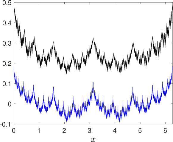
It was noted to us by S. Berman that when $p(x)$ is a cosine, as in Eq. (38), the invariant function $P(x)$ is the Weierstrass function, which was the first published example of a continuous function that is nowhere differentiable. Furthermore, fixed-point equations with the form of Eq. (37) were introduced by de Rham to characterize such singular functions. Such techniques have a history of applications to dynamical systems, e.g. Ref. Tasaki, Gilbert, and Dorfman, 1998.

In Fourier space, the linear operator $\tilde{A}$ that maps coefficients $\tilde{g}_{n}(0)$ forward to $\tilde{g}_{n}(T)$ is given by Eq. (32), and the invariant function is

$$\tilde{P}=\sum_{m=0}^{\infty}\tilde{A}^{m}\tilde{p},$$ (40)

with coefficients

$$\tilde{P}_{n}=\sum_{m=0}^{\infty}2^{-mr/(1-r)}\tilde{p}_{n/2^{m}},$$ (41)

where it is understood that $\tilde{p}_{n/2^{m}}=0$ if $n/2^{m}$ is not an integer.

Figure 9: The power spectrum (black) of the blue curve in Fig. 8. The blue curve above is the power spectrum smoothed according to Eq. (51). The smoothed spectrum is fit to a line (red) with slope -1.67.

Assuming that the density variation function $p(x)$ is analytic, its Fourier coefficients $\tilde{p}_{n}$ decay exponentially in $n$, meaning that the sum in Eq. (41) is dominated by the first nonzero term. This term will have an $m$ value satisfying $m\approx\log(n)/\log(2)$, and hence

$$\tilde{P}_{n}\propto n^{-r/(1-r)},$$ (42)

from which follows

$$|\tilde{P}_{n}|^{2}\propto n^{-2r/(1-r)},$$ (43)

and finally

$$\langle|\tilde{P}_{n}|^{2}\rangle\propto\frac{1}{n}n^{-2r/(1-r)}=n^{-(1+r)/(1-r)},$$ (44)

where the factor of $1/n$ that appears upon averaging is due to the diminishing density of nonzero coefficients, as discussed prior to Eq. (33). Thus in the linearized model, we find

$$\beta=\frac{1+r}{1-r}.$$ (45)

This is the same scaling that we previously identified for the temporal behavior in Eq. (33), highlighting the origin of this scaling in the compression dynamics.

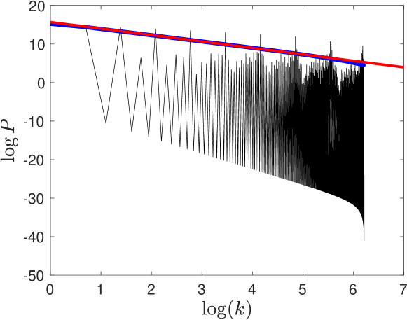
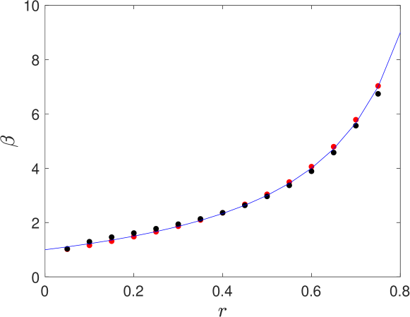
To check this formula numerically, we plot in Fig. 9 the power spectrum of the blue curve in Fig. 8, which has $r=0.25$. The linear fit yields a slope of $-1.67$, which agrees with the value $\beta=1.67$ obtained from Eq. (45). Figure 10 provides a more comprehensive comparison of the nonlinear analysis, the linear analysis, and Eq. (45). The black and red dots show $\beta$ versus $r$ for the nonlinear and linearized systems, respectively, using $R$ and $p$ given by Eqs. (20) (with $B=0.2$) and (38). The data are quite consistent with each other. The blue curve is the graph of Eq. (45), and it nicely tracks the red data points.

Figure 10: The variation of $\beta$ with $r$. The black dots are computed numerically from the nonlinear analysis with $B=0.2$. The red dots are computed numerically from the linear analysis. The blue curve is the graph of Eq. (45).

IV.4 The fluctuation injection scale

Figure 11: The (smoothed) power spectra of the linearized dynamics for three different sinusoidal forms for the injected density fluctuations. The black curve uses an injection wavelength equal to the full width of the material. The red and blue curves use wavelengths that are a factor of 10 and 100 smaller, respectively. The dashed vertical lines denote the scale of the injected density fluctuations. Note that the linear behavior only occurs when $k$ is greater than the injection value.

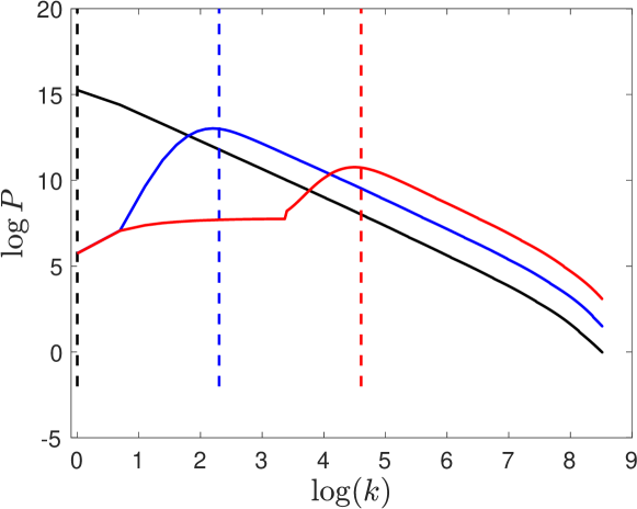
The value of $\beta$ does not depend on the details of the density fluctuations introduced by $p(x)$, except that its Fourier coefficients should fall off sufficiently rapidly. However, the $k^{-\beta}$ scaling only begins at length scales below the smallest length scale of $p(x)$. Figure 11 illustrates this by plotting the smoothed power spectrum for $p(x)$ with wavelengths equal to the width of the block of material divided by 1 [$p(x)=\cos(x)$, black], 10 [$p(x)=\cos(10x)$, blue], and 100 [$p(x)=\cos(100x)$, red]. These wavelengths are the scales at which density fluctuations are injected into the system. The $k$ value for each wavelength is denoted by the dashed vertical line of the corresponding color. The linear behavior only begins to the right of each line, i.e. at length scales smaller than the injection scale.

V The special case of incompressibility in Step 1

Returning to Eq. (9) and taking the limit $\rho_{m}=\infty$ and setting $\alpha=\gamma$, density is conserved in the Lagrangian frame,

$$\frac{D}{Dt}\rho(x,t)=0,$$ (46)

so that the material is incompressible, regardless of its density. Furthermore, Eq. (6) reduces to

$$\frac{\partial v}{\partial x}=-\alpha,$$ (47)

so that the system is uniformly compressed in the $x$ direction. Combining this with the density variations in Step 3, Eq. (19), we obtain a steady state fractal density. (We ignore subtle points about the convergence of this function, which is technically a distribution.) This dynamics is admittedly physically inconsistent, as we cannot imagine a situation in which density fluctuations could arrise via folding on the active scale (Step 3) without the material also being subject to compression or expansion in Step 1. Nevertheless, it is instructive to compute the resulting value of $\beta$, which is straightforward when linearizing the density fluctuations, i.e. using Eq. (34). Repeating the analysis in Sec. IV.3, one finds

$$\tilde{P}_{n}=\sum_{m=0}^{\infty}\tilde{p}_{n/2^{m}},$$ (48)

which simply reflects the fact that as a cosine density fluctuation is squeezed in $x$, its amplitude remains constant. This is the same result as Eq. (41) with $r=0$ and therefore gives the same power spectrum decay with $\beta=1$. Thus, even if one were to assume incompressibility in Step 1, the resulting value of $\beta$ disagrees with the experimental measurements in Fig. 3 (at least within the linearized analysis.)

VI Conclusions

By using a simple model of fractal generation, we have highlighted the necessity both of introducing density fluctuations on large scales and of a variable compressibility in the material. At least within the linearized analysis, the details of the density fluctuations are irrelevant to the value of $\beta$. The density fluctuations can take any functional form, so long as they have a minimum length scale. The $k^{-\beta}$ scaling then manifests at scales below this smallest length scale. In the case of the microtubule-based active nematic material, the injection scale of the density fluctuations is the active length scale of the system, i.e. the average defect spacing. Physically, the injected density variations are most naturally explained by the creation of defect pairs and the associated fracturing.

The $\beta$ parameter depends on the compressibility via $r$, and in the linearized analysis we derived an explicit relationship, Eq. (45). It is tempting to thus translate the experimentally measured values of $\beta$ (Fig. 3) into a material parameter $r$ via

$$r=\frac{\beta-1}{\beta+1},$$ (49)

yielding values of $r$ in the range $0.1$ – $0.3$. But what is the physical meaning of $r$? Within the context of the simple model, we can combine Eqs. (10) and (14), to rewrite $r$ as

$$r=1-\gamma/\alpha.$$ (50)

Recall $\gamma$ is the (uniform and constant) extension rate and $\alpha$ can be interpreted as the transverse compression rate in the low-density limit [Eq. (6)]. Whether this interpretation from the simple fractal model will hold for the actual laboratory system is not clear. This issue could be addressed via a realistic 2D hydrodynamic model with a density-dependent compressibility. Specifically, the dependence of $\beta$ on the material properties and system parameters would make an interesting and informative study.

Finally, it would be interesting to identify whether other physical systems exhibit a similar mechanism for fractal formation. Such systems would exhibit fractal structure not in the patterning of impurities mixed into the system, but in morphological properties such as density or surface texture. The classic example of chaos in a taffy puller comes to mind Thiffeault (2018), in which large-scale surface irregularities are introduced periodically by the folding of the taffy and then pushed down to smaller length scales by the stretching and compression dynamics.

DATA AVAILABILITY

The data that support the findings of this study are available from the corresponding author upon reasonable request.

Appendix A Spectral averaging

We smooth out local variations in a function $f(k)$ using a Gaussian function of width $\sigma$ in log space

$$\langle f\rangle(k)=\int_{0}^{\infty}f(k^{\prime})\frac{1}{N(k)}\exp\left[-\frac{1}{2\sigma^{2}}(\log k^{\prime}-\log k)^{2}\right]dk^{\prime},$$ (51)

with normalization

$$N(k) =\int_{0}^{\infty}\exp\left[-\frac{1}{2\sigma^{2}}(\log k^{\prime}-\log k)^{2}\right]dk^{\prime}$$

$$=\sqrt{2\pi}\sigma e^{\sigma^{2}/2}k.$$ (52)

Note that this smoothing preserves the $L^{1}$-norm, i.e. $\int_{0}^{\infty}|\langle f\rangle(k)|dk=\int_{0}^{\infty}|f(k)|dk$. Thus, spectral averaging of the power function preserves the total power. For all computations in this paper, we use $\sigma=0.4$.

References

- Marchetti et al. (2013) M. C. Marchetti, J. F. Joanny, S. Ramaswamy, T. B. Liverpool, J. Prost, M. Rao, and R. A. Simha, “Hydrodynamics of soft active matter,” Rev. Mod. Phys. 85, 1143–1189 (2013).
- Dell’Arciprete et al. (2018) D. Dell’Arciprete, M. L. Blow, A. T. Brown, F. D. C. Farrell, J. S. Lintuvuori, A. F. McVey, D. Marenduzzo, and W. C. K. Poon, “A growing bacterial colony in two dimensions as an active nematic,” Nature Communications 9, 4190 (2018).
- You et al. (2018) Z. You, D. J. G. Pearce, A. Sengupta, and L. Giomi, “Geometry and mechanics of microdomains in growing bacterial colonies,” Phys. Rev. X 8, 031065 (2018).
- Li et al. (2019) H. Li, X.-q. Shi, M. Huang, X. Chen, M. Xiao, C. Liu, H. Chaté, and H. P. Zhang, “Data-driven quantitative modeling of bacterial active nematics,” Proceedings of the National Academy of Sciences 116, 777–785 (2019), https://www.pnas.org/content/116/3/777.full.pdf .
- Saw et al. (2017) T. B. Saw, A. Doostmohammadi, V. Nier, L. Kocgozlu, S. Thampi, Y. Toyama, P. Marcq, C. T. Lim, J. M. Yeomans, and B. Ladoux, “Topological defects in epithelia govern cell death and extrusion,” Nature 544, 212 EP – (2017).
- Kawaguchi, Kageyama, and Sano (2017) K. Kawaguchi, R. Kageyama, and M. Sano, “Topological defects control collective dynamics in neural progenitor cell cultures,” Nature 545, 327 EP – (2017).
- Toner and Tu (1995) J. Toner and Y. Tu, “Long-range order in a two-dimensional dynamical model: How birds fly together,” Phys. Rev. Lett. 75, 4326–4329 (1995).
- Buhl et al. (2006) J. Buhl, D. J. T. Sumpter, I. D. Couzin, J. J. Hale, E. Despland, E. R. Miller, and S. J. Simpson, “From disorder to order in marching locusts,” Science 312, 1402–1406 (2006).
- Sanchez et al. (2012) T. Sanchez, D. T. N. Chen, S. J. DeCamp, M. Heymann, and Z. Dogic, “Spontaneous motion in hierarchically assembled active matter,” Nature 491, 431 EP – (2012).
- Ndlec et al. (1997) F. J. Ndlec, T. Surrey, A. C. Maggs, and S. Leibler, “Self-organization of microtubules and motors,” Nature 389, 305 EP – (1997).
- Henkin et al. (2014) G. Henkin, S. J. DeCamp, D. T. N. Chen, T. Sanchez, and Z. Dogic, “Tunable dynamics of microtubule-based active isotropic gels,” Philosophical Transactions of the Royal Society of London A: Mathematical, Physical and Engineering Sciences 372, 20140142 (2014).
- Giomi (2015) L. Giomi, “Geometry and topology of turbulence in active nematics,” Phys. Rev. X 5, 031003 (2015).
- DeCamp et al. (2015) S. J. DeCamp, G. S. Redner, A. Baskaran, M. F. Hagan, and Z. Dogic, “Orientational order of motile defects in active nematics,” Nature Materials 14, 1110 EP – (2015).
- Guillamat, Ignés-Mullol, and Sagués (2016) P. Guillamat, J. Ignés-Mullol, and F. Sagués, “Control of active liquid crystals with a magnetic field,” Proceedings of the National Academy of Sciences 113, 5498–5502 (2016), https://www.pnas.org/content/113/20/5498.full.pdf .
- Doostmohammadi et al. (2017) A. Doostmohammadi, T. N. Shendruk, K. Thijssen, and J. M. Yeomans, “Onset of meso-scale turbulence in active nematics,” Nature Communications 8, 15326 EP – (2017).
- Guillamat, Ignés-Mullol, and Sagués (2017) P. Guillamat, J. Ignés-Mullol, and F. Sagués, “Taming active turbulence with patterned soft interfaces,” Nature Communications 8, 564 (2017).
- Shendruk et al. (2017) T. N. Shendruk, A. Doostmohammadi, K. Thijssen, and J. M. Yeomans, “Dancing disclinations in confined active nematics,” Soft Matter 13, 3853–3862 (2017).
- Lemma et al. (2019) L. M. Lemma, S. J. DeCamp, Z. You, L. Giomi, and Z. Dogic, “Statistical properties of autonomous flows in 2d active nematics,” Soft Matter 15, 3264–3272 (2019).
- Tan et al. (2019) A. J. Tan, E. Roberts, S. A. Smith, U. A. Olvera, J. Arteaga, S. Fortini, K. A. Mitchell, and L. S. Hirst, “Topological chaos in active nematics,” Nature Physics 15 (2019), 10.1038/s41567-019-0600-y.
- Peitgen and Saupe (1988) H.-O. Peitgen and D. Saupe, eds., “The science of fractal images,” (Springer-Verlag, New York, 1988).
- Soille and Rivest (1996) P. Soille and J.-F. Rivest, “On the validity of fractal dimension measurements in image analysis,” Journal of Visual Communication and Image Representation 7, 217 – 229 (1996).
- Lopes and Betrouni (2009) R. Lopes and N. Betrouni, “Fractal and multifractal analysis: A review,” Medical Image Analysis 13, 634 – 649 (2009).
- Bies et al. (2016) A. J. Bies, C. R. Boydston, R. P. Taylor, and M. E. Sereno, “Relationship between fractal dimension and spectral scaling decay rate in computer-generated fractals,” Symmetry 8, 66 (2016).
- Nayak, Mishra, and Palai (2019) S. R. Nayak, J. Mishra, and G. Palai, “Analysing roughness of surface through fractal dimension: A review,” Image and Vision Computing 89, 21 – 34 (2019).
- Tel et al. (2005) T. Tel, A. de Moura, C. Grebogi, and G. Karolyi, “Chemical and biological activity in open flows: A dynamical system approach,” Phys. Rep. 413, 91–196 (2005).
- Aguirre, Viana, and Sanjuán (2009) J. Aguirre, R. L. Viana, and M. A. F. Sanjuán, “Fractal structures in nonlinear dynamics,” Rev. Mod. Phys. 81, 333–386 (2009).
- Lai and Tél (2010) Y.-C. Lai and T. Tél, Transient Chaos (Springer, New York, NY, 2010).
- Aref et al. (1989) H. Aref, S. Jones, S. Mofina, and I. Zawadzki, “Vortices, kinematics and chaos,” Physica D: Nonlinear Phenomena 37, 423–440 (1989).
- Muzzio et al. (1992) F. J. Muzzio, C. Meneveau, P. D. Swanson, and J. M. Ottino, “Scaling and multifractal properties of mixing in chaotic flows,” Physics of Fluids A: Fluid Dynamics 4, 1439–1456 (1992), https://doi.org/10.1063/1.858419 .
- Péntek et al. (1995) A. Péntek, Z. Toroczkai, T. Tél, C. Grebogi, and J. A. Yorke, “Fractal boundaries in open hydrodynamical flows: Signatures of chaotic saddles,” Phys. Rev. E 51, 4076–4088 (1995).
- Sandulescu et al. (2007) M. Sandulescu, C. López, E. Hernández-García, and U. Feudel, “Plankton blooms in vortices: the role of biological and hydrodynamic timescales,” Nonlinear Processes in Geophysics 14, 443–454 (2007).
- Truesdell et al. (2003) R. A. Truesdell, P. V. Vorobieff, L. A. Sklar, and A. A. Mammoli, “Mixing of a continuous flow of two fluids due to unsteady flow,” Phys. Rev. E 67, 066304 (2003).
- Phelan, Hughes, and Pathak (2008) F. R. Phelan, N. R. Hughes, and J. A. Pathak, “Chaotic mixing in microfluidic devices driven by oscillatory cross flow,” Physics of Fluids 20, 023101 (2008), https://doi.org/10.1063/1.2830550 .
- Alert, Joanny, and Casademunt (2020) R. Alert, J.-F. Joanny, and J. Casademunt, “Universal scaling of active nematic turbulence,” Nature Physics 16, 682–688 (2020).
- Hemingway et al. (2016) E. J. Hemingway, P. Mishra, M. C. Marchetti, and S. M. Fielding, “Correlation lengths in hydrodynamic models of active nematics,” Soft Matter 12, 7943–7952 (2016).
- Tasaki, Gilbert, and Dorfman (1998) S. Tasaki, T. Gilbert, and J. R. Dorfman, “An analytical construction of the srb measures for baker-type maps,” Chaos: An Interdisciplinary Journal of Nonlinear Science 8, 424–443 (1998), https://doi.org/10.1063/1.166324 .
- Thiffeault (2018) J.-L. Thiffeault, “The mathematics of taffy pullers,” The Mathematical Intelligencer 40, 26–35 (2018).