orvara: An Efficient Code to Fit Orbits using Radial Velocity, Absolute, and/or Relative Astrometry

Abstract

We present an open-source Python package, Orbits from Radial Velocity, Absolute, and/or Relative Astrometry (orvara), to fit Keplerian orbits to any combination of radial velocity, relative astrometry, and absolute astrometry data from the Hipparcos-Gaia Catalog of Accelerations. By combining these three data types, one can measure precise masses and sometimes orbital parameters even when the observations cover a small fraction of an orbit. orvara achieves its computational performance with an eccentric anomaly solver five to ten times faster than commonly used approaches, low-level memory management to avoid python overheads, and by analytically marginalizing out parallax, barycenter proper motion, and the instrument-specific radial velocity zero points. Through its integration with the Hipparcos and Gaia intermediate astrometry package htof, orvara can properly account for the epoch astrometry measurements of Hipparcos and the measurement times and scan angles of individual Gaia epochs. We configure orvara with modifiable .ini configuration files tailored to any specific stellar or planetary system. We demonstrate orvara with a case study application to a recently discovered white dwarf/main sequence (WD/MS) system, HD 159062. By adding absolute astrometry to literature RV and relative astrometry data, our comprehensive MCMC analysis improves the precision of HD 159062B’s mass by more than an order of magnitude to $0.6083^{+0.0083}_{-0.0073}\mbox{$M_{\sun}$}$. We also derive a low eccentricity and large semimajor axis, establishing HD 159062AB as a system that did not experience Roche lobe overflow.

1 Introduction

The history of orbit fitting extends back to ancient times, when it culminated in the Ptolemataic model of the Solar system. During the Age of Enlightenment astronomers fit the first Keplerian orbits to visual binary stars. More recently, masses derived from orbital fits, known as dynamical masses, anchor models of stellar evolution (Torres et al., 2010). Precise dynamical masses are used to infer the dynamical evolution of objects that reside off of the main sequence and rapidly evolve in the Hertzsprung-Russell diagram, such as young stars, brown dwarfs, giant planets and white dwarfs (Chabrier et al., 2000; Hillenbrand & White, 2004; Pala & Gänsicke, 2017).

Orbits have assumed a central role in exoplanet research, since exoplanets are often detected only through their effects on their host stars. For a planet detected by radial velocity monitoring, a Keplerian orbital fit may be the only observational result. Exoplanet demographics show that the mass distribution of companions has a gap between 10 $M_{\rm Jup}$ and 100 $M_{\rm Jup}$ (Zucker & Mazeh, 2001; Schlaufman, 2018), which suggests that exoplanets form very differently from low-mass stellar companions. Precise masses, along with luminosities and ages, provide a powerful way to test different planet formation mechanisms, substellar evolutionary models, and white dwarf cooling and atmospheric models (e.g. Benvenuto & Althaus, 1999; Martins & Palacios, 2017). Brown dwarfs and planets cool and fade with time: evolutionary models predict their luminosities as a function of age and mass (e.g. Burrows et al., 1997; Baraffe et al., 2003; Saumon & Marley, 2008). Systems with independent, dynamical masses provide the strongest tests and calibrations of these models (Crepp et al., 2016; Dupuy & Liu, 2017; Brandt et al., 2019; Maire et al., 2020).

For many years, orbital analyses focused on stars and used techniques appropriate for the computing power available. Some approaches used a grid search over a small number of parameters combined with linear least-squares fitting of the remaining parameters to map out $\chi^{2}$ surfaces (e.g., Hartkopf et al., 1989; Schaefer et al., 2006). Other common approaches used non-linear least-squares fitting to all parameters at once (e.g., Forveille et al., 1999; Gudehus, 2001) until Markov Chain Monte Carlo methods became more widespread (e.g., North et al., 2007; Ireland et al., 2008; Liu et al., 2008). In the meantime, orbital analysis has become central to the study of exoplanets, inspiring the development of many orbit-fitting tools over the last several years, including $\tt ExoFast$ (Eastman et al., 2013), $\tt PyAstrOFit$ (Wertz et al., 2016), BATMAN (Kreidberg, 2015), $\tt ExoSOFT$ (Mede & Brandt, 2017), $\tt RadVel$ (Fulton et al., 2018) and $\tt orbitize!$ (Blunt et al., 2020). In many cases, only one type of data (astrometry or radial velocity) is available to fit an orbit. Some of these tools, like BATMAN and RadVel, are designed with a particular data type in mind, while others including ExoSOFT and orbitize! are designed to deal with multiple data types. Multiple types of data can combine to offer much stronger constraints than any one type alone. Absolute astrometry from Hipparcos and Gaia is now capable of offering meaningful constraints (e.g., Pearce et al., 2020), especially when combined with relative astrometry and radial velocity measurements.

The Gaia spacecraft (Gaia Collaboration et al., 2016, 2018, 2020) has been surveying the nearby stellar or exoplanetary systems by taking photometric, spectroscopic and astrometric measurements across the sky with on-board instruments since 2014. The conceptually similar Hipparcos satellite (ESA, 1997; van Leeuwen, 2007) obtained astrometric measurements from 1989 to 1993. Hipparcos and Gaia measured the positions and motions of stars in an inertial reference frame called the International Celestial Reference System (ICRS) defined by distant quasars (Ma et al., 1998; Fey et al., 2015). The difference in their separate measurements of proper motions indicates acceleration in an inertial frame, which can be used to refine the orbital parameters of the accelerators. However, neither Hipparcos nor Gaia achieved a perfect realization of the ICRS, and both have low-level systematics and uncertainties that are sometimes underestimated. Brandt (2018) has cross-calibrated Hipparcos and Gaia DR2 to account for systematics as a function of position on the sky, putting them in the same reference frame. Brandt (2021) has performed a similar cross-calibration for Gaia EDR3.

Absolute astrometry can enable precise constraints on systems (Benedict et al., 2002, 2006) even when only a small fraction of the orbit is observed (Brandt et al., 2019). The combination of Gaia and Hipparcos proper motions provides a measurement of acceleration in the plane of the sky; a radial velocity trend adds a third dimension to the accelerations. Finally, direct imaging provides projected separations and position angles of the companions, allowing orbital constraints even without observing a substantial fraction of an orbit. Long-baseline precision RV surveys can identify stellar, substellar or planetary companions exhibiting accelerations, while a growing number of exoplanets are being discovered and characterized via high-contrast imaging (Marois et al., 2008; Lagrange et al., 2010; Rameau et al., 2013; Kuzuhara et al., 2013; Macintosh et al., 2015; Bowler, 2016).

Many authors have recently combined absolute astrometry with other data types to measure masses and orbits. These applications include radial velocity-detected exoplanets (Feng et al., 2019; Kervella et al., 2020; Damasso et al., 2020; Xuan & Wyatt, 2020; De Rosa et al., 2020), directly imaged planets and brown dwarfs (Calissendorff & Janson, 2018; Snellen & Brown, 2018; Dupuy et al., 2019; Brandt et al., 2019; Nielsen et al., 2020; Maire et al., 2020), and stars (Torres, 2019; Torres et al., 2019; Pearce et al., 2020). Our goal is to introduce a generalized, optimized, open source and flexible piece of software that can easily incorporate astrometric acceleration measurements.

In this paper, we present orvara, a Python Package designed for fast orbit-fitting and plotting of companions. We adopt a similar approach as Brandt et al. (2019) to jointly fit absolute astrometry, relative astrometry, and/or radial velocities of a given star and companion. Furthermore, we reduce the computational cost of our approach by introducing a more efficient eccentric anomaly solver, marginalizing out four or more nuisance parameters in the likelihood function, and using low-level memory management to avoid python overheads. orvara requires (and is distributed with) the Hipparcos-Gaia Catalog of Accelerations.

The paper is structured as follows. Section 2 reviews the basics of Keplerian orbits including equations that govern the measured positions and velocities as a function of time and corresponding orbital parameters. This is followed by a discussion of the implementation of these equations in orvara in Section 3. Section 4 describes the marginalized likelihood function over four or more parameters used in MCMC fitting. The computational performance of our implementation is examined in Section 5. The configuration and use of orvara, post-processing of the output, and plotting of a suite of eight plots relevant to astrometry and radial velocity are discussed in Section 6. We present a case study application of orvara to a recently discovered WD/MS system HD 159062 in Section 7 where new constraints on the companion mass and the eccentricity are presented. We conclude with our results and findings in Section 8.

2 Keplerian Orbits

A Keplerian orbit is a solution of the two-body problem for Newtonian gravity. It is fully described by six orbital elements plus the masses of the two components. We wish to use measured positions and velocities to derive posterior probability distributions on these eight parameters, marginalizing over several nuisance parameters (e.g., the position, parallax, and velocity of the system’s barycenter and astrophysical jitter in the measured radial velocities). In this section we briefly review the equations that give the measured positions and velocities as a function of time and the orbital parameters. We will describe our implementation of these equations and of the likelihood in subsequent sections.

In a Keplerian orbit, the mean anomaly $M$ varies linearly with time as

$$M=\frac{2\pi}{P}\left(t-t_{p}\right)$$ (1)

where $P$ is the system period and $t_{p}$ is the epoch of periastron passage. The position and velocity may be computed using the eccentric anomaly, which is given implicitly by

$$M=E-\varepsilon\sin E$$ (2)

where $\varepsilon$ is the eccentricity. The radial velocity RV is given through the true anomaly $\nu$ by

$$\nu =2\,{\rm atan2}\left[\sqrt{1+\varepsilon}\sin\frac{E}{2},\sqrt{1-\varepsilon}\cos\frac{E}{2}\right]$$ (3)

$${\rm RV} =k\left(\cos\left[\nu+\omega\right]+\varepsilon\cos\omega\right),$$ (4)

where $\omega$ is the argument of periastron, $k$ is the radial velocity amplitude, and ${\rm atan2}$ is the two-argument arctangent. We adopt a convention that the orbital parameters all refer to the companion(s). The orbital parameters for the primary are the same except that $\omega_{\rm pri}=\omega+\pi$.

The projected offset between the two bodies may be computed through the elliptical rectangular coordinates

$$X =\cos E-\varepsilon$$ (5)

$$Y =\left(\sin E\right)\sqrt{1-\varepsilon^{2}},$$ (6)

and the Thiele-Innes constants

$$A =\cos\Omega\cos\omega-\sin\Omega\sin\omega\cos i$$ (7)

$$B =\sin\Omega\cos\omega+\cos\Omega\sin\omega\cos i$$ (8)

$$F =-\cos\Omega\sin\omega-\sin\Omega\cos\omega\cos i$$ (9)

$$G =-\sin\Omega\sin\omega+\cos\Omega\cos\omega\cos i.$$ (10)

In Equations (7)–(10), $i$ is the inclination, and $\Omega$ is the longitude of the ascending node. The projected offsets of the secondary with respect to the primary star in declination $\Delta\delta$ and right ascension $\Delta\alpha*=\Delta(\alpha\cos\delta)$ are then given by

$$\Delta\delta =a(AX+FY)$$ (11)

$$\Delta\alpha* =a(BX+GY)$$ (12)

where $a$ is the semimajor axis in angular units.

Constraints on a system’s orbit may come from measurements of the primary star’s radial velocity over time, the projected angular offset of the two bodies, and/or the projected motion of either component relative to the system’s barycenter in an inertial reference frame. orvara is designed to account for all of these within the context of Gaussian uncertainties. While it is straightforward to apply Equations (4), (11), and (12) to compute predicted positions and velocities, implementing them as shown is typically inefficient and may require many trigonometric function calls per observational epoch. In the following sections we describe our computational implementation of the equations given in this section and our calculation of the likelihood.

3 Computational Implementation

3.1 The Eccentric Anomaly Solver

Equation (2) for the eccentric anomaly is known as Kepler’s Equation. Its importance, combined with its lack of an analytic solution, has inspired centuries worth of work on efficient computational approaches (e.g. Colwell, 1993, and references therein). A first-order Newton-Raphson approach requires an evaluation of sine and cosine at every iteration. Depending on the quality of the initial guess, this could result in anywhere from a few to $\approx$ten trigonometric evaluations per epoch. We have developed a more efficient approach for orvara: an eccentric anomaly solver based closely on that of Raposo-Pulido & Peláez (2017), hereafter RPP, with several modifications.

RPP’s basic approach is to obtain a very good initial guess for the eccentric anomaly through fitting formulae, followed by a single step of a modified Newton-Raphson method. We begin by reducing the range of the mean anomaly $M$ to $(-\pi,\pi]$; we further reduce the range to $[0,\pi]$ and save the sign of $M$ for later use. We then adopt the piecewise quintic fitting function for eccentric anomaly $E$ as a function of mean anomaly given in RPP, with the function values and the first two derivatives fixed where the eccentric anomaly is an integer multiple of $\pi/12$ (for twelve polynomials). Each polynomial $i$ is then defined over a range of mean anomalies $M_{i}$, $M_{i+1}$ given in Table 3 of RPP. To facilitate the calculation of the coefficients, we define the $i^{\rm th}$ quintic polynomial as

$$E\approx\sum_{k=0}^{5}a_{i,k}\left(M-M_{i}\right)^{k}$$ (13)

where $M_{i}$ is the minimum mean anomaly in the domain of the $i$-th quintic polynomial. With this definition,

$$a_{i,0} =E(M_{i}),$$ (14)

$$a_{i,1} =E^{\prime}(M_{i}),~{}~{}{\rm and}$$ (15)

$$a_{i,2} =\frac{1}{2}E^{\prime\prime}(M_{i}),$$ (16)

where the values and derivatives are tabulated in Table 3 of RPP. The other three coefficients may be derived by matching the values at $M_{i+1}$,

$$E(M_{i+1}) =\sum_{k=0}^{5}a_{i,k}\left(M_{i+1}-M_{i}\right)^{k},$$ (17)

$$E^{\prime}(M_{i+1}) =\sum_{k=1}^{5}a_{i,k}k\left(M_{i+1}-M_{i}\right)^{k-1},~{}~{}{\rm and}$$ (18)

$$E^{\prime\prime}(M_{i+1}) =\sum_{k=2}^{5}a_{i,k}k(k-1)\left(M_{i+1}-M_{i}\right)^{k-2}.$$ (19)

Since $a_{i,0}$, $a_{i,1}$, and $a_{i,2}$ are known from Equations (14)–(16), Equations (17)–(19) form a linear system of three equations for the three remaining coefficients. We solve this linear system by hand.

With a good initial guess for the eccentric anomaly $E$, we deviate very slightly from RPP and use Halley’s method to refine the solution for eccentricities $\varepsilon<0.78$. This requires the sine and cosine of the eccentric anomaly. We use a series expansion for one and a square root call for the other; these are significantly faster than trigonometric calls and remain within a factor of a few of double precision floating point accuracy. If $E<\pi/4$, we use the Taylor series for sine up to $15^{\rm th}$ order for a cost of seven additions and nine multiplications. We then compute $\cos E=\sqrt{1-\sin^{2}E}$, with no ambiguity in the sign given the range reduction. If $E>3\pi/4$, we use $\pi-E$ in the same Taylor expansion for sine. If $\pi/4<E<3\pi/4$, we use the identity $\cos E=\sin(\pi/2-E)$ and the Taylor expansion of sine to compute $\cos E$; we then use a square root call to evaluate $\sin E$.

For $\varepsilon<0.78$, a single iteration of Halley’s method brings the accuracy of our computed eccentric anomaly to nearly double precision. We then update $\sin E$ and $\cos E$, which we initially computed using series and square roots, with the summation trigonometric identities for $\sin(E+\delta E)$ and $\cos(E+\delta E)$. We evaluate $\sin\delta E$ and $\cos\delta E$ to second order in keeping with the second order accuracy of Halley’s method. Finally, we multiply $E$ and $\sin E$ by the sign of the mean anomaly. This brings $E$, $\sin E$, and $\cos E$ all close to double precision, with worst case errors below $10^{-15}$ for $\varepsilon<0.78$.

Figure 1: Left: residuals of the eccentric anomaly in radians, its sine and cosine, as a function of eccentricity for a uniform distribution of mean anomalies. The increasing errors in $E$ and $\sin E$ as $\varepsilon$ approaches unity are due to their mutual cancellation in Kepler’s equation: the residuals in $E-\varepsilon\sin E$ remain below $10^{-15}$. Right: time per epoch for the eccentric anomaly solvers in orvara, radvel (Fulton et al., 2018), the Nijenhuis (1991) solver of exoplanet (Foreman-Mackey et al., 2019), the goatherd/contour integral approach of Philcox et al. (2021), and batman (Kreidberg, 2015) using a single core of an Intel Xeon E5-2630, 2.2 GHz processor, and for 25, 100, or 500 epochs per eccentricity (dot-dashed, dashed, and solid lines, respectively). Our implementation of the Raposo-Pulido & Peláez (2017) algorithm includes the calculation of sine and cosine; we add a calculation of sine and cosine to the other methods. The dashed black curve shows the computational cost of a single call each to sine and cosine for each epoch. Our RPP implementation also has an additional overhead of $\sim$400 ns/orbit for the allocation and computation of the polynomials for the initial guess. This, combined with small Python overheads, accounts for the difference in cost between 25, 100, and 500 epochs.

At higher eccentricities, the initial polynomial guess behaves poorly when $M\ll 1$. If $2M+(1-\varepsilon)<0.2$, we adopt the second-order series expansion derived in RPP (their Equation (19)) for our starting point, and revert to the quintic polynomial fits otherwise. We find that at higher eccentricities and low mean anomalies, we sometimes require a third-order step to reach double precision accuracy in a single iteration. We therefore use Householder’s third-order method if both $\varepsilon>0.78$ and $M<0.4$, and Halley’s second-order method otherwise. As before, we refine $\sin E$ and $\cos E$ using the summation identities. Where $\varepsilon>0.78$ and $M<0.4$, we use series expansions up to third order to match the overall accuracy of Householder’s (third order) method. This approach is slightly slower than at lower eccentricities due to the higher-order variant of Newton’s method and to the need to occasionally use a series expansion for the initial guess. Up to eccentricities of 0.9999, however, the absolute errors in $E$ and $\sin E$ remain below $2\times 10^{-14}$ at all mean anomalies, and up to eccentricities of 0.99, they remain below $3\times 10^{-15}$ for all mean anomalies.

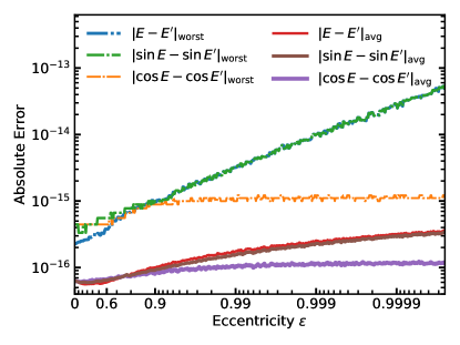
Figure 1 summarizes the performance of the eccentric anomaly solver. The left panel shows the overall accuracy, both the average and maximum errors as a function of eccentricity for a uniform distribution of eccentric anomalies. Even at an eccentricity of 0.9999 the algorithm is accurate to $2\times 10^{-14}$ in $E$ and $\sin E$, and to $10^{-15}$ in $\cos E$. The increasing error at high eccentricity is a result of a cancellation between $E$ and $\sin E$ in Kepler’s equation; it could be overcome by rewriting the equation in terms of $1-\varepsilon$ and expanding $\sin E$ as a series for small values of $E$. However, this would not solve the more fundamental problem that we can only compute the mean anomaly from the observation epoch with limited precision, and that $dE/dM$ can be large for $\varepsilon\approx 1$.

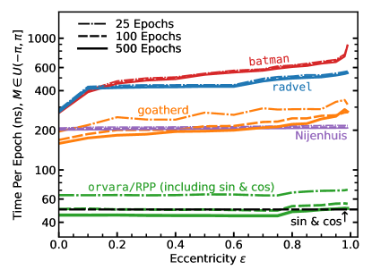
The right panel of Figure 1 shows the computational cost of our implementation of RPP compared to some other widely-used eccentric anomaly solvers, all evaluated on a single core of an Intel Xeon E5-2630, 2.2 GHz processor. Our implementation gives $\sin E$ and $\cos E$ as byproducts of the calculation. We add a call to sine and cosine when assessing other methods, as $\sin E$ and $\cos E$ are required to calculate radial velocities and/or positional offsets. There is an overhead of $\approx$170 ns associated with calculating the 72 polynomial coefficients at a given eccentricity, making the performance of our RPP implementation only slightly faster than other solvers for a single epoch. We have also implemented a version of this solver tailored to single epoch calculations. The single epoch version eliminates most of the overhead by constructing only one of the quintic polynomials (six coefficients). All methods shown in the right panel of Figure 1 also incur an overhead of a few hundred ns for the Cython function call. For 25 epochs at the same eccentricity, our implementation of RPP is around five times faster than these other approaches. With $\gtrsim$100 epochs at a given eccentricity, it can be faster than one call per epoch to both sine and cosine. Our implementation is $\sim$5–8 times faster than the SDG code (Raposo-Pulido & Peláez, 2017) because of its avoidance of explicit trigonometric calls and its approach to computing the polynomial coefficients.

3.2 Radial Velocities

Given the eccentric anomaly $E$, eccentricity $\varepsilon$, and radial velocity amplitude $k$, the radial velocity can be calculated by Equations (3) and (4). Written this way, the radial velocity evaluation requires five trigonometric calls (four if range reduction is used to enable the use of the single-argument arctangent). Only one of these, $\cos\omega$, can be computed once for all epochs in an orbit. However, Equations (3) and (4) are equivalent by trigonometric identities to

$$g =\left(\sqrt{\frac{1+\varepsilon}{1-\varepsilon}}\right)\left(\frac{1-\cos E}{\sin E}\right)$$ (20)

$${\rm RV} =k\left(\left(\frac{1-g^{2}}{1+g^{2}}+\varepsilon\right)\cos\omega-\left(\frac{2g}{1+g^{2}}\right)\sin\omega\right).$$ (21)

The quantities $\sin\omega$ and $\cos\omega$ appearing in Equation (21) only need to be computed once per orbit, not once per epoch. The quantities $\sin E$ and $\cos E$, needed for Equation (20), were already evaluated in the course of solving for the eccentric anomaly. Once $\sin\omega$ and $\cos\omega$ are computed for an orbit, computing the radial velocities using Equations (20) and (21) does not require a single trigonometric evaluation. In comparison tests, we found the use of Equations (20) and (21) to be $\sim$10–20 times faster than Equations (3) and (4).

Equation (20) can be problematic when $E\approx 0$. If $|E|<0.015$, we use the series expansion up to fifth order (there is no sixth order term); this gives a value of $g$ accurate to better than $10^{-15}$. If $E\approx\pm\pi$, Equation (21) presents no numerical problems unless $\sin E$ is precisely zero (in which case we simply set ${\rm RV}=k(\varepsilon-1)\cos\omega$).

3.3 Absolute and Relative Projected Positions

The relative offsets of the secondary from the primary star in right ascension $\alpha*$ and declination $\delta$ (where $\alpha*=\alpha\cos\delta$) are given by Equations (11) and (12). These equations present no computational difficulties. With $\sin E$ and $\cos E$ already computed from the eccentric anomaly solver, Equations (5)–(12) require five trigonometric evaluations plus one square root per orbit; zero per epoch.

We typically fit orbits using both absolute and relative astrometry. The displacement of the primary star from the system’s barycenter is related to the relative separations of Equations (11) and (12) by

$$\Delta\delta_{\star} =\left(\frac{-M_{\rm B}}{M_{\rm A}+M_{\rm B}}\right)\Delta\delta$$ (22)

$$\Delta\alpha*_{\star} =\left(\frac{-M_{\rm B}}{M_{\rm A}+M_{\rm B}}\right)\Delta\alpha*$$ (23)

where $M_{\rm A}$ is the mass of the primary star and $M_{\rm B}$ is the mass of its companion.

Astrometric missions like Hipparcos and Gaia measure the position of a star many times and fit an astrometric sky path. We use the Hundred Thousand Orbit Fitter (htof) (Brandt et al., 2021) to compute synthetic Hipparcos and Gaia catalog positions and proper motions from the offsets given in Equations (22) and (23). We then compare the htof synthetic catalog values to the cross-calibrated absolute astrometry of HGCA (Brandt, 2018). We refer the reader to the source code at https://github.com/gmbrandt/htof and the publication (when available) for further details.

3.4 Multiple Companions

Keplerian orbits only describe two-body systems. To fit more than one companion in orvara, we use a set of simplifying approximations that we describe here.

We approximate the star’s motion by a superposition of Keplerian orbits, one due to each companion. We use the orbital elements of each companion (shifting the argument of periastron by $\pi$ to give the stellar orbit), but we modify the total mass. For the mutual orbit between the star and a given companion indexed by $i$, we add the mass of all other companions that orbit closer to the star than companion $i$ itself. Effectively, we approximate the star and inner companions as a single body and solve for its motion about its barycenter due to the $i$-th companion. We then solve for the orbital motion within the inner system when we account for those companions. We add the contributions to the host star’s motion from all companions for both absolute astrometry and radial velocity.

We treat relative astrometry slightly differently. In this case, we ignore the influence of all companions orbiting beyond the companion of interest. We first compute the relative astrometry between this companion and the barycenter of the star and all inner companions. We then add the offset of the star relative to this barycenter due to the inner companions. This calculation is the same as the shift in absolute astrometry due to these inner companions.

These approximations do not fully capture interactions between companions. While incorrect in detail, our approach does capture some of the effects of a multi-body system. It can be used to fit extremely accurate relative astrometry (like that from GRAVITY, Gravity Collaboration et al. 2020), though not with the fidelity of a full (and expensive) suite of $N$-body simulations.

4 The Likelihood

We compute the likelihood ${\cal L}$ of an orbit as

$$-2\ln{\cal L}=\chi^{2}=\chi^{2}_{\rm RV}+\chi^{2}_{\rm rel\,ast}+\chi^{2}_{\rm abs\,ast}.$$ (24)

We treat $\chi^{2}_{\rm RV}$, the radial velocity component, first. We then take the latter two terms together as we marginalize out the barycenter’s proper motion and the system’s parallax.

4.1 Radial Velocity

For the radial velocity, we take

$$\chi^{2}_{\rm RV}=\sum_{j=1}^{N_{\rm inst}}\sum_{k=1}^{N_{\rm RV}}\bigg{(} \frac{\left({\rm RV}_{k}+{\rm ZP}_{j}-{\rm RV}\left[t_{k}\right]\right)^{2}}{\sigma^{2}[{\rm RV}_{k}]+\sigma^{2}_{\rm jit}}$$

$$\quad+\ln\left[\sigma^{2}[{\rm RV}_{k}]+\sigma^{2}_{\rm jit}\right]\bigg{)},$$ (25)

where ${\rm ZP}_{j}$ is the instrument-specific radial velocity zero point and $\sigma^{2}_{\rm jit}$ is a jitter term. We use ${\rm RV}_{k}$ to denote the measured RV at epoch $t_{k}$, ${\rm RV}[t_{k}]$ for the model-predicted RV and $\sigma^{2}[{\rm RV}_{k}]$ for its variance.

Our approach differs from Brandt et al. (2019) in that we adopt a single jitter for all instruments, attributing it to stellar activity. This has the disadvantage of assuming that instrumental uncertainties are properly estimated and that instruments sample similar regimes of stellar activity (the latter assumption could be problematic if combining visible and near-infrared data). However, it makes the fit robust to the inclusion of instruments with just a few data points, and it reduces the number of parameters to fit. orvara does include the option of fitting a different jitter to every RV instrument.

Equation (4.1) is the only place in the likelihood where the radial velocity zero point appears. We therefore marginalize it out, assuming a flat prior, by integrating

$${\cal L}\propto\int_{-\infty}^{\infty}d{\rm ZP}\exp\left[-\frac{\chi^{2}_{\rm RV}}{2}\right].$$ (26)

We perform the integral separately for each instrument. This requires only one pass through the radial velocity data set, and adds a negligible amount of computation. Performing the integral results in replacing $\chi^{2}_{\rm RV}$ with

$$\chi^{2}_{\rm RV}=\sum_{j=1}^{N_{\rm inst}} \left(-\frac{B_{j}^{2}}{4A_{j}}+C_{j}+\ln A_{j}\right)$$

$$+\sum_{j=1}^{N_{\rm inst}}\sum_{k=1}^{N_{\rm RV}}\ln\left[\sigma^{2}[{\rm RV}_{k}]+\sigma^{2}_{\rm jit}\right]$$ (27)

where

$$A_{j} =\sum_{k=1}^{N_{\rm RV}}\frac{1}{\sigma^{2}[{\rm RV}_{k}]+\sigma^{2}_{\rm jit}},$$ (28)

$$B_{j} =\sum_{k=1}^{N_{\rm RV}}\frac{2\left({\rm RV}_{k}-{\rm RV}\left[t_{k}\right]\right)}{\sigma^{2}[{\rm RV}_{k}]+\sigma^{2}_{\rm jit}},$$ (29)

$$C_{j} =\sum_{k=1}^{N_{\rm RV}}\frac{\left({\rm RV}_{k}-{\rm RV}\left[t_{k}\right]\right)^{2}}{\sigma^{2}[{\rm RV}_{k}]+\sigma^{2}_{\rm jit}},$$ (30)

and the sums over $k$ are restricted to radial velocity data points from instrument $j$. orvara uses Equations (27)–(30) as shown.

4.2 Astrometry

The $\chi^{2}$ for relative astrometry consists of two components: the relative separation $\rho$ and the position angle $\theta$ measured east of north. The model orbit’s relative separation is the product of the projected relative separation $\rho$ in AU and the system’s parallax $\varpi$. In general, the measurements of separation and position angle may be covariant: we take $c_{\rho\theta,k}\in(-1,1)$ to be the correlation coefficient between the two measurements at epoch $k$. The contribution to $\chi^{2}$ is then

$$\chi^{2}_{\rm rel\,ast} =\sum_{k=1}^{N_{\rm ast}}\frac{\lfloor\theta_{k}-\theta[t_{k}]\rfloor^{2}}{(1-c^{2}_{\rho\theta,k})\sigma^{2}[\theta_{k}]}+\sum_{k=1}^{N_{\rm ast}}\frac{\left(\rho_{k}-\varpi\rho\left[t_{k}\right]\right)^{2}}{(1-c^{2}_{\rho\theta,k})\sigma^{2}[\rho_{k}]}$$

$$\qquad-2\sum_{k=1}^{N_{\rm ast}}\frac{c_{\rho\theta,k}\lfloor\theta_{k}-\theta[t_{k}]\rfloor\left(\rho_{k}-\varpi\rho\left[t_{k}\right]\right)}{(1-c^{2}_{\rho\theta,k})\sigma[\theta_{k}]\sigma[\rho_{k}]}.$$ (31)

where $\rho_{k}$ and $\theta_{k}$ are the observed separation and position angle at time $t_{k}$, $\rho[t_{k}]$ and $\theta[t_{k}]$ are the model-predicted values, and $\lfloor\theta_{k}-\theta[t_{k}]\rfloor$ is the difference between the measured and the predicted position angles, reduced to the range $(-\pi,\pi]$.

The absolute astrometry in angular units is similarly proportional to parallax, and also has a velocity zero point. This is the proper motion of the system barycenter in the plane of the sky $\overline{\bm{\mu}}$, an almost perfect analog of the radial velocity zero point. This component of the likelihood then reads

$$\chi^{2}_{HG}= \left({\bm{\mu}_{H,\rm o}}-\overline{\bm{\mu}}-\varpi\bm{\mu}_{H}\right)^{T}{\bf C}_{H}^{-1}\left({\bm{\mu}_{H,\rm o}}-\overline{\bm{\mu}}-\varpi\bm{\mu}_{H}\right)$$

$$+\left({\bm{\mu}_{HG,\rm o}}-\overline{\bm{\mu}}-\varpi\bm{\mu}_{HG}\right)^{T}{\bf C}_{HG}^{-1}\left({\bm{\mu}_{HG,\rm o}}-\overline{\bm{\mu}}-\varpi\bm{\mu}_{HG}\right)$$

$$+\left({\bm{\mu}_{G,\rm o}}-\overline{\bm{\mu}}-\varpi\bm{\mu}_{G}\right)^{T}{\bf C}_{G}^{-1}\left({\bm{\mu}_{G,\rm o}}-\overline{\bm{\mu}}-\varpi\bm{\mu}_{G}\right)$$ (32)

where, e.g., $\bm{\mu}_{H,\rm o}$ is the observed Hipparcos proper motion and $\bm{\mu}_{H}$ is the model orbit’s predicted Hipparcos proper motion in AU yr^-1 (which must then be multiplied by the parallax to obtain a proper motion in angular units).

In some cases, Gaia obtains an astrometric solution for both stars in a binary. In this case, the observed epochs and scan angles will generally be the same for both stars, and the position and proper motion of the secondary may be easily computed from those of the primary. In the frame of the system barycenter (in which the orbit code operates), we have

$$\bm{\mu}_{\rm B}=-\bm{\mu}\left(\frac{M_{\rm A}}{M_{\rm B}}\right)$$ (33)

where $\bm{\mu}$ is the proper motion of the primary star and $\bm{\mu}_{\rm B}$ is the proper motion of its companion. Denoting the Gaia proper motion of the secondary by ${\bm{\mu}_{G,\rm o,B}}$, this measurement contributes an extra term to the astrometric $\chi^{2}$,

$$\Delta\chi^{2}_{HG}=\left({\bm{\mu}_{G,\rm o,B}}-\overline{\bm{\mu}}-\varpi\bm{\mu}_{G,\rm B}\right)^{T}{\bf C}_{G,\rm B}^{-1}\left({\bm{\mu}_{G,\rm o,B}}-\overline{\bm{\mu}}-\varpi\bm{\mu}_{G,\rm B}\right)$$ (34)

where ${\bf C}_{G,\rm B}^{-1}$ is the inverse of the Gaia covariance matrix for the secondary and $\overline{\bm{\mu}}$ remains the center-of-mass motion of the system’s barycenter. Including this additional term assumes that both stars have their proper motion in the same reference frame and have well-calibrated errors. Either assumption may break down in practice: Gaia DR2 has magnitude-dependent systematics in the reference frame of $\sim$0.2 mas yr^-1 (Figure 4 of Lindegren et al., 2018), while the HGCA required spatially variable error inflation by a typical factor $\sim$1.7 (Brandt, 2018). Gaia EDR3 retains magnitude-dependent systematics of up to $\approx$100 $\mu$as yr^-1 (Cantat-Gaudin & Brandt, 2021). We also neglect covariance between the secondary’s measured proper motion and the projected separation of the two bodies.

Equations (31) and (32) (with or without the additional term from Equation (34)) are quadratic equations in parallax and the two components of the proper motion of the system’s barycenter. We adopt a uniform prior on $\bm{\overline{\mu}}$, but use a Gaussian prior in parallax to incorporate the measured Gaia value. This is equivalent to adding one additional component to the log likelihood,

$$\chi^{2}_{\varpi}=\frac{\left(\varpi-\varpi_{\it Gaia}\right)^{2}}{\sigma_{\varpi,\it Gaia}^{2}}.$$ (35)

With the addition of Equation (35), we can write the design matrix of the system and solve for the maximum likelihood values of the parameters and their covariance matrix. Integrating the likelihood over parallax and barycentric proper motion is equivalent to substituting these maximum likelihood values into the expressions for $\chi^{2}$ and multiplying the likelihood by the square root of the determinant of the covariance matrix. This requires solving a $3\times 3$ linear system and computing the determinant of a $3\times 3$ matrix, neither of which incurs a significant computational cost. We write out this linear system in the Appendix. We solve the $3\times 3$ linear system using the singular value decomposition, but with a C routine to avoid the overheads associated with python function calls and memory management.

4.3 The Marginalized Likelihood

The integrations discussed in this section remove four parameters from the fit for a system when all radial velocities are from a single instrument, and more parameters otherwise. The computational cost of doing so is small relative to the cost of computing the orbit. The maximum posterior probability values of the parallax and barycenter proper motion may be of interest and are difficult to reconstruct from an output chain. We therefore save these quantities at each step for later use, along with the values for the Hipparcos, Hipparcos–Gaia, Gaia, relative separation, position angle components of $\chi^{2}$, and maximum likelihood radial velocity zero points of all instruments.

It is much more difficult to analytically integrate out other parameters. Wright & Howard (2009) show that the log likelihood can be linear in additional parameters if the parallax is accurately known. However, the priors on the combinations of parameters that enter the problem linearly can be complex even for simple choices of the underlying Keplerian parameters; the product of the likelihood and prior is difficult to integrate. Introducing relative astrometry (as we do for many of our targets) breaks the linearity entirely. If we consider parallax to be known, we may still integrate out the secondary mass if we adopt the total system mass as the other mass parameter in the problem, as long as we use a flat prior. Given these restrictions, we retain parallax as a linear parameter and do not analytically integrate out any others.

Our likelihood, after marginalizing four parameters, is a function of the six Keplerian orbital elements, the masses of the two components, and a radial velocity jitter, for a total of nine parameters. If there is more than one companion in the system, the likelihood becomes a function of two parameters (mass of the primary and radial velocity jitter) plus seven per companion (the six Keplerian orbital elements and the companion’s mass). We sample from this marginalized likelihood using the parallel-tempering MCMC sampler ptemcee (Vousden et al., 2016), a fork of emcee (Foreman-Mackey et al., 2013).

5 Performance

The computational cost of a single step includes contributions from the computation of the eccentric anomaly, the radial velocity and positional offsets, and the likelihood calculation. A typical data set consists of a few hundred measurements. Of these, $\sim$150–200 might be individual epochs from Hipparcos and Gaia. For a sample data set of Gl 758 (Brandt et al., 2019), there are 652 radial velocity measurements, 181 epochs for the absolute astrometry, and 4 epochs for relative astrometry. This data set requires 85 $\mu$s per iteration on a single core of a 2.2 GHz Intel Xeon E5-2630. Of this time, 44 $\mu$s is spent in the calculation of the eccentric anomalies, 5 $\mu$s on radial velocities, 2 $\mu$s on absolute astrometry for individual epochs, 9 $\mu$s on fitting the Hipparcos and Gaia models to the epoch astrometry, and 10 $\mu$s on the likelihood calculation. The remaining 15 $\mu$s are in overheads associated with emcee and the main python functions. For a sample data set of HD 4747, with 49 radial velocity measurements, 159 epochs for the absolute astrometry, and 8 epochs for relative astrometry, the total cost is $\sim$40 $\mu$s per iteration. Due to the smaller number of data points, the times spent calculating the eccentric anomaly, radial velocity, and likelihood fall to 11 $\mu$s, 1 $\mu$s, and 5 $\mu$s, respectively. The cost of fitting the Hipparcos and Gaia models to the epoch astrometry remains $\sim$9 $\mu$s. By comparison, a single-planet fit to 216 epochs of radial velocity data using radvel takes 1.0 ms per iteration with one core of the same CPU, or about 25 times slower than a fit to the same number of epochs (but with a diversity of data types) using orvara.

Overheads associated with allocating numpy arrays could take the majority of the computational time if we operated exclusively on arrays. We therefore explicitly handle memory allocation in Cython, and use C structures with pointers rather than numpy arrays. Replacing each pointer allocation with an ndarray and creating a memoryview would more than double the run time for HD 4747. For similar reasons, we use a C implementation of the singular value decomposition rather than a python call to the linear algebra routine in numpy. For a typical system with a few hundred observational epochs, the total computational cost to compute an orbit and evaluate its likelihood (marginalizing out parallax, radial velocity zero point, and barycenter proper motion) is equivalent to about three to seven trigonometric evaluations per epoch.

orvara uses the parallelization built into the packages emcee and ptemcee. The scaling under typical use is poor when using more than a handful of processors. Using five processors results in a speedup by just a factor of two on our machines, while adding further processors gives almost no additional speedup at all. Parallelization also works differently on different operating systems, and may not be supported on all machines. Regardless, multiple instances of the program may be run simultaneously for significantly better performance.

6 Configuration, Use and Plotting

orvara is an open-source Python package that performs parameter fits for multi-planetary or binary star systems using a combination of the Hipparcos-Gaia Catalog of Accelerations, literature radial velocities, and/or relative astrometry. orvara includes Python plotting routines to produce a comprehensive orbit-fitting and plotting package. It is available on GitHub. The detailed installation procedure of orvara and its updated documentation can be found in the $\tt README.rst$ file.

Most applications of orvara use radial velocity and/or relative astrometry data. Our example in Section 7 uses both. Each type of data is given in an input ASCII text file with fields separated by spaces or tabs; lines beginning with # are ignored. We provide examples in the repository and summarize their required structure in Table 1. The radial velocity file must include BJD, RV, and RV error (both in units of m/s) as its first three columns. An optional fourth column may include an integer $\geq$0 to distinguish instruments from one another; each instrument will have its own unique RV zero point. If the fourth column is not supplied orvara will assume that all radial velocities share the same zero point. The relative astrometry file must include date (either BJD or decimal year, with values $<$3000 interpreted as years), separation and its error (both in arcseconds), and position angle and its error (east of north, both in degrees) as its first five columns. An optional sixth column gives the correlation coefficient ($\in(-1,1)$) between separation and position angle. An optional seventh column gives the ID of the measured companion. The first companion is indexed as 0, the second as 1, etc. If the sixth and seventh columns are not supplied, orvara will use default values of 0 for each.

Table 1: Format of the input data files

Column Number	Description	Units	Required?	Default Value
Radial Velocity Data File
1	Observation epoch	BJD	yes	…
2	Radial velocity	m/s	yes	…
3	Radial velocity error	m/s	yes	…
4	RV instrument ID	…	no	0
Relative Astrometry Data File
1	Observation epoch	Decimal year or BJD	yes	…
2	Angular Separation	arcsec	yes	…
3	Separation error	arcsec	yes	…
4	Position angle (E of N)	degrees	yes	…
5	Position angle error	degrees	yes	…
6	Sep/PA correlation coefficient	…	no	0
7	Companion ID	…	no	0

Orbit fitting and plotting can be accessed with the $\tt fit\_orbit$ and $\tt plot\_orbit$ commands from the command line, respectively. The $\tt fit\_orbit$ output is a single Flexible Image Transport System (FITS) file (Wells et al., 1981) containing the MCMC chains and described in more detail below. The header of this FITS file includes the configuration parameters used to produce the chain. The $\tt plot\_orbit$ output is a suite of up to eight plots relevant to RV and relative astrometry and also discussed individually below. A star-specific .ini configuration file containing the appropriate file directories and settings serves as the input for both commands. This configuration file is comprised of four main sections denoted in square brackets: the data paths to all related file directories ($\tt[data\_paths]$), settings for MCMC fitting ($[\tt mcmc\_settings]$), settings for the primary mass prior and uncertainty ($\tt[priors\_settings]$), settings for plotting ($\tt[plotting]$), and for saving a table of results ($\tt save\_results$). A complete list of file directories and customizable input parameters including their descriptions and functionalities is provided in Table 2. Sample configuration files for Gl 758 and HD 4747, along with their sample data sets of radial velocity and relative astrometry, are included in the package. A user can omit data (for example, if there is no relative astrometry) by providing a blank or invalid file path. A user can also omit absolute astrometry by providing an invalid Hipparcos ID and supplying an explicit prior on the system parallax.

The first few lines in the .ini file specify the locations of data files and the Hipparcos ID of the primary star. The initial guesses for the nine MCMC parameters (plus seven for each companion beyond the first) may also be set in a file referenced in the .ini configuration file. orvara draws starting values for each walker from a normal or lognormal distribution with the means and variances specified. We assume log-flat priors for semimajor axis $a$, primary mass $\mathrm{M_{\rm pri}}$, companion mass $\mathrm{M_{\rm sec}}$, and radial velocity jitter $\mathrm{\sigma_{jit}}$; a prior of sini for inclination; and uniform priors for all other fitted parameters. Alternatively, the prior on the primary mass and its uncertainty can be set in $\tt[priors\_settings]$ to incorporate other knowledge of the star.

In addition to radial velocity fitting, we typically fit orbits using both absolute and relative astrometry (though only absolute astrometry is strictly required). Relative astrometry can be utilized by providing the data path to the relative astrometry file containing the astrometric epochs from different high-resolution imaging instruments. For epoch astrometry, the Hundred Thousand Orbit Fitter (htof Brandt et al., 2021) package mentioned in Section 3.3 is employed in orvara to provide parameter fits to the astrometric intermediate data from either Hipparcos data reduction or from Gaia. In order to use epoch astrometry, the file path to observational epochs and scan angles for Gaia, or to the intermediate data of Hipparcos (original or re-reduction) must be provided. The Gaia predicted scan epochs and angle can be queried using the Gaia Observation Forecast Tool, publicly available at $\mathrm{https://gaia.esac.esa.int/gost/index.jsp}$. htof parses the given intermediate data and extracts (inverse-)covariance matrices and epochs of observations to compute synthetic Hipparcos and Gaia catalog positions and proper motions described in Section 4.2.

The output of orvara is a single FITS file with the chain and other calculated parameters in a FITS table in header-data unit (HDU) 1. The header of the first extension (HDU 0) contains the configuration parameters read from the .ini file and used to construct the chain. The FITS table in HDU 1 contains columns with names, arrays, and units (where appropriate) for each fitted parameter, for the natural logarithm of the likelihood, and for other quantities computed at each step of the chain. Each array has dimensions ${\tt nwalkers}\times{\tt nstep//thin}$.

Table 2: Description of the configuration file contents.

Parameter Name	Data Type	Default	Description
[data_paths]
${\tt HipID}$	Integer	0	Hipparcos number. If valid, load HGCA absolute astrometry
${\tt HGCAFile}$	Data File	[required]	The Hipparcos-Gaia Catalog (either the DR2 or EDR3 edition)
${\tt RVFile}$	Data File	’’	File containing the radial velocity time series for the star
${\tt AstrometryFile}$	Data File	’’	File containing the relative astrometry for the companion(s)
${\tt GaiaDataDir}$	Directory	’’	Path to the Gaia scans as output by GOST in .csv format
${\tt Hip1DataDir}$	Directory	’’	Path to the Hipparcos (original reduction) intermediate data
${\tt Hip2DataDir}$	Directory	’’	Path to the Hipparcos (re-reduction) intermediate data
${\tt start\_file}$	Data File	’none’	File with the initial parameter guesses. If ’none’, use default guesses
[mcmc_settings]
${\tt ntemps}$	Integer	10	Number of temperatures to use in the parallel tempering chain
${\tt nwalkers}$	Integer	100	Number of walkers; each with ntemps number of chains
${\tt nplanets}$	Integer	[required]	Number of companions to fit
${\tt nstep}$	Integer	[required]	Number of steps contained in each chain
${\tt thin}$	Integer	50	Thinning of the chain (keep every ${\tt thin}$ step)
${\tt nthreads}$	Integer	1	Number of threads to use (the built-in parallelization is poor)
${\tt use\_epoch\_astrometry}$	Boolean	False	Use the epoch astrometry in GaiaDataDir, Hip1DataDir, etc.?
jit_per_inst	Boolean	False	Fit a separate RV jitter for each instrument?
[priors_settings]
${\tt mpri}$	Float	1	Mean of a Gaussian prior on primary mass (in $M_{\odot}$)
${\tt mpri\_sig}$	Float	inf	Uncertainty in the stellar priors. If inf, use the default $1/M$ prior
minjitter	Float	1e-5	Minimum allowable RV jitter (m/s). Should be $>0$
maxjitter	Float	1e3	Maximum allowable RV jitter (m/s). Must be $>{\tt minjitter}$
m_secondary0	Float	1	Mean (in $M_{\odot}$) of the (Gaussian) mass prior for companion 0
m_secondary0_sig	Float	1	Standard deviation of the (Gaussian) mass prior for companion 0
parallax	Float	None	Parallax prior: required if star is not in the HGCA, ignored otherwise
parallax_error	Float	None	Parallax prior if star is not in the HGCA
[secondary_gaia]			Gaia data of the secondary (set companion_ID = -1 if undetected)
companion_ID	Integer	-1	ID of the Gaia companion, should match entry in AstrometryFile
pmra	Float	0	Gaia proper motion (RA) of companion
pmdec	Float	0	Gaia proper motion (Dec) of companion
epmra	Float	1	Gaia proper motion uncertainty (RA) of companion
epmdec	Float	1	Gaia proper motion uncertainty (Dec) of companion
corr_pmra_pmdec	Float	0	Correlation ($\in(-1,1)$) between pmra and pmdec
[plotting]
${\tt McmcDataFile}$	Data File	[required]	Path to MCMC chain produced from the $\tt fit\_orbit$ command
${\tt burnin}$	Integer	0	Burnin length for thinned chains
${\tt check\_convergence}$	Boolean	False	Make diagnostic plots to help check for convergence?
iplanet	Integer	0	ID of the companion to plot ($0\leq{\tt iplanet}<{\tt nplanets}$)
${\tt target}$	String	’’	Name of the target, used for file naming
${\tt start\_epoch}$	Integer	1950	Customized range of dates (fractional years)
${\tt end\_epoch}$	Integer	2030	Customized range of dates (fractional years)
${\tt num\_orbits}$	Integer	50	Number of random orbits drawn from the posterior distribution
${\tt num\_steps}$	Integer	1000	Points per plotted orbit (aliasing can occur if num_steps is too small)
${\tt predicted\_years}$	Float(s)	2010,2020	Labeled year(s) on the best-fit orbit in the Astrometry plot
${\tt position\_predict}$	Float	2020	Epoch (fractional year) for the Astrometric_prediction_plot
${\tt Astrometry\_orbits\_plot}$	Boolean	True	Plot the astrometic orbits?
${\tt Astrometric\_prediction\_plot}$	Boolean	True	Plot the density plot for the predicted epoch?
${\tt RV\_orbits\_plot}$	Boolean	True	Plot the full RV orbits?
${\tt RV\_plot}$	Boolean	True	Plot RV orbits vs. epoch and O-C over the baseline of RV data?
${\tt RV\_Instrument}$	Integer/String	All	${\tt All}$ or Instrument number
${\tt Relative\_separation\_plot}$	Boolean	True	Plot relative separation vs. epoch and O-C?
${\tt Position\_angle\_plot}$	Boolean	True	Plot position angle vs. epoch and O-C?
${\tt Proper\_motion\_plot}$	Boolean	True	Plot the proper motions in RA and Dec and O-C?
${\tt Proper\_motion\_separate\_plots}$	Boolean	False	True if two separate plots for the proper motions are desired
${\tt Corner\_plot}$	Boolean	True	Plot a two dimensional corner plot from MCMC chain?
${\tt set\_limit}$	Boolean	False	Use user-specified axis limits?
${\tt xlim}$	Floats	None	If ${\tt set\_limit}$ is True, set x limits with two comma-separated values
${\tt ylim}$	Floats	None	If ${\tt set\_limit}$ is True, set y limits with two comma-separated values
${\tt marker\_color}$	String	blue	Matplotlib color of the marker for the observed data points
${\tt use\_colorbar}$	Boolean	True	Turn on/off colorbars.
${\tt colormap}$	String	viridis	Colormap name from the Matplotlib colormap library
${\tt reference}$	String	msec_jup	Colormap reference, ${\tt msec\_jup}$, ${\tt msec\_solar}$ or ${\tt ecc}$.
${\tt show\_title}$	Boolean	False	Turn on/off the title of the plot
${\tt add\_text}$	Boolean	False	True if adding text_name somewhere on the plot
${\tt text\_name}$	String	None	If ${\tt show\_title}$ is True, specify the text
${\tt x\_text}$	Float	None	If ${\tt add\_text}$ is True, enter the x coordinate of the text
${\tt y\_text}$	Float	None	If ${\tt add\_text}$ is True, enter the y coordinate of the text
[save_results]
${\tt save\_params}$	Boolean	True	Save the posterior parameters to a .txt file?
${\tt err\_margin}$	Float(s)	0.16,0.5,0.84	Quantiles for posterior parameters and uncertainties

We have implemented a plotting routine in Python to visualize the results obtained from the FITS file containing the MCMC chains produced by a joint orbit fit. In the $\tt[plotting]$ section of the .ini configuration file, the file path to the FITS file and a $\tt burnin$ length for the (thinned) MCMC chains must be specified. Also, users have the option to select which plots to generate using $\tt True$ and $\tt False$ values for the plot keywords. Here, we briefly describe the plots that orvara is currently configured to produce. Section 7 will provide an example fit and sample plots.

6.1 Astrometric orbits

The relative astrometric orbits for companions of stellar or planetary systems can be generated by setting $\tt Astrometry\_orbits\_plot$ to $\tt True$. Several features are worth mentioning in this plot. The thick black line indicates the highest likelihood orbits; thin lines are orbits randomly drawn from the posterior distributions and colored according to either the companion mass or eccentricity. This is the case for all the plots described below, except for the astrometric prediction plot which is a 2D contour. The black dashed line inside the most-likely orbit is the line of nodes joining the ascending node and the descending node of the most-likely orbit. This line of nodes indicates the position of the orbital plane of the system with respect to the sky plane. The unfilled circles plotted along the most-likely orbit are the predicted positions of the companion at specific user-defined epochs from $\tt predicted\_years$. If an astrometric file is provided from $\tt AstrometryFile$, the observations will be plotted as filled circles. If there is more than one companion included in the fit, the user may specify which one is plotted using the keyword iplanet (with $0\leq{\tt iplanet}<{\tt nplanets}$).

6.2 Astrometic prediction

orvara can predict the location of a companion relative to its host star at a specified epoch. The resulting density plot can be obtained by setting $\tt position\_predict$ to the desired epoch, and setting $\tt Astrometric\_prediction\_plot$ to $\tt True$. This contour plot shows the posterior probability density of the predicted positions of the companion in terms of relative offsets from the primary star in right ascension and declination, with the inner contour being the most likely position of the companion at that future epoch. The 1-$\sigma$, 2-$\sigma$, and 3-$\sigma$ contours enclose 68.3%, 95.4%, and 99.7% of the posterior probabilities for the future location.

6.3 Radial velocity orbits

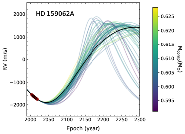
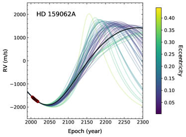
orvara can make two plots of the stellar radial velocity: one restricted to the observational time frame, and one spanning a longer, user-specified range of dates to show longer-term behavior. To make the latter plot the user may set $\tt RV\_orbits\_plot$ to $\tt True$. The former plot, restricted to the observational baseline, requires the user to give the path for $\tt RVFile$. The $\tt RVFile$ containing the observed radial velocity time series must have the format specified by Table 1. The filled circles on both plots represent RV data from all the radial velocity instruments. The observed RV data are shifted by an offset according to the maximum likelihood zero point for each RV instrument; the maximum likelihood offsets for each instrument are given by fields named, e.g., ‘RV_ZP_0_ML’ for instrument 0.

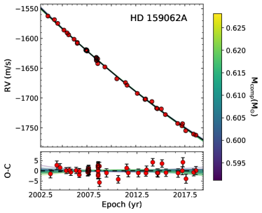
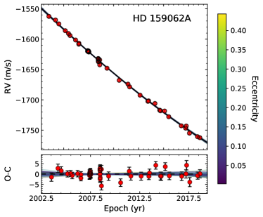
orvara can also make a plot of the RVs restricted to the time range sampled by the RV instruments; $\tt RV\_plot=True$ enables this plot. This is essentially a zoomed-in view of the part of the RV orbits plot described above. It contains RV data from single- or multi-instrument RV observations, plus a corresponding Observed$-$Calculated (hereafter O$-$C) residual shown underneath. To choose to plot the RVs from a specific or from all the RV instruments, users may set $\tt RV\_Instrument$ to the instrument number or to ‘All’. The observed data are represented by the solid circles with error bars. The O$-$C residual indicates both the deviation of the observed value from the most-likely orbit and the variation in RV across the orbits randomly drawn from the posterior. The error bars include the RV jitter of the best-fit orbit.

6.4 Relative separation and position angle

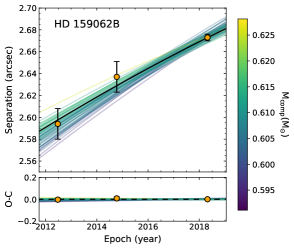
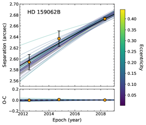
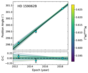
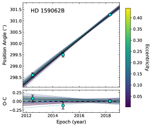
For relative astrometry, orvara offers two more plots in addition to the astrometric orbits plot: the relative separation (in arcseconds) and the position angle (in degrees) of the imaged companion relative to the primary star in a time range sampled by the relative astrometric instruments, and their corresponding O$-$C residuals. These two plots can be generated if the user sets $\tt Relative\_separation\_plot$ or $\tt Position\_angle\_plot$ to True. In each case, the path to $\tt AstrometryFile$ should be specified. The orbit’s relative separation in arcseconds is the product of the projected relative separation $\rho$ in AU and the parallax $\varpi$; we use the best-fit parallax for each set of orbital parameters. We refer the reader to Section 3.3 for a detailed description of the equations, and to the Appendix for the calculation of the best-fit parallax. The solid circles with error bars indicate the relative astrometric data from direct imaging instruments. Due to each instrument’s having different uncertainties, data reduction methods, and variations in the field rotation and plate scale, users may choose to adjust the imaging data in $\tt AstrometryFile$ to keep or discard a set of imaging data. Only one companion will be plotted. If there is more than one companion fit, the user may specify which one to plot using iplanet.

6.5 Proper motion

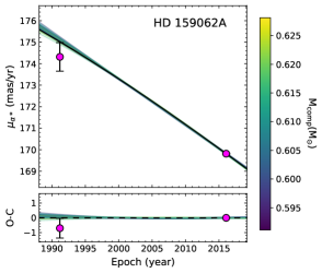
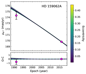
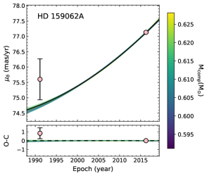
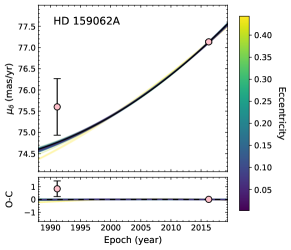
Variations in proper motion induced by the companion(s) on the primary star as measured from absolute astrometry from Hipparcos and Gaia can be plotted with $\tt Proper\_motion\_plot=True$. orvara computes these proper motions as instantaneous values using the time derivative of the eccentric anomaly. In contrast, both Hipparcos and Gaia fit sky paths to the star’s position as measured over several years. As a result, the observed data points and error bars do not correspond to the plotted lines in the same way that they do for, e.g., radial velocity. orvara does not plot the Hipparcos-Gaia mean proper motion, as this measurement does not represent an instantaneous proper motion at the mean epoch. It is, rather, a measurement of the integral of the proper motion. The O$-$C curves should be taken with caution. The actual $\chi^{2}$ values for each set of measurements (which are meaningful and also include measurement covariance) are available in the FITS file written by orvara.

To plot the two components of the proper motion as two separate, individual plots (one for right ascension and one for declination), users may set $\tt Proper\_motion\_separate\_plots$ to True. The data with error bars are from the cross-calibrated absolute astrometry of the HGCA. The HGCA provides three proper motions: one near 1991.25, another near 2015.5, and the positional difference between the Hipparcos re-reduction and the Gaia catalog (either the DR2 or EDR3 edition) scaled by the time between them. orvara plots data points for only the Hipparcos and Gaia proper motions. orvara adds the best-fit barycenter proper motion, calculated as described in the appendix, to each orbit.

6.6 Corner plot

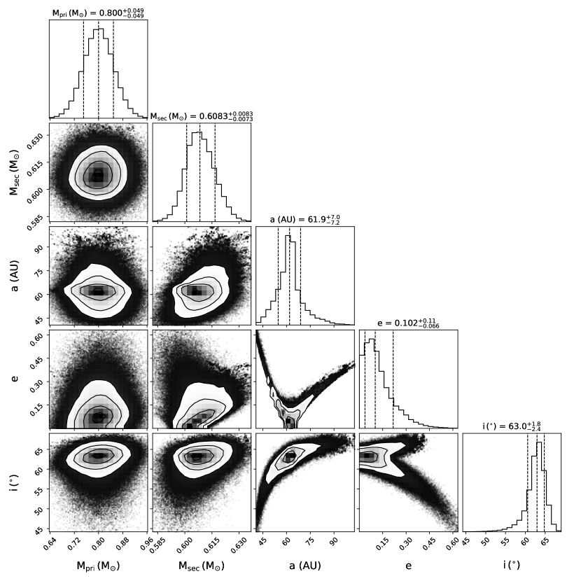
A two dimensional corner plot of the MCMC chain can be obtained by setting $\tt Corner\_plot$ to True. A $\tt burnin$ phase for the thinned MCMC chain can be specified for plotting. We have modified $\tt corner.py$ from Foreman-Mackey (2016) to format the titles displayed on top of the histograms in this plot. We chose to keep two significant figures in the uncertainties with a matching number of decimal places in the values.

The corner plot shows astrophysically meaningful Keplerian orbital elements including semi-major axis $a$, eccentricity $\varepsilon$, and inclination $i$, and the masses of the primary star in $M_{\sun}$ and its companion in $M_{\rm Jup}$ from the joint RV and astrometric MCMC analysis. If more than one companion is fit, the corner plot will use the parameters from the companion designated by iplanet.

7 Case study: application to HD 159062B

Table 3: HGCA proper motions

Source	$\mu_{\alpha*}$ (mas yr-1)	$\mu_{\delta}$ (mas yr-1)	corr	$t_{\alpha*}$	$t_{\delta}$	$\varpi$ (mas)	RV (km s-1)
Hipparcos	$174.316\pm 0.666$	$75.598\pm 0.612$	0.27	1991.20	1991.12
HG	$172.499\pm 0.019$	$75.776\pm 0.020$	0.11
Gaia EDR3	$169.814\pm 0.026$	$77.133\pm 0.029$	0.22	2016.07	2016.27	$46.118\pm 0.024$	$-84.11\pm 0.18$

In this section, we provide a case study application of orvara to a nearby white dwarf/main sequence (WD/MS) binary system, HD 159062. The white dwarf was discovered by Hirsch et al. (2019), hereafter H19, who fit for its orbit and mass. We first review the system, a widely-separated binary with a degenerate companion to a main sequence star, before summarizing the results of H19. We then discuss our own orbital fit and its implications for the binary system’s past evolution.

7.1 Background on HD 159062

Main sequence stars with masses $\lesssim$8 $M_{\sun}$ will evolve off the main sequence through the asymptotic giant branch (AGB) phase at the stellar evolutionary end-point and cool over billions of years until they eventually become dense white dwarfs (Dobbie et al., 2006). More than 97% of stars are expected to evolve into white dwarfs (Renedo et al., 2010). White dwarfs are used as powerful tools to trace the evolution of the Galaxy, and to provide constraints on global stellar populations. White dwarfs in binaries can also be potential progenitors of Type 1a supernovae (Hillebrandt & Niemeyer, 2000).

Spectroscopic and photometric surveys such as SDSS, Pan-STARRS and Gaia can reveal fundamental properties of white dwarfs including mass, cooling rate and age, and atmospheric and internal composition. The recent Gaia DR2 catalog has provided updated precise astrometric and photometric data that can be used to infer the local white dwarf population (Gentile Fusillo et al., 2019). Since most stars end their lives as WDs and most stars reside in binaries (Moe & Di Stefano, 2017), it is estimated that around one quarter of the more than two hundred known white dwarfs within 25 pc of the Sun reside in WD/MS or WD/WD binary systems (Holberg et al., 2016). Population synthesis modeling shows this number is reasonable but the observed rate of WD/MS binaries likely suffers from selection effects due to low detection sensitivity to faint white dwarfs near bright main sequence stars (Toonen, S. et al., 2017).

The host star of the system we study here, HD 159062A, is revealed spectroscopically as an old main sequence G-K dwarf star with low metallicity based on its $\log g$ and $T_{\rm eff}$ (H19). The observed Ca II HK emission $R^{{}^{\prime}}_{\rm HK}$ and rotation period led to an age diagnostic of $\sim$ 7 Gyr. Literature reports on HD 159062A’s age as derived from high-resolution spectroscopy range from approximately 5 Gyrs (e.g. Torres et al. (2019); Raghavan et al. (2012)) to 8 Gyrs (e.g. Pace (2013)) to 14 Gyrs (e.g. Luck (2017); Bai et al. (2018)).

Before the discovery of the white dwarf HD 159062B, Fuhrmann et al. (2017) predicted the existence of a degenerate companion around HD 159062A due to a barium overabundance of $[{\rm Ba/Fe}]=+0.4$ dex in HD 159062A. This is based on an empirical relation of the barium-to-iron enrichment as a function of age derived from an all-sky local population study of ancient Population II and intermediate-disk stars. Deviants from this Ba/Fe ratio versus age relation included five known stars with degenerate companions; HD 159062A was the most extreme outlier with an overabundance of barium. These five known systems almost certainly underwent mass transfer. Fuhrmann et al. (2017) characterize them as field blue stragglers due to high rotation, excessive chromospheric activity, lithium depletion, low orbital eccentricity and noticeable age discrepancies with activity-based age indicators (Fuhrmann & Bernkopf, 1999).

Solar-type Population II stars are old; they rotate at low rotational velocities and show low levels of chromospheric and coronal activity (Barnes, 2003; Mamajek & Hillenbrand, 2008). Additional observed chromospheric activity could be explained by mass and angular momentum transfer from binary companions. Many of the stars with degenerate companions studied by Fuhrmann et al. (2017) had slight barium depletions and $\lesssim$1000-day orbital periods, suggestive of mass transfer from first-ascent red giant progenitors. HD 159062, however, had an anomalously high Ba/Fe ratio unlikely to have arisen from a field anomaly at its formation epoch; it must have been instead due to the s-process nucleosynthesis product of a binary companion.

HD 159062’s overabundance of barium suggests wind accretion of s-process elements from a more distant AGB progenitor rather than Roche lobe overflow from first-ascent red giant progenitor (Boffin & Jorissen, 1988; Han et al., 1995; Jeffries & Stevens, 1996), so HD 159062B must have a longer period than $\sim$1000 days. Indeed, Fuhrmann et al. (2017) argue that barium enrichment via wind accretion only works for orbital periods from about 10 to 1000 years. This claim is backed up by an example of HD 114174, a cool white dwarf companion separated by $59.8\pm 0.4$AU from the G-type host star, whose orbital period is estimated to be between 154 and 881 years for eccentricities in the range 0$\leq$ e $\leq$ 0.5 (Matthews et al., 2014). A barium overabundance of $[{\rm Ba/Fe}]=+0.24$ dex is observed of the G star. The projected separation excludes the possibility of any substantial past mass exchange via Roche lobe overflow, however, Matthews et al. (2014) speculated that its orbit may have been pushed significantly outward during dynamical events such as the ejection of a third body.

The case of HD 114174 suggests a similar scenario for HD 159062, and the presence of a wide, white dwarf companion. HD 159062B could be located at a wider separation of tens of AUs away from HD 159062A whose observed barium overabundance can be explained by wind accretion of s-process materials from a former AGB primary that survived as a white dwarf companion, as well as any other dynamical events that may have widened its orbit. Apart from HD 114174 and HD 159062, Fuhrmann et al. (2017) also identified two systems, HR 3578 and 104 Tau, from their Ba/Fe ratio studies, both of which are without known companions but with slight barium anomalies. However, both stars’ lack of strong astrometric accelerations are not suggestive of any orbiting white dwarf companions at orbital periods of 10 - 1000 years. HR 3578 does show a $\sim$3$\sigma$ acceleration in declination in the HGCA. 104 Tau has been reported to be a visual binary (Eggen, 1956), but more recent interferometric non-detections (Raghavan et al., 2010), and stable radial velocities with a shallow trend (Butler et al., 2017) strongly suggest otherwise. HR 3578 and 104 Tau both represent good targets for follow-up imaging.

7.2 Data and Previous Fit

HD 159062B was discovered by H19 in 14 years of precise radial velocity (RV) data from the HIRES spectrograph on Keck (Vogt et al., 1994; Howard et al., 2010), and imaged using multi-epoch multi-band imaging observations from the ShaneAO system on the Lick Observatory 3-meter Shane telescope (Gavel et al., 2014; Srinath et al., 2014), the PHARO AO system on the Palomar Observatory 5-meter telescope (Hayward et al., 2001), and the NIRC2 AO system at the Keck II 10-meter telescope (Wizinowich et al., 2000). H19 performed a joint MCMC analysis using 45 radial velocities and three NIRC2 astrometric measurements to derive the best orbital parameters. They assumed Gaussian priors on the mass of the primary star, the difference between the pre-upgrade velocity zero point and the post-upgrade velocity zero point and parallax, and uniform priors on all other fitted parameters. H19 derived a new spectroscopic mass of $0.76\pm 0.03\mbox{$M_{\sun}$}$, but adopted a prior of $0.80\pm 0.05\mbox{$M_{\sun}$}$ based on literature values. H19 used 10 temperatures and 300 walkers in their MCMC in a total of $10^{5}$ steps. After the initial MCMC analysis, an additional prior on the white dwarf cooling age was added based on white dwarf cooling models and photometric constraints from ShaneAO, PHARO, and NIRC2s’ photometry measurements in $J$, $K_{s}$ and $L^{\prime}$. H19 concluded that the companion is an old $\mathrm{M_{B}=0.65^{+0.12}_{-0.04}\mbox{$M_{\sun}$}}$ with an orbital period of $P=250^{+130}_{-76}$ years, and a cooling age of $\mathrm{\tau=8.2^{+0.3}_{-0.5}}$ Gyr.

More recently, Bowler et al. (2021) performed an orbital fit using similar data and orvara with the DR2 version of the HGCA. Our results are similar to theirs, but are slightly more precise with the updated absolute astrometry from Gaia EDR3. We omit the additional RVs from Bowler et al. (2021) (which do not extend the observational baseline) and the additional relative astrometry. This enables a direct comparison of our results with those of H19 and shows the power of absolute astrometry to constrain the orbit of HD 159062AB.

7.3 A New Fit

We use orvara to perform a comprehensive joint MCMC analysis of HD 159062B using the same RV and imaging data as H19, but adding the cross-calibrated absolute astrometry of the HGCA. Table 3 summarizes the HGCA proper motions for HD 159062B, including the correlation coefficients between proper motions in right ascension and declination, and the central epoch for each measurement. The relative astrometry data are from three direct imaging instruments: ShaneAO, PHARO and NIRC2. Similarly to H19, we restrict our analysis to NIRC2 with its well-measured distortion correction and track record of precision astrometry (Service et al., 2016; Sakai et al., 2019).

Table 4: Basic Parameters and Default Priors

Parameter	Prior
RV Jitter $\sigma_{\rm jit}$	$1/\sigma$ (log-flat)
Primary Mass $M_{\rm pri}$	$1/M$ (log-flat)
Secondary Mass $M_{\rm sec}$	$1/M$ (log-flat)
Semimajor axis $a$	$1/a$ (log-flat)
$\sqrt{\varepsilon}\sin\omega$	uniform
$\sqrt{\varepsilon}\cos\omega$	uniform
Inclination $i$	$\sin(i)$, 0${}^{\circ}<i<180^{\circ}$
Mean longitude at 2010.0 $\lambda_{\rm ref}$	uniform
Ascending node $\Omega$	uniform
Parallax $\varpi$	$\exp[-\frac{1}{2}(\varpi-\varpi_{\it Gaia})^{2}/\sigma_{\varpi,\it Gaia}^{2}]$

Using orvara, we ran 10 temperatures and 100 walkers over $10^{5}$ steps to fit for nine parameters, keeping every 50^th step. Our results are based on the ‘coldest’ of 10 chains, with the ‘hottest’ chain being the chain that effectively samples all of the allowed parameter space. The total time taken using two cores was 2177 s $\sim$ 0.59 hr, and the mean acceptance fraction (cold chain) was 0.074. Table 4 provides a complete list of the parameters that we fit and the priors we used. We have marginalized out four parameters: the parallax $\varpi$, proper motion of the system barycenter, and RV offset as described in Section 4 and the Appendix.

Table 5: MCMC Results

Parameter	Median$\pm 1\sigma$	95.4% C.I.
Fitted parameters
RV Jitter $\sigma_{\rm jit}$ $({\rm m\,s}^{-1})$	${1.26}_{-0.30}^{+0.32}$	(0.65, 1.917)
Primary Mass $M_{\rm pri}$ $(M_{\odot})$	$0.80\pm 0.05$	(0.70, 0.90)
Secondary Mass $M_{\rm comp}$ $(M_{\odot})$	${0.608}_{-0.0073}^{+0.0083}$	(0.594, 0.625)
Semimajor axis $a$ (AU)	${61.9}_{-7.2}^{+7.0}$	(46.9, 83.3)
$\mathrm{\sqrt{e}\,sin\,\omega}$	${-0.17}_{-0.11}^{+0.15}$	($-$0.35, 0.13)
$\mathrm{\sqrt{e}\,cos\,\omega}$	${0.00\pm 0.32}$	($-$0.52, 0.55)
$\mathrm{Inclination}~{}i~{}(^{\circ})$	${63.0}_{-2.4}^{+1.8}$	(56.1, 66.6)
Mean longitude at $\mathrm{\lambda_{ref}~{}(^{\circ})}$	${151.5}_{-6.5}^{+8.0}$	(131.845, 167.314)
Ascending node $\mathrm{\Omega~{}(^{\circ})}$	${133.4}_{-1.3}^{+1.7}$	(130.97, 138.92)
Parallax $\varpi$ (mas)	$46.1856\pm 0.0042$	(46.177, 46.194)
Derived parameters
Period (years)	${411}_{-70}^{+71}$	(270, 641)
Argument of periastron $\omega\,(^{\circ})$	${260}_{-76}^{+70}$	(40, 348)
Eccentricity $\varepsilon$	${0.102}_{-0.066}^{+0.11}$	(0.006, 0.37)
Semimajor axis $a$ (mas)	${2862}_{-330}^{+320}$	(2170, 3850)
Time of periastron $T_{0}=\mathrm{t_{ref}}-P\frac{\lambda-\omega}{360^{\circ}}$ (JD)	${2506737}_{-31268}^{+16428}$	(2463393.772, 2583267.863)
Mass ratio	${0.761}_{-0.045}^{+0.050}$	(0.677, 0.866)

We examine the chains of each parameter to make sure that the burn-in phase was complete and all walkers had stabilized in the mean and standard deviation of the posterior.We discard the first 500 recorded steps (the first 25000 overall, as we save every 50^th) as the burn-in phase so that the chains are ready to be used for inference. The derived posterior probabilities from our joint orbit fit are given in Table 5. With this case study, we provide an example of the eight plots produced by orvara, described in Section 6. Two types of reference schemes are available for coloring the curves randomly drawn from the posterior distributions, either based on the mass of the secondary companion $M_{\rm sec}$ or eccentricity $\varepsilon$. We demonstrate both reference schemes for HD 159062B.

Figure 2: Relative astrometric orbits and predicted future position for HD 159062B. Left: relative astrometric orbits colored according to the secondary mass. Middle: relative astrometric orbits colored by eccentricity. Right: astrometric prediction of the location of HD 159062B in 2040. $\bf Left\,and\,Middle:$ the thick black lines indicate the highest likelihood orbit and the colorful thin lines from purple to yellow are 50 orbits drawn randomly from the posterior distributions colored according to the companion mass (left panel) or eccentricity (middle panel). The dotted lines connect the host star to the periastron passages. The black empty circles along the maximum likelihood deprojected orbit indicate epochs spaced by 10 years from 1990 to 2030. The dashed lines are the line of nodes. The filled orange circles are plotted along the maximum likelihood at the epochs corresponding to the relative astrometry used in our analysis. The arrows mark the direction of motion of the secondary companion. $\bf Right:$ The contour lines demonstrate the likelihood of the location of HD 159062B in 2040, ranging from light yellow (least likely) to red to black (most likely).

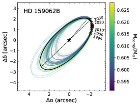
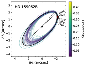
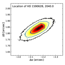
Figure 2 shows the astrometric orbit of HD 159062B. The RVs, both over a full orbit and restricted to the time frame of observations, are displayed in Figure 3. The relative separation and position angles of the companion HD 159062B with respect to the host star HD 159062A, and the absolute astrometry of the host star from HGCA are illustrated in Figure 4. Finally, to evaluate the full behavior of the joint posterior distributions, we show a corner plot of the derived parameters of HD 159062B in Figure 5.

Our joint orbit fit yields a companion mass of ${0.608}_{-0.0073}^{+0.0083}\mbox{$M_{\sun}$}$, an orbiting period of $P={411}_{-70}^{+71}$ years and an eccentricity of ${0.102}_{-0.066}^{+0.11}$ for the white dwarf HD 159062B. With our use of HGCA astrometry, we improve H19’s constraint on HD 159062B’s mass by an order of magnitude. Our tight constraints on the companion mass and eccentricity help to refine our picture of what the stellar system looks like. This can be used to infer the mass of the progenitor via the initial-final mass relation (Kalirai et al., 2008), which could serve as an input on the Barium enrichment of the primary star. We firmly place the system on the long period and low eccentricity tail of the distributions shown in Figure 6 of H19. This favors barium enrichment via wind accretion and rules out mass transfer by Roche lobe overflow. If the abundance measurement of $[{\rm Ba/Fe}]=0.4$ dex is accurate, HD 159062 would add to the few known cases of barium enrichment from wind accretion. This new information can be used to guide studies on the local stellar populations and Ba stars.

Figure 3: Top: RV orbits induced by the directly imaged companion over a significant fraction of its very long period, ranging from 1990 to 2280. Bottom: RVs and the observed-calculated residuals, restricted to the observational time frame. In all of the panels, the thick black line is the highest likelihood orbit and the colorful lines are 50 orbits randomly drawn from the posterior probability distribution for HD 159062B. They are colored according to secondary mass (left panels) or eccentricity (right panels). The red solid points with error bars are RV data from Keck/HIRES with the best-fit RV zero point added. Error bars are too small to be visible except for some points on the plot of residuals. An RV of zero represents the system’s barycentric velocity for the maximum likelihood orbit. The small bottom panel in each plot shows residuals after subtracting the RV orbit from the measurements. Due to the long orbital period of HD 159062B, more measurements are required to better constrain the orbital parameters. Moreover, we observe that with eccentricity as the reference coloring instead of the secondary mass, the RVs and residuals show more distinguishable structures. Lower eccentricity (more purple) orbits agree better with the highest likelihood orbit.

Figure 4: Observed and fitted relative and absolute astrometry for the HD 159062AB system. From top to bottom, the panels show the relative separation and position angle of HD 159062B, and the proper motion of HD 159062A in right ascension and declination. The thicker black lines represent the best-fit orbit in the MCMC chain while the other 50 lines represent random draws from the chain, color-coded by either companion mass (left panels) or eccentricity (right panels). The lower insets should the difference between observed and calculated astrometry. The mean proper motion is used to compute the MCMC chain, but is not shown in the proper motion plots. This constraint is an integral over the proper motion between the Hipparcos and Gaia epochs.

Figure 5: Corner plot of the derived parameters including mass of the primary star, mass of the secondary companion, semi-major axis, eccentricity, and inclination. The semimajor axis and eccentricity are highly covariant with one another and, to a lesser degree, with inclination.

8 Conclusions

In this paper, we have presented the orbit fitting package orvara, designed to fit one or more Keplerian orbits to any combination of radial velocity, relative astrometry, and absolute astrometry. orvara achieves high performance by using a combination of a fast eccentric anomaly solver (faster than a standalone call to sine and cosine for a large number of data points), analytic marginalization of parallax and barycenter proper motion, and low-level memory management. orvara is free and open-source. It depends on other free packages including emcee (Foreman-Mackey et al., 2013), ptemcee (Vousden et al., 2016), htof (Brandt et al., 2021), astropy (Astropy Collaboration et al., 2013; Price-Whelan et al., 2018), along with numpy (Oliphant, 2006; van der Walt et al., 2011) and scipy (Virtanen et al., 2020). orvara may be downloaded from github and installed by pip. We have tested its installation and operation on Windows, Mac and Linux machines.

We have demonstrated orvara on the system HD 159062, a white dwarf-main sequence binary discovered by Hirsch et al. (2019). Those authors found a white dwarf mass of $0.65_{-0.04}^{+0.12}~{}M_{\odot}$, and a semimajor axis and eccentricity that were compatible with a close pericenter passage. By combining absolute astrometry with the radial velocity and relative astrometry used by Hirsch et al. (2019), we improve the precision of the mass by an order of magnitude, to $0.617_{-0.012}^{+0.013}~{}M_{\odot}$. We exclude orbits with a close pericenter passage, establishing that the binary was a case of wind accretion system in its past.

orvara supports a variety of applications beyond what we have demonstrated here with HD 159062. It can account for multiple companions, it appropriately treats epoch astrometry from Hipparcos and/or Gaia, and it can account for a companion proper motion measured by Gaia. orvara is also designed to produce publication-ready plots. orvara may be configured with a single .ini file. We plan to keep orvara current, particularly when new Gaia data releases enable substantial improvements in astrometric precision.

$$\chi^{2}= \frac{\left(\varpi-\varpi_{\it Gaia}\right)^{2}}{\sigma^{2}_{\varpi,\it Gaia}}+\sum_{k=1}^{N_{\rm ast}}\frac{\left(\rho_{k}-\varpi\rho\left[t_{k}\right]\right)^{2}}{(1-c^{2}_{\rho\theta,k})\sigma^{2}[\rho_{k}]}-2\sum_{k=1}^{N_{\rm ast}}\frac{c_{\rho\theta,k}\lfloor\theta_{k}-\theta[t_{k}]\rfloor\left(\rho_{k}-\varpi\rho\left[t_{k}\right]\right)}{(1-c^{2}_{\rho\theta,k})\sigma[\rho_{k}]\sigma[\theta_{k}]}$$

$$+\left({\bm{\mu}_{H,\rm o,A}}-\overline{\bm{\mu}}-\varpi\bm{\mu}_{H}\right)^{T}{\bf C}_{H,\rm A}^{-1}\left({\bm{\mu}_{H,\rm o,A}}-\overline{\bm{\mu}}-\varpi\bm{\mu}_{H}\right)$$

$$+\left({\bm{\mu}_{HG,\rm o,A}}-\overline{\bm{\mu}}-\varpi\bm{\mu}_{HG}\right)^{T}{\bf C}_{HG,\rm A}^{-1}\left({\bm{\mu}_{HG,\rm o,A}}-\overline{\bm{\mu}}-\varpi\bm{\mu}_{HG}\right)$$

$$+\left({\bm{\mu}_{G,\rm o,A}}-\overline{\bm{\mu}}-\varpi\bm{\mu}_{G}\right)^{T}{\bf C}_{G,\rm A}^{-1}\left({\bm{\mu}_{G,\rm o,A}}-\overline{\bm{\mu}}-\varpi\bm{\mu}_{G}\right)$$

$$+\left({\bm{\mu}_{G,\rm o,B}}-\overline{\bm{\mu}}-\varpi\bm{\mu}_{G,\rm B}\right)^{T}{\bf C}_{G,\rm B}^{-1}\left({\bm{\mu}_{G,\rm o,B}}-\overline{\bm{\mu}}-\varpi\bm{\mu}_{G,\rm B}\right)$$ (1)

We can minimize $\chi^{2}$ with respect to parallax and proper motion of the barycenter by solving

$${\bf M}\begin{bmatrix}\varpi\\ \overline{\mu}_{\alpha*}\\ \overline{\mu}_{\delta}\end{bmatrix}={\bf b}$$ (2)

where $M$ is the symmetric matrix with elements

$$M_{\varpi\varpi} =\bm{\mu}_{H}^{T}{\bf C}_{H,\rm A}^{-1}\bm{\mu}_{H}+\bm{\mu}_{HG}^{T}{\bf C}_{HG,\rm A}^{-1}\bm{\mu}_{HG}+\bm{\mu}_{G}^{T}{\bf C}_{G,\rm A}^{-1}\bm{\mu}_{G}+\bm{\mu}_{G,\rm B}^{T}{\bf C}_{G,\rm B}^{-1}\bm{\mu}_{G,\rm B}+\frac{1}{\sigma^{2}_{\varpi,\it Gaia}}+\sum_{k=1}^{N_{\rm ast}}\frac{\rho^{2}\left[t_{k}\right]}{(1-c^{2}_{\rho\theta,k})\sigma^{2}[\rho_{k}]}$$ (3)

$$M_{\varpi\alpha} =\bm{\mu}_{H}\cdot\begin{bmatrix}C^{-1}_{H,{\rm A},\alpha\alpha}\\ C^{-1}_{H,{\rm A},\alpha\delta}\end{bmatrix}+\bm{\mu}_{HG}\cdot\begin{bmatrix}C^{-1}_{HG,{\rm A},\alpha\alpha}\\ C^{-1}_{HG,{\rm A},\alpha\delta}\end{bmatrix}+\bm{\mu}_{G}\cdot\begin{bmatrix}C^{-1}_{G,{\rm A},\alpha\alpha}\\ C^{-1}_{G,{\rm A},\alpha\delta}\end{bmatrix}+\bm{\mu}_{G,\rm B}\cdot\begin{bmatrix}C^{-1}_{G,{\rm B},\alpha\alpha}\\ C^{-1}_{G,{\rm B},\alpha\delta}\end{bmatrix}$$ (4)

$$M_{\varpi\delta} =\bm{\mu}_{H}\cdot\begin{bmatrix}C^{-1}_{H,{\rm A},\alpha\delta}\\ C^{-1}_{H,{\rm A},\delta\delta}\end{bmatrix}+\bm{\mu}_{HG}\cdot\begin{bmatrix}C^{-1}_{HG,{\rm A},\alpha\delta}\\ C^{-1}_{HG,{\rm A},\delta\delta}\end{bmatrix}+\bm{\mu}_{G}\cdot\begin{bmatrix}C^{-1}_{G,{\rm A},\alpha\delta}\\ C^{-1}_{G,{\rm A},\delta\delta}\end{bmatrix}+\bm{\mu}_{G,\rm B}\cdot\begin{bmatrix}C^{-1}_{G,{\rm B},\alpha\delta}\\ C^{-1}_{G,{\rm B},\delta\delta}\end{bmatrix}$$ (5)

$$M_{\alpha\alpha} =C^{-1}_{H,{\rm A},\alpha\alpha}+C^{-1}_{HG,{\rm A},\alpha\alpha}+C^{-1}_{G,{\rm A},\alpha\alpha}+C^{-1}_{G,{\rm B},\alpha\alpha}$$ (6)

$$M_{\delta\delta} =C^{-1}_{H,{\rm A},\delta\delta}+C^{-1}_{HG,{\rm A},\delta\delta}+C^{-1}_{G,{\rm A},\delta\delta}+C^{-1}_{G,{\rm B},\delta\delta}$$ (7)

$$M_{\alpha\delta} =C^{-1}_{H,{\rm A},\alpha\delta}+C^{-1}_{HG,{\rm A},\alpha\delta}+C^{-1}_{G,{\rm A},\alpha\delta}+C^{-1}_{G,{\rm B},\alpha\delta}$$ (8)

and ${\bf b}$ is given by

$$b_{\varpi} =\bm{\mu}_{H,\rm o}^{T}{\bf C}_{H,\rm A}^{-1}\bm{\mu}_{H}+\bm{\mu}_{HG,\rm o}^{T}{\bf C}_{HG,\rm A}^{-1}\bm{\mu}_{HG}+\bm{\mu}_{G,\rm o}^{T}{\bf C}_{G,\rm A}^{-1}\bm{\mu}_{G}+\bm{\mu}_{G,\rm o,B}^{T}{\bf C}_{G,\rm B}^{-1}\bm{\mu}_{G,\rm B}+\frac{\varpi_{\it Gaia}}{\sigma^{2}_{\varpi,\it Gaia}}$$

$$\qquad\qquad+\sum_{k=1}^{N_{\rm ast}}\frac{\rho_{k}\rho[t_{k}]}{(1-c^{2}_{\rho\theta,k})\sigma^{2}[\rho_{k}]}-\sum_{k=1}^{N_{\rm ast}}\frac{c_{\rho\theta,k}\rho[t_{k}]\lfloor\theta_{k}-\theta[t_{k}]\rfloor}{(1-c^{2}_{\rho\theta,k})\sigma[\rho_{k}]\sigma[\theta_{k}]}$$ (9)

$$b_{\alpha} =\bm{\mu}_{H,\rm o}\cdot\begin{bmatrix}C^{-1}_{H,{\rm A},\alpha\alpha}\\ C^{-1}_{H,{\rm A},\alpha\delta}\end{bmatrix}+\bm{\mu}_{HG,\rm o}\cdot\begin{bmatrix}C^{-1}_{HG,{\rm A},\alpha\alpha}\\ C^{-1}_{HG,{\rm A},\alpha\delta}\end{bmatrix}+\bm{\mu}_{G,\rm o}\cdot\begin{bmatrix}C^{-1}_{G,{\rm A},\alpha\alpha}\\ C^{-1}_{G,{\rm A},\alpha\delta}\end{bmatrix}+\bm{\mu}_{G,\rm o,B}\cdot\begin{bmatrix}C^{-1}_{G,{\rm B},\alpha\alpha}\\ C^{-1}_{G,{\rm B},\alpha\delta}\end{bmatrix}$$ (10)

$$b_{\delta} =\bm{\mu}_{H,\rm o}\cdot\begin{bmatrix}C^{-1}_{H,{\rm A},\alpha\delta}\\ C^{-1}_{H,{\rm A},\delta\delta}\end{bmatrix}+\bm{\mu}_{HG,\rm o}\cdot\begin{bmatrix}C^{-1}_{HG,{\rm A},\alpha\delta}\\ C^{-1}_{HG,{\rm A},\delta\delta}\end{bmatrix}+\bm{\mu}_{G,\rm o}\cdot\begin{bmatrix}C^{-1}_{G,{\rm A},\alpha\delta}\\ C^{-1}_{G,{\rm A},\delta\delta}\end{bmatrix}+\bm{\mu}_{G,\rm o,B}\cdot\begin{bmatrix}C^{-1}_{G,{\rm B},\alpha\delta}\\ C^{-1}_{G,{\rm B},\delta\delta}\end{bmatrix}.$$ (11)

The covariance matrix of $\varpi$ and the two components of $\overline{\bm{\mu}}$ is the inverse of ${\bf M}$. Integrating, or marginalizing, over $\overline{\bm{\mu}}$ and $\varpi$ is equivalent to replacing $\overline{\bm{\mu}}$ and $\varpi$ in Equation (1) with the solutions of Equation (2) and dividing by the square root of the determinant of ${\bf M}$ (multiplying by the square root of the determinant of the covariance matrix ${\bf M}^{-1}$).

References

- Astropy Collaboration et al. (2013) Astropy Collaboration, Robitaille, T. P., Tollerud, E. J., et al. 2013, A&A, 558, A33
- Bai et al. (2018) Bai, Y., Liu, J., Wicker, J., et al. 2018, ApJS, 235, 16
- Baraffe et al. (2003) Baraffe, I., Chabrier, G., Barman, T. S., Allard, F., & Hauschildt, P. H. 2003, A&A, 402, 701
- Barnes (2003) Barnes, S. A. 2003, ApJ, 586, 464
- Benedict et al. (2002) Benedict, G. F., McArthur, B. E., Forveille, T., et al. 2002, ApJ, 581, L115
- Benedict et al. (2006) Benedict, G. F., McArthur, B. E., Gatewood, G., et al. 2006, AJ, 132, 2206
- Benvenuto & Althaus (1999) Benvenuto, O. G., & Althaus, L. G. 1999, Monthly Notices of the Royal Astronomical Society, 303, 30
- Blunt et al. (2020) Blunt, S., Wang, J. J., Angelo, I., et al. 2020, The Astronomical Journal, 159, 89
- Boffin & Jorissen (1988) Boffin, H. M. J., & Jorissen, A. 1988, A&A, 205, 155
- Bowler (2016) Bowler, B. P. 2016, PASP, 128, 102001
- Bowler et al. (2021) Bowler, B. P., Cochran, W. D., Endl, M., et al. 2021, AJ, 161, 106
- Brandt et al. (2021) Brandt, G. M., Michalik, D., Brandt, T. D., et al. 2021, arXiv e-prints, arXiv:2109.06761
- Brandt (2018) Brandt, T. D. 2018, The Astrophysical Journal Supplement Series, 239, 31
- Brandt (2021) Brandt, T. D. 2021, ApJS, 254, 42
- Brandt et al. (2019) Brandt, T. D., Dupuy, T. J., & Bowler, B. P. 2019, AJ, 158, 140
- Burrows et al. (1997) Burrows, A., Marley, M., Hubbard, W. B., et al. 1997, ApJ, 491, 856
- Butler et al. (2017) Butler, R. P., Vogt, S. S., Laughlin, G., et al. 2017, AJ, 153, 208
- Calissendorff & Janson (2018) Calissendorff, P., & Janson, M. 2018, ArXiv e-prints, 1806.07899
- Cantat-Gaudin & Brandt (2021) Cantat-Gaudin, T., & Brandt, T. D. 2021, arXiv e-prints, arXiv:2103.07432
- Chabrier et al. (2000) Chabrier, G., Baraffe, I., Allard, F., & Hauschildt, P. 2000, The Astrophysical Journal, 542, 464
- Colwell (1993) Colwell, P. 1993, Solving Kepler’s equation over three centuries (Willman-Bell)
- Crepp et al. (2016) Crepp, J. R., Gonzales, E. J., Bechter, E. B., et al. 2016, ApJ, 831, 136
- Damasso et al. (2020) Damasso, M., Sozzetti, A., Lovis, C., et al. 2020, arXiv e-prints, arXiv:2007.06410
- De Rosa et al. (2020) De Rosa, R. J., Dawson, R., & Nielsen, E. L. 2020, A&A, 640, A73
- Dobbie et al. (2006) Dobbie, P. D., Napiwotzki, R., Burleigh, M. R., et al. 2006, Monthly Notices of the Royal Astronomical Society, 369, 383
- Dupuy et al. (2019) Dupuy, T. J., Brandt, T. D., Kratter, K. M., & Bowler, B. P. 2019, ApJ, 871, L4
- Dupuy & Liu (2017) Dupuy, T. J., & Liu, M. C. 2017, ApJS, 231, 15
- Eastman et al. (2013) Eastman, J., Gaudi, B. S., & Agol, E. 2013, PASP, 125, 83
- Eggen (1956) Eggen, O. J. 1956, AJ, 61, 405
- ESA (1997) ESA, ed. 1997, ESA Special Publication, Vol. 1200, The HIPPARCOS and TYCHO catalogues. Astrometric and photometric star catalogues derived from the ESA HIPPARCOS Space Astrometry Mission
- Feng et al. (2019) Feng, F., Anglada-Escudé, G., Tuomi, M., et al. 2019, MNRAS, 490, 5002
- Fey et al. (2015) Fey, A. L., Gordon, D., Jacobs, C. S., et al. 2015, The Astronomical Journal, 150, 58
- Foreman-Mackey (2016) Foreman-Mackey, D. 2016, The Journal of Open Source Software, 1, 24
- Foreman-Mackey et al. (2019) Foreman-Mackey, D., Czekala, I., Agol, E., Luger, R., & Barclay, T. 2019, dfm/exoplanet: exoplanet v0.2.4
- Foreman-Mackey et al. (2013) Foreman-Mackey, D., Hogg, D. W., Lang, D., & Goodman, J. 2013, PASP, 125, 306
- Forveille et al. (1999) Forveille, T., Beuzit, J.-L., Delfosse, X., et al. 1999, A&A, 351, 619
- Fuhrmann & Bernkopf (1999) Fuhrmann, K., & Bernkopf, J. 1999, A&A, 347, 897
- Fuhrmann et al. (2017) Fuhrmann, K., Chini, R., Kaderhandt, L., Chen, Z., & Lachaume, R. 2017, MNRAS, 471, 3768
- Fulton et al. (2018) Fulton, B. J., Petigura, E. A., Blunt, S., & Sinukoff, E. 2018, PASP, 130, 044504
- Gaia Collaboration et al. (2018) Gaia Collaboration, Brown, A. G. A., Vallenari, A., et al. 2018, A&A, 616, A1
- Gaia Collaboration et al. (2020) Gaia Collaboration, Brown, A. G. A., Vallenari, A., et al. 2020, arXiv e-prints, arXiv:2012.01533
- Gaia Collaboration et al. (2016) Gaia Collaboration, Prusti, T., de Bruijne, J. H. J., et al. 2016, A&A, 595, A1
- Gavel et al. (2014) Gavel, D., Kupke, R., Dillon, D., et al. 2014, in Society of Photo-Optical Instrumentation Engineers (SPIE) Conference Series, Vol. 9148, SPIE, 914805
- Gentile Fusillo et al. (2019) Gentile Fusillo, N. P., Tremblay, P. E., Gaensicke, B. T., et al. 2019, VizieR Online Data Catalog, J/MNRAS/482/4570
- Gravity Collaboration et al. (2020) Gravity Collaboration, Nowak, M., Lacour, S., et al. 2020, A&A, 633, A110
- Gudehus (2001) Gudehus, D. H. 2001, in American Astronomical Society Meeting Abstracts, Vol. 198, American Astronomical Society Meeting Abstracts #198, 47.09
- Han et al. (1995) Han, Z., Eggleton, P. P., Podsiadlowski, P., & Tout, C. A. 1995, Monthly Notices of the Royal Astronomical Society, 277, 1443
- Hartkopf et al. (1989) Hartkopf, W. I., McAlister, H. A., & Franz, O. G. 1989, AJ, 98, 1014
- Hayward et al. (2001) Hayward, T. L., Brandl, B., Pirger, B., et al. 2001, PASP, 113, 105
- Hillebrandt & Niemeyer (2000) Hillebrandt, W., & Niemeyer, J. C. 2000, ARA&A, 38, 191
- Hillenbrand & White (2004) Hillenbrand, L. A., & White, R. J. 2004, The Astrophysical Journal, 604, 741
- Hirsch et al. (2019) Hirsch, L. A., Ciardi, D. R., Howard, A. W., et al. 2019, ApJ, 878, 50
- Holberg et al. (2016) Holberg, J. B., Oswalt, T. D., Sion, E. M., & McCook, G. P. 2016, Monthly Notices of the Royal Astronomical Society, 462, 2295
- Howard et al. (2010) Howard, A. W., Johnson, J. A., Marcy, G. W., et al. 2010, ApJ, 721, 1467
- Ireland et al. (2008) Ireland, M. J., Kraus, A., Martinache, F., Lloyd, J. P., & Tuthill, P. G. 2008, ApJ, 678, 463
- Jeffries & Stevens (1996) Jeffries, R. D., & Stevens, I. R. 1996, MNRAS, 279, 180
- Kalirai et al. (2008) Kalirai, J. S., Hansen, B. M. S., Kelson, D. D., et al. 2008, ApJ, 676, 594
- Kervella et al. (2020) Kervella, P., Arenou, F., & Schneider, J. 2020, A&A, 635, L14
- Kreidberg (2015) Kreidberg, L. 2015, PASP, 127, 1161
- Kuzuhara et al. (2013) Kuzuhara, M., Tamura, M., Kudo, T., et al. 2013, ApJ, 774, 11
- Lagrange et al. (2010) Lagrange, A. M., Bonnefoy, M., Chauvin, G., et al. 2010, Science, 329, 57
- Lindegren et al. (2018) Lindegren, L., Hernandez, J., Bombrun, A., et al. 2018, arxiv, 1804.09366
- Liu et al. (2008) Liu, M. C., Dupuy, T. J., & Ireland, M. J. 2008, ApJ, 689, 436
- Luck (2017) Luck, R. E. 2017, AJ, 153
- Ma et al. (1998) Ma, C., Arias, E. F., Eubanks, T. M., et al. 1998, The Astronomical Journal, 116, 516
- Macintosh et al. (2015) Macintosh, B., Graham, J. R., Barman, T., et al. 2015, Science, 350, 64
- Maire et al. (2020) Maire, A. L., Baudino, J. L., Desidera, S., et al. 2020, A&A, 633, L2
- Mamajek & Hillenbrand (2008) Mamajek, E. E., & Hillenbrand, L. A. 2008, ApJ, 687, 1264
- Marois et al. (2008) Marois, C., Macintosh, B., Barman, T., et al. 2008, Science, 322, 1348
- Martins & Palacios (2017) Martins, F., & Palacios, A. 2017, A&A, 598, A56
- Matthews et al. (2014) Matthews, C. T., Crepp, J. R., Skemer, A., et al. 2014, The Astrophysical Journal, 783, L25
- Mede & Brandt (2017) Mede, K., & Brandt, T. D. 2017, AJ, 153, 135
- Moe & Di Stefano (2017) Moe, M., & Di Stefano, R. 2017, ApJS, 230, 15
- Nielsen et al. (2020) Nielsen, E. L., De Rosa, R. J., Wang, J. J., et al. 2020, AJ, 159, 71
- Nijenhuis (1991) Nijenhuis, A. 1991, Celestial Mechanics and Dynamical Astronomy, 51, 319
- North et al. (2007) North, J. R., Tuthill, P. G., Tango, W. J., & Davis, J. 2007, MNRAS, 377, 415
- Oliphant (2006) Oliphant, T. 2006, NumPy: A guide to NumPy, USA: Trelgol Publishing
- Pace (2013) Pace, G. 2013, A&A, 551, L8
- Pala & Gänsicke (2017) Pala, A. F., & Gänsicke, B. T. 2017, Astronomical Society of the Pacific Conference Series, Vol. 509, Dynamical Masses of Accreting White Dwarfs, ed. P. E. Tremblay, B. Gaensicke, & T. Marsh 91
- Pearce et al. (2020) Pearce, L. A., Kraus, A. L., Dupuy, T. J., et al. 2020, ApJ, 894, 115
- Philcox et al. (2021) Philcox, O. H. E., Goodman, J., & Slepian, Z. 2021, arXiv e-prints, arXiv:2103.15829
- Price-Whelan et al. (2018) Price-Whelan, A. M., Sipőcz, B. M., Günther, H. M., et al. 2018, AJ, 156, 123
- Raghavan et al. (2012) Raghavan, D., Farrington, C. D., ten Brummelaar, T. A., et al. 2012, ApJ, 745, 24
- Raghavan et al. (2010) Raghavan, D., McAlister, H. A., Henry, T. J., et al. 2010, ApJS, 190, 1
- Rameau et al. (2013) Rameau, J., Chauvin, G., Lagrange, A. M., et al. 2013, ApJ, 772, L15
- Raposo-Pulido & Peláez (2017) Raposo-Pulido, V., & Peláez, J. 2017, MNRAS, 467, 1702
- Renedo et al. (2010) Renedo, I., Althaus, L. G., Bertolami, M. M. M., et al. 2010, The Astrophysical Journal, 717, 183
- Sakai et al. (2019) Sakai, S., Lu, J. R., Ghez, A., et al. 2019, ApJ, 873, 65
- Saumon & Marley (2008) Saumon, D., & Marley, M. S. 2008, ApJ, 689, 1327
- Schaefer et al. (2006) Schaefer, G. H., Simon, M., Beck, T. L., Nelan, E., & Prato, L. 2006, AJ, 132, 2618
- Schlaufman (2018) Schlaufman, K. C. 2018, ApJ, 853, 37
- Service et al. (2016) Service, M., Lu, J. R., Campbell, R., et al. 2016, PASP, 128, 095004
- Snellen & Brown (2018) Snellen, I. A. G., & Brown, A. G. A. 2018, Nature Astronomy, 1808.06257
- Srinath et al. (2014) Srinath, S., McGurk, R., Rockosi, C., et al. 2014, in Society of Photo-Optical Instrumentation Engineers (SPIE) Conference Series, Vol. 9148, SPIE, 91482Z
- Toonen, S. et al. (2017) Toonen, S., Hollands, M., Gänsicke, B. T., & Boekholt, T. 2017, A&A, 602, A16
- Torres (2019) Torres, G. 2019, ApJ, 883, 105
- Torres et al. (2010) Torres, G., Andersen, J., & Giménez, A. 2010, A&A Rev., 18, 67
- Torres et al. (2019) Torres, G., Stefanik, R. P., & Latham, D. W. 2019, ApJ, 885, 9
- Torres et al. (2019) Torres, S., Cai, M. X., Brown, A. G. A., & Portegies Zwart, S. 2019, A&A, 629, A139
- van der Walt et al. (2011) van der Walt, S., Colbert, S. C., & Varoquaux, G. 2011, Computing in Science and Engineering, 13, 22
- van Leeuwen (2007) van Leeuwen, F. 2007, A&A, 474, 653
- Virtanen et al. (2020) Virtanen, P., Gommers, R., Oliphant, T. E., et al. 2020, Nature Methods, 17, 261
- Vogt et al. (1994) Vogt, S. S., Allen, S. L., Bigelow, B. C., et al. 1994, in SPIE, Vol. 2198, Instrumentation in Astronomy VIII, ed. D. L. Crawford & E. R. Craine, 362
- Vousden et al. (2016) Vousden, W. D., Farr, W. M., & Mandel, I. 2016, MNRAS, 455, 1919
- Wells et al. (1981) Wells, D. C., Greisen, E. W., & Harten, R. H. 1981, A&AS, 44, 363
- Wertz et al. (2016) Wertz, O., Absil, O., Gomez Gonzalez, C., et al. 2016, A&A, 598
- Wizinowich et al. (2000) Wizinowich, P., Acton, D. S., Shelton, C., et al. 2000, PASP, 112, 315
- Wright & Howard (2009) Wright, J. T., & Howard, A. W. 2009, ApJS, 182, 205
- Xuan & Wyatt (2020) Xuan, J. W., & Wyatt, M. C. 2020, arXiv e-prints, arXiv:2007.01871
- Zucker & Mazeh (2001) Zucker, S., & Mazeh, T. 2001, The Astrophysical Journal, 562, 1038