Unbiased Asymmetric Reinforcement Learning
under Partial Observability

Abstract.

In partially observable reinforcement learning, offline training gives access to latent information which is not available during online training and/or execution, such as the system state. Asymmetric actor-critic methods exploit such information by training a history-based policy via a state-based critic. However, many asymmetric methods lack theoretical foundation, and are only evaluated on limited domains. We examine the theory of asymmetric actor-critic methods which use state-based critics, and expose fundamental issues which undermine the validity of a common variant, and limit its ability to address partial observability. We propose an unbiased asymmetric actor-critic variant which is able to exploit state information while remaining theoretically sound, maintaining the validity of the policy gradient theorem, and introducing no bias and relatively low variance into the training process. An empirical evaluation performed on domains which exhibit significant partial observability confirms our analysis, demonstrating that unbiased asymmetric actor-critic converges to better policies and/or faster than symmetric and biased asymmetric baselines.

1. Introduction

(a) State.

(b) Observation.

Figure 1. Memory-Four-Rooms-9x9, a procedurally generated navigation task which requires information-gathering and memorization. The agent must avoid the bad exit and reach the good exit, which is identifiable by the color of the beacon.

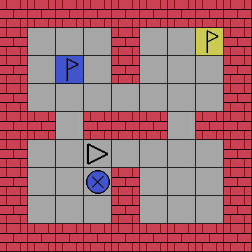
Partial observability is a key characteristic of many real-world reinforcement learning (RL) control problems where the agent lacks access to the system state, and is restricted to operate based on the observable past, a.k.a. the history. Such control problems are commonly encoded as partially observable Markov decision processes (POMDPs) Kaelbling et al. (1998), which are the focus of a significant amount of research effort. Offline learning/online execution is a common RL framework where an agent is trained in a simulated offline environment before operating online, which offers the possibility of using latent information not generally available in online learning, e.g., the simulated system state, or the state belief from the agent’s perspective Pinto et al. (2017); Karkus et al. (2018); Jonschkowski et al. (2018); Nguyen et al. (2020); Warrington et al. (2021); Chen et al. (2020).

Offline learning methods are in principle able to exploit this privileged information during training to achieve better online performance, so long as the resulting agent does not use the latent information during online execution. Specifically, actor-critic methods Sutton et al. (2000); Konda and Tsitsiklis (2000) are able to adopt this approach via critic asymmetry, where the policy and critic models receive different information Pinto et al. (2017); Foerster et al. (2018); Lowe et al. (2017); Li et al. (2019); Wang et al. (2020); Yang et al. (2018); Xiao et al. (2021), e.g., the history and latent state, respectively. This is possible because the critic is merely a training construct, and is not required or used by the agent to operate online. By the very nature of actor-critic methods, critic models which are unable or slow to learn accurate values act as a performance bottleneck on the policy. Consequently, critic asymmetry is a powerful tool which, if carried out with rigor, may provide significant benefits and bootstrap the agent’s learning performance.

Unfortunately, existing asymmetric methods use asymmetric information heuristically, and demonstrate their validity only via empirical experimentation on selected environments Pinto et al. (2017); Foerster et al. (2018); Lowe et al. (2017); Li et al. (2019); Wang et al. (2020); Yang et al. (2018); Rashid et al. (2018); Mahajan et al. (2019); Rashid et al. (2020); Nguyen et al. (2020); Xiao et al. (2021); the lack of a sound theoretical foundation leaves uncertainties on whether these methods are truly able to generalize to other environments, particularly those wich feature higher degrees of partial observability (see Figure 1). In this work, (a) we analyze a standard variant of asymmetric actor-critic and expose analytical issues associated with the use of a state critic, namely that the state value function is generally ill-defined and/or causes learning bias; (b) we prove an asymmetric policy gradient theorem for partially observable control, an extension of the policy gradient theorem which explicitly uses latent state information; (c) we propose a novel unbiased asymmetric actor-critic method, which lacks the analytical issues of its biased counterparts and is, to the best of our knowledge, the first of its kind to be theoretically sound; (d) we validate our theoretical findings through empirical evaluations on environments which feature significant amounts of partial observability, and demonstrate the advantages of our unbiased variant over the symmetric and biased asymmetric baselines.

This work sets the stage for other asymmetric critic-based policy gradient methods to exploit asymmetry in a principled manner, while learning under partial observability. Although we focus on advantage actor-critic (A2C), our method is easily extended to other critic-based learning methods such as off-policy actor-critic Degris et al. (2012); Wang et al. (2017), (deep) deterministic policy gradient Silver et al. (2014); Lillicrap et al. (2015), and asynchronous actor-critic Mnih et al. (2016). Offline training is also the dominant paradigm in multi-agent RL, where many asymmetric actor-critic methods could be similarly improved Foerster et al. (2018); Lowe et al. (2017); Li et al. (2019); Wang et al. (2020); Yang et al. (2018); Rashid et al. (2018); Mahajan et al. (2019); Rashid et al. (2020); Xiao et al. (2021).

2. Related Work

The use of latent information during offline training has been successfully adopted in a variety of policy-based methods Pinto et al. (2017); Foerster et al. (2018); Lowe et al. (2017); Yang et al. (2018); Li et al. (2019); Wang et al. (2020); de Witt et al. (2021); Warrington et al. (2021); Xiao et al. (2021) and value-based methods Rashid et al. (2018); Mahajan et al. (2019); Rashid et al. (2020); de Witt et al. (2021). Among the single-agent methods, asymmetric actor-critic for robot learning Pinto et al. (2017) uses a reactive variant of DDPG with a state-based critic to help address partial observability; belief-grounded networks Nguyen et al. (2020) use a belief-reconstruction auxiliary task to train history representations; and Warrington et al. Warrington et al. (2021) and Chen et al. Chen et al. (2020) use a fully observable agent trained offline on latent state information to train a partially observable agent via imitation.

Asymmetric learning has also become popular in the multi-agent setting: COMA Foerster et al. (2018) uses reactive control and a shared asymmetric critic which can receive either the joint observations of all agents or the system state to solve cooperative tasks; MADDPG Lowe et al. (2017) and M3DDPG Li et al. (2019) use the same form of asymmetry with individual asymmetric critics to solve cooperative-competitive tasks; R-MADDPG Wang et al. (2020) uses recurrent models to represent non-reactive control, and the centralized critic uses the entire histories of all agents; CM3 Yang et al. (2018) uses a state critic for reactive control; while ROLA Xiao et al. (2021) trains centralized and local history/state critics to estimate individual advantage values. Asymmetry is also used in multi-agent value-based methods: QMIX Rashid et al. (2018), MAVEN Mahajan et al. (2019), and WQMIX Rashid et al. (2020) all train individual Q-models using a centralized but factored Q-model, itself trained using state, joint histories, and joint actions.

3. Background

In this section, we review background topics relevant to understand our work, i.e., POMDPs, the RL graphical model, standard (symmetric) actor-critic, and asymmetric actor-critic.

Notation

We denote sets with calligraphy $\mathcal{X}$, set elements with lowercase $x\in\mathcal{X}$, random variables (RVs) with uppercase $X$, and the set of distributions over set $\mathcal{X}$ as $\Delta\mathcal{X}$. Occasionally, we will need absolute and/or relative time indices; We use subscript $x_{t}$ to indicate absolute time, and superscript $x^{(k)}$ to indicate the relative time of variables, e.g., $x^{(0)}$ marks the beginning of a sequence happening at an undetermined absolute time, and $x^{(k)}$ is the variable $k$ steps later. We also use the bar notation to represent a sequence of superscripted variables $\bar{x}=(x^{(0)},x^{(1)},x^{(2)},\ldots)$.

3.1. POMDPs

A POMDP Kaelbling et al. (1998) is a discrete-time partially observable control problem determined by a tuple $\langle\mathcal{S},\mathcal{A},\mathcal{O},T,O,R,\gamma\rangle$ consisting of: state, action and observation spaces $\mathcal{S}$, $\mathcal{A}$, and $\mathcal{O}$; transition function $T\colon\mathcal{S}\times\mathcal{A}\to\Delta\mathcal{S}$; observation function $O\colon\mathcal{S}\times\mathcal{A}\times\mathcal{S}\to\Delta\mathcal{O}$; reward function $R\colon\mathcal{S}\times\mathcal{A}\to\mathbb{R}$; and discount factor $\gamma\in\left[0,1\right]$. The control goal is that of maximizing the expected discounted sum of rewards $\operatorname{\mathbb{E}}\left[\sum_{t}\gamma^{t}R(S_{t},A_{t})\right]$, a.k.a. the expected return.

In the partially observable setting, the agent lacks access to the underlying state, and actions are selected based on the observable history $h$, i.e., the sequences of past actions and observations. We denote the space of realizable histories as $\mathcal{H}\subseteq\left(\mathcal{A}\times\mathcal{O}\right)^{*}$, and the space of realizable histories of length $l$ as $\mathcal{H}_{l}\subseteq\left(\mathcal{A}\times\mathcal{O}\right)^{l}$. Generally, an agent operating under partial observability might have to consider the entire history to achieve optimal behavior Singh et al. (1994), i.e., its policy should represent a mapping $\pi\colon\mathcal{H}\to\Delta\mathcal{A}$. The belief-state $b\colon\mathcal{H}\to\Delta\mathcal{S}$ is the conditional distribution over states given the observable history, i.e., $b(h)=\Pr(S\mid h)$, and a sufficient statistic of the history for optimal control Kaelbling et al. (1998). We define the history reward function as $\mathrm{R}(h,a)=\operatorname{\mathbb{E}}_{s\mid h}\left[\mathrm{R}(s,a)\right]$; from the agent’s perspective, this is the reward function of the decision process. We denote the last observation in a history $h$ as $o_{h}$, and say that an agent is reactive if its policy $\pi\colon\mathcal{O}\to\Delta\mathcal{A}$ only uses $o_{h}$ rather than the entire history. A policy’s history value function $V^{\pi{}}\colon\mathcal{H}\to\mathbb{R}$ is the expected return following a realizable history $h$,

$$V^{\pi{}}(h^{(0)})=\operatorname{\mathbb{E}}_{\bar{s},\bar{a}\mid h^{(0)}}\left[\sum_{k=0}^{\infty}\gamma^{k}R(s^{(k)},a^{(k)})\right]\,,$$ (1)

which supports an indirect recursive Bellman form,

$$V^{\pi{}}(h) =\sum_{a\in\mathcal{A}}\pi(a;h)Q^{\pi{}}(h,a)\,,$$ (2)

$$Q^{\pi{}}(h,a) =\mathrm{R}(h,a)+\gamma\operatorname{\mathbb{E}}_{o\mid h,a}\left[V^{\pi{}}(hao)\right]\,.$$ (3)

3.2. The RL Graphical Model

Figure 2. The graphical model induced by the environment dynamics and agent policy. RVs are shown as solid nodes, observed RVs in gray, and latent RVs in white. The history RVs, shown as dashed nodes, are aggregates of other RVs, i.e., the previous actions and observations.

Some of the theory and results developed in this document concerns whether certain RVs of interest are well-defined; therefore, we review the RVs defined by POMDPs. The environment dynamics and the agent policy jointly induce a graphical model (see Figure 2) over timed RVs $S_{t}$, $A_{t}$, and $O_{t}$. Note that only timed RVs are defined directly, and there are no intrinsically time-less RVs. Any other RV must be defined in terms of the available ones, e.g. we can define a joint RV for timed histories $H_{t}=(A_{0},O_{0},\ldots,A_{t-1},O_{t-1})$. Sometimes it is possible to define a limiting (stationary) state RV $S=\lim_{t\to\infty}S_{t}$, however it is never possible to define a limiting (stationary) history RV $H$, since the sample space of each timed RV $H_{t}$ is different, and $\lim_{t\to\infty}H_{t}$ does not exist. In essence, $H_{t}$ is inherently timed.

A probability is a numeric value associated with the assignment of a value $x$ from a sample space $\mathcal{X}$ to an RV $X$, e.g., $\Pr(X=x)$. Although it is common to use simplified notation to informally omit the RV assignment (e.g., $\Pr(x)$), it must always be implicitly clear which RV ($X$) is involved in the assignment. In the reinforcement learning graphical model, a probability is well-defined if and only if (a) it is grounded (implicitly or explicitly) to timed RVs (or functions thereof); or (b) it is time-invariant (i.e., it can be impicitly grounded to any time index). For example, $\Pr(s^{\prime}\mid s,a)$ is implicitly grounded to the RVs of a state transition $\Pr(S_{t+1}=s^{\prime}\mid S_{t}=s,A_{t}=a)$, and although the time-index $t$ is not clear from context, the probability is time-invariant and thus well defined. As another example, $\Pr(s\mid h)$ is implicitly grounded to the RVs of a belief $\Pr(S_{t}=s\mid H_{t}=h)$, where the time-index $t$ is implicitly grounded to the history length $t=|h|$, which makes the probability well defined.

3.3. (Symmetric) Actor-Critic for POMDPs

Policy gradient methods Sutton et al. (2000) for fully observable control can be adapted to partial observable control by replacing occurrences of the system state $s$ with the history $h$ (which is the Markov-state of an equivalent history-MDP). In advantage actor-critic methods (A2C) Konda and Tsitsiklis (2000), a policy model $\pi{}\colon\mathcal{H}\to\Delta\mathcal{A}$ parameterized by $\theta$ is trained using gradients estimated from sample data, while a critic model $\hat{V}{}\colon\mathcal{H}\to\mathbb{R}$ parameterized by $\vartheta$ is trained to predict history values $V^{\pi{}}(h)$. Note that we annotate parametric critic models with a hat $\hat{V}{}$, to distinguish them from their analytical counterparts $V^{\pi{}}$. In A2C, the critic is used to bootstrap return estimates and as a baseline, both of which are techniques for the reduction of estimation variance Greensmith et al. (2004). The actor and critic models are respectively trained on $\mathcal{L}_{\text{policy}}(\theta)+\lambda\mathcal{L}_{\text{neg-entropy}}(\theta)$ and $\mathcal{L}_{\text{critic}}(\vartheta)$.

Policy Loss

The policy loss $\mathcal{L}_{\text{policy}}(\theta)=-\operatorname{\mathbb{E}}\left[\sum_{t=0}^{\infty}\gamma^{t}\mathrm{R}(s_{t},a_{t})\right]$ encodes the agent’s performance as the expected return. The policy gradient theorem Sutton et al. (2000); Konda and Tsitsiklis (2000) provides an analytical expression for the policy loss gradient w.r.t. the policy parameters,

$$\nabla_{\theta}\mathcal{L}_{\text{policy}}(\theta)=-\operatorname{\mathbb{E}}\left[\sum_{t=0}^{\infty}\gamma^{t}Q^{\pi{}}(h_{t},a_{t})\nabla_{\theta}\log\pi{}(a_{t};h_{t})\right]\,.$$ (4)

Value $Q^{\pi{}}(h_{t},a_{t})$ is replaced by the temporal difference (TD) error $\delta_{t}$ to reduce variance (at the cost of introducing modeling bias),

$$\nabla_{\theta}\mathcal{L}_{\text{policy}}(\theta) =-\operatorname{\mathbb{E}}\left[\sum_{t=0}^{\infty}\gamma^{t}\delta_{t}\nabla_{\theta}\log\pi{}(a_{t};h_{t})\right]\,,$$ (5)

$$\delta_{t} =\mathrm{R}(s_{t},a_{t})+\gamma\hat{V}{}(h_{t+1})-\hat{V}{}(h_{t})\,.$$ (6)

Critic Loss

The critic loss $\mathcal{L}_{\text{critic}}(\vartheta)=\operatorname{\mathbb{E}}\left[\sum_{t=0}^{\infty}\delta_{t}^{2}\right]$ is used to minimize the total TD error, the gradient of which should propagate through $\hat{V}{}(h_{t})$, but not through the bootstrapping $\hat{V}{}(h_{t+1})$.

Negative-Entropy Loss

Finally, the negative-entropy loss is commonly used, $\mathcal{L}_{\text{neg-entropy}}(\theta)=-\operatorname{\mathbb{E}}\left[\sum_{t}\operatorname{\mathbb{H}}\left[\pi(A_{t};h_{t})\right]\right]$, in combination with a decaying weight $\lambda$, to avoid premature convergence of the policy model and to promote exploration Williams and Peng (1991).

3.4. Asymmetric Actor-Critic for POMDPs

While asymmetric actor-critic can be understood to be an entire family of methods which use critic asymmetry, for the remainder of this document we will be specifically referring to a non-reactive and non-deterministic variant of the work by Pinto et al. Pinto et al. (2017), which uses critic asymmetry to address image-based robot learning. Their work uses a reactive variant of deep deterministic policy gradient (DDPG) Lillicrap et al. (2015) trained in simulation, and replaces the reactive observation critic $\hat{V}{}(o)$ with a state critic $\hat{V}{}(s)$; the variant we will be analyzing applies the same critic substitution to A2C. In practice, this state-based asymmetry is obtained by replacing the TD error of Equation 6 (used in both the policy and critic losses) with

$$\delta_{t}=\mathrm{R}(s_{t},a_{t})+\gamma\hat{V}{}(s_{t+1})-\hat{V}{}(s_{t})\,.$$ (7)

Although Pinto et al. (2017) claim that their work addresses partial observability, their evaluation is based on reactive environments which are effectively fully observable; while the agent only receives a single image, each image provides a virtually complete and occlusion-free view of the entire workspace. In practice, the images are merely high-dimensional representations of a compact state.

4. Theory of Asymmetric Actor-Critic

In this section, we analyze the theoretical implications of using a state critic under partial observability, as described in Section 3.4, and expose critical underlying issues. The primary result will be that the time-invariant state value function $V^{\pi{}}(s)$ of a non-reactive agent is generally ill-defined. Then, we show that the time-invariant state value function $V^{\pi{}}(s)$ of a reactive agent is well-defined under mild assumptions, but generally introduces a bias into the training process which may undermine learning. Finally, we show that the time-invariant state value function $V^{\pi{}}(s)$ of a reactive agent under stronger assumptions can be both well-defined and unbiased. Later, in Section 5, we provide a more general alternative which guarantees well-defined and unbiased time-invariant state-based value functions for arbitrary policies and control problems.

Informally, the issue with $V^{\pi{}}(s)$ is that the state alone does not contain sufficient information to determine the agent’s future behavior—which generally depends on the history—and is thus unable to accurately represent expected future returns. Ironically, state values suffer from a form of history aliasing, i.e., being unable to infer the agent’s history from the system’s state. This is particularly evident in control problems which require the agent to perform forms of information gathering (a common occurrence in partially observable control) which are not reflected in the system state, e.g., reach a certain spot to observe a piece of information which is necessary to determine future optimal behavior and solve the control task. In such cases, the state alone does not generally indicate whether the agent has collected the necessary information in the past or not, and is therefore unable to represent adequately whether the current state is a positive or negative occurrence. Formally, we will show that $V^{\pi{}}(s)$ is generally not a well-defined quantity and, even in special cases where it is well-defined, generally introduces a bias in the learning process caused by the imperfect correlation between histories and states; in essence, the average value of histories inferred from the current state is not an accurate estimate of the current history’s value.

Methodology

We note that replacing the history critic is intrinsically questionable: the policy gradient theorem for POMDPs (Equation 4) specifically requires history values, and replacing them with other state-based values will generally result in biased gradients and a general loss of theoretical guarantees. Therefore, we analyze state values $V^{\pi{}}(s)$ as stochastic estimators of history values $V^{\pi{}}(h)$ and consider the corresponding estimation bias, i.e., the difference between the expected estimate $\operatorname{\mathbb{E}}_{s\mid h}\left[V^{\pi{}}(s)\right]$ and the ground truth estimation target $V^{\pi{}}(h)$ for any given history $h$.

4.1. General Policy under Partial Observability

A policy’s state value function $V^{\pi{}}\colon\mathcal{S}\to\mathbb{R}$ is tentatively defined as the expected return following a realizable state $s$,

$$V^{\pi{}}(s^{(0)})=\operatorname{\mathbb{E}}_{\bar{s},\bar{a}\mid s^{(0)}}\left[\sum_{k=0}^{\infty}\gamma^{k}R(s^{(k)},a^{(k)})\right]\,,$$ (8)

which, if well-defined, supports an indirect recursive Bellman form,

$$V^{\pi{}}(s) =\sum_{a\in\mathcal{A}}\Pr(a\mid s)Q^{\pi{}}(s,a)\,,$$ (9)

$$Q^{\pi{}}(s,a) =R(s,a)+\gamma\operatorname{\mathbb{E}}_{s^{\prime}\mid s,a}\left[V^{\pi{}}(s^{\prime})\right]\,.$$ (10)

In Equation 9, we note the term $\Pr(a\mid s)$, which encodes the likelihood of an action being taken from a given state. Because the agent policy depends on histories (not states), this term is not directly available, but must be derived indirectly by integrating over possible histories. Further, because $s$ is timeless, and no additional context is available to narrow down time, there is no choice but to integrate over histories of all possible lengths.

$$\Pr(a\mid s)=\sum_{h\in\mathcal{H}}\Pr(h\mid s)\pi(a;h)\,.$$ (11)

Equation 11 reveals the probability term $\Pr(h\mid s)$, which encodes the likelihood of a history having taken place in the past given a current state. While $\Pr(h\mid s)$ may look harmless, it is the underlying cause of serious analytical issues. As discussed in Section 3.2, a probability is only well-defined if associated with well-defined RVs, and unfortunately such RVs do not exist for $\Pr(h\mid s)$. On one hand, timed RVs $\Pr(H_{t}=h\mid S_{t}=s)$ cannot be used, because Equation 11 integrates over the sample space of all histories, and not just those of a given length $t$. On the other hand, time-less RVs $\Pr(H=h\mid S=s)$ cannot be used, because such time-less RVs do not exist in the RL graphical model. Ultimately, $\Pr(h\mid s)$ is mathematically ill-defined, which consequently causes both $\Pr(a\mid s)$ and $V^{\pi{}}(s)$ to be ill-defined as well.

Theorem 4.1.

In partially observable control problems, a time-invariant state value function $V^{\pi{}}(s)$ is generally ill-defined.

The practical implications of an ill-defined value function are not obvious; even though the analytical value function $V^{\pi{}}(s)$ is ill-defined, the state critic’s $\hat{V}{}(s)$ training process is based on valid calculations over sample data, which results in syntactically valid updates of the critic parameters. However, given that asymptotic convergence is theoretically impossible when $V^{\pi{}}(s)$ is ill-defined, the critic’s target will continue shifting indefinitely based on the recent batches of training data, even when unbiased Monte Carlo return estimates are used to train the critic (without bootstrapping). In practice, the effects are not necessarily catastrophic for all control problems, and likely vary depending on the amount of partial observability, on the agent’s need to gather and remember information, and on the specific state and observation representations.

In principle, timed value functions $V^{\pi{}}_{t}(s)$ represent a straightforward solution to all these issues (see appendix Baisero and Amato (2022)). However, learning a timed critic model is likely to pose additional learning challenges, due to the need to generalize well and accurately across time-steps. Rather, we will demonstrate that there are special cases of the general control problem which do guarantee well-defined time-invariant value functions $V^{\pi{}}(s)$ (see Sections 4.2 and 4.3). However, before that, we can already show that, even when $V^{\pi{}}(s)$ is guaranteed to be well-defined, it is not guaranteed to be unbiased.

Theorem 4.2.

Even when well-defined, a time-invariant state value function $V^{\pi{}}(s)$ is generally a biased estimate of $V^{\pi{}}(h)$, i.e., it is not guaranteed that $V^{\pi{}}(h)=\operatorname{\mathbb{E}}_{s\mid h}\left[V^{\pi{}}(s)\right]$.

Proof.

Consider two histories which are different, $h^{\prime}\neq h^{\prime\prime}$, and result in different action distributions, $\pi{}(A;h^{\prime})\neq\pi{}(A;h^{\prime\prime})$, but are associated with the same belief, $b(h^{\prime})=b(h^{\prime\prime})$—a fairly common occurrence in many POMDPs (see appendix Baisero and Amato (2022)). On one hand, because the two histories result in different behaviors, future trajectories and rewards will differ, leading to different history values, $V^{\pi{}}(h^{\prime})\neq V^{\pi{}}(h^{\prime\prime})$. On the other hand, because the two beliefs are equal, the expected state values must also be equal, $\operatorname{\mathbb{E}}_{s\mid h^{\prime}}\left[V^{\pi{}}(s)\right]=\operatorname{\mathbb{E}}_{s\mid h^{\prime\prime}}\left[V^{\pi{}}(s)\right]$. If equation $V^{\pi{}}(h)=\operatorname{\mathbb{E}}_{s\mid h}\left[V^{\pi{}}(s)\right]$ held for all histories, then it would hold for $h^{\prime}$ and $h^{\prime\prime}$ too, which implies $V^{\pi{}}(h^{\prime})=\operatorname{\mathbb{E}}_{s\mid h^{\prime}}\left[V^{\pi{}}(s)\right]=\operatorname{\mathbb{E}}_{s\mid h^{\prime\prime}}\left[V^{\pi{}}(s)\right]=V^{\pi{}}(h^{\prime\prime})$ —a simple contradiction. Therefore, either $V^{\pi{}}(h^{\prime})\neq\operatorname{\mathbb{E}}_{s\mid h^{\prime}}\left[V^{\pi{}}(s)\right]$ or $V^{\pi{}}(h^{\prime\prime})\neq\operatorname{\mathbb{E}}_{s\mid h^{\prime\prime}}\left[V^{\pi{}}(s)\right]$ (or both). ∎

4.2. Reactive Policy under Partial Observability

We show that $V^{\pi{}}(s)$ is well-defined if we make two assumptions about the agent and environment: (a) that the policy is reactive (a common but inadequate assumption); and (b) that the POMDP observation function depends only on the current state, $\mathrm{O}\colon\mathcal{S}\to\Delta\mathcal{O}$, rather than the entire state transition (a mild assumption). Under these assumptions, we can expand $\Pr(a\mid s)$ by integrating over the space of all observations (rather than all histories),

$$\Pr(a\mid s)=\sum_{o\in\mathcal{O}}\Pr(o\mid s)\pi(a;o)\,.$$ (12)

In this case, $\Pr(o\mid s)$ is time-invariant, and can therefore be implicitly grounded to RVs of any time index $\Pr(O_{t}=o\mid S_{t}=s)$. This leads to a well-defined value $V^{\pi{}}(s)$ which, however, generally remains biased compared to $V^{\pi{}}(h)$, per Theorem 4.2. In addition to Theorem 4.2, which is applicable in a more general setting, see appendix Baisero and Amato (2022) for two additional proofs which also take into account the specific assumptions made here. Broadly speaking, the bias is caused by the fact that hidden in $V^{\pi{}}(s)$ is an expectation over observations $o$ which are not necessarily consistent with the true history $h$; each proof covers this issue from different angles.

Although the value function is well-defined under reactive control, there are still two significant issues which preclude these assumptions from representing a general solution: (a) reactive policies are inadequate to solve many POMDPs; and (b) the value function bias may prevent the agent from learning a satisfactory behavior.

4.3. Reactive Policy under Full Observability

We show that the state value function is both well-defined and unbiased under two assumptions: (a) that the policy is reactive (a common but inadequate assumption); and (b) that there is a bijective abstraction $\phi\colon\mathcal{O}\to\mathcal{S}$ between observations and states (an unrealistic assumption). The abstraction $\phi$ encodes the fact that the environment is not truly partially observable, but rather that states and observations fundamentally contain the same information, albeit at different levels of abstraction. For example, in the control problems used by Pinto et al. Pinto et al. (2017), and an image displaying a workspace without occlusions is a low-level abstraction (observation), while a concise vector representation of the object poses in the workspace are a high-level abstraction (state).

In this case, the action probability term $\Pr(a\mid s)$ does not need to be obtained indirectly by integrating other variables; rather, bijection $\phi$ can be used to relate it to the policy model $\Pr(a\mid s)=\pi(a;\phi^{-1}(s))$. Contrary to the previous cases, the overall state value function $V^{\pi{}}(s)$ is not only well-defined, but also unbiased.

Theorem 4.3.

If the POMDP states and observations are related by a bijection $\phi\colon\mathcal{O}\to\mathcal{S}$, and the policy is reactive, then $V^{\pi{}}(s)$ is an unbiased estimate of $V^{\pi{}}(h)$, i.e., $V^{\pi{}}(h)=\operatorname{\mathbb{E}}_{s\mid h}\left[V^{\pi{}}(s)\right]$.

Proof.

The bijection between $o_{h}$ and $s$ not only implies a many-to-one relationship between histories and states, but also fully determines the agent’s state-conditioned action. In the following derivation, we use these facts to determine the first action and reward, a process which can be repeated indefinitely for future actions and rewards.

$$\operatorname{\mathbb{E}}_{s\mid h}\left[V^{\pi{}}(s)\right] =\operatorname{\mathbb{E}}_{s\mid h}\left[\sum_{a\in\mathcal{A}}\Pr(a\mid s)Q^{\pi{}}(s,a)\right]$$

$$=\operatorname{\mathbb{E}}_{s\mid h}\left[\sum_{a\in\mathcal{A}}\pi(a;o_{h})Q^{\pi{}}(s,a)\right]$$

$$=\sum_{a\in\mathcal{A}}\pi(a;o_{h})\operatorname{\mathbb{E}}_{s\mid h}\left[Q^{\pi{}}(s,a)\right]$$

$$=\sum_{a\in\mathcal{A}}\pi(a;o_{h})\operatorname{\mathbb{E}}_{s\mid h}\left[R(s,a)+\gamma\operatorname{\mathbb{E}}_{s^{\prime}\mid s,a}\left[V^{\pi{}}(s^{\prime})\right]\right]$$

$$=\sum_{a\in\mathcal{A}}\pi(a;o_{h})\left(R(h,a)+\gamma\operatorname{\mathbb{E}}_{s^{\prime}\mid h,a}\left[V^{\pi{}}(s^{\prime})\right]\right)$$

$$=\sum_{a\in\mathcal{A}}\pi(a;o_{h})\left(R(h,a)+\gamma\operatorname{\mathbb{E}}_{o\mid h,a}\left[\operatorname{\mathbb{E}}_{s^{\prime}\mid hao}\left[V^{\pi{}}(s^{\prime})\right]\right]\right)$$

(repeat process until end of episode)

$$=\sum_{a\in\mathcal{A}}\pi(a;o_{h})\left(R(h,a)+\gamma\operatorname{\mathbb{E}}_{o\mid h,a}\left[V^{\pi{}}(hao)\right]\right)$$

$$=\sum_{a\in\mathcal{A}}\pi(a;o_{h})Q^{\pi{}}(h,a)$$

$$=V^{\pi{}}(h)\,.$$ (13)

∎

The benefit of using a state critic under this scenario is that the critic model can avoid learning a representation of the observations before learning the values Pinto et al. (2017). Naturally, the main disadvantage of this scenario is that most POMDPs do not satisfy the bijective abstraction assumption; if anything, this assumption is intrinsically incompatible with partial observability, and any POMDP which satisfies this assumption is really an MDP in disguise. Nonetheless, if a control problem only deviates mildly from full observability, it is likely that a state critic will benefit the learning agent despite the theoretical issues.

5. Unbiased Asymmetric Actor-Critic

In this section, we introduce unbiased asymmetric actor-critic, an actor-critic variant able to exploit asymmetric state information during offline training while avoiding the issues of state value functions exposed in Section 4. Consider the history-state value function $V^{\pi{}}(h,s)$ Bono et al. (2018), defined as the expected return following a realizable history-state pair $h$ and $s$,

$$V^{\pi{}}(h^{(0)},s^{(0)})=\operatorname{\mathbb{E}}_{\bar{s},\bar{a}\mid h^{(0)},s^{(0)}}\left[\sum_{k=0}^{\infty}\gamma^{k}R(s^{(k)},a^{(k)})\right]\,,$$ (14)

which supports an indirect recursive Bellman form,

$$V^{\pi{}}(h,s) =\sum_{a\in\mathcal{A}}\pi{}(a;h)Q^{\pi{}}(h,s,a)\,,$$ (15)

$$Q^{\pi{}}(h,s,a) =\mathrm{R}(s,a)+\gamma\operatorname{\mathbb{E}}_{s^{\prime},o\mid s,a}\left[V^{\pi{}}(hao,s^{\prime})\right]\,.$$ (16)

Note that the history $h$ and state $s$ cover different and orthogonal roles: the history $h$ determines the future behavior of the agent, while the state $s$ determines the future behavior of the environment. Compared to the history value $V^{\pi{}}(h)$, the state information in $V^{\pi{}}(h,s)$ provides additional context to determine the agent’s true underlying situation, its rewards, and its expected return. Compared to the state value $V^{\pi{}}(s)$, the history information in $V^{\pi{}}(h,s)$ provides additional context to determine the agent’s future behavior, which guarantees that $V^{\pi{}}(h,s)$ is well-defined and unbiased.

Theorem 5.1.

For arbitrary control problems and policies, $V^{\pi{}}(h,s)$ is an unbiased estimate of $V^{\pi{}}(h)$, i.e., $V^{\pi{}}(h)=\operatorname{\mathbb{E}}_{s\mid h}\left[V^{\pi{}}(h,s)\right]$.

Proof.

Follows from Equations 1 and 14,

$$V^{\pi{}}(h^{(0)}) =\operatorname{\mathbb{E}}_{\bar{s},\bar{a}\mid h^{(0)}}\left[\sum_{k}\gamma^{k}R(s^{(k)},a^{(k)})\right]$$

$$=\operatorname{\mathbb{E}}_{s^{(0)}\mid h^{(0)}}\operatorname{\mathbb{E}}_{\bar{s},\bar{a}\mid h^{(0)},s^{(0)}}\left[\sum_{k}\gamma^{k}R(s^{(k)},a^{(k)})\right]$$

$$=\operatorname{\mathbb{E}}_{s^{(0)}\mid h^{(0)}}\left[V^{\pi{}}(h^{(0)},s^{(0)})\right]\,.$$ (17)

∎

As we have done for state values $V^{\pi{}}(s)$, we are interested in the properties of history-state values $V^{\pi{}}(h,s)$ in relation to history values $V^{\pi{}}(h)$. Theorem 5.1 shows that history and history-state values are related by $V^{\pi{}}(h)=\operatorname{\mathbb{E}}_{s\mid h}\left[V^{\pi{}}(h,s)\right]$, i.e., history-state values are interpretable as Monte Carlo (MC) estimates of the respective history values. In expectation, history-state values provide the same information as the history values, therefore an asymmetric variant of the policy gradient theorem can be formulated.

Theorem 5.2 (Asymmetric Policy Gradient).

$$\nabla_{\theta}\mathcal{L}_{\text{policy}}(\theta)=-\operatorname{\mathbb{E}}\left[\sum_{t}\gamma^{t}Q^{\pi{}}(h_{t},s_{t},a_{t})\nabla_{\theta}\log\pi{}(a_{t};h_{t})\right]\,.$$ (18)

Proof.

Following Theorem 5.1, we have

$$Q^{\pi{}}(h,a) =R(h,a)+\gamma\operatorname{\mathbb{E}}_{o\mid h,a}\left[V^{\pi{}}(hao)\right]$$

$$=R(h,a)+\gamma\operatorname{\mathbb{E}}_{o\mid h,a}\left[\operatorname{\mathbb{E}}_{s^{\prime}\mid h,a,o}\left[V^{\pi{}}(hao,s^{\prime})\right]\right]$$

$$=R(h,a)+\gamma\operatorname{\mathbb{E}}_{s^{\prime},o\mid h,a}\left[V^{\pi{}}(hao,s^{\prime})\right]$$

$$=\operatorname{\mathbb{E}}_{s\mid h}\left[R(s,a)+\gamma\operatorname{\mathbb{E}}_{s^{\prime},o\mid s,a}\left[V^{\pi{}}(hao,s^{\prime})\right]\right]$$

$$=\operatorname{\mathbb{E}}_{s\mid h}\left[Q^{\pi{}}(h,s,a)\right]\,.$$ (19)

Therefore,

$$\phantom{{}={}}\nabla_{\theta}\mathcal{L}_{\text{policy}}(\theta)$$

$$=-\operatorname{\mathbb{E}}\left[\sum_{t}\gamma^{t}Q^{\pi{}}(h_{t},a_{t})\nabla_{\theta}\log\pi{}(a_{t};h_{t})\right]$$

$$=-\sum_{t}\gamma_{t}\operatorname{\mathbb{E}}_{h_{t},a_{t}}\left[Q^{\pi{}}(h_{t},a_{t})\nabla_{\theta}\log\pi{}(a_{t};h_{t})\right]$$

$$=-\sum_{t}\gamma^{t}\operatorname{\mathbb{E}}_{h_{t},a_{t}}\left[\operatorname{\mathbb{E}}_{s_{t}\mid h_{t}}\left[Q^{\pi{}}(h_{t},s_{t},a_{t})\right]\nabla_{\theta}\log\pi{}(a_{t};h_{t})\right]$$

$$=-\sum_{t}\gamma^{t}\operatorname{\mathbb{E}}_{h_{t},s_{t},a_{t}}\left[Q^{\pi{}}(h_{t},s_{t},a_{t})\nabla_{\theta}\log\pi{}(a_{t};h_{t})\right]$$

$$=-\operatorname{\mathbb{E}}\left[\sum_{t}\gamma^{t}Q^{\pi{}}(h_{t},s_{t},a_{t})\nabla_{\theta}\log\pi{}(a_{t};h_{t})\right]\,.$$ (20)

∎

As estimators, history-state values $V^{\pi{}}(h,s)$ can be described in terms of their bias and variance w.r.t. history values $V^{\pi{}}(h)$. Beyond providing the inspiration for the MC interpretation, Theorem 5.1 already proves that $V^{\pi{}}(h,s)$ is unbiased, while its variance is dynamic and depends on the history $h$ via the belief-state $\Pr(S\mid h)$; in particular, low-uncertainty belief-states result in low variance, and deterministic belief-states result in no variance. Given that operating optimally in a partially observable environment generally involves information-gathering strategies associated with low-uncertainty belief-states, the practical variance of the history-state value is likely to be relatively low once the agent has learned to solve the task to some degree of success.

Inspired by Theorem 5.2, we propose unbiased asymmetric A2C, which uses a history-state critic $\hat{V}{}\colon\mathcal{H}\times\mathcal{S}\to\mathbb{R}$ trained to model history-state values $V^{\pi{}}(h,s)$,

$$\nabla_{\theta}\mathcal{L}_{\text{policy}}(\theta)=-\operatorname{\mathbb{E}}\left[\sum_{t}\gamma^{t}\delta_{t}\nabla_{\theta}\log\pi{}(a_{t};h_{t})\right]\,,$$ (21)

$$\delta_{t}=R(s_{t},a_{t})+\gamma\hat{V}{}(h_{t+1},s_{t+1})-\hat{V}{}(h_{t},s_{t})\,.$$ (22)

Because $\hat{V}{}(h,s)$ receives the history $h$ as input, it can still predict reasonable estimates of the agent’s expected future discounted returns; and because it receives the state $s$ as input, it is still able to exploit state information while introducing no bias into the learning process, e.g., for the purposes of bootstrapping the learning of critic values and/or aiding the learning of history representations.

5.1. Interpretations of State

Although the history-state value is analytically well-defined, it remains worthwhile to question why the inclusion of the state information should help the actor-critic agent at all. We attempt to address this open question, and consider two competing interpretations, which we call state-as-information and state-as-a-feature.

State as Information

Under this interpretation, state information is valuable because it is latent information unavailable in the history, which results in more informative values which help train the policy. However, we argue that this interpretation is flawed for two reasons: (a) The policy gradient theorem specifically requires $V^{\pi{}}(h)$, which contains precisely the correct information required to accurately estimate policy gradients. In this context, history values already contain the correct type and amount of information necessary to train the policy, and there is no such thing as “more informative values” than history values. (b) In theory, the history-state value in Theorem 5.2 could use any other state sampled according to $\tilde{s}\sim b(h)$, rather than the true system state, which would also result in the same analytical bias and variance properties. In practice, we only use the true system state due to it being directly available during offline training; however, we believe that its identity as the true system state is analytically irrelevant, which leads to the next interpretation of state.

State as a Feature

We conjecture an alternative interpretation according to which the state can be seen as a stochastic high-level feature of the history. Consider a history critic $\hat{V}{}(h)$; to appropriately model the value function $V^{\pi{}}(h)$, $\hat{V}{}(h)$ must first learn an adequate history representation, which is in and of itself a significant learning challenge. The critic model would likely benefit from receiving auxiliary high-level features of the history $\phi(h)$. The resulting critic $\hat{V}{}(h,\phi(h))$ remains fundamentally a history critic, as the auxiliary features are exclusively a modeling/architecture construct. Next, we consider what kind of high-level features $\phi(h)$ would be useful for control. While the specifics of what makes a good history representation depend strongly on the task, there is a natural choice which is arguably useful in many cases: the belief-state $b(h)$. Because the belief-state is a sufficient statistic of the history for control, providing it to the critic model $\hat{V}{}(h,b(h))$ is likely to greatly improve its ability to generalize across histories. Finally, we conjecture that any state sampled according to the belief-state $s\sim b(h)$—including the true system state—can be considered a stochastic realization of the belief-state feature, resulting in the history-state critic $\hat{V}{}(h,s)$. According to this interpretation, the importance of the state in the history-state critic is not in its identity as the true system state, but as a stochastic realization of hypothetical belief-state features, and presumably any other state sampled from the belief-state $\tilde{s}\sim b(h)$ could be equivalently used.

6. Evaluation

(a) Heaven-Hell-3

(b) Heaven-Hell-4

(c) Shopping-5

(d) Shopping-6

(e) Car-Flag

(f) Cleaner

(g) Memory-Four-Rooms-7x7

(h) Memory-Four-Rooms-9x9

Figure 3. Learning performance curves of episodic returns averaged over the last $100$ episodes, with statistics computed over $20$ independent runs. Shaded areas are centered around the empirical mean and show one standard error of the mean.

Algorithm 1 All methods are trained using the same algorithmic structure, just using different critics to compute the TD errors $\delta_{t}$ (see Equations 6, 7 and 22). Full episodes are iteratively sampled and used for training. Values $T$ and $E$ vary by environment.

  Input: max timestep $T$, episodes per gradient step $E$

  while timestep $<T$ do

     episodes $\leftarrow$ sample_episodes($\pi{}$, $E$)

     log_returns(episodes)

     $\lambda\leftarrow$ negentropy_schedule(timestep)

     update $\theta$ and $\vartheta$ via $\nabla\left(\mathcal{L}_{\text{policy}}+\lambda\mathcal{L}_{\text{neg-entropy}}\right)$ and $\nabla\mathcal{L}_{\text{critic}}$

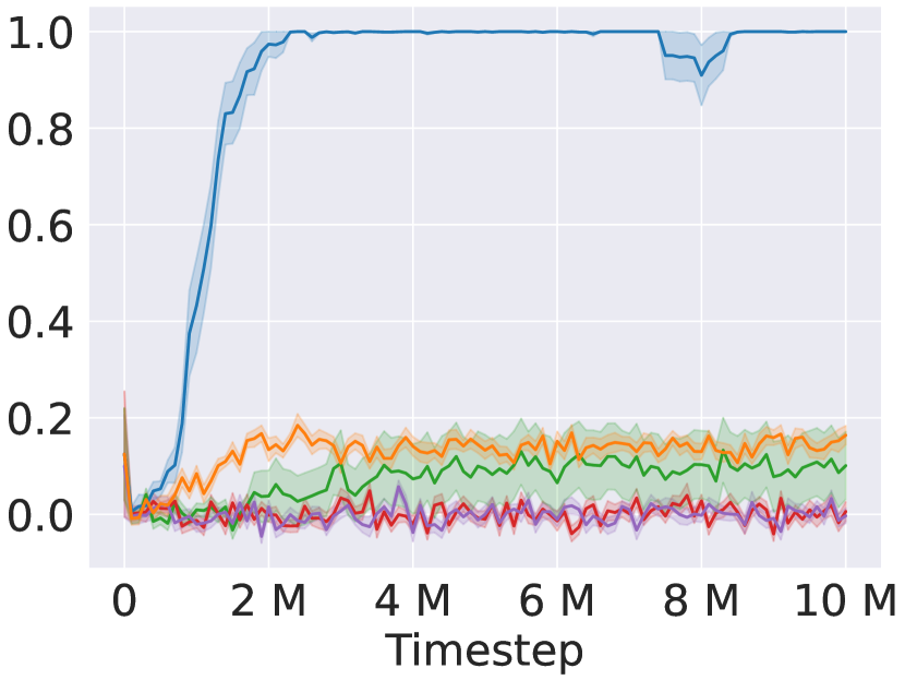
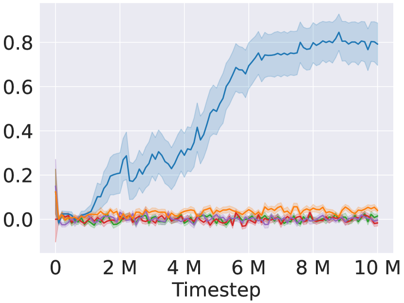
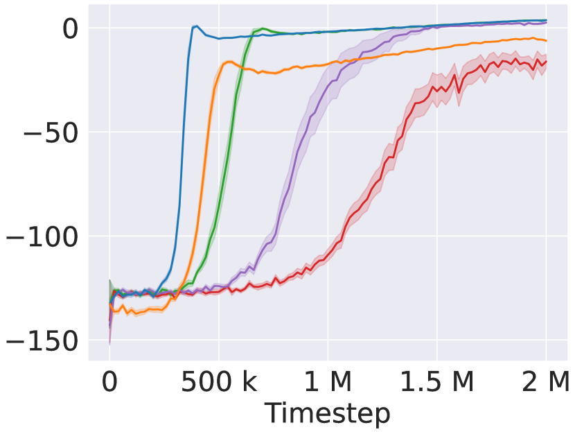
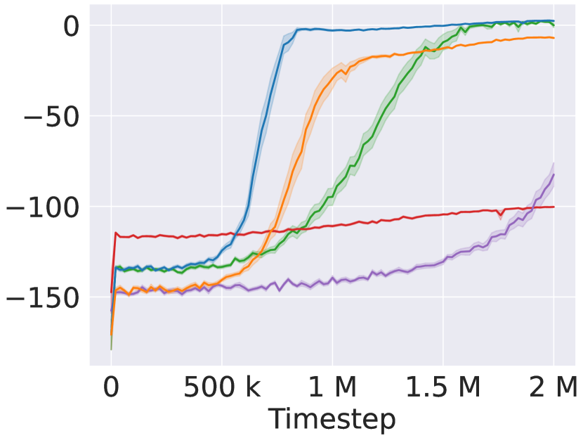
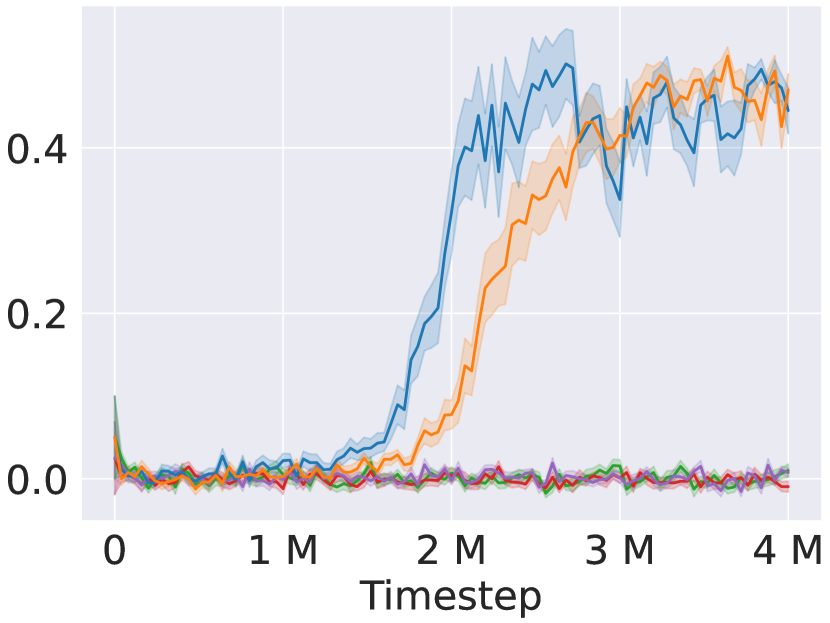
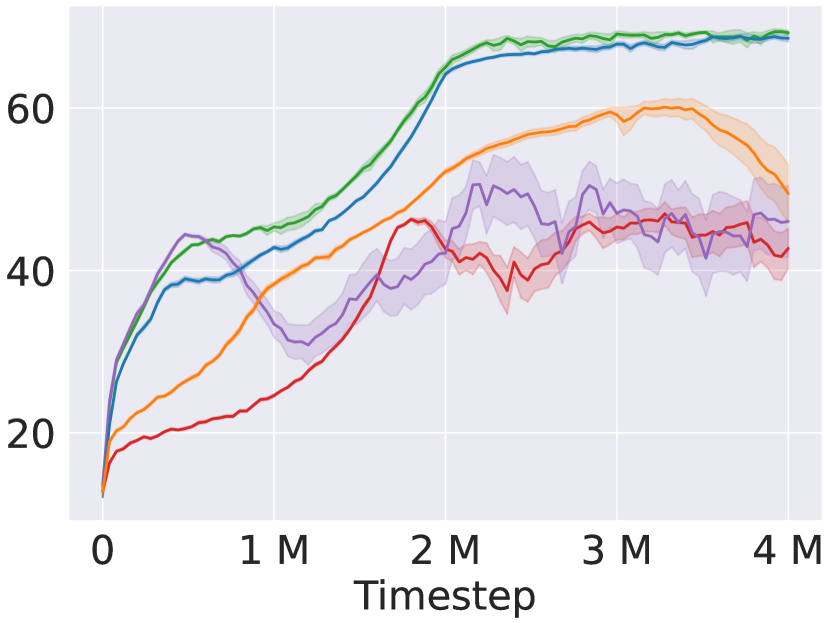
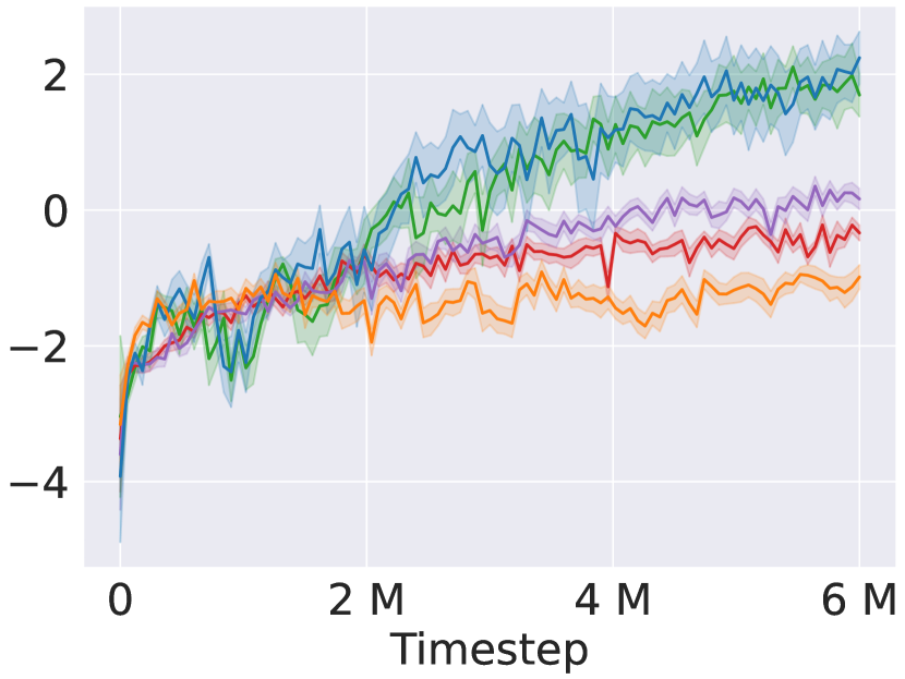
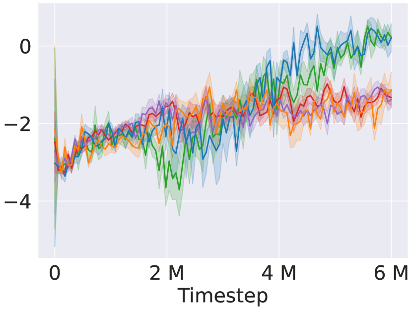
We compare the learning performances of five actor-critic variants. A2C, A2C-asym-s, and A2C-asym-hs are respectively (symmetric) A2C with history critic $\hat{V}{}(h)$, asymmetric A2C with state critic $\hat{V}{}(s)$, and asymmetric A2C with history-state critic $\hat{V}{}(h,s)$. To demonstrate that the environments feature significant partial observability, we include two “quasi-reactive” variants of (symmetric) A2C, meaning that they only receive a fixed number of recent actions and observations. A2C-react-2 and A2C-react-4 respectively receive the latest $2$ and $4$ actions and observations. We evaluate on $8$ navigation tasks which require different forms of information gathering and memorization: Heaven-Hell-3 and Heaven-Hell-4 Bonet (1998); Baisero (2019), Shopping-5 and Shopping-6 Baisero (2019), Car-Flag Nguyen (2021), Cleaner Jiang and Amato (2021), and Memory-Four-Rooms-7x7 and Memory-Four-Rooms-9x9 Baisero and Katt (2021); for details, see appendix Baisero and Amato (2022).

Each method is trained and evaluated using the same code (see Algorithm 1). Model architectures vary by environment; for more details, see Appendix D. For each method, we perform a grid-search over hyper-parameters of interest and select the hyper-parameter combination which leads to the best performance (prioritizing learning stability over convergence speed if needed); for more details, see appendix Baisero and Amato (2022). Each combination of hyper-parameters is evaluated over $20$ independent runs to guarantee statistical significance.

6.1. Results and Discussion

We show two relevant results from our evaluation: (a) in Figure 3, the empirical learning curve statistics, and (b) in Figure 4, how critic values change during training for important history-state pairs.

6.1.1. Learning Curves

We first note that the “quasi-reactive” baselines perform poorly in most domains, demonstrating that these control problems feature non-trivial partial observability which requires information gathering strategies and/or memorization of the past. Even in Shopping-5, where A2C-react-4 eventually manages to reach the performance of other successful methods, its convergence speed is significantly slower (Figure 3(c)). On the other hand, the non-reactive A2C either performs much better, indicating that the additional memory is useful if not necessary (Figures 3(c), 3(d), 3(f), 3(g) and 3(h)), or it also fails, indicating that the task is still challenging even when the entire history is available, due to representation learning difficulties (Figures 3(a), 3(b) and 3(e)).

The A2C-asym-s baseline displays a variety of characteristics depending on the environment, mostly problematic. While A2C-asym-s managed to achieve competitive performance in Car-Flag (Figure 3(e)), in all other cases it either completely fails to perform the task (Figures 3(a), 3(b), 3(g) and 3(h)), or it slowly converges to a sub-optimal behavior (Figures 3(c) and 3(d)). Cleaner in particular demonstrates instability issues, causing the performance to collapse after a certain point (Figure 3(f)). We argue that the poor convergence performance and learning instability displayed by A2C-asym-s are two facets of the theoretical issues discussed in Section 4. Poor final performance may be easily explained by the history-aliasing issue whereby the state critic model $\hat{V}{}(s)$ may not be able to correctly evaluate a given history, while instability may be easily explained by the lack of a well-defined state value function $V^{\pi{}}(s)$ altogether.

In contrast, our proposed unbiased asymmetric variant A2C-asym-hs displays some of the best learning characteristics across all environments. In Cleaner, Memory-Four-Rooms-7x7, and Memory-Four-Rooms-9x9, its performance matches that of A2C (Figures 3(f), 3(g) and 3(h)), while in Car-Flag it matches that of A2C-asym-s (Figure 3(e)). In and of itself, this indicates that A2C-asym-hs is able to exploit whichever source of information (history or state) happens to be more suitable in practice to solve a given task. On top of that, A2C-asym-hs demonstrates strictly better final performance and/or convergence speed than both A2C and A2C-asym-s in Shopping-5 and Shopping-6 (Figures 3(c) and 3(d)), demonstrating that it is not only able to use the best source of information, but also of combining both sources to achieve a higher best-of-both-worlds performance. This ability is pushed one step further and demonstrated in Heaven-Hell-3 and Heaven-Hell-4, where A2C-asym-hs is the only method capable of learning to solve the task at all (Figures 3(a) and 3(b)). These results strongly demonstrate the importance of exploiting asymmetric information in ways which are theoretically justified and sound, as done in our work.

6.1.2. Critic Values

(a) Heaven left, w/o priest visit.

(b) Heaven right, w/o priest visit.

(c) Heaven left, w/ priest visit.

(d) Heaven right, w/ priest visit.

Figure 4. Critic value statistics for $4$ key history-state pairs in Heaven-Hell-4, evaluated throughout training, with statistics computed over $20$ independent runs. Full description in text.

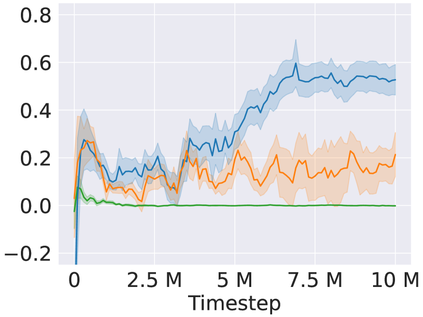
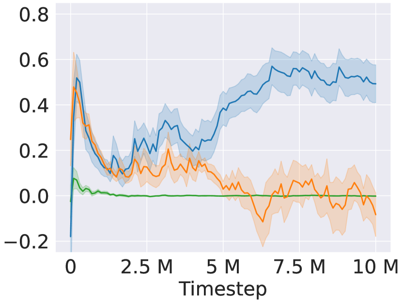
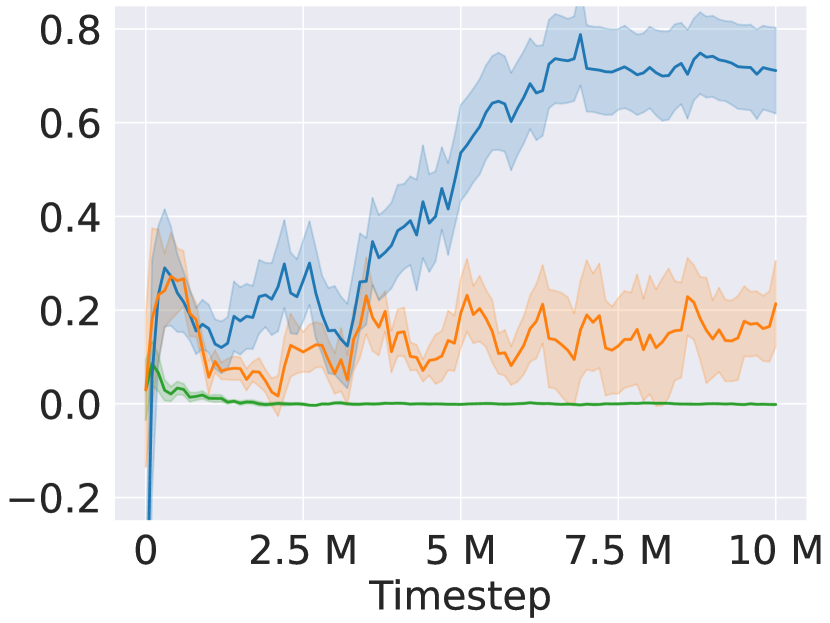
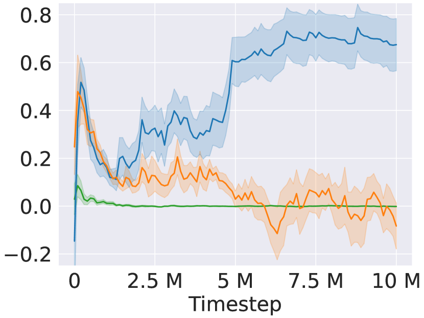
To further inspect the behavior of each critic, Figure 4 shows the evolution of critic values over the course of training for important history-state pairs in Heaven-Hell-4. We use $4$ deliberately chosen history-state pairs which are particularly important in this environment. In each case, the agent is located at the fork between heaven and hell, and the cases differ by the position of heaven (left or right) and whether the agent has previously performed the information-gathering sequence of actions necessary to know the position of heaven (by visiting the priest).

Unsurprisingly, we first note that critic values are correlated with the respective agent’s performance (Figure 3(b)). Beyond that, the critics show certain individual characteristics: namely, the critics which focus on a single aspect of the join history-state output the exact same values for different history-states. Although hard to see, the A2C critic $\hat{V}{}(h)$ outputs are identical in Figures 4(a) and 4(b), as those values are associated with the same histories (but not the same states). Similarly, the A2C-asym-s critic $\hat{V}{}(s)$ outputs are identical in Figures 4(a) and 4(c) and Figures 4(b) and 4(d) respectively, as those values are associated with the same states (but not the same histories). This confirms a straightforward truth: that the state critic $\hat{V}{}(s)$ is intrinsically unable to differentiave between values associated to different histories if they happen to be associated with the same state, which can be particularly detrimental in such information-gathering and memory dependent tasks. On the other hand, the A2C-asym-hs critic $\hat{V}{}(h,s)$ has the ability to output different values, as needed, for each of the four cases. Note, in particular, that the A2C-asym-hs critic is able to associate a higher reward to the agent if it has already performed the information-gathering actions (Figures 4(c) and 4(d)), compared to when it has not (Figures 4(a) and 4(b)), which helps the agent determine that the information-gathering actions are important and should be performed.

7. Conclusions

In partially observable control problems, the offline training/online execution framework offers the peculiar opportunity to access the system’s state during training, which otherwise remains latent during execution. Asymmetric methods trained offline can potentially exploit such privileged information to help train the agents to reach better performance and/or train more efficiently and using less data than before. While this idea has great potential, current state-of-the-art methods are motivated and driven by empirical results rather than theoretical analysis. In this work, we exposed fundamental theoretical issues with a standard variant of asymmetric actor-critic which made use of state critics $V^{\pi{}}(s)$, and proposed an unbiased asymmetric variant which makes use of history-state critics $V^{\pi{}}(h,s)$ and is the first of its kind to be analytically sound and theoretically justified. Although this represents a relatively simple change, its effects are profound, as demonstrated in both theoretical analysis and empirical results. Our evaluations confirm our analysis, and demonstrate both the issues with state-based critics and the benefits of history-state critics in environments which exhibit significant partial observability.

Although our evaluation only concerns A2C, the same concepts are easily extensible to other critic-based RL methods Silver et al. (2014); Lillicrap et al. (2015); Degris et al. (2012); Mnih et al. (2016). The potential for future work is varied. One possibility is to extend the theory of history-state value functions to optimal value functions $Q^{*}(h,s,a)$, and develop theoretically sound asymmetric variants of value-based deep RL methods such as DQN Mnih et al. (2013). Another possibility is to integrate asymmetric information with state-of-the-art maximum entropy value/critic-based methods such as soft Q-learning Haarnoja et al. (2017), and soft actor-critic Haarnoja et al. (2018). Finally, another venue for improvement is to extend our theory and approach to multi-agent methods, potentially bringing theoretical rigor and improved performance Foerster et al. (2018); Lowe et al. (2017); Li et al. (2019); Wang et al. (2020); Yang et al. (2018); Rashid et al. (2018); Mahajan et al. (2019); Rashid et al. (2020).

This research was funded by NSF award 1816382.

Appendix A Timed Value Functions

Section 4 shows that for a general POMDP and policy, the state value function $V^{\pi{}}(s)$ is not necessarily well-defined, in part due to issues caused by the lack of time information. Here, we consider addressing the primary issue by providing explicit time-index information via timed value functions, $V^{\pi{}}_{t}(s)$ and $Q^{\pi{}}_{t}(s,a)$, which represent the expected returns obtained when the agent finds itself in a state $s$ at time $t$,

$$V^{\pi{}}_{t}(s) =\sum_{a\in\mathcal{A}}\Pr(A_{t}=a\mid S_{t}=s)Q^{\pi{}}_{t}(s,a)\,,$$ (23)

$$Q^{\pi{}}_{t}(s,a) =R(s,a)+\gamma\operatorname{\mathbb{E}}_{s^{\prime}\mid s,a}\left[V^{\pi{}}_{t+1}(s^{\prime})\right]\,.$$ (24)

Once again, we analyze the state-dependent action distribution term to verify correctness, and expand it by integrating over histories; this time, we can use the explicit time-index information to integrate over histories of a given length only,

$$\Pr(A_{t}=a\mid S_{t}=s)=\sum_{h\in\mathcal{H}_{t}}\Pr(H_{t}=h\mid S_{t}=s)\pi{}(a;h)\,.$$ (25)

Because Equation 25 is now restricted to histories of a given length $t$, the probability term $\Pr(H_{t}=h\mid S_{t}=s)$ is well-defined, and in turn $\Pr(A_{t}=a\mid S_{t}=s)$ and $V^{\pi{}}_{t}(s)$ are likewise well-defined. Nevertheless, its utility for the purpose of asymmetric reinforcement learning remains unclear because (a) it is still not formally proven whether timed value functions are unbiased, i.e., whether $V^{\pi{}}_{t}(h)=\operatorname{\mathbb{E}}_{s\mid h}\left[V^{\pi{}}_{t}(s)\right]$, and (b) it is harder for timed value critics $\hat{V}{}(s,t)$ to generalize appropriately across the additional discrete input $t$.

Appendix B Additional Lemmas and Proofs

B.1. Differing Histories with Shared Beliefs

The main proof of Theorem 4.2 is based the commonly-known fact (which could be considered a lemma in its own right) that, in a generic POMDP, two different histories $h^{\prime}\neq h^{\prime\prime}$ may be associated with the same belief $b(h^{\prime})=b(h^{\prime\prime})$. This section contains some examples where this happens in some of the environments used in our evaluation. To better understand the environments, and therefore the following examples, see Appendix C.

Example 1

In Memory-Four-Rooms, consider the following histories:

• The agent turns left 4 times until it reaches the initial orientation.

• The agent turns right 4 times until it reaches the initial orientation.

• The agent turns any direction any number of times such that it ends up viewing all possible orientations, and finally reaches the initial orientation.

In each case, the agent has received the same amount of total information, just in a different order, which results in the same belief.

Example 2

In Heaven-Hell, consider any sequence of actions which does not reach an exit, does not result in visiting the priest, and ends with the agent occupying the same final position. At the end of any such sequence, the agent has full knowledge of its position, and no additional knowledge of the position of the door to heaven, i.e., all such sequences result in the same final belief.

Example 3

In Heaven-Hell, consider any sequence of actions which does not reach an exit, does result in visiting the priest, and ends with the agent occupying the same final position. At the end of any such sequence, the agent has full knowledge of both its position and the position of the door to heaven, i.e., all such sequences result in the same final belief.

B.2. Additional Proofs for Theorem 4.2

This section contains two additional proofs (one sketch and one formal) omitted from the main body of the document for the case of a reactive policy (Section 4.2). These two proofs complement the more general one of Theorem 4.2, and take into account the assumptions of a reactive policy and an observation function which depends only on the current state.

Proof (sketch) by contradiction.

First, we assume that $V^{\pi{}}(s)$ is unbiased and show that $Q^{\pi{}}(s,a)$ (as defined by Equation 10) is unbiased,

$$\operatorname{\mathbb{E}}_{s\mid h}\left[Q^{\pi{}}(s,a)\right] =\operatorname{\mathbb{E}}_{s\mid h}\left[\mathrm{R}(s,a)+\gamma\operatorname{\mathbb{E}}_{s^{\prime}\mid s,a}\left[V^{\pi{}}(s^{\prime})\right]\right]$$

$$=\operatorname{\mathbb{E}}_{s\mid h}\left[\mathrm{R}(s,a)\right]+\gamma\operatorname{\mathbb{E}}_{s\mid h}\left[\operatorname{\mathbb{E}}_{s^{\prime}\mid s,a}\left[V^{\pi{}}(s^{\prime})\right]\right]$$

$$=\operatorname{\mathbb{E}}_{s\mid h}\left[\mathrm{R}(s,a)\right]+\gamma\operatorname{\mathbb{E}}_{s^{\prime}\mid h,a}\left[V^{\pi{}}(s^{\prime})\right]$$

$$=\operatorname{\mathbb{E}}_{s\mid h}\left[\mathrm{R}(s,a)\right]+\gamma\operatorname{\mathbb{E}}_{o\mid h,a}\operatorname{\mathbb{E}}_{s^{\prime}\mid hao}\left[V^{\pi{}}(s^{\prime})\right]$$

$$=\mathrm{R}(h,a)+\gamma\operatorname{\mathbb{E}}_{o\mid h,a}\left[V^{\pi{}}(hao)\right]$$

$$=Q^{\pi{}}(h,a)\,.$$ (26)

Next, we show that even if $Q^{\pi{}}(s,a)$ is unbiased, $V^{\pi{}}(s)$ (as defined by Equation 9) is biased, which contradicts the original assumption. To do that, we expand the expected state value function $\operatorname{\mathbb{E}}_{s\mid h}\left[V^{\pi{}}(s)\right]$ and the history value function $V^{\pi{}}(h)$, and show that there is a concrete difference between them:

$$\operatorname{\mathbb{E}}_{s\mid h}\left[V^{\pi{}}(s)\right] =\operatorname{\mathbb{E}}_{s\mid h}\left[\sum_{a\in\mathcal{A}}\Pr(a\mid s)Q^{\pi{}}(s,a)\right]$$

$$=\operatorname{\mathbb{E}}_{s\mid h}\left[\sum_{a\in\mathcal{A}}\operatorname{\mathbb{E}}_{o\mid s}\left[\pi(a;o)\right]Q^{\pi{}}(s,a)\right]\,,$$ (27)

$$V^{\pi{}}(h) =\sum_{a\in\mathcal{A}}\pi(a;o_{h})Q^{\pi{}}(h,a)$$

$$=\sum_{a\in\mathcal{A}}\pi(a;o_{h})\operatorname{\mathbb{E}}_{s\mid h}\left[Q^{\pi{}}(s,a)\right]$$

$$=\operatorname{\mathbb{E}}_{s\mid h}\left[\sum_{a\in\mathcal{A}}\operatorname{\mathbb{E}}_{o\mid s}\left[\pi(a;o_{h})\right]Q^{\pi{}}(s,a)\right]\,.$$ (28)

Equations 27 and 28 differ in terms of which observation is used by the policy; in Equation 27, an observation $o$ inferred from a state $s$ inferred from the history $h$ is used, while in Equation 28 the final observation $o_{h}$ of the history $h$ is used. These two observations $o$ and $o_{h}$ are not generally the same, and the respective expectations are similarly not generally the same. The nested expectation in Equation 27 can be interpreted as a lossy round-trip inference from history to state and from state back to observation $h\to s\to o$. Although histories and states tend to be somewhat correlated, both state aliasing and history aliasing make the roundtip conversion imperfect, causing a mismatch between the expected state value function $\operatorname{\mathbb{E}}_{s\mid h}\left[V^{\pi{}}(s)\right]$ and the history value function $V^{\pi{}}(h)$ in the general control case of a general POMDP. ∎

Proof by example.

This is a proof by example (with a proof by contradiction element). We will define the good/bad POMDP and, for a specific policy and history, first calculate $\operatorname{\mathbb{E}}_{s\mid h}\left[V^{\pi{}}(s)\right]$ exactly, and then $V^{\pi{}}(h)$ using bootstrapping (while also assuming $V^{\pi{}}(hao)=\operatorname{\mathbb{E}}_{s^{\prime}\mid hao}\left[V^{\pi{}}(s^{\prime})\right]$). We show that the two values are numerically different.

In the good/bad POMDP, $\mathcal{S}=\{\texttt{GOOD},\texttt{BAD}\},\mathcal{A}=\{\texttt{GOOD},\texttt{BAD}\}$, $\mathcal{O}=\{\texttt{GOOD},\texttt{BAD}\}$; At times, we will use the shorthands G and B. The initial state distribution is uniform, and each state deterministically transitions into itself. The GOOD state always emits the GOOD observation, while the BAD state emits a random observation. Consider the reward function such that $R(s,a)=\operatorname{\mathbb{I}}\left[a=\texttt{GOOD}\right]$, i.e., the agent receives a reward whenever it choses the GOOD action. We will denote a history as the concatenation of alternating observations and actions, starting with an observation. To keep the notation compact, we will occasionally use symbols G and B to represent GOOD and BAD states, observations and actions. Consider a deterministic policy $\pi(a;h)=\operatorname{\mathbb{I}}\left[a=o_{h}\right]$ which returns the action corresponding to the last observation. Note that this POMDP and this policy satisfy the requirements to guarantee that $V^{\pi{}}(s)$ is well defined.

Next, we calculate the state values $V^{\pi{}}(s)$. The GOOD state always emits the GOOD observation, so the agent will always choose the GOOD action and receive a reward of $1$, then the state will always transition into itself,

$$V^{\pi{}}(s=\texttt{GOOD}) =1+\gamma V^{\pi{}}(s=\texttt{GOOD})$$

$$=\frac{1}{1-\gamma}\,.$$ (29)

On the other hand, the BAD state will only emit the GOOD observation half of the times, so the agent will only choose the GOOD action and receive a reward of $1$ half of the times, then the state will always transition into itself,

$$V^{\pi{}}(s=\texttt{BAD}) =\frac{1}{2}+\gamma V^{\pi{}}(s=\texttt{BAD})$$

$$=\frac{1}{2(1-\gamma)}\,.$$ (30)

Next, we consider the history $h=\texttt{G}$ after a single initial GOOD observation, and calculate the history value $V^{\pi{}}(h)$. Before proceeding, we need to calculate a few intermediate quantities, such as the belief-distribution:

$$\Pr(s=\texttt{G}\mid h=\texttt{G}) \propto\Pr(h=\texttt{G}\mid s=\texttt{G})\Pr(s=\texttt{G})$$

$$=1\frac{1}{2}$$

$$=\frac{1}{2}\,,$$ (31)

$$\Pr(s=\texttt{B}\mid h=\texttt{G}) \propto\Pr(h=\texttt{G}\mid s=\texttt{B})\Pr(s=\texttt{B})$$

$$=\frac{1}{2}\frac{1}{2}$$

$$=\frac{1}{4}\,,$$ (32)

therefore

$$\Pr(s=\texttt{G}\mid h=\texttt{G}) =\frac{2}{3}\,,$$ (33)

$$\Pr(s=\texttt{B}\mid h=\texttt{G}) =\frac{1}{3}\,.$$ (34)

We also calculate the belief-state distribution after two other histories. First $h=\texttt{G}\texttt{G}\texttt{G}$,

$$\Pr(s=\texttt{G}\mid h=\texttt{G}\texttt{G}\texttt{G}) \propto\Pr(h=\texttt{G}\texttt{G}\texttt{G}\mid s=\texttt{G})\Pr(s=\texttt{G})$$

$$=1\frac{1}{2}$$

$$=\frac{1}{2}\,,$$ (35)

$$\Pr(s=\texttt{B}\mid h=\texttt{G}\texttt{G}\texttt{G}) \propto\Pr(h=\texttt{G}\texttt{G}\texttt{G}\mid s=\texttt{B})\Pr(s=\texttt{B})$$

$$=\frac{1}{4}\frac{1}{2}$$

$$=\frac{1}{8}\,,$$ (36)

therefore

$$\Pr(s=\texttt{G}\mid h=\texttt{G}\texttt{G}\texttt{G}) =\frac{4}{5}\,,$$ (37)

$$\Pr(s=\texttt{B}\mid h=\texttt{G}\texttt{G}\texttt{G}) =\frac{1}{5}\,.$$ (38)

Then $h=\texttt{G}\texttt{G}\texttt{B}$,

$$\Pr(s=\texttt{G}\mid h=\texttt{G}\texttt{G}\texttt{B}) \propto\Pr(h=\texttt{G}\texttt{G}\texttt{B}\mid s=\texttt{G})\Pr(s=\texttt{G})$$

$$=0\frac{1}{2}$$

$$=0\,,$$ (39)

$$\Pr(s=\texttt{B}\mid h=\texttt{G}\texttt{G}\texttt{B}) \propto\Pr(h=\texttt{G}\texttt{G}\texttt{B}\mid s=\texttt{B})\Pr(s=\texttt{B})$$

$$=\frac{1}{4}\frac{1}{2}$$

$$=\frac{1}{8}\,,$$ (40)

therefore

$$\Pr(s=\texttt{G}\mid h=\texttt{G}\texttt{G}\texttt{B}) =0\,,$$ (41)

$$\Pr(s=\texttt{B}\mid h=\texttt{G}\texttt{G}\texttt{B}) =1\,.$$ (42)

We also need to calculate the observation emission probabilities,

$$\Pr(o=\texttt{G}\mid h=\texttt{G},a=\texttt{G}) =\Pr(s=\texttt{G}\mid h=\texttt{G})\Pr(o=\texttt{G}\mid s=\texttt{G})$$

$$\hphantom{{}={}}+\Pr(s=\texttt{B}\mid h=\texttt{G})\Pr(o=\texttt{G}\mid s=\texttt{B})$$

$$=\frac{2}{3}1+\frac{1}{3}\frac{1}{2}$$

$$=\frac{5}{6}\,,$$ (43)

$$\Pr(o=\texttt{B}\mid h=\texttt{G},a=\texttt{G}) =\Pr(s=\texttt{G}\mid h=\texttt{G})\Pr(o=\texttt{B}\mid s=\texttt{G})$$

$$\hphantom{{}={}}+\Pr(s=\texttt{B}\mid h=\texttt{G})\Pr(o=\texttt{B}\mid s=\texttt{B})$$

$$=\frac{2}{3}0+\frac{1}{3}\frac{1}{2}$$

$$=\frac{1}{6}\,.$$ (44)

Next, we calculate $V^{\pi{}}(h=\texttt{G})$ under the assumption that the equality holds,

$$V^{\pi{}}(h=\texttt{G}) =\operatorname{\mathbb{E}}_{s\mid h=\texttt{G}}\left[V^{\pi{}}(s)\right]$$

$$=\Pr(s=\texttt{G}\mid h=\texttt{G})V^{\pi{}}(s=\texttt{G})+\Pr(s=\texttt{B}\mid h=\texttt{G})V^{\pi{}}(s=\texttt{B})$$

$$=\frac{2}{3}\frac{1}{1-\gamma}+\frac{1}{3}\frac{1}{2(1-\gamma)}$$

$$=\frac{5}{6(1-\gamma)}\,.$$ (45)

We can also apply the equality to other histories,

$$V^{\pi{}}(h=\texttt{G}\texttt{G}\texttt{G}) =\operatorname{\mathbb{E}}_{s\mid h=\texttt{G}\texttt{G}\texttt{G}}\left[V^{\pi{}}(s)\right]$$

$$=\Pr(s=\texttt{G}\mid h=\texttt{G}\texttt{G}\texttt{G})V^{\pi{}}(s=\texttt{G})+\Pr(s=\texttt{B}\mid h=\texttt{G}\texttt{G}\texttt{G})V^{\pi{}}(s=\texttt{B})$$

$$=\frac{4}{5}\frac{1}{1-\gamma}+\frac{1}{5}\frac{1}{2(1-\gamma)}$$

$$=\frac{9}{10(1-\gamma)}\,,$$ (46)

$$V^{\pi{}}(h=\texttt{G}\texttt{G}\texttt{B}) =\operatorname{\mathbb{E}}_{s\mid h=\texttt{G}\texttt{G}\texttt{B}}\left[V^{\pi{}}(s)\right]$$

$$=\Pr(s=\texttt{G}\mid h=\texttt{G}\texttt{G}\texttt{B})V^{\pi{}}(s=\texttt{G})+\Pr(s=\texttt{B}\mid h=\texttt{G}\texttt{G}\texttt{B})V^{\pi{}}(s=\texttt{B})$$

$$=0\frac{1}{1-\gamma}+1\frac{1}{2(1-\gamma)}$$

$$=\frac{1}{2(1-\gamma)}\,.$$ (47)

Next, we calculate $V^{\pi{}}(h=\texttt{G})$, this time by bootstrapping first, and then using the equality. Note that with the given history $h=\texttt{G}$, the agent will choose action $a=\texttt{GOOD}$. Then,

$$V^{\pi{}}(h=\texttt{G}) =R(h=\texttt{G},a=\texttt{G})+\gamma\operatorname{\mathbb{E}}_{o\mid h=\texttt{G},a=\texttt{G}}\left[V^{\pi{}}(hao=\texttt{G}\texttt{G}o)\right]$$

$$=1+\gamma\left(\begin{aligned} \Pr(o=\texttt{G}\mid h=\texttt{G},a=\texttt{G})V^{\pi{}}(hao=\texttt{G}\texttt{G}\texttt{G})\\ +\Pr(o=\texttt{B}\mid h=\texttt{G},a=\texttt{G})V^{\pi{}}(hao=\texttt{G}\texttt{G}\texttt{B})\end{aligned}\right)$$

$$=1+\gamma\frac{5}{6}\frac{9}{10(1-\gamma)}+\gamma\frac{1}{6}\frac{1}{2(1-\gamma)}$$

$$=\frac{60-60\gamma}{60(1-\gamma)}+\frac{45\gamma}{60(1-\gamma)}+\frac{5\gamma}{60(1-\gamma)}$$

$$=\frac{60-10\gamma}{60(1-\gamma)}$$

$$=\frac{6-\gamma}{6(1-\gamma)}\,.$$ (48)

The values from Equations 45 and 48 contradict each other, therefore, for this POMDP, policy, and history, $V^{\pi{}}(h)\neq\operatorname{\mathbb{E}}_{s\mid h}\left[V^{\pi{}}(s)\right]$. ∎

Appendix C Environments

In this section, we present a detailed description of each control problem. While all problems are controlled by categorical actions, they can be split into three groups based on the types of state and observation representations provided to the agent:

• Heaven-Hell-3, Heaven-Hell-4, Shopping-5, and Shopping-6 are categorical POMDPs,

• Car-Flag and Cleaner are feature-vector POMDPs,

• Memory-Four-Rooms-7x7 and Memory-Four-Rooms-9x9 are gridverse POMDPs.

C.1. Categorical POMDPs

(a) Heaven-Hell-3

(b) Heaven-Hell-4

Figure 5. Layout of the Heaven-Hell environments.

(a) Shopping-5

(b) Shopping-6

Figure 6. Layout of the Shopping environments.

The implementation of the categorical POMDPs (and their POMDP files) can be found in Baisero (2019). In the categorical POMDPs, states, actions and observations are all encoded by categorical indices which have no inherent metric, and which are intrinsically equally (dis)similar to each other. While it is not possible to generalize across states and observations via feature extraction, the primary challenge in these POMDPs is that of generalizing across different histories. Because the categorical POMDPs are finite, their state, action and observation spaces have well-defined sizes, shown in Table 1; note, however, that the size of the state space is not a significant measure of the complexity of partially observable tasks, while the time required to solve the task (i.e., history length) is a more relevant measure. While these types of POMDPs often do not look as impressive as others, due to the unimpressive categorical representations, they pose unique learning challenges which tend to focus on the core of decision making, rather than mere feature extraction.

Table 1. Categorical environment properties.

Domain	$|\mathcal{S}|$	$|\mathcal{A}|$	$|\mathcal{O}|$	$\gamma$
Shopping-5	625	6	50	0.99
Shopping-6	1296	6	72	0.99
Heaven-Hell-3	28	4	15	0.99
Heaven-Hell-4	36	4	19	0.99

C.1.1. Heaven-Hell

In Heaven-Hell Bonet (1998), the agent navigates a corridor-like gridworld composed of a fork and $3$ dead-ends. Two dead-ends are exits which lead to heaven or hell, although the agent does not know which is which, while the third dead-end leads to a priest who can help the agent identify the heaven exit. Figure 5 depicts the gridworlds encoded by Heaven-Hell-3 and Heaven-Hell-4.

States and Observations

States encode the position of the agent and the position of the exit to heaven. Observations encode the position of the agent or the position of the exit to heaven.

Actions

Each time-step, the agent must choose an action from the set { NORTH, SOUTH, EAST, WEST }. If the agent is at the priest, it observes heaven’s location, otherwise it observes its own position. To solve the task, the agent needs to navigate to the priest, then back to the fork, and on to heaven.

Rewards

The agent receives a sparse reward signal composed of:

• a reward of $1.0$ for exiting to heaven; and

• a reward of $-1.0$ for exiting to hell.

C.1.2. Shopping

Shopping simulates an agent going to a shop to buy an item it forgot. The agent navigates a $5\times 5$ or $6\times 6$ gridworld trying to locate and select a randomly positioned item. The agent’s position is fully observable, while the item’s position is only observed when queried. Figure 6 depicts the gridworlds encoded by Shopping-5 and Shopping-6.

States and Observations

States encode the position of the agent and the position of the item in a single integer. Observations encode the position of the agent or the position of the item in a single integer.

Actions

Each time-step, the agent must choose an action from the set { LEFT, RIGHT, UP, DOWN, QUERY, BUY }. If the agent chooses the QUERY action, it observes the item’s position, otherwise it observes its own position. To solve the task optimally, the agents needs to query the item’s position and remember it, navigate to it, and then buy it.

Rewards

The agent receives the following reward signal:

• a reward of $-1.0$ for moving;

• a reward of $-2.0$ for performing a QUERY action;

• a reward of $-5.0$ for performing a BUY action in the wrong cell; and

• a reward of $10.0$ for performing a BUY action in the correct cell.

C.2. Feature-Vector POMDPs

In the feature-vector POMDPs, states and observations are provided as concise feature vectors where each dimension represents a particular aspect of the state/observation, e.g., in navigation tasks, one dimension could represent the horizontal position of the agent. Typically, the observation feature vectors are obtained by dropping selected dimensions from the state feature vector.

(a) Car-Flag

(b) Cleaner

Figure 7. Screenshots of the Car-Flag and Cleaner environments.

C.2.1. Car-Flag

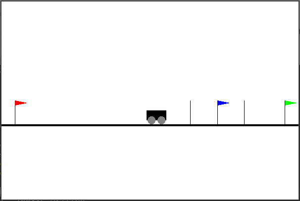
The implementation of Car-Flag can be found in Nguyen (2021). The agent uses force-control on a car moving along a 1-dimensional axis. On opposite extremes are a good and a bad flags which, if reached, respectively end the episode positive and negatively. Along the line, a third info flag appears, which allows the agent to observe the position of the good flag. Figure 7(a) depicts Car-Flag. This setup is similar to Heaven-Hell, although with force-control and the position of the info flag being significant differences.

States and Observations

States and observations are both three-dimensional vectors. In the states features, the first two dimensions respectively contain the agent position and velocity, while the third dimension contains the position of the good flag. The observations are analogous, with the difference that the third dimension is masked out (set to zero) when the agent is not within range of the info flag.

Actions

Each time-step, the agent must choose how to accelerate the car using one of $7$ possible actions representing { LEFT_HIGH, LEFT_MEDIUM, LEFT_LOW, NONE, RIGHT_HIGH, RIGHT_MEDIUM, RIGHT_LOW }.

Rewards

The agent receives a sparse reward signal composed of:

• a reward of $1.0$ for reaching the good flag; and

• a reward of $-1.0$ for reaching the bad flag.

C.2.2. Cleaner

Cleaner Jiang and Amato (2021) is originally a 2-agent environment; however, for the purpose of our evaluation, we frame it as a single-agent control problem via fully centralized training and execution. As a result, the problem’s actions and observations are obstained via Cartesian product of the respective actions and observations of each separate agent. In Cleaner, two robots must cover the entire area of a $13\times 13$ maze-like environment in order to clean it. The task is complete when every cell in the grid has been visited by at least one agent. The environment is depicted in Figure 7(b).

States and Observations

The state is provided as a $13\times 13\times 5$ binary tensor, indicating, for each position in the grid, whether it contains a wall, a dirty cell, a clean cell, the first agent, or the second agent. Each agent’s observation is given as a $3\times 3\times 3$ binary tensor encoding the $3\times 3$ area surrounding the agent.

Actions

Each agent can move in one of the four directions using actions { LEFT, RIGHT, UP, DOWN }. In the centralized control version of this problem, this results in $16$ possible actions.

Rewards

In each time-step, a unit reward is given for each new tile cleaned, resulting in three possible rewards: $0.0$, $1.0$, and $2.0$.

C.3. Gridverse POMDPs

(a) State.

(b) Observation.

Figure 8. Memory-Four-Rooms-7x7. Note that the states and observations are not provided as images to the agent; these are visualizations for human understanding.

(a) State.

(b) Observation.

Figure 9. Memory-Four-Rooms-9x9. Note that the states and observations are not provided as images to the agent; these are visualizations for human understanding.

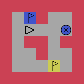
The implementation of the gridverse POMDPS can be found in Baisero and Katt (2021). In the gridverse POMDPs, actions are still encoded by categorical indices, while states and observations are encoded as structures which do have an inherent similarity metric; they are split into different components, some of which are only available in the state, or which take a different form in the observation:

• A grid component: a $3\times H\times W$ volume of categorical indices which encode cell type, cell color, and cell status. The observation grid component is a slice of the corresponding state grid component made to match the agent’s perspective: it is rotated to be a first-person view, as shown in Figures 8(b) and 9(b), and cells hidden behind walls, if within the observation slice, are occluded.

• An agent_id_grid component: a $H\times W$ binary matrix which encode the agent’s position. This is only available in the state.

• An agent component: a $3$-dimensional array of categorical indices representing the agent position and orientation. The position and orientations in the state agent component are absolute, while those in the observation component are relative to the agent’s perspective—they are essentially constant, and not necessary for control.

• An item component: a $3$-dimensional array of categorical indices representing the item held by the agent, if any. While some gridverse tasks do involve manipulation of items, the ones used in our evaluation do not, and this component could potentially be ignored.

C.3.1. Memory-Four-Rooms

The agent navigates a $7\times 7$ or $9\times 9$ gridworld split into four rooms; randomly positioned are a good exit, a bad exit, and a beacon with the same color as the good exit. To solve the task, the agent must find the beacon, observe and remember its color, and use it to identify and reach the good exit which has the same color. The positions of the agent, the exits, and the beacon, as well as the colors of the exits and beacons are randomly sampled such that each episode is unique. Figures 8 and 9 shows state and observation frames respectively taken from instances of Memory-Four-Rooms-7x7 and Memory-Four-Rooms-9x9.

States and Observations

For Memory-Four-Rooms-7x7, the state grid component is a $3\times 7\times 7$ volume, while the observation grid component is a $3\times 2\times 3$ volume representing a $2\times 3$ view of the agent surroundings. For Memory-Four-Rooms-9x9, the state grid component is a $3\times 9\times 9$ volume.

Actions

Each time-step, the agent must choose an action from the set { MOVE_FORWARD, MOVE_BACKWARD, MOVE_LEFT, MOVE_RIGHT, TURN_LEFT, TURN_RIGHT, PICK_N_DROP, ACTUATE }. The MOVE_* actions result in a movement depending on the agent’s orientation, while the TURN_* allows the agent to change its orientation. With the PICK_N_DROP action, the agent can pick and/or drop the key from/to the cell in front, while with the ACTUATE action, the agent can open and/or close doors. Memory-Four-Rooms-7x7 and Memory-Four-Rooms-9x9have no doors or pickable items, therefore the last two actions have no effect.

Rewards

The agent receives a dense reward signal composed as the sum of the following terms:

• a living reward of $-0.05$ for every time-step;

• a reward of $5.0$ for reaching the good exit;

• a reward of $-5.0$ for reaching the bad exit.

Appendix D Model Architectures

(a) State, action, and observation representation models used for flat POMDPs.

(b) State, action, and observation representation models used for gridverse POMDPs.

(c) A2C architecture. Separate components are used for policy and critic models. For the categorical and gridverse environments, state, action, and observation representations $\phi(s)$, $\phi(a)$, and $\phi(o)$ are shown in Figure 10(a) and Figure 10(b). For the feature-vector environments, states and observation representations $\phi(s)$ and $\phi(o)$ are directly provided by the environment directly, while action representations $\phi(a)$ are implemented as embeddings. Dotted lines are present or omitted depending on whether a history critic $\hat{V}{}(h)$, state critic $\hat{V}{}(s)$, or history-state critic $\hat{V}{}(h,s)$ is being modeled.

Figure 10.

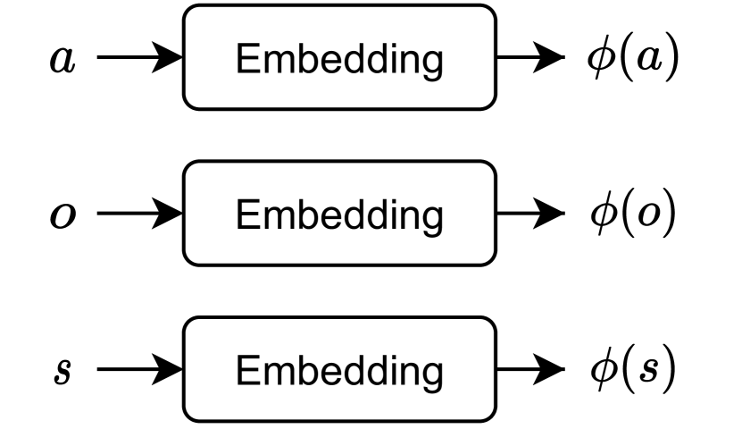
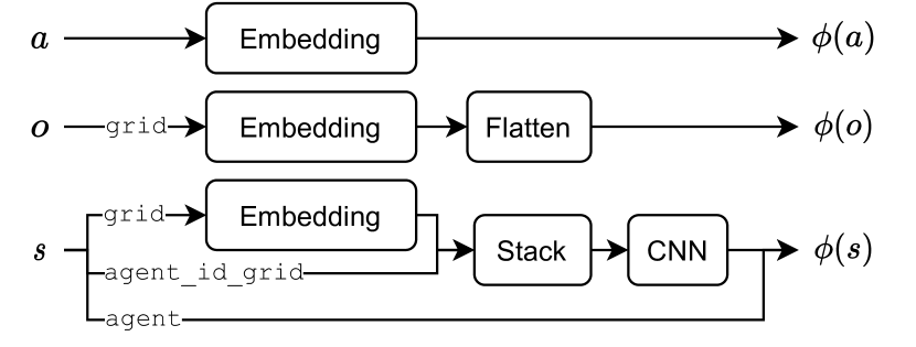
In this section, we describe the architectures used by the policy and critic models for each environment, also shown in Figure 10. The general architecture will be similar for all domains; however there will some differences to accommodate the different state and observation representations provided by each environment.

General Architecture

These components are shown in Figure 10(c). Policy and critic models share part of the architecture, but not the associated parameters. Concatenated action and observation features form the input to a $128$-dimensional single-layer gated recurrent unit (GRU) Cho et al. (2014), which acts as a history representation $\phi(h)$. The policy and value NN components vary in each environment.

Categorical POMDPs

The action, state, and observation feature components are shown in Figure 10(a). Because categorical POMDPs provide states, actions and observations as categorical indices, we use $64$-dimensional embedding models to represent each of them. The policy and value NN components are each $2$-layer feedforward models with $512$ and $256$ nodes with ReLU non-linearities.

Feature-Vector POMDPs

The action featues are one-hot encodings of the respective categorical indices. Because the states and observations provided by the environments already come in a simple and flat feature representation, we do not process them further. The policy and value NN components are each $2$-layer feedforward models with $512$ and $256$ nodes with ReLU non-linearities.

Gridverse POMDPs

These feature extraction components are shown in Figure 10(b). Because gridverse POMDPs provide actions as categorical indices, we use $1$-dimensional embedding models to represent them, i.e., we focus on the state and observation representations as they contain the most relevant information. On the other hand, states and observations are provided in the format described in Section C.3. The $3\times 2\times 3$ observations are first processed using an $8$-dimensional embedding layer, and then flattened, which produces a $144$-dimensional observation feature $\phi(o)$. The states contain relevant information in different forms, and require a more complex model. The grid component is processed using an embedding layer, which is then stacked with the agent_id_grid component, and processed by a $3$-layer convolutional network. The output of the convolutional layers is concatenated with the agent components, to form the overall state feature $\phi(s)$. The policy and value NN components are each single-layer feedforward models with $512$ nodes with ReLU non-linearities.

Appendix E Hyperparameters and Grid Search

For each environment and method, we perform a separate hyper-parameter grid search to find the respective best training performance possible. In each case, the grid search is performed over the following hyper-parameters and ranges of values:

1. the actor learning rate $\alpha_{\pi{}}$, searched over values 0.0001, 0.0003, and 0.001,

2. the critic learning rate $\alpha_{\hat{V}{}}$, searched over values 0.0001, 0.0003, and 0.001,

3. the initial negative-entropy weight $\lambda_{0}$, searched over environment-dependent values:

   Heaven-Hell-3:

   0.01, 0.03, 0.1, 0.3, 1.0.

   Heaven-Hell-4:

   0.01, 0.03, 0.1, 0.3, 1.0.

   Shopping-5:

   0.3, 1.0, 3.0, 10.0, 30.0.

   Shopping-6:

   0.3, 1.0, 3.0, 10.0, 30.0.

   Car-Flag:

   0.03, 0.1, 0.3, 1.0, 3.0.

   Cleaner:

   0.03, 0.1, 0.3, 1.0, 3.0.

   Memory-Four-Rooms-7x7:

   0.01, 0.03, 0.1, 0.3, 1.0.

   Memory-Four-Rooms-9x9:

   0.01, 0.03, 0.1, 0.3, 1.0.

In total, a full grid search over these hyper-parameters amounts to $3\cdot 3\cdot 5=45$ different hyper-parameter possibilities for each environment and method. Factoring in the $20$ independent runs, the $5$ methods, and $8$ environments, this adds up to $45\cdot 20\cdot 5\cdot 8=36$k separate runs. The optimal hyperparameters for each case are shown in Table 2. Other relevant hyper-parameters are set as follows:

• The negative-entropy weight decays linearly over the course of $2$M timesteps to a final value equal one tenth of the initial one, $\frac{\lambda_{0}}{10}$.

• The number of episodes sampled per gradient step ($E$ in Algorithm 1) is set to $2$.

• Episodes are automatically terminated if they do not end after $100$ timesteps.

• A frozen target model is used to stabilize the training of critics, with the target model parameters being updated every $10$k timesteps.

Table 2. Hyperparameter grid search results.

Domain	Method	$\alpha_{\pi{}}$	$\alpha_{\hat{V}{}}$	$\lambda_{0}$
Heaven-Hell-3	A2C-asym-hs	0.001	0.001	0.1
	A2C-asym-s	0.001	0.001	1.0
	A2C	0.001	0.001	0.1
	A2C-react-2	0.001	0.0003	1.0
	A2C-react-4	0.001	0.0003	1.0
Heaven-Hell-4	A2C-asym-hs	0.001	0.001	0.1
	A2C-asym-s	0.001	0.001	0.1
	A2C	0.001	0.0003	0.3
	A2C-react-2	0.001	0.0003	0.3
	A2C-react-4	0.001	0.0003	0.3
Shopping-5	A2C-asym-hs	0.001	0.0003	3.0
	A2C-asym-s	0.001	0.001	10.0
	A2C	0.001	0.0003	3.0
	A2C-react-2	0.001	0.001	3.0
	A2C-react-4	0.001	0.001	3.0
Shopping-6	A2C-asym-hs	0.001	0.0003	3.0
	A2C-asym-s	0.001	0.001	10.0
	A2C	0.001	0.0003	3.0
	A2C-react-2	0.001	0.001	1.0
	A2C-react-4	0.001	0.0003	10.0
Car-Flag	A2C-asym-hs	0.001	0.001	0.03
	A2C-asym-s	0.001	0.001	0.03
	A2C	0.001	0.001	0.03
	A2C-react-2	0.001	0.001	0.03
	A2C-react-4	0.001	0.001	0.03
Cleaner	A2C-asym-hs	0.001	0.001	1.0
	A2C-asym-s	0.001	0.001	1.0
	A2C	0.001	0.001	1.0
	A2C-react-2	0.001	0.001	3.0
	A2C-react-4	0.001	0.001	1.0
Memory-Four-Rooms-7x7	A2C-asym-hs	0.0003	0.001	0.1
	A2C-asym-s	0.0003	0.001	0.01
	A2C	0.0003	0.0001	0.1
	A2C-react-2	0.001	0.001	0.3
	A2C-react-4	0.001	0.001	0.3
Memory-Four-Rooms-9x9	A2C-asym-hs	0.001	0.0003	0.3
	A2C-asym-s	0.001	0.0003	0.1
	A2C	0.001	0.0003	0.3
	A2C-react-2	0.001	0.001	0.1
	A2C-react-4	0.001	0.001	0.1

References

- (1)
- Baisero (2019) Andrea Baisero. 2019. gym-pomdps: Gym environments from POMDP files. https://github.com/abaisero/gym-pomdps.
- Baisero and Amato (2022) Andrea Baisero and Christopher Amato. 2022. Unbiased Asymmetric Reinforcement Learning under Partial Observability. arXiv:2105.11674 [cs.LG]
- Baisero and Katt (2021) Andrea Baisero and Sammie Katt. 2021. gym-gridverse: Gridworld domains for fully and partially observable reinforcement learning. https://github.com/abaisero/gym-gridverse.
- Bonet (1998) Blai Bonet. 1998. Solving large POMDPs using real time dynamic programming. In AAAI Fall Symposium on POMDPs.
- Bono et al. (2018) Guillaume Bono, Jilles Dibangoye, Laëtitia Matignon, Florian Pereyron, and Olivier Simonin. 2018. On the Study of Cooperative Multi-Agent Policy Gradient.
- Chen et al. (2020) Dian Chen, Brady Zhou, Vladlen Koltun, and Philipp Krähenbühl. 2020. Learning by cheating. In Conference on Robot Learning. PMLR, 66–75.
- Cho et al. (2014) Kyunghyun Cho, Bart Van Merriënboer, Dzmitry Bahdanau, and Yoshua Bengio. 2014. On the properties of neural machine translation: Encoder-decoder approaches. (2014). arXiv:1409.1259 [cs.CL]
- de Witt et al. (2021) Christian Schroeder de Witt, Bei Peng, Pierre-Alexandre Kamienny, Philip Torr, Wendelin Böhmer, and Shimon Whiteson. 2021. Deep Multi-Agent Reinforcement Learning for Decentralized Continuous Cooperative Control. (2021). arXiv:2003.06709 [cs.LG]
- Degris et al. (2012) Thomas Degris, Martha White, and Richard S. Sutton. 2012. Off-policy actor-critic. (2012). arXiv:1205.4839 [cs.LG]
- Foerster et al. (2018) Jakob Foerster, Gregory Farquhar, Triantafyllos Afouras, Nantas Nardelli, and Shimon Whiteson. 2018. Counterfactual multi-agent policy gradients. Proceedings of the AAAI Conference on Artificial Intelligence 32, 1 (2018).
- Greensmith et al. (2004) Evan Greensmith, Peter L. Bartlett, and Jonathan Baxter. 2004. Variance reduction techniques for gradient estimates in reinforcement learning. Journal of Machine Learning Research 5 (2004), 1471–1530.
- Haarnoja et al. (2017) Tuomas Haarnoja, Haoran Tang, Pieter Abbeel, and Sergey Levine. 2017. Reinforcement learning with deep energy-based policies. In International Conference on Machine Learning, Vol. 70. PMLR.
- Haarnoja et al. (2018) Tuomas Haarnoja, Aurick Zhou, Pieter Abbeel, and Sergey Levine. 2018. Soft actor-critic: Off-policy maximum entropy deep reinforcement learning with a stochastic actor. (2018). arXiv:1801.01290 [cs.LG]
- Jiang and Amato (2021) Shuo Jiang and Christopher Amato. 2021. Multi-agent reinforcement learning with directed exploration and selective memory reuse. In Proceedings of the ACM Symposium on Applied Computing. 777–784.
- Jonschkowski et al. (2018) Rico Jonschkowski, Divyam Rastogi, and Oliver Brock. 2018. Differentiable particle filters: End-to-end learning with algorithmic priors. (2018). arXiv:1805.11122 [cs.LG]
- Kaelbling et al. (1998) Leslie Pack Kaelbling, Michael L. Littman, and Anthony R. Cassandra. 1998. Planning and acting in partially observable stochastic domains. Artificial intelligence 101, 1-2 (1998), 99–134.
- Karkus et al. (2018) Peter Karkus, David Hsu, and Wee Sun Lee. 2018. Particle filter networks with application to visual localization. In Conference on Robot Learning. PMLR, 169–178.
- Konda and Tsitsiklis (2000) Vijay R. Konda and John N. Tsitsiklis. 2000. Actor-critic algorithms. In Advances in Neural Information Processing Systems. 1008–1014.
- Li et al. (2019) Shihui Li, Yi Wu, Xinyue Cui, Honghua Dong, Fei Fang, and Stuart Russell. 2019. Robust multi-agent reinforcement learning via minimax deep deterministic policy gradient. In Proceedings of the AAAI Conference on Artificial Intelligence, Vol. 33. 4213–4220.
- Lillicrap et al. (2015) Timothy P. Lillicrap, Jonathan J. Hunt, Alexander Pritzel, Nicolas Heess, Tom Erez, Yuval Tassa, David Silver, and Daan Wierstra. 2015. Continuous control with deep reinforcement learning. (2015). arXiv:1509.02971 [cs.LG]
- Lowe et al. (2017) Ryan Lowe, Yi I. Wu, Aviv Tamar, Jean Harb, OpenAI Pieter Abbeel, and Igor Mordatch. 2017. Multi-agent actor-critic for mixed cooperative-competitive environments. In Advances in Neural Information Processing Systems. 6379–6390.
- Mahajan et al. (2019) Anuj Mahajan, Tabish Rashid, Mikayel Samvelyan, and Shimon Whiteson. 2019. Maven: Multi-agent variational exploration. In Advances in Neural Information Processing Systems. 7613–7624.
- Mnih et al. (2016) Volodymyr Mnih, Adria Puigdomenech Badia, Mehdi Mirza, Alex Graves, Timothy Lillicrap, Tim Harley, David Silver, and Koray Kavukcuoglu. 2016. Asynchronous methods for deep reinforcement learning. In International conference on machine learning. PMLR, 1928–1937.
- Mnih et al. (2013) Volodymyr Mnih, Koray Kavukcuoglu, David Silver, Alex Graves, Ioannis Antonoglou, Daan Wierstra, and Martin Riedmiller. 2013. Playing atari with deep reinforcement learning. (2013). arXiv:1312.5602 [cs.LG]
- Nguyen (2021) Hai Nguyen. 2021. Pomdp Robot Domains. https://github.com/hai-h-nguyen/pomdp-domains.
- Nguyen et al. (2020) Hai Nguyen, Brett Daley, Xinchao Song, Chistopher Amato, and Robert Platt. 2020. Belief-Grounded Networks for AcceleratedRobot Learning under Partial Observability. (2020). arXiv:2010.09170 [cs.RO]
- Pinto et al. (2017) Lerrel Pinto, Marcin Andrychowicz, Peter Welinder, Wojciech Zaremba, and Pieter Abbeel. 2017. Asymmetric actor critic for image-based robot learning. (2017). arXiv:1710.06542 [cs.RO]
- Rashid et al. (2020) Tabish Rashid, Gregory Farquhar, Bei Peng, and Shimon Whiteson. 2020. Weighted QMIX: Expanding Monotonic Value Function Factorisation. (2020). arXiv:2006.10800 [cs.LG]
- Rashid et al. (2018) Tabish Rashid, Mikayel Samvelyan, Christian Schroeder De Witt, Gregory Farquhar, Jakob Foerster, and Shimon Whiteson. 2018. QMIX: Monotonic value function factorisation for deep multi-agent reinforcement learning. 80 (2018), 4295–4304.
- Silver et al. (2014) David Silver, Guy Lever, Nicolas Heess, Thomas Degris, Daan Wierstra, and Martin Riedmiller. 2014. Deterministic policy gradient algorithms. In International conference on machine learning. PMLR, 387–395.
- Singh et al. (1994) Satinder P. Singh, Tommi Jaakkola, and Michael I. Jordan. 1994. Learning without state-estimation in partially observable Markovian decision processes. In Machine Learning Proceedings. Elsevier, 284–292.
- Sutton et al. (2000) Richard S. Sutton, David A. McAllester, Satinder P. Singh, and Yishay Mansour. 2000. Policy gradient methods for reinforcement learning with function approximation. In Advances in Neural Information Processing Systems. 1057–1063.
- Wang et al. (2020) Rose E. Wang, Michael Everett, and Jonathan P. How. 2020. R-maddpg for partially observable environments and limited communication. (2020). arXiv:2002.06684 [cs.MA]
- Wang et al. (2017) Ziyu Wang, Victor Bapst, Nicolas Heess, Volodymyr Mnih, Remi Munos, Koray Kavukcuoglu, and Nando de Freitas. 2017. Sample efficient actor-critic with experience replay. arXiv:1611.01224 [cs.LG]
- Warrington et al. (2021) Andrew Warrington, J. Wilder Lavington, Adam Scibior, Mark Schmidt, and Frank Wood. 2021. Robust Asymmetric Learning in POMDPs. 139 (2021), 11013–11023.
- Williams and Peng (1991) Ronald J. Williams and Jing Peng. 1991. Function optimization using connectionist reinforcement learning algorithms. Connection Science 3, 3 (1991), 241–268.
- Xiao et al. (2021) Yuchen Xiao, Xueguang Lyu, and Christopher Amato. 2021. Local Advantage Actor-Critic for Robust Multi-Agent Deep Reinforcement Learning. In International Symposium on Multi-Robot and Multi-Agent Systems. IEEE, 155–163.
- Yang et al. (2018) Jiachen Yang, Alireza Nakhaei, David Isele, Kikuo Fujimura, and Hongyuan Zha. 2018. Cm3: Cooperative multi-goal multi-stage multi-agent reinforcement learning. (2018). arXiv:1809.05188 [cs.LG]