A Bright Fast Radio Burst from FRB 20200120E with Sub-100-Nanosecond Structure
Abstract
We have detected a bright radio burst from FRB 20200120E with the NASA Deep Space Network (DSN) 70 m dish (DSS-63) at radio frequencies between 2.2–-2.3 GHz. This repeating fast radio burst (FRB) is reported to be associated with a globular cluster in the M81 galactic system. With high time resolution recording, low scattering, and large intrinsic brightness of the burst, we find a burst duration of 30 s, comprising of several narrow components with typical separations of 2–3 s. The narrowest component has a width of ns, which corresponds to a light travel time size as small as 30 m. The peak flux density of the narrowest burst component is 270 Jy. We estimate the total spectral luminosity of the narrowest component of the burst to be 4 10 erg s Hz, which is a factor of 500 above the luminosities of the so-called “nanoshots” associated with giant pulses from the Crab pulsar. This spectral luminosity is also higher than that of the radio bursts detected from the Galactic magnetar SGR 1935+2154 during its outburst in April 2020, but it falls on the low-end of the currently measured luminosity distribution of extragalatic FRBs, further indicating the presence of a continuum of FRB luminosities. The temporal separation of the individual components has similarities to the quasi-periodic behavior seen in the microstructure of some pulsars. The known empirical relation between the microstructure quasi-periodicity timescale and the rotation period of pulsars possibly suggests a possible pulsar as the source of this FRB, with a rotation period of a few milliseconds.
Subject headings:
fast radio burst: individual (FRB 20200120E) Jet Propulsion Laboratory, California Institute of Technology, Pasadena, CA 91109, USA; walid.majid@jpl.nasa.gov
Division of Physics, Mathematics, and Astronomy, California Institute of Technology, Pasadena, CA 91125, USA
Department of Physics, McGill University, 3600 rue University, Montréal, QC H3A 2T8, Canada
McGill Space Institute, McGill University, 3550 rue University, Montréal, QC H3A 2A7, Canada
Department of Astronomy and Astrophysics, Tata Institute of Fundamental Research, Mumbai, 400005, India
1. Introduction
Fast radio bursts (FRBs) are energetic, short duration radio transients that are highly dispersed, with dispersion measures (DMs) that are well in excess of the expected Galactic contribution along their line of sights (see, e.g. Petroff et al. 2019; Cordes & Chatterjee 2019 for recent reviews). The localization of a subset of FRBs to host galaxies at redshifts of 0.034–0.66 has confirmed the extragalactic nature of FRBs (Chatterjee et al., 2017; Bannister et al., 2019; Ravi et al., 2019; Prochaska et al., 2019; Marcote et al., 2020). The current census of FRBs includes over 100 sources (Petroff et al., 2016)999See https://www.herta-experiment.org/frbstats/catalogue., 24 of which have been found to produce repeat bursts (e.g., see Spitler et al. 2016; The CHIME/FRB Collaboration et al. 2019a, b; Fonseca et al. 2020). Despite the increasing number of FRB detections, their origin remains an open question with numerous progenitor and emission models that have been proposed to explain the nature of these mysterious bursts (see, e.g. Platts et al. 2019101010See http://frbtheorycat.org. for a catalog of theories and proposed models). Follow-up studies of repeaters with broadband instruments at higher time and frequency resolution as well as detailed polarimetric studies of repeating bursts are critical for constraining the progenitor models and for understanding of the FRB phenomenon (see, e.g., Nimmo et al. 2021b, a).
FRB 20200120E is a repeating FRB, recently discovered by the Canadian Hydrogen Intensity Mapping Experiment Fast Radio Burst (CHIME/FRB) instrument (Bhardwaj et al., 2021). FRB 20200120E has the lowest reported dispersion measure (DM) to date among FRBs (87.82 pc cm) and very recently has been reported to be associated with a globular cluster in the M81 spiral galaxy system at a distance of 3.6 Mpc (Kirsten et al., 2021b). If this association is correct, FRB 20200120E would be the nearest extragalactic FRB. At a distance that is 40 times closer than the next closest FRB at 149 Mpc (Marcote et al., 2020), FRB 20200120E can be used to explore burst luminosities times lower than other FRBs.
Multi-frequency follow-up studies are critical for characterizing FRB sources and emission models. One such approach is to carry out simultaneous observations of FRBs across wide bandwidths (Scholz et al., 2017; Majid et al., 2020; Pearlman et al., 2020; Scholz et al., 2020) that are more robust against temporal evolution of scintillation and scattering, as well as intrinsic short term variability in the emission spectrum of individual bursts. Another approach is to probe the shorter timescales of the bursts to place limits on the instantaneous size of the emitting regions, similar to the studies of the Crab giant pulses carried out with few nanosecond time resolution (Hankins et al., 2003). Observations carried out at higher radio frequencies are particularly robust against temporal scattering due to multi-path propagation that can limit the overall effective time resolution.
In this Letter, we present results from a simultaneous observation of FRB 20200120E at 2.25 and 8.36 GHz with the NASA Deep Space Network (DSN) 70 m telescope, DSS-63, located in Madrid, Spain. The observation and data analysis procedures are described in Section 2. In Section 3, we provide measurements of the brightest burst detected, including the DM, width, flux density, fluence, and burst morphology. In Section 4, we discuss our measurements of the burst spectra, implications of the narrow components, burst energetics, and the impact of intrinsic and extrinsic effects on the burst properties.
2. Observations and Data Analysis
We observed FRB 20200120E continuously for 4.1 hr, starting at 2021 March 2 21:35:20 UTC (MJD 59275.89953), using DSS-63, the NASA DSN 70 m radio telescope located at the Madrid Deep Space Communication Complex (MDSCC) in Robledo, Spain. This observation was performed using the pointing position RA (J2000) 09:57:56.688, Dec (J2000) +68:49:31.800. We carried out this observation as part of a monitoring program of repeating FRBs at high frequencies with the DSN’s large 70 m radio telescopes, making use of the available gap times in the DSN’s schedule for radio astronomical observation of FRBs. DSS-63 is equipped with cryogenically-cooled, dual circular polarization receivers, which are capable of recording data simultaneously at -band and -band. The center frequencies of the recorded -band and -band data were 2.25 and 8.36 GHz, respectively. The -band system has an effective bandwidth of 115 MHz, after taking into account the front-end filter roll-off and masking bad channels contaminated by radio frequency interference (RFI). The -band receivers provide 450 MHz of usable bandwidth. Data from both polarization channels were simultaneously received and recorded at each frequency band with two different recorders at the site’s Signal Processing Center. One of the recorders is the wide-band pulsar machine, capable of recording four independent input bands simultaneously, each with a bandwidth of 500 MHz with a frequency resolution of 0.5 MHz and time resolution of 2.2 ms. In addition, we used a set of baseband recorders to record both S-band and X-band data in two polarization modes with time resolution of 62.5 nanoseconds, albeit at the expense of sacrificing some portion of the available bandwidth. The analysis described in this Letter used data from the baseband recorders, and as such we will describe the configuration of these recorders in some detail below. The three baseband recorders were configured with a variable number of 16 MHz sub-bands, with two-bit per sample recording. One recorder was used to record both polarization channels at S-band, with 7 sub-bands for each polarization channel, spanning 2197–2309 MHz contiguously. The second and third baseband recorders were used to record the two polarization channels at X-band, using 16 sub-bands for each polarization channel, spanning 8200–8456 MHz.
The initial data processing procedures were similar to those described in previous studies of the Crab giant pulses with the DSN (e.g., Majid et al., 2011). A nominal DM value of 87.82 pc cm, as initially reported by Bhardwaj et al. (2021), was used to coherently dedisperse the data in each sub-band. The power in each sub-band’s time series was summed over all sub-bands to form one time series per polarization mode. A list of burst candidates with detection signal-to-noise (S/N) ratios above 7.0 were generated using a matched filtering algorithm, in which each dedispersed time-series was convolved with boxcar functions ranging in widths from 62.5 nanoseconds up to 16.2 ms, in multiplicative factors of 2. For the bright burst described in this Letter, we subsequently extracted a few seconds of data around the nominal burst time and coherently dedispersed that data over a range of DM values to obtain an optimal DM value of 87.77(2) pc cm while maximizing the signal-to-noise (S/N) of the burst. Using the updated DM value, we then proceeded to correct the data for the bandpass slope across the frequency band. We also subtracted the moving average from each data value using 0.5 s around each time sample to remove the low frequency temporal variability. The data samples were then normalized by the off-burst standard deviation, before summing the two polarization bands to form total power spectra.
The data in each observing band were flux calibrated using nominal values published by the DSN111111See https://deepspace.jpl.nasa.gov/files/DSN_Radio_Astronomy_Users_Guide.pdf., which we previously verified via ON–OFF observations of bright 3C calibrators, such as 3C123, 3C48, and Cas A. The values were corrected for elevation effects, which are minimal for elevations greater than 20 degrees. We conservatively estimate the error on flux densities in each band to be 15%, or less.
3. Results
We detected several bursts from FRB 20200120E during this 4.1 hr observation. Among these, one burst stood out as the brightest with very detailed structure down to the native time resolution of the observation. In this Letter, we describe the properties of this burst, hereafter referred to as B1, and defer the presentation of the remaining bursts and their attributes to a later publication.
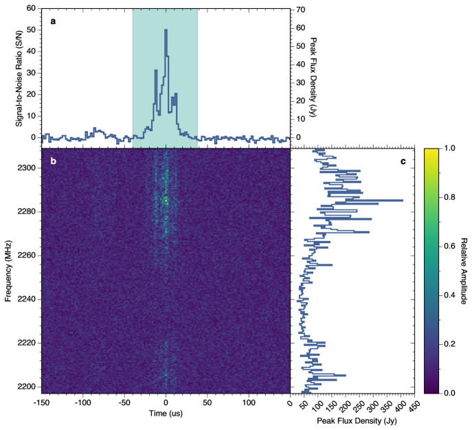
In Figure 1, we show the flux-calibrated dedispersed -band dynamic spectrum of the burst B1 using a DM value of 87.77 pc cm. In this case, we coherently dedispersed the baseband data to form filterbanks comprised of channelized power spectral densities with temporal and spectral resolutions of 2 s and 0.5 MHz, respectively. The frequency-averaged burst profile is shown in the upper panel, while the time-averaged on-pulse spectrum is shown in the right panel.
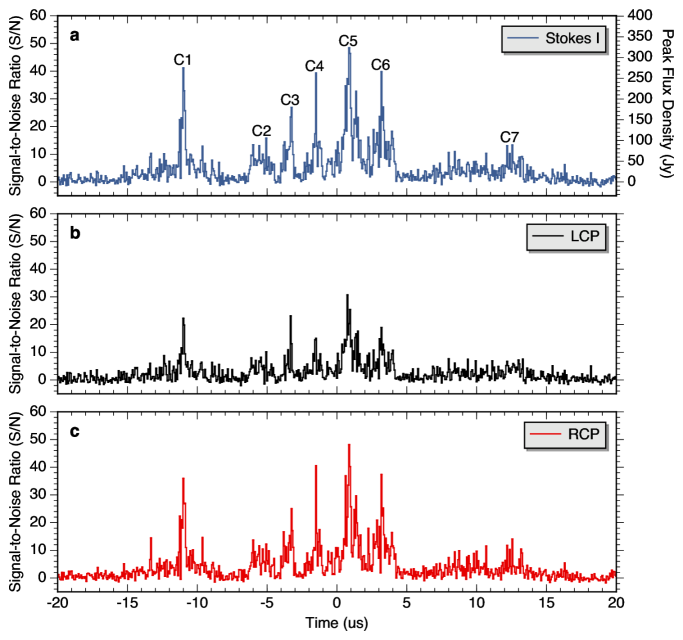
In Figure 2, we show the coherently dedispersed (87.77 pc cm) burst time series with 62.5 ns time resolution. The top panel shows the burst in flux-calibrated total intensity, while the lower panels show the right and left circular polarizations given in units of S/N. A detailed polarization analysis of B1 and additional bursts from this observation will be presented in a forthcoming publication.
The burst is made up of several remarkably narrow, isolated components, numbering at least seven non-overlapping components, labeled as C1-C7 in Figure 2. Component C1 is relatively narrow and appears to be preceded by a short period of low-level emission. This component is followed by a series of similarly narrow components with typical separation of 2-3 s. Component C4 is not resolved temporally with a width that is at least as short as the sampling time of 62.5 ns. The last component, C7, seems to be broader with a width of a few s. We also note the presence of a broad precursor emission in Figure 1, arriving s prior to the arrival time of B1. In Table 1, we list the peak time, peak S/N, DM value that maximized the peak S/N, burst width, burst peak flux density, and fluence. We also show in this table the flux density and fluence of the narrowest component of the burst, C4.
Although B1 was detected with high S/N at -band, there was no detectable signal during the same time at -band. Since no bursts were detected at -band, we place a 7- upper limit of 1.1 Jy on the flux density of the emission at 8.36 GHz during this observation, assuming a similar burst width of 33 s. At the narrowest component width (62.5 ns), corresponding to a single time sample in this observation, the 7- upper limit on the flux density at -band is 25 Jy.
If we further assume that the flux density of FRBs scales as a power-law (i.e., , where denotes the flux density at an observing frequency and is the spectral index), which is typical of most pulsar radio spectra, then we can place an upper limit of –1.3 on the spectral index of the emission process for the wider burst. On the other hand, using the measured flux density of the narrowest component at -band and assuming its width at -band is similarly narrow, we can place an upper limit of –1.8 on the spectral index of the emission process. However, we note that previous multi-wavelength observations of FRBs show patchy emission over large, instantaneous frequency bandwidths (Majid et al., 2020; Pearlman et al., 2020) and do not appear to support a power-law model (e.g., Spitler et al. 2016; Scholz et al. 2016; Law et al. 2017).
The burst spectrum (Figure 1) shows frequency structure on the order of 10 MHz across the band. Fitting Gaussians to the two bumps in the spectrum, we find full-width half-max values of MHz at MHz and MHz at MHz. This structure could be intrinsic or a result of diffractive interstellar scintillation. The NE2001 electron density model of the Milky Way (Cordes & Lazio, 2002) predicts that our Galaxy will impart a pulse broadening time of ns for an extragalactic source along the line of sight to this FRB (, ). Scaling to 2.3 GHz as , this gives ns, well below the time resolution of our data. The scintillation bandwidth corresponding to this scattering time is
| (1) |
which gives MHz at 2.3 GHz. The frequency structure we see in our burst spectrum is entirely consistent with modulation from scintillation, but measurements at other frequencies will be needed to confirm this. We note that the spectrum of B1 is not well modeled by a power law (i.e., , where denotes the flux density at an observing frequency and is the spectral index). This is also confirmed in previous studies of FRB spectra, where generally the burst spectra are not well modeled by a power law dependence (e.g., Scholz et al. 2016; Law et al. 2017; Majid et al. 2020). If the structure is indeed caused by scintillation, then this could also explain the lack of a detection at 8.36 GHz where the scintillation bandwidth would be GHz and we could have modulations in our band. However, FRBs are typically not broadband, so the lack of a detection at -band could also be explained by the intrinsic structure of the burst. Observations at other frequencies, particularly instantaneous broadband observations, will confirm whether the frequency structure we see in B1 at S-band along with a simultaneous lack of emission at X-band is indeed the result of scintillation or intrinsic structure of the burst. Similar narrow-band emission behavior has also been in seen in FRB 121102 and FRB 180916.J0158+65 , where detection of bright emission at lower frequencies have not been accompanied with emission at higher frequencies during simultaneous observations (Majid et al. 2020; Scholz et al. 2020; Pearlman et al. 2020).
| Peak Time (MJD) | 59275.99804894308a,g |
|---|---|
| DM | 87.77 0.02b |
| Peak S/N | 50.1c,g |
| Burst Width | 33 1 sd,g |
| Burst Peak Flux Density | 59 12 Jye,g |
| Burst Fluence | 0.76 0.15 Jy mse,f,g |
| Flux Density of Narrowest Component (C4) | 270 54 Jye,h |
| Fluence of Narrowest Component (C4) | 0.017 0.003 Jy mse,f,h |
Note. —
a Barycentric time of arrival (ToA) using the position RA (J2000) 09:57:56.7, Dec (J2000) 68:49:32.0 (Bhardwaj et al., 2021).
b DM value that maximized the peak S/N of the burst.
c Peak signal-to-noise ratio (S/N) after dedispersing with the peak S/N-maximizing DM of 87.77 pc cm.
d Burst width at 10 percent maximum.
e Uncertainties are dominated by the 20% fractional error on the system temperature, .
f Fluence determined using full width at 10% of peak SNR. This choice ensures that all of the burst energy is included.
g Value is derived from data sampled at a time resolution of 2 s.
h Value is derived from data sampled at a time resolution of 62.5 ns.
4. Discussion
High time resolution studies of FRBs are an important observational tool for discerning proposed emission mechanisms for FRBs, improving our ability to measure fundamental properties of FRBs such as burst energetics, shortest timescales of the emission process that could constrain the spatial sizes of the emission region, and burst energy densities. Furthermore, such high time resolution studies make it possible to carry out detailed studies of scatter broadening due to the turbulent plasma between the source and the observer, including studies of ISM in the Milky Way, the Milky Way halo, host galaxy halo, ISM in the host galaxy, and finally any local scattering material near the progenitors of FRBs. Finally, high time resolution studies of FRBs will also help in identifying known analogs to FRB emission characteristics, such as the giant-pulse phenomenon seen in some pulsars, Type III solar radio bursts, and short S-shaped decametric Jovian bursts (see, e.g., Hankins et al., 2015; Tan et al., 2019; Shaposhnikov et al., 2011).
4.1. Burst Microstructure
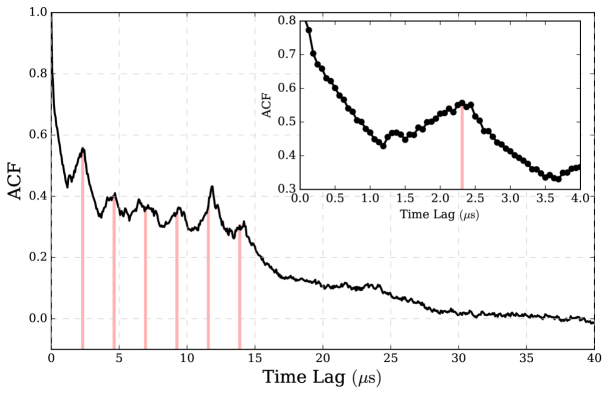
As shown in Figure 2, B1 is comprised of several narrow () components contained within a larger burst envelope (). In Figure 3, we show the autocorrelation function (ACF) of the total intensity burst B1. The ACF shows correlations out to time lags of and six peaks at time lags s. The peaks in the ACF have widths of 1–2 s and are roughly evenly spaced with separations of s. This is consistent with what we see in B1, where the seven components shown in Figure 2 have separations of 1.9–2.7 s (or integer multiples thereof). While the component separations are not strictly periodic in B1, there is clearly a repetition timescale of s in the burst structure.
The structure seen in B1 is qualitatively similar to what was seen in the scattering-limited observations of FRB 20180916B (Nimmo et al., 2021b), but on much longer time scales, and is strikingly similar to what is seen in some giant pulses from the Crab pulsar (Hankins et al., 2003; Hankins & Eilek, 2007). While the exact emission mechanism may not be the same between FRBs and Crab giant pulses, bursts from both sources are generically expected to be comprised of many individual shots of emission (Cordes & Wasserman, 2016). The small scattering towards FRB 20200120E and the high time resolution of these observations have enabled the clear detection of burst microstructure.
The roughly periodic occurrence of burst components within B1 is also reminiscent of the microstructure seen in single pulses of some radio pulsars. Pulsar microstructure describes the rapid intensity fluctuations within individual single pulses. ACF analyses like the one performed here have revealed that the microstructure of some pulsars has recurring periodicities (e.g., Cordes et al., 1990; Lange et al., 1998). While not seen in every radio pulsar, microstructure periodicities have been measured in several slow spinning pulsars (Lange et al., 1998; Mitra et al., 2015), the young Vela pulsar (Kramer et al., 2002), and even millisecond pulsars (De et al., 2016). Interestingly, there is a correspondence between the microstructure periodicity () and the pulsar spin period () given by
| (2) |
While it is not known if the origin of pulsar microstructure is geometric (beam sweeping past) or temporal modulation, the phenomenological similarity between B1 and periodic microstructure in pulsars is tantalizing and may suggest a magnetospheric origin for FRB 20200120E. If the structure seen in B1 follows the relation for pulsar microstructure, it would imply a spin period of several milliseconds, which could be achieved by a fast-spinning young pulsar or a recycled millisecond pulsar. The latter would be consistent with the localization of this FRB to a globular cluster (Kirsten et al., 2021b), which tend to be fertile grounds for the formation of millisecond pulsars.
4.2. Luminosity and Brightness Temperature
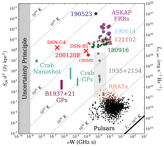
Figure 4 shows how the full burst B1 and its narrowest component C4 compared to other short duration radio pulses in the time-luminosity phase space. If we assume that the burst source is at the same distance as M81 ( Mpc), then B1 is on the faint end of the FRB luminosity distribution with a pseudo-luminosity of and an isotropic equivalent spectral luminosity of , which is only a factor of larger than the SGR 1935+2154 burst detected by STARE2 (Bochenek et al., 2020). Continued monitoring of this FRB with large telescopes will characterize the faint end of the FRB luminosity distribution to levels below the STARE2 burst.
The narrowest component, C4, has a pseudo-luminosity of and an isotropic equivalent spectral luminosity of . This is only times larger than the Crab nanoshot ( MJy, ns, kpc) seen by Hankins & Eilek (2007) and occupies the sparsely populated short duration region of the time-luminosity phase space (Figure 4). The brightness temperature, given by
| (3) |
is K for component C4, which is one of the highest measured values for any FRB and only a factor of smaller than the Crab nanoshot (Hankins & Eilek, 2007). Of course, since this narrow component is still unresolved in time, the true brightness temperature may be much larger.
4.3. Size of the Emission Region
Farah et al. (2018) reported the discovery of FRB 170827, which shows complex temporal structure with components as short as 30 s, indicating that the emission region may be as small as only 10 km. Similarly, Cho et al. (2020) showed the presence of microstructure in their study of FRB 181112, resolving emission components as short at 15 s, implying emission size of a few km. Nimmo et al. (2021b) reported on high time resolution observations of FRB 20180916B, where they observed several bursts with a range of timescales from a few ms to as short as a few s wide. Their observations, carried out at 1.7 GHz, were limited in resolving narrower structures by multi-path scattering. They attribute the observation of 3–4 s structure in one of the detected bursts to an emission region on the order of 1 km.
We are reporting a significantly shorter variability time scale for FRB 20200120E than for any previously published FRB. Very recently Nimmo et al. (2021a) also reported similar timescale emission for FRB 20200120E. While the envelope of emission spans , the burst is clearly comprised of distinct and non-overlapping narrow components. Using a light travel time argument, the short duration of the individual components imply small source sizes , where is the width of individual components. For an emission timescale of 100 ns, corresponding to the width of the narrowest component, the size of the emission region is constrained to be .
However, relativistic effects can significantly alter the relation between size of the emission region and the variability time scale. For instance, Beniamini & Kumar (2020) consider the case of a relativistic outflow moving with a Lorentz factor producing a radio burst at distance from the origin of the outflow, and define a characteristic time scale, ,
| (4) |
where the scaling has been chosen to give a timescale comparable to the shortest time scale observed in the burst reported here. Large or relatively small are required to explain variability time scales with . As discussed by Beniamini & Kumar (2020), the variability time scale may be even shorter than the characteristic time scale given in Eq, 4 due to a number of possible factors: clumps in the emission region, a narrow range of emission radii, radial evolution of the spectrum, or anisotropic emission. Given our observation that the burst components appear to have comparable rise and fall times, clumpiness or anisotropic emission would be favored over narrow emission radii or radial spectral evolution. In any case, as Beniamini & Kumar (2020) point out, the efficiency of conversion of energy from the relativistic outflow must decrease when a physical mechanism is invoked to decrease the time scale of variability.
4.4. Energy Density
Using the light travel time estimate, and combining the size of the emission region with the measured fluence (Table 1), we estimate the energy spectral density of the component to be in the rest frame of the emitting source. Under the conservative assumption that the emission is confined only to our observing band, we estimate the total energy density of the component to be . If we attribute the entire energy density to the equivalent energy density in a magnetic field , where B is the magnetic field and is the magnetic permeability, we obtain a magnetic field . We note that if relativistic effects such as beaming are taken into account (see the discussion in 4.3 above) the estimated magnetic field required to serve as the emission reservoir can be significantly lower than the value estimated above.
4.5. Propagation Effects
The extremely high time resolution of our data allows us to set a pulse broadening limit of ns to the total 2.3 GHz scattering along the line of sight to FRB 20200120E. Scaling to 1 GHz as , this corresponds to a limit of . A small scattering time is to be expected since the line of sight (, ) only passes through a small part of the Milky Way and the FRB likely resides in the outer edges of M81.
The NE2001 electron density model (Cordes & Lazio, 2002) predicts a Milky Way contribution to the 2.3 GHz pulse broadening time of ns at 2.3 GHz along the line of sight to the FRB. Although this is well below our time resolution limit, the corresponding scintillation bandwidth is MHz, which is entirely consistent with the frequency structure we see in B1. If there is any additional scattering caused by the host galaxy or the Milky Way halo (which is not modelled in NE2001), it would be limited to ns, which would correspond to a scintillation bandwidth of MHz at 2.3 GHz. We see no obvious signs of correlations on frequency separations less than MHz, which suggests that any additional scattering is smaller than the contribution from the Milky Way disk. This is consistent with the apparent location of the FRB outside M81 (Bhardwaj et al., 2021) and the small amount of scattering expected from the Milky Way halo (Ocker et al., 2021).
Observations at other frequencies will confirm whether the frequency structure we see in B1 is indeed the result of scintillation. Since the line of sight appears to be relatively uncontaminated by both the host and our own Galaxy, this FRB could be a very nice source for probing the properties of the ionized gas in the Galactic halo. Furthermore, the very small scattering seen here ( ns) means that even at 100 MHz the scattering would be ms. We therefore strongly encourage low frequency observations of FRB 20200120E for probing the Galactic halo.
4.6. Future Outlook
With the detection of unresolved burst structure at the native time resolution (62.5 ns) during the observations reported here, the question remains whether the individual components in bursts from FRB 20200120E are even narrower in width at nanosecond timescales. Such studies are best carried out at higher radio frequencies, where the effects of multi-path scatter broadening are mitigated. Since the temporal width of the bursts is a fundamental observational property of the emission processes and has important implications for determining the burst energetics, we encourage future observations of FRBs with even higher temporal resolutions at higher radio frequencies. On the other hand, as mentioned in the previous section, FRB 20200120E also offers an opportunity to study the properties of the ionized medium in the halo of the Milky Way Galaxy. Low frequency observations, where the effects of multi-path scattering are amplified, would also be quite useful for this purpose.
Acknowledgments
We thank Paz Beniamini and Sterl Phinney for informative discussions during the preparation of this paper.
A.B.P is a McGill Space Institute (MSI) Fellow and a Fonds de Recherche du Quebec – Nature et Technologies (FRQNT) postdoctoral fellow. R.S.W. is supported by an appointment to the NASA Postdoctoral Program at the Jet Propulsion Laboratory, administered by Universities Space Research Association under contract with NASA. M.B. is supported by an FRQNT Doctoral Research Award. C.L. was supported by the U.S. Department of Defense (DoD) through the National Defense Science and Engineering Graduate Fellowship (NDSEG) Program. E.P. acknowledges funding from an NWO Veni Fellowship.
We thank the Jet Propulsion Laboratory’s and California Institute of Technology’s President’s and Director’s Research and Development Fund for supporting this work. We also thank Dr. Charles Lawrence and Dr. Stephen Lichten for providing programmatic support. In addition, we are grateful to the DSN scheduling team (Hernan Diaz, George Martinez, Carleen Ward), the Madrid Deep Space Communication Complex (MDSCC) staff for scheduling and carrying out these observations, and Steven Olson for his help in flux calibration of the data.
A portion of this research was performed at the Jet Propulsion Laboratory, California Institute of Technology and the Caltech campus, under a Research and Technology Development Grant through a contract with the National Aeronautics and Space Administration. U.S. government sponsorship is acknowledged.
FRB research at UBC is supported by an NSERC Discovery Grant and by the Canadian Institute for Advanced Research.
References
- Bannister et al. (2019) Bannister, K. W., Deller, A. T., Phillips, C., et al. 2019, Science, 365, 565
- Beniamini & Kumar (2020) Beniamini, P., & Kumar, P. 2020, MNRAS, 498, 651
- Bhardwaj et al. (2021) Bhardwaj, M., Gaensler, B. M., Kaspi, V. M., et al. 2021, ApJ, 910, L18
- Bochenek et al. (2020) Bochenek, C. D., Ravi, V., Belov, K. V., et al. 2020, Nature, 587, 59
- Chatterjee et al. (2017) Chatterjee, S., Law, C. J., Wharton, R. S., et al. 2017, Nature, 541, 58
- CHIME/FRB Collaboration et al. (2020) CHIME/FRB Collaboration, Andersen, B. C., Bandura, K. M., et al. 2020, Nature, 587, 54
- Cho et al. (2020) Cho, H., Macquart, J.-P., Shannon, R. M., et al. 2020, ApJ, 891, L38
- Cordes & Chatterjee (2019) Cordes, J. M., & Chatterjee, S. 2019, ARA&A, 57, 417
- Cordes & Lazio (2002) Cordes, J. M., & Lazio, T. J. W. 2002, arXiv e-prints, arXiv:astro–ph/0207156
- Cordes & Wasserman (2016) Cordes, J. M., & Wasserman, I. 2016, MNRAS, 457, 232
- Cordes et al. (1990) Cordes, J. M., Weisberg, J. M., & Hankins, T. H. 1990, AJ, 100, 1882
- De et al. (2016) De, K., Gupta, Y., & Sharma, P. 2016, ApJ, 833, L10
- Farah et al. (2018) Farah, W., Flynn, C., Bailes, M., et al. 2018, MNRAS, 478, 1209
- Fonseca et al. (2020) Fonseca, E., Andersen, B. C., Bhardwaj, M., et al. 2020, ApJ, 891, L6
- Gajjar et al. (2018) Gajjar, V., Siemion, A. P. V., Price, D. C., et al. 2018, ApJ, 863, 2
- Hankins & Eilek (2007) Hankins, T. H., & Eilek, J. A. 2007, ApJ, 670, 693
- Hankins et al. (2015) Hankins, T. H., Jones, G., & Eilek, J. A. 2015, ApJ, 802, 130
- Hankins et al. (2003) Hankins, T. H., Kern, J. S., Weatherall, J. C., & Eilek, J. A. 2003, Nature, 422, 141
- Karuppusamy et al. (2010) Karuppusamy, R., Stappers, B. W., & van Straten, W. 2010, A&A, 515, A36
- Kirsten et al. (2021a) Kirsten, F., Snelders, M. P., Jenkins, M., et al. 2021a, Nature Astronomy, 5, 414
- Kirsten et al. (2021b) Kirsten, F., Marcote, B., Nimmo, K., et al. 2021b, arXiv e-prints, arXiv:2105.11445
- Kramer et al. (2002) Kramer, M., Johnston, S., & van Straten, W. 2002, MNRAS, 334, 523
- Lange et al. (1998) Lange, C., Kramer, M., Wielebinski, R., & Jessner, A. 1998, A&A, 332, 111
- Law et al. (2017) Law, C. J., Abruzzo, M. W., Bassa, C. G., et al. 2017, ApJ, 850, 76
- Lundgren et al. (1995) Lundgren, S. C., Cordes, J. M., Ulmer, M., et al. 1995, ApJ, 453, 433
- Majid et al. (2011) Majid, W. A., Naudet, C. J., Lowe, S. T., & Kuiper, T. B. H. 2011, ApJ, 741, 53
- Majid et al. (2020) Majid, W. A., Pearlman, A. B., Nimmo, K., et al. 2020, ApJ, 897, L4
- Manchester et al. (2005) Manchester, R. N., Hobbs, G. B., Teoh, A., & Hobbs, M. 2005, AJ, 129, 1993
- Marcote et al. (2020) Marcote, B., Nimmo, K., Hessels, J. W. T., et al. 2020, Nature, 577, 190
- Marthi et al. (2020) Marthi, V. R., Gautam, T., Li, D. Z., et al. 2020, MNRAS, 499, L16
- McKee et al. (2019) McKee, J. W., Stappers, B. W., Bassa, C. G., et al. 2019, MNRAS, 483, 4784
- Mitra et al. (2015) Mitra, D., Arjunwadkar, M., & Rankin, J. M. 2015, ApJ, 806, 236
- Nimmo et al. (2021a) Nimmo, K., Hessels, J. W. T., Kirsten, F., et al. 2021a, arXiv e-prints, arXiv:2105.11446
- Nimmo et al. (2021b) Nimmo, K., Hessels, J. W. T., Keimpema, A., et al. 2021b, Nature Astronomy, arXiv:2010.05800 [astro-ph.HE]
- Ocker et al. (2021) Ocker, S. K., Cordes, J. M., & Chatterjee, S. 2021, ApJ, 911, 102
- Pearlman et al. (2020) Pearlman, A. B., Majid, W. A., Prince, T. A., et al. 2020, ApJ, 905, L27
- Petroff et al. (2019) Petroff, E., Hessels, J. W. T., & Lorimer, D. R. 2019, A&A Rev., 27, 4
- Petroff et al. (2016) Petroff, E., Barr, E. D., Jameson, A., et al. 2016, PASA, 33, e045
- Platts et al. (2019) Platts, E., Weltman, A., Walters, A., et al. 2019, Phys. Rep., 821, 1
- Prochaska et al. (2019) Prochaska, J. X., Macquart, J.-P., McQuinn, M., et al. 2019, Science, 366, 231
- Ravi et al. (2019) Ravi, V., Catha, M., D’Addario, L., et al. 2019, Nature, 572, 352
- Scholz et al. (2016) Scholz, P., Spitler, L. G., Hessels, J. W. T., et al. 2016, ApJ, 833, 177
- Scholz et al. (2017) Scholz, P., Bogdanov, S., Hessels, J. W. T., et al. 2017, ApJ, 846, 80
- Scholz et al. (2020) Scholz, P., Cook, A., Cruces, M., et al. 2020, ApJ, 901, 165
- Shaposhnikov et al. (2011) Shaposhnikov, V. E., Korobkov, S. V., Rucker, H. O., et al. 2011, Journal of Geophysical Research (Space Physics), 116, A03205
- Spitler et al. (2016) Spitler, L. G., Scholz, P., Hessels, J. W. T., et al. 2016, Nature, 531, 202
- Tan et al. (2019) Tan, B., Chen, N., Yang, Y.-H., et al. 2019, ApJ, 885, 90
- The CHIME/FRB Collaboration et al. (2019a) The CHIME/FRB Collaboration, Amiri, M., Bandura, K., et al. 2019a, Nature, 566, 235
- The CHIME/FRB Collaboration et al. (2019b) The CHIME/FRB Collaboration, Andersen, B. C., Bandura, K., et al. 2019b, ApJ, 885, L24
- Zhang et al. (2020) Zhang, C. F., Jiang, J. C., Men, Y. P., et al. 2020, The Astronomer’s Telegram, 13699, 1