A test of the evolution of gas depletion factor in galaxy clusters using strong gravitational lensing systems

Abstract

In this blackwork, we discuss a new method to probe the redshift evolution of the gas depletion factor, i.e. the ratio by which the gas mass fraction of galaxy clusters is depleted with respect to the universal mean of baryon fraction. The dataset we use for this purpose consists of 40 gas mass fraction measurements measured at $r_{2500}$ using Chandra X-ray observations, strong gravitational lensing sub-samples obtained from SLOAN Lens ACS + BOSS Emission-line Lens Survey (BELLS) + Strong Legacy Survey SL2S + SLACS. For our analysis, the validity of the cosmic distance duality relation is assumed. We find a mildly decreasing trend for the gas depletion factor as a function of redshift at about 2.7$\sigma$.

I Introduction

Galaxy clusters are the largest gravitationally bound structures in the Universe, and hence are a powerful probe of the evolution and structure formation in the Universe at redshifts $z<2$ (see Mantz et al. (2014); Vikhlinin et al. (2014) for detailed reviews). They are also wonderful laboratories for fundamental Physics measurements Carbone et al. (2012); Desai (2018) One can obtain constraints on the cosmological parameters, if we assume that the X-ray gas mass fraction, $f_{gas}$, of hot, massive and relaxed galaxy clusters does not evolve with redshift Sasaki (1996); Allen et al. (2007); Ettori et al. (2009); Mantz et al. (2014); Pen (1997); White et al. (1993). In order to quantify the baryon content and its possible time evolution, crucial to cosmological tests with gas mass fraction measurements, hydrodynamic simulations have been used to calibrate the gas depletion factor, $g(z)$, viz. the ratio by which the gas mass fraction of galaxy clusters is depleted with respect to the universal mean of the baryon fraction. Planelles et al. (2013) and Battaglia et al. (2013), have previously shown using simulations of hot, massive, and dynamically relaxed galaxy clusters ($M_{500}>10^{14}M_{\odot}$) involving different physical processes, that by modelling a possible time evolution for $g(z)$, given by $g(z)\equiv g_{0}(1+g_{1}z)$ , one obtains: $0.55\leq g_{0}\leq 0.79$ and $-0.04\leq g_{1}\leq 0.07$, depending on the physical processes that are included in the simulations (see Table 3 in (Planelles et al., 2013) for values obtained at $r_{2500}$). Therefore, no significant trend of $g(z)$ as a function of redshift was found in their simulations. For their analysis,  Planelles et al. (2013) considered $f_{gas}$ as a cumulative quantity up to $r_{2500}$, the radii at which the mean cluster density is 2500 times the critical density of the Universe at the cluster’s redshift. Recently, by using the cosmo-OverWhelmingly Large Simulation, the Ref. Le Brun et al. (2017) showed that in most realistic models of intra-cluster medium, which include active galactic nuclei feedback, the slopes of the various mass-observable relations deviate substantially from the self-similar one. Self-similarity implies that galaxy clusters are identical objects when scaled by their mass Kaiser (1986), or in other words, galaxy clusters form via a single gravitational collapse, particularly at late times and for low-mass clusters. A constant non-varying gas depletion factor is also expected from self-similarity Mohr et al. (1999).

On the other hand, there have been a number of works, which have estimated the depletion factor directly from observations, without using simulations. For instance, the Ref.Holanda et al. (2017) carried out an analysis using 40 $f_{gas}$ measurements observed by the Chandra X-ray telescope provided by the Ref. Mantz et al. (2014) along with Type Ia supernovae observations, with priors on $\Omega_{b}$ and $\Omega_{M}$ from the Planck results Planck Collaboration et al. (2016), and assuming the validity of the cosmic distance duality relation (CDDR) Ellis (2007). No evolution of the gas depletion factor with redshift was found from this aforementioned analysis. In a follow-up work, Ref. Holanda (2018) used a completely independent set of 38 Chandra X-ray $f_{gas}$ measurements in the redshift range $0.14\leqslant z\leqslant 0.89$ provided by the Ref. LaRoque et al. (2006), along with angular diameter distances from X-ray/SZ measurements and priors from Planck results Planck Collaboration et al. (2016). Unlike Holanda et al. (2017), they did not use CDDR to derive the angular diameter distance. The aforementioned work reported $g_{0}$ = $0.76\pm 0.14$ and $g_{1}$ = $-0.42_{-0.40}^{+0.42}$, which also implies no redshift evolution for the gas depletion factor. The gas mass fractions calculated by the Ref. LaRoque et al. (2006) were obtained within $r_{2500}$, while those from the Ref. Mantz et al. (2014) were calculated in spherical shells at radii near $r_{2500}$.

Constraints on the evolution of $g(z)$ using gas mass fraction measurements within $r_{500}$ have also been obtained. Zheng et al. (2019) used 182 galaxy clusters detected by the Atacama Cosmology Telescope Polarization experiment Hilton et al. (2018) and cosmic chronometers Jimenez and Loeb (2002), and found a mild decrease of $g(z)$ as a function of redshift ( $g(z)$ is smaller at high z). Most recently, Bora and Desai (2021a) also looked for a time evolution of $g(z)$ using gas mass fraction measurements at $r_{500}$, from both the SPT-SZ Chiu et al. (2018) and Planck Early Sunyaev-Zeldovich effect cluster data Planck Collaboration et al. (2011) along with cosmic chronometers and priors from Planck results Planck Collaboration et al. (2020). Conflicting results between both the samples were found: for SPT-SZ, $g(z)$ was found to be decreasing as a function of redshift (at more than 5$\sigma$), whereas a positive trend with redshift was found for Planck ESZ data (at more than 4$\sigma$). Their results implied that one cannot use $f_{gas}$ values at $r_{500}$ as a stand-alone probe for any model-independent cosmological tests.

In this letter, we propose a new observational test for the time evolution of the gas depletion factor by using multiple large scale structure probes, namely, galaxy cluster gas mass fraction measurements Mantz et al. (2014) along with strong gravitational lenses (SGL) observations obtained from SLOAN Lens ACS + BOSS Emission-line Lens Survey (BELLS) + Strong Legacy Survey SL2S + SLACS Leaf and Melia (2018). For our analysis, we assume the validity of the CDDR Ellis (2007). By considering a possible time evolution for $g(z)$, such as $g(z)=g_{0}(1+g_{1}z)$, and analyses by using three SGL sub-samples separately (segregated according to their mass intervals), we obtain an error-weighted average given by: $g_{1}=-0.15\pm 0.055$ at $1\sigma$ c.l. Therefore, we infer a mild time evolution at about $2.7\sigma$ from our analysis. We note that unlike previous works in this area, our results are independent of the Planck cosmological parameters ($\Omega_{b}$ and $\Omega_{M}$). However, a flat universe model with $\Omega_{tot}=1$ is still assumed.

This letter is organized as follows. Section II explains the methodology adopted in this work. In section III, we present the data sample used for our analysis. Section IV describes our analysis and results. Our conclusions are presented in Section V.

II Methodology

In this section, we discuss some aspects of SGL systems and gas mass fractions, and show how one can combine these observations in order to put constraints on the gas depletion factor.

II.1 Strong Gravitational Lensing Systems

Strong gravitational lensing has proved to be a powerful diagnostic of modified gravity theories and cosmological models, as well as fundamental physics Schneider et al. (1992); Bartelmann (2010). blackThese systems have been used to constrain the PPN $\gamma$ parameter, cosmic curvature Kumar et al. (2021); Wei et al. (2022); Wang et al. (2020a); Cao et al. (2017), variations of speed of light Liu et al. (2021a), variations of fine structure constant Colaço et al. (2021), Hubble constant Qi et al. (2021), tests of FLRW metric Cao et al. (2019), etc. Usually, a strong lens system consists of a foreground galaxy or a cluster of galaxies positioned between a source (quasar) and an observer, where the multiple-image separation from the source depends only on the lens and the source angular diameter distance (see, for instance, Refs. Futamase and Yoshida (2001); Biesiada (2006); Grillo et al. (2008); Cao et al. (2012, 2015); Holanda et al. (2017a); Cao et al. (2018); Amante et al. (2020); Lizardo et al. (2021); Bora et al. (2021), where SGL systems were used recently as a cosmological tool). By using the simplest model assumption (the singular isothermal sphere) to describe the SGL systems, the Einstein radius ($\theta_{E}$), a fundamental quantity, can be defined as Bartelmann (2010); Cao et al. (2015):

$$\theta_{E}=4\pi\frac{D_{A_{ls}}}{D_{A_{s}}}\frac{\sigma_{SIS}^{2}}{c^{2}}$$ (1)

In this equation, $D_{A_{ls}}$ is the angular diameter distance from the lens to the source; $D_{A_{s}}$ denotes the angular diameter distance from the observer to the source; $\sigma_{SIS}$ is the velocity dispersion caused by the lens mass distribution; and $c$ is the speed of light.

For our analyses, a flat universe is considered and the following observational quantity derived for SGL systems is used Liao (2019):

$$D={\frac{D_{A_{ls}}}{D_{A_{s}}}}=\frac{{\theta}_{E}c^{2}}{4{\pi}\sigma^{2}_{SIS}}$$ (2)

For a flat universe, the comoving distance $r_{ls}$ is given by $r_{ls}=r_{s}-r_{l}$ Bartelmann (2010), and using $r_{s}=(1+z_{s})D_{A_{s}}$, $r_{l}=(1+z_{l})D_{A_{l}}$ and $r_{ls}=(1+z_{s})D_{A_{ls}}$, we obtain the following:

$$D=1-\frac{(1+z_{l})D_{A_{l}}}{(1+z_{s})D_{A_{s}}}$$ (3)

Finally, by the validity of the CDDR relation $D_{L}=(1+z)^{2}D_{A}$ Ellis (2007), Eq. 3 can be re-cast as follows:

$$\frac{(1+z_{s})}{(1+z_{l})}=(1-D)\frac{D_{L_{s}}}{D_{L_{l}}}$$ (4)

II.2 Gas mass fraction

The cosmic gas mass fraction can be defined as $f_{gas}\equiv\Omega_{b}/\Omega_{M}$ (where $\Omega_{b}$ and $\Omega_{M}$ are the baryonic and total matter density parameters, respectively), and the constancy of this quantity within massive, relaxed clusters within $r_{2500}$ has been used to constrain cosmological parameters by using the following equation (see, for instance, Mantz et al. (2014))

$$f_{gas}(z)=A(z)Kg(z)\left[\frac{\Omega_{b}}{\Omega_{M}}\right]\left(\frac{D_{L}^{*}}{D_{L}}\right)^{3/2}\$$ (5)

Here, the observations are done in the X-ray band. The asterisk in Eq. 5 denotes the corresponding quantities for the fiducial model used in the observations to obtain $f_{gas}$ (usually a flat $\Lambda$CDM model with Hubble constant $H_{0}=70$ km s^-1 Mpc^-1 and the present-day total matter density parameter $\Omega_{M}=0.3$), $A(z)$ represents the angular correction factor, which is very close to unity in almost all the cases, and hence can be neglected. The $K$ factor is the instrument calibration constant, which also accounts for any bias in the mass due to non-thermal pressure and bulk motions in the baryonic gas Allen et al. (2007); Mantz et al. (2014); Planelles et al. (2013); Battaglia et al. (2013). Twelve galaxy clusters used in this present work are also part of the “Weighing the Giants” sample Applegate et al. (2016), and this work found the $K$ factor to be constant, i.e., no significant trends with mass, redshift, or any morphological indicators were found. Therefore, we also posit the same in this work. The quantity $g(z)$, which is of interest here is again modelled in the same way as previous works, i.e. $g(z)=g_{0}(1+g_{1}z)$. The ratio in the parenthesis of Eq. 5 encapsulates the expected variation in $f_{gas}$ when the underlying cosmology is varied, which makes the analyses with gas mass fraction measurements model-independent. Finally, it is important to stress that Eq. 5 is obtained only after assuming the validity of CDDR (see Ref. Gonçalves et al. (2012) for details). In the last decade, a plethora of analyses using myriad observational data have been undertaken in order to establish whether or not the CDDR holds in practice. A succinct summary of the latest observational constraints on the CDDR can be found in Refs.Holanda et al. (2022); Bora and Desai (2021b), which demonstrate the validity of CDDR to within 2$\sigma$.

The key equation to our method can be obtained from combining Eq. 4 and 5, and by incorporating a possible redshift dependence for the gas depletion factor, such as $g(z)=g_{0}(1+g_{1}z)$. In this way, we now obtain:

$$\left[\frac{(1+g_{1}z_{s})}{(1+g_{1}z_{l})}\right]=\left[\frac{f_{gas}(z_{s})}{f_{gas}(z_{l})}\right]\left[\frac{(1+z_{s})D^{*}_{L_{l}}}{(1+z_{l})D^{*}_{L_{s}}}\right]^{3/2}(1-D)^{-3/2}$$ (6)

As we can see, unlike Ref.Holanda et al. (2017b); Bora and Desai (2021a), our results are independent of the $K$ factor, $g_{0}$, and $\Omega_{b}/\Omega_{M}$.

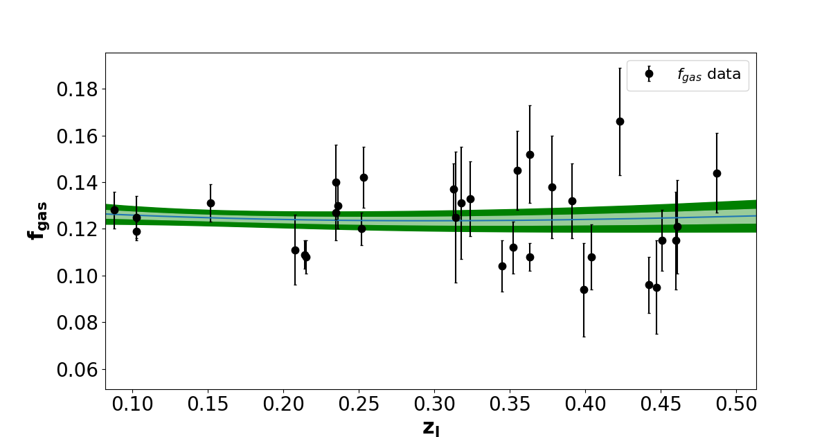
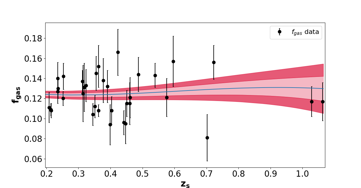
Figure 1: (Left) Reconstruction of the gas mass fraction at $z_{l}$ for the Intermediate Mass range sample using Gaussian Process Regression. The green shaded area indicates 1$\sigma$ and 2 $\sigma$ error bands. (Right) Reconstruction of the gas mass fraction at $z_{s}$ for the Intermediate Mass range sample using Gaussian Process Regression. The crimson shaded area indicates 1 $\sigma$ and 2 $\sigma$ error bands.

III Cosmological data

The data used in our analysis were as follows:

• 40 X-ray gas mass fraction measurements of hot ($kT\geq 5$ keV), massive and morphologically relaxed galaxy clusters from archival Chandra data.  blackThe exposure times range from 7-350 ksec. (cf Table 1 of  Mantz et al. (2014)). The morphological diagnostics used to identify relaxed clusters are discussed in  Mantz et al. (2015). The galaxy cluster redshift range is $0.078\leq z\leq 1.063$ Mantz et al. (2014) black The restriction to relaxed systems minimizes the systematic biases due to departures from hydrostatic equilibrium and substructure, as well as the scatter due to these effects, asphericity, and projection. The bias in the mass measurements from X-ray data arising by assuming hydrostatic equilibrium was calibrated using robust mass estimates for the target clusters from weak gravitational lensing Applegate et al. (2016), reducing systematic uncertainties. Furthermore, these authors measured the gas mass fraction in spherical shells at radii near at $r_{2500}$ ($\approx 1/4$ of virial radius), instead of using the cumulative fraction integrated over all radii ($<r_{2500}$) as in several previous works present in literature. The data were fitted with a non-parametric model for the deprojected, spherically symmetric intracluster medium density and temperature profiles. In this model, the cluster atmosphere is described as a set of concentric, spherical shells (near at $r_{2500}$), and, within each shell, the gas is assumed to be isothermal (see more details in Mantz et al. (2016)). Therefore the gas mass fraction is agnostic to details of the temperature and gas density profile of the sort discussed in  Cao et al. (2016a); Cao and Zhu (2011), which would mainly affect gas mass fraction measurements only at $R_{500}$. As pointed by these authors, the observations were restricted to the most self-similar and accurately measured regions of clusters, significantly reducing systematic uncertainties compared to previous work. The dark matter profile of the clusters were modeled by the so-known Navarro-Frank-White form.

• We also consider sub-samples from a specific catalog containing 158 confirmed sources of strong gravitational lensing systems Chen et al. (2019); Leaf and Melia (2018). This compilation includes 118 SGL systems identical to the compilation of Cao et al. (2015), which was obtained from a combination of SLOAN Lens ACS, BOSS Emission-line Lens Survey (BELLS), and Strong Legacy Survey SL2S, along with 40 additional systems recently discovered by SLACS and pre-selected by Shu et al. (2017) (see Table I in Leaf and Melia (2018)). Several studies have shown that the slopes of the density profiles for individual galaxies show a non-negligible deviation from the Singular isothermal sphere profile Koopmans et al. (2009); Auger et al. (2010); Barnabè et al. (2011); Sonnenfeld et al. (2013); Cao et al. (2016b); Holanda et al. (2017); Chen et al. (2019). Therefore, for the mass distribution of lensing systems, the power-law model is assumed. This model considers a spherically symmetric mass distribution with a more general power-law index $\gamma$, namely $\rho\propto r^{-\gamma}$. In this approach $\theta_{E}$ is given by:

  $$\theta_{E}=4\pi\frac{\sigma_{ap}^{2}}{c^{2}}\frac{D_{ls}}{D_{s}}\left[\frac{\theta_{E}}{\theta_{ap}}\right]^{2-\gamma}f(\gamma),$$ (7)

  where $\sigma_{ap}$ is the stellar velocity dispersion inside an aperture of size $\theta_{ap}$ and

  $$f(\gamma) = -\frac{1}{\sqrt{\pi}}\frac{(5-2\gamma)(1-\gamma)}{(3-\gamma)}\frac{\Gamma(\gamma-1)}{\Gamma(\gamma-3/2)}$$ (8)

  $$\times \left[\frac{\Gamma(\gamma/2-1/2)}{\Gamma(\gamma/2)}\right]^{2}$$

  Thus, we obtain:

  $$D=\frac{D_{A_{ls}}}{D_{A_{s}}}=\frac{c^{2}\theta_{E}}{4\pi\sigma_{ap}^{2}}\left[\frac{\theta_{ap}}{\theta_{E}}\right]^{2-\gamma}f^{-1}(\gamma)$$ (9)

  For $\gamma=2$, the singular isothermal spherical distribution is recovered. All the terms necessary to evaluate $D$ can be found in Table 1 of Leaf and Melia (2018). However, the complete dataset (158 points) is culled to 98 points, after the following cuts: $z<1.061$ and $D\pm\sigma_{D}<1$ ($D>1$ represents a non-physical region). The compilation considered here contains only those SGL systems with early type galaxies acting as lenses. Each data point contains estimated apparent and Einstein radius, with spectroscopically measured stellar apparent velocity dispersion, as well as both the lens and the source redshifts.

  We should point out that some works have recently explored a possible time evolution of the mass density power-law index Cao et al. (2016b); Holanda et al. (2017); Amante et al. (2020); Chen et al. (2019). No significant evolution has been found in these works. On the other hand, these results indicate that it is prudent to use low, intermediate, and high-mass galaxies separately in any cosmological analyses. As commented in Cao et al. (2016b), elliptical galaxies with velocity dispersions smaller than $200$ km/s may be classified roughly as relatively low-mass galaxies, while those with velocity dispersion larger than $300$ km/s may be treated as relatively high-mass galaxies. Naturally, elliptical galaxies with velocity dispersion between $200-300$ km/s may be classified as intermediate-mass galaxies. Therefore, in our analyses, we work with three distinct sub-samples consisting of 26, 63, and 9 data points with low, intermediate, and high velocity dispersions, respectively. The redshift range covered by these three samples is shown in Figure 2. As we can see, all the three samples cover roughly the same redshift range.

  To constrain $g_{1}$ by using Eq. 6, gas mass fraction measurements at the lens and source redshifts (for each SGL system) are required. These quantities are obtained by applying Gaussian Process Regression (GPR) Seikel et al. (2012); Singirikonda and Desai (2020) using the 40 gas mass fraction measurements compiled by Ref.Mantz et al. (2014) in order to estimate the gas mass fraction at any arbitrary redshift. In Fig. 1, we show the result of reconstruction of the gas mass fraction at $z_{l}$ and $z_{s}$ from the Intermediate Mass Range SGL sub-sample for the purpose of illustration. A discussion of GPR and comparison with other non-parametric regression techniques such as ANN can be found in the Appendix. The final results will also be sensitive to the choice of the reconstruction technique.

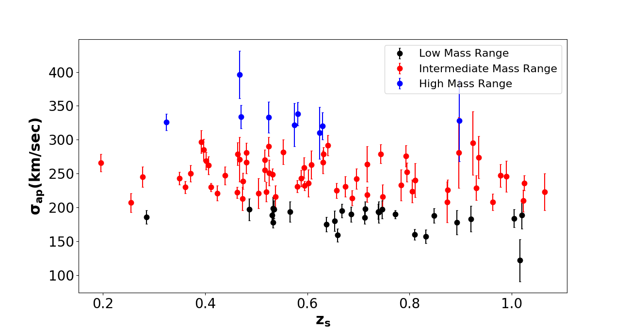
Figure 2: The different redshifts range covered by Low, Intermediate, and High mass range SGL sample.

Table 1: . Constraints on the parameters $\gamma$ and $g_{1}$ for different $\sigma_{ap}$ range used in this analysis as discussed in Sect. IV.

Sample	$\sigma_{ap}$(km/sec)	$\gamma$	$g_{1}$
Low	$\sigma_{ap}<200$	$1.913^{+0.009}_{-0.010}$	$0.172^{+0.173}_{-0.167}$
Intermediate	$200<\sigma_{ap}<300$	$2.041\pm 0.012$	$-0.188^{+0.060}_{-0.059}$
High	$\sigma_{ap}>300$	$1.983^{+0.082}_{-0.081}$	$-0.137^{+0.319}_{-0.254}$

IV Analysis and Results

The joint constraints on the power law index, $\gamma$ and redshift dependent part of the gas depletion factor, $g_{1}$ can be obtained by maximizing the likelihood distribution function, ${\cal{L}}$ given by

$$-2\ln\mathcal{L}=\sum_{i=1}^{n}\ln 2\pi{\sigma_{i}^{2}}+\sum_{i=1}^{n}\frac{\left(\Phi(g_{1},z_{i})-\left[\frac{f_{gas}(z_{s})}{f_{gas}(z_{l})}\right]\left[\frac{(1+z_{s})D^{*}_{L_{l}}}{(1+z_{l})D^{*}_{L_{s}}}\right]^{3/2}(1-D)^{-3/2}\right)^{2}}{\sigma_{i}^{2}},$$ (10)

where

$$\Phi(g_{1},z_{i})=\left[\frac{(1+g_{1}z_{s})}{(1+g_{1}z_{l})}\right]$$ (11)

Here, $\sigma_{i}$ denotes the statistical errors associated with the gravitational lensing observations (see Table A1 from Chen et al. (2019)) and gas mass fraction measurements (see table II in Mantz et al. (2014)), and are obtained by using standard propagation errors techniques. We have assumed that the errors in the gas mass fraction measurements and lensing observations are uncorrelated, as they correspond to to different systems. The distribution of errors in $f_{gas}$ at $z_{l}$ and $z_{s}$ can be found in the left panel of Figure 3, whereas the same for errors in the velocity dispersion, $\sigma_{ap}$ can be found in the right panel of Figure 3. We can see that the errors are roughly comparable for all the data points, so that no one system will dominate the results. Note that the quantity $D$ that appears in the log-likelihood (Eq. 10) depends on the parameter $\gamma$ via Eq. 9. The value of $n$ is equal to 26, 63, 9 for the low, intermediate, and high velocity dispersions, respectively. We maximize our likelihood function using the $\tt{emcee}$ MCMC sampler Foreman-Mackey et al. (2013) in order to estimate the free parameters used in Eq. 10, viz. $\gamma$ and $g_{1}$.

The one-dimensional marginalized posteriors for each parameter along with the 68%, 95%, and 99% 2-D marginalized credible intervals, are shown in Fig. 4, Fig. 5, and Fig. 6 for the Low, Intermediate, and High samples, respectively. As we can see, the analyses with the low and high mass SGL sub-samples are in full agreement with no evolution for the depletion factor, while the intermediate sub-sample shows a non-negligible evolution of $g(z)$ (see Table 1). We calculate an error-weighted average using the three estimates and obtained: $g_{1}=-0.15\pm 0.055$ at 1$\sigma$, showing a mild evolution for $g(z)$ at 2.7$\sigma$. (see Fig. 7).

We should point out that although a non-constant gas depletion factor has previously been obtained using measurements within $r_{500}$ Zheng et al. (2019); Bora and Desai (2021a), this is the first result which finds a time-varying depletion factor, using gas mass fraction measurements in spherical shells at radii near $r_{2500}$. Previous works Planelles et al. (2013); Battaglia et al. (2013) using cosmological hydrodynamic simulations did not find a significant trend of $g(z)$ as a function of redshift for gas mass fraction measurements within $r_{2500}$ or $r_{500}$ (see, for instance, the Tables II and III from the Ref. Planelles et al. (2013)). Therefore, our results are in tension with these results from cosmological simulations. However, it is important to comment that the models describing the physics of the intra-cluster medium used in hydrodynamic simulations may not span the entire range of physical process allowed by our current understanding.

Finally, as we can see, the high SGL sub-sample is in full agreement with the SIS model ($\gamma=2$) (cf. Table 1) while the low and intermediate mass SGL sub-samples are not compatible with this model even at 3$\sigma$ c.l.. Therefore, our results also reinforce the need for segregating the lenses into low, intermediate, and high velocity dispersions, and analyzing them separately. As we obtain a mild evolution for the gas depletion factor for Intermediate Mass Sample, as a sanity check, we also look for the redshift dependence of the parameter $\gamma$ for the Intermediate mass sample. For this purpose, we posit a parametric form: $\gamma(z)=\gamma_{0}+\gamma_{1}z_{l}$ and set $\gamma_{0}$ and $\gamma_{1}$ as the free parameters along with gas depletion factor $g_{1}$. We get: $\gamma_{0}=2.069\pm 0.027$, $\gamma_{1}=-0.159\pm 0.142$ and $g_{1}=-0.184\pm 0.06$ as shown in Figure 8. We found a marginal decrease for $\gamma$ with redshift at 1.1$\sigma$. As we can see, we still get a mild evolution of gas depletion factor at 3.1$\sigma$.

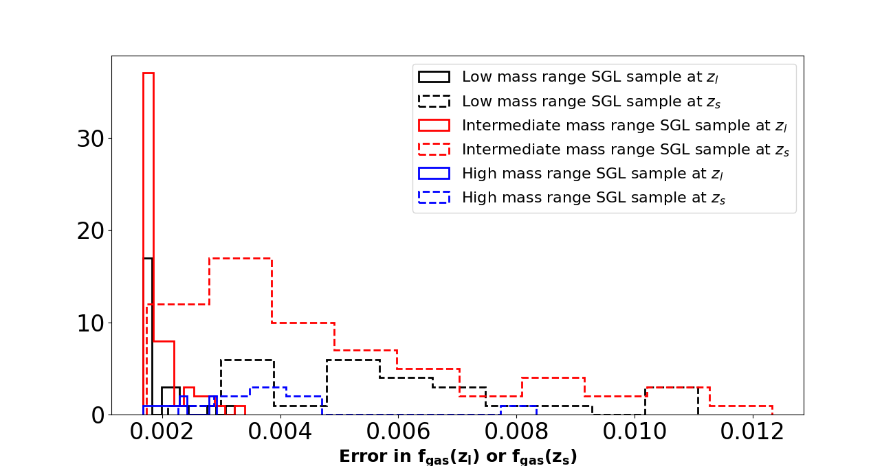
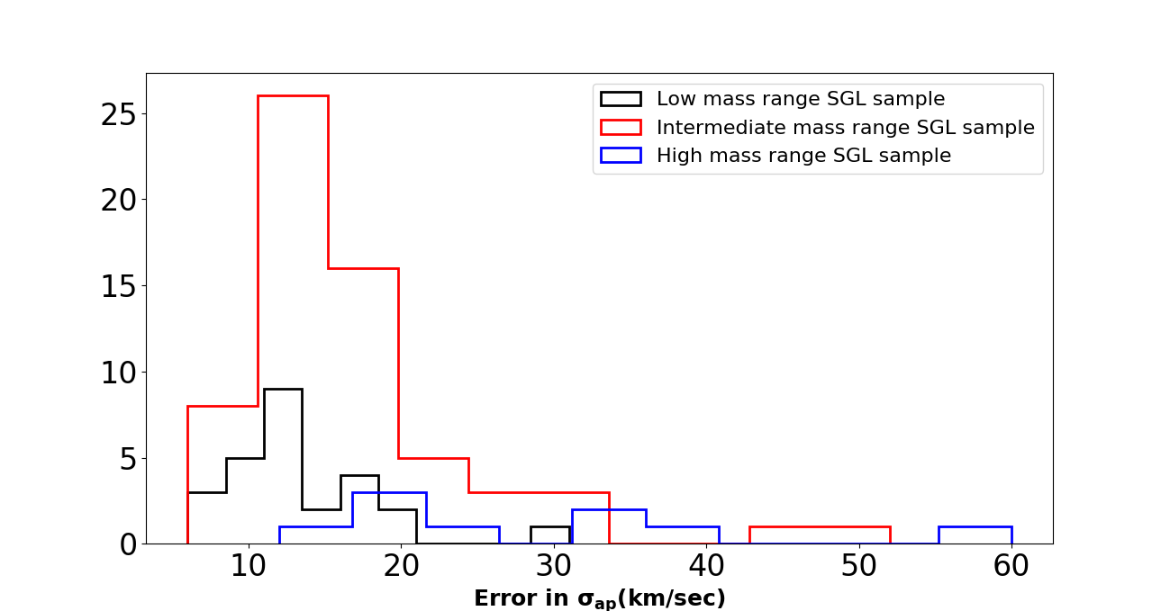
Figure 3: (Left) The distribution of error in $f_{gas}$ for Low, Intermediate, and High mass range sample at $z_{l}$ and $z_{s}$. (Right) The distribution of error in $\sigma_{ap}$ for Low, Intermediate, and High mass range SGL sample.

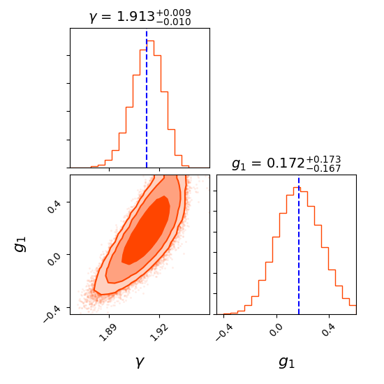
Figure 4: For Low mass range SGL sample: The 1D marginalized likelihood distributions along with 2D marginalized constraints showing the 68%, 95%, and 99% credible regions for the parameters $\gamma$ (from the power law model describing the SGL systems) and $g_{1}$ (from the gas depletion factor $g(z)$), obtained using the Corner python module Foreman-Mackey (2016).

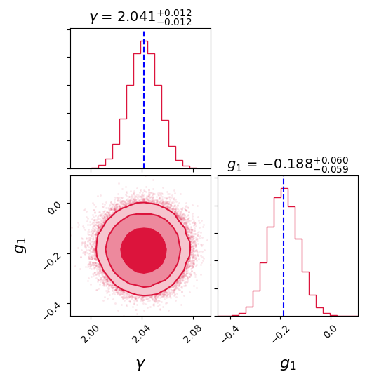
Figure 5: For Intermediate mass range SGL sample: The 1D marginalized likelihood distributions along with 2D marginalized constraints showing the 68%, 95%, and 99% credible regions for the parameters $\gamma$ (from the power law model describing the SGL systems) and $g_{1}$ (from the gas depletion factor $g(z)$), obtained using the Corner python module Foreman-Mackey (2016).

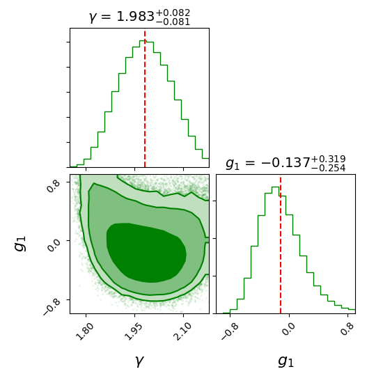
Figure 6: For High mass range SGL sample: The 1D marginalized likelihood distributions along with 2D marginalized constraints showing the 68%, 95%, and 99% credible regions for the parameters $\gamma$ (from the power law model describing the SGL systems) and $g_{1}$ (from the gas depletion factor $g(z)$), obtained using the Corner python module Foreman-Mackey (2016).

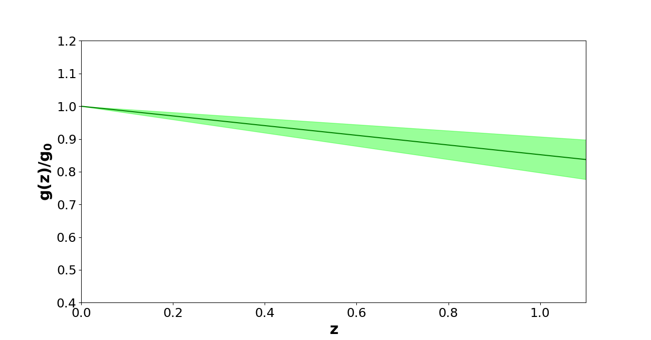
Figure 7: The evolution of the normalized gas depletion factor along with $1\sigma$ error band as a function of redshift using 40 X-ray $f_{gas}$ measurements near $r_{2500}$ from  Mantz et al. (2014). This figure shows a mild evolution of $g(z)$ with respect to redshift.

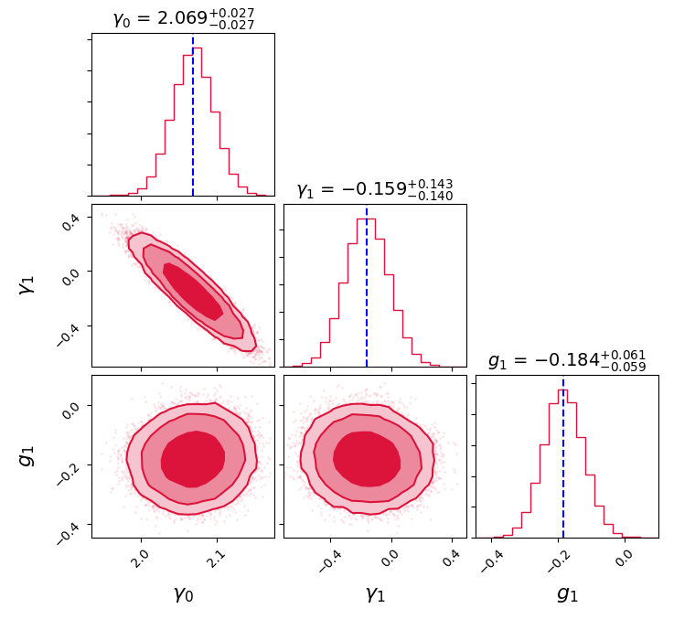
Figure 8: Constraints on $\gamma_{0}$, $\gamma_{1}$, and $g_{1}$ parameters for the Intermediate mass range SGL sample. Here, $\gamma_{1}$ encodes the redshift evolution of $\gamma$. We find only a marginal 1.1$\sigma$ decrease with redshift for $\gamma$.

V Conclusions

In this letter, we have explored a possible time evolution of the gas depletion factor, using a sample of 40 galaxy clusters with their X-ray gas mass fraction obtained in spherical shells at radii near $r_{2500}$. The analyses were performed by using the gas mass fraction measurements in conjunction with sub-samples of strong gravitational lens systems and the cosmic distance duality relation validity. The depletion factor was modelled assuming $g(z)=g_{0}(1+g_{1}z)$, and we found a mild evolution at 2.7$\sigma$, i.e. $g_{1}=-0.15\pm 0.055$ (see Fig. 7). This estimate is obtained by calculating an error-weighted average by combining the different values in Table  1, which contain the results for each of the sub-samples.

In contrast to previous work in this area, our method does not use the Planck constraints on $\Omega_{b}/\Omega_{M}$, although we did assume a flat universe. This is the first work in literature which finds a non-negligible evolution of the gas depletion factor using gas mass fraction measurements in spherical shells at radii near $r_{2500}$. This value is in tension with the results from hydrodynamical simulations. Moreover, our results also reinforce the need for segregating the lenses into low, intermediate and high velocity dispersions, and analyzing them separately. The mass-sheet degeneracy in the gravitational lens system (see Birrer et al. (2016) and references therein) and its effect on our results also could be explored as an interesting extension of this work. blackWe also note that our results are shown for interpolation carried out using GPR. Other reconstruction techniques could change the results somewhat.

It is important to comment that the method discussed here can be used in a near future with data set from the X-ray survey eROSITA Predehl et al. (2021), that is expected to detect $\approx$ 100,000 galaxy clusters, along with followup optical and infrared data from EUCLID mission, Vera Rubin LSST, and Nancy Grace Rowan space telescope, that will discover thousands of strong lensing systems. Then, in the near future, as more and larger data sets with smaller statistical and systematic uncertainties become available, someone will can check the influence of cosmic curvature on our results, given that non-zero curvature has been found in some cosmological analyses Di Valentino et al. (2020).

Appendix

blackHere, we provide a brief introduction to GPR and also compare with other reconstruction techniques such as Artificial Neural Networks (ANN).

GPR: blackGPR is a non-parametric method to interpolate between data points to reconstruct the original function at any input values. It has been widely used in over 200 papers in Cosmology. (See  Seikel et al. (2012); Singirikonda and Desai (2020); Bora and Desai (2021b); Liu et al. (2021b) and references therein for a sampling of some of its applications to Cosmology.) We provide an abridged description of GPR. More details can be found in some of the aforementioned works.

blackThe Gaussian process is characterized by a mean function $\mu(x)$ and a covariance function $cov(f(x),f(\tilde{x}))=k(x,\tilde{x})$, which connects the values of $f$, when evaluated at $x$ and $\tilde{x}$. For a Gaussian kernel, $k(x,\tilde{x})$ can be described by:

$$k(x,\tilde{x})=\sigma_{f}^{2}\exp\left(-\frac{(x-\tilde{x})^{2}}{2l^{2}}\right),$$

where $\sigma_{f}$ and $l$ are the hyperparameters describing the ‘bumpiness’ of the function.

blackFor a set of input points, $\mathbf{X}\equiv x_{i}$, one can generate a vector $\mathbf{f^{*}}$ of function values evaluated at $\mathbf{X^{*}}$ with $f^{*}_{i}=f(x_{i}^{*})$ as

$$\mathbf{f^{*}}=\mathcal{N}(\mathbf{\mu^{*}},K(\mathbf{X^{*},X^{*}}))$$

Here, $\mathcal{N}$ implies that the Gaussian process is evaluated at $x^{*}$, where $f(x^{*})$ is a random value drawn from a normal distribution. Similarly, observational data can be written in as

$$\mathbf{y}=\mathcal{N}(\mathbf{\mu},K(\mathbf{X,X})+C)$$

where $C$ is the covariance matrix of the data. For uncorrelated data, the covariance matrix is simply $diag(\sigma_{i}^{2})$. Using the values of $y$ at $\mathbf{X}$, one can reconstruct $\mathbf{f^{*}}$ using

$$\overline{\mathbf{f^{*}}}=\mathbf{\mu^{*}}+K(\mathbf{X^{*},X})[K(\mathbf{X,X})+C]^{-1}(\mathbf{y-\mu})$$

and

$$cov(\mathbf{f^{*}})=K(\mathbf{X^{*},X^{*}})-K(\mathbf{X^{*},X})[K(\mathbf{X,X})+C]^{-1}K(\mathbf{X,X^{*}})$$

where $\overline{\mathbf{f^{*}}}$ and $cov(\mathbf{f^{*}})$ are mean and covariance of $\mathbf{f^{*}}$ respectively. The diagonal elements of $cov(\mathbf{f^{*}})$ provide us the variance of $\mathbf{f^{*}}$. Our implementation of GPR was implemented using the sklearn package.

ANN: blackANN is another non-parameteric regression technique which has become popular following the increasing usage of Machine Learning applications to Astrophysics Ball and Brunner (2010); Bethapudi and Desai (2018). The ANN consists of an input layer, multiple hidden layers and an output layer. During each layer, a linear transformation is applied to the vector from the previous layer followed by a non-linear activation function, which is then propagated to the next layer. Different choices for the activation function and details of reconstruction using ANN is reviewed in  Liu et al. (2021b). For our analysis we use the publicly available code for ANN based regression in  Wang et al. (2020b). A comparison of $f_{gas}$ reconstruction using both the techniques is illustrated in Fig. 9. We can see that there is a difference in the reconstructed $f_{gas}$ between the two methods.

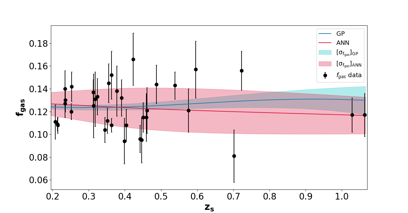
Figure 9: blackA comparison between the Gaussian Processes reconstruction and Artificial Neural Networks (ANN) reconstruction of the gas mass fraction at $z_{s}$ for the Intermediate Mass range sample. The shaded regions show the $1\sigma$ error bars from both the reconstruction techniques.

References

- Mantz et al. (2014) A. B. Mantz, S. W. Allen, R. G. Morris, D. A. Rapetti, D. E. Applegate, P. L. Kelly, A. von der Linden, and R. W. Schmidt, Mon. Not. Roy. Astron. Soc. 440, 2077 (2014), eprint 1402.6212.
- Vikhlinin et al. (2014) A. A. Vikhlinin, A. V. Kravtsov, M. L. Markevich, R. A. Sunyaev, and E. M. Churazov, Physics Uspekhi 57, 317-341 (2014).
- Carbone et al. (2012) C. Carbone, C. Fedeli, L. Moscardini, and A. Cimatti, JCAP 2012, 023 (2012), eprint 1112.4810.
- Desai (2018) S. Desai, Physics Letters B 778, 325 (2018), eprint 1708.06502.
- Sasaki (1996) S. Sasaki, PASJ 48, L119 (1996), eprint astro-ph/9611033.
- Allen et al. (2007) S. W. Allen, D. A. Rapetti, R. W. Schmidt, H. Ebeling, R. G. Morris, and A. C. Fabian, Monthly Notices of the Royal Astronomical Society 383, 879 (2007).
- Ettori et al. (2009) S. Ettori, A. Morandi, P. Tozzi, I. Balestra, S. Borgani, P. Rosati, L. Lovisari, and F. Terenziani, Astron. & Astrophys. 501, 61 (2009), eprint 0904.2740.
- Pen (1997) U.-L. Pen, New Astronomy 2, 309 (1997), eprint astro-ph/9610090.
- White et al. (1993) S. D. M. White, J. F. Navarro, A. E. Evrard, and C. S. Frenk, Nature (London) 366, 429 (1993).
- Planelles et al. (2013) S. Planelles, S. Borgani, K. Dolag, S. Ettori, D. Fabjan, G. Murante, and L. Tornatore, Mon. Not. R. Astron. Soc. 431, 1487 (2013), eprint 1209.5058.
- Battaglia et al. (2013) N. Battaglia, J. R. Bond, C. Pfrommer, and J. L. Sievers, Astrophys. J. 777, 123 (2013), eprint 1209.4082.
- Bora and Desai (2021a) K. Bora and S. Desai, European Physical Journal C 81, 296 (2021a), eprint 2103.12695.
- Le Brun et al. (2017) A. M. C. Le Brun, I. G. McCarthy, J. Schaye, and T. J. Ponman, Mon. Not. R. Astron. Soc. 466, 4442 (2017), eprint 1606.04545.
- Kaiser (1986) N. Kaiser, Mon. Not. R. Astron. Soc. 222, 323 (1986).
- Mohr et al. (1999) J. J. Mohr, B. Mathiesen, and A. E. Evrard, Astrophys. J. 517, 627 (1999), eprint astro-ph/9901281.
- Holanda et al. (2017) R. F. L. Holanda, V. C. Busti, J. E. Gonzalez, F. Andrade-Santos, and J. S. Alcaniz, JCAP 2017, 016 (2017), eprint 1706.07321.
- Planck Collaboration et al. (2016) Planck Collaboration, P. A. R. Ade, N. Aghanim, M. Arnaud, M. Ashdown, J. Aumont, C. Baccigalupi, A. J. Banday, R. B. Barreiro, J. G. Bartlett, et al., Astron. & Astrophys. 594, A13 (2016), eprint 1502.01589.
- Ellis (2007) G. F. R. Ellis, General Relativity and Gravitation 39, 1047 (2007).
- Holanda (2018) R. F. L. Holanda, Astroparticle Physics 99, 1 (2018), eprint 1711.05173.
- LaRoque et al. (2006) S. J. LaRoque, M. Bonamente, J. E. Carlstrom, M. K. Joy, D. Nagai, E. D. Reese, and K. S. Dawson, Astrophys. J. 652, 917 (2006), eprint astro-ph/0604039.
- Zheng et al. (2019) X. Zheng, J.-Z. Qi, S. Cao, T. Liu, M. Biesiada, S. Miernik, and Z.-H. Zhu, European Physical Journal C 79, 637 (2019), eprint 1907.06509.
- Hilton et al. (2018) M. Hilton, M. Hasselfield, C. Sifón, N. Battaglia, S. Aiola, V. Bharadwaj, J. R. Bond, S. K. Choi, D. Crichton, R. Datta, et al., Astrophys. J. Suppl. Ser. 235, 20 (2018), eprint 1709.05600.
- Jimenez and Loeb (2002) R. Jimenez and A. Loeb, Astrophys. J. 573, 37 (2002), eprint astro-ph/0106145.
- Chiu et al. (2018) I. Chiu, J. J. Mohr, M. McDonald, S. Bocquet, S. Desai, M. Klein, H. Israel, M. L. N. Ashby, A. Stanford, B. A. Benson, et al., Mon. Not. R. Astron. Soc. 478, 3072 (2018), eprint 1711.00917.
- Planck Collaboration et al. (2011) Planck Collaboration, P. A. R. Ade, N. Aghanim, M. Arnaud, M. Ashdown, J. Aumont, C. Baccigalupi, A. Balbi, A. J. Banday, R. B. Barreiro, et al., Astron. & Astrophys. 536, A8 (2011), eprint 1101.2024.
- Planck Collaboration et al. (2020) Planck Collaboration, N. Aghanim, Y. Akrami, M. Ashdown, J. Aumont, C. Baccigalupi, M. Ballardini, A. J. Banday, R. B. Barreiro, N. Bartolo, et al., Astron. & Astrophys. 641, A6 (2020), eprint 1807.06209.
- Leaf and Melia (2018) K. Leaf and F. Melia, Mon. Not. Roy. Astron. Soc. 478, 5104 (2018), eprint 1805.08640.
- Schneider et al. (1992) P. Schneider, J. Ehlers, and E. E. Falco, Gravitational Lenses (1992).
- Bartelmann (2010) M. Bartelmann, Classical and Quantum Gravity 27, 233001 (2010), eprint 1010.3829.
- Kumar et al. (2021) D. Kumar, D. Jain, S. Mahajan, A. Mukherjee, and N. Rani, Phys. Rev. D 103, 063511 (2021), eprint 2002.06354.
- Wei et al. (2022) J.-J. Wei, Y. Chen, S. Cao, and X.-F. Wu, Astrophys. J. Lett. 927, L1 (2022), eprint 2202.07860.
- Wang et al. (2020a) B. Wang, J.-Z. Qi, J.-F. Zhang, and X. Zhang, Astrophys. J. 898, 100 (2020a), eprint 1910.12173.
- Cao et al. (2017) S. Cao, X. Li, M. Biesiada, T. Xu, Y. Cai, and Z.-H. Zhu, Astrophys. J. 835, 92 (2017), eprint 1701.00357.
- Liu et al. (2021a) T. Liu, S. Cao, M. Biesiada, Y. Liu, Y. Lian, and Y. Zhang, Mon. Not. R. Astron. Soc. 506, 2181 (2021a), eprint 2106.15145.
- Colaço et al. (2021) L. R. Colaço, R. F. L. Holanda, and R. Silva, European Physical Journal C 81, 822 (2021), eprint 2004.08484.
- Qi et al. (2021) J.-Z. Qi, J.-W. Zhao, S. Cao, M. Biesiada, and Y. Liu, Mon. Not. R. Astron. Soc. 503, 2179 (2021), eprint 2011.00713.
- Cao et al. (2019) S. Cao, J. Qi, Z. Cao, M. Biesiada, J. Li, Y. Pan, and Z.-H. Zhu, Scientific Reports 9, 11608 (2019), eprint 1910.10365.
- Futamase and Yoshida (2001) T. Futamase and S. Yoshida, Progress of Theoretical Physics 105, 887 (2001), eprint gr-qc/0011083.
- Biesiada (2006) M. Biesiada, Phys. Rev. D 73, 023006 (2006).
- Grillo et al. (2008) C. Grillo, M. Lombardi, and G. Bertin, Astron. & Astrophys. 477, 397 (2008), eprint 0711.0882.
- Cao et al. (2012) S. Cao, G. Covone, and Z.-H. Zhu, Astrophys. J. 755, 31 (2012), eprint 1206.4948.
- Cao et al. (2015) S. Cao, M. Biesiada, R. Gavazzi, A. Piórkowska, and Z.-H. Zhu, Astrophys. J. 806, 185 (2015), eprint 1509.07649.
- Holanda et al. (2017a) R. F. L. Holanda, V. C. Busti, F. S. Lima, and J. S. Alcaniz, JCAP 09, 039 (2017a), eprint 1611.09426.
- Cao et al. (2018) S. Cao, J. Qi, M. Biesiada, X. Zheng, T. Xu, and Z.-H. Zhu, The Astrophysical Journal 867, 50 (2018).
- Amante et al. (2020) M. H. Amante, J. Magaña, V. Motta, M. A. García-Aspeitia, and T. Verdugo, Mon. Not. Roy. Astron. Soc. 498, 6013 (2020), eprint 1906.04107.
- Lizardo et al. (2021) A. Lizardo, M. H. Amante, M. A. García-Aspeitia, J. Magaña, and V. Motta, Mon. Not. R. Astron. Soc. 507, 5720 (2021), eprint 2008.10655.
- Bora et al. (2021) K. Bora, R. F. L. Holanda, and S. Desai, European Physical Journal C 81, 596 (2021), eprint 2105.02168.
- Liao (2019) K. Liao, Astrophys. J. 885, 70 (2019), eprint 1906.09588.
- Applegate et al. (2016) D. E. Applegate, A. Mantz, S. W. Allen, A. von der Linden, R. G. Morris, S. Hilbert, P. L. Kelly, D. L. Burke, H. Ebeling, D. A. Rapetti, et al., Mon. Not. R. Astron. Soc. 457, 1522 (2016), eprint 1509.02162.
- Gonçalves et al. (2012) R. S. Gonçalves, R. F. L. Holanda, and J. S. Alcaniz, Mon. Not. R. Astron. Soc. 420, L43 (2012), eprint 1109.2790.
- Holanda et al. (2022) R. F. L. Holanda, F. S. Lima, A. Rana, and D. Jain, European Physical Journal C 82, 115 (2022), eprint 2104.01614.
- Bora and Desai (2021b) K. Bora and S. Desai, JCAP 2021, 052 (2021b), eprint 2104.00974.
- Holanda et al. (2017b) R. F. L. Holanda, V. C. Busti, J. E. Gonzalez, F. Andrade-Santos, and J. S. Alcaniz, JCAP 12, 016 (2017b), eprint 1706.07321.
- Mantz et al. (2022) A. B. Mantz, R. G. Morris, S. W. Allen, R. E. A. Canning, L. Baumont, B. Benson, L. E. Bleem, S. R. Ehlert, B. Floyd, R. Herbonnet, et al., Mon. Not. R. Astron. Soc. 510, 131 (2022), eprint 2111.09343.
- Mantz et al. (2015) A. B. Mantz, S. W. Allen, R. G. Morris, R. W. Schmidt, A. von der Linden, and O. Urban, Mon. Not. R. Astron. Soc. 449, 199 (2015), eprint 1502.06020.
- Mantz et al. (2016) A. B. Mantz, S. W. Allen, R. G. Morris, and R. W. Schmidt, Mon. Not. R. Astron. Soc. 456, 4020 (2016), eprint 1509.01322.
- Cao et al. (2016a) S. Cao, M. Biesiada, X. Zheng, and Z.-H. Zhu, Mon. Not. R. Astron. Soc. 457, 281 (2016a), eprint 1601.00409.
- Cao and Zhu (2011) S. Cao and Z. Zhu, Science China Physics, Mechanics, and Astronomy 54, 2260 (2011), eprint 1102.2750.
- Chen et al. (2019) Y. Chen, R. Li, Y. Shu, and X. Cao, Mon. Not. R. Astron. Soc. 488, 3745 (2019), eprint 1809.09845.
- Shu et al. (2017) Y. Shu, J. R. Brownstein, A. S. Bolton, L. V. E. Koopmans, T. Treu, A. D. Montero-Dorta, M. W. Auger, O. Czoske, R. Gavazzi, P. J. Marshall, et al., Astrophys. J. 851, 48 (2017), eprint 1711.00072.
- Koopmans et al. (2009) L. V. E. Koopmans, A. Bolton, T. Treu, O. Czoske, M. W. Auger, M. Barnabè, S. Vegetti, R. Gavazzi, L. A. Moustakas, and S. Burles, Astrophys. J. Lett. 703, L51 (2009), eprint 0906.1349.
- Auger et al. (2010) M. W. Auger, T. Treu, A. S. Bolton, R. Gavazzi, L. V. E. Koopmans, P. J. Marshall, L. A. Moustakas, and S. Burles, The Astrophysical Journal 724, 511 (2010).
- Barnabè et al. (2011) M. Barnabè, O. Czoske, L. V. E. Koopmans, T. Treu, and A. S. Bolton, Mon. Not. R. Astron. Soc. 415, 2215 (2011), eprint 1102.2261.
- Sonnenfeld et al. (2013) A. Sonnenfeld, T. Treu, R. Gavazzi, S. H. Suyu, P. J. Marshall, M. W. Auger, and C. Nipoti, Astrophys. J. 777, 98 (2013), eprint 1307.4759.
- Cao et al. (2016b) S. Cao, M. Biesiada, M. Yao, and Z.-H. Zhu, Mon. Not. R. Astron. Soc. 461, 2192 (2016b), eprint 1604.05625.
- Holanda et al. (2017) R. F. L. Holanda, S. H. Pereira, and D. Jain, Mon. Not. R. Astron. Soc. 471, 3079 (2017), eprint 1705.06622.
- Seikel et al. (2012) M. Seikel, C. Clarkson, and M. Smith, JCAP 2012, 036 (2012), eprint 1204.2832.
- Singirikonda and Desai (2020) H. Singirikonda and S. Desai, European Physical Journal C 80, 694 (2020), eprint 2003.00494.
- Foreman-Mackey et al. (2013) D. Foreman-Mackey, D. W. Hogg, D. Lang, and J. Goodman, PASP 125, 306 (2013), eprint 1202.3665.
- Foreman-Mackey (2016) D. Foreman-Mackey, The Journal of Open Source Software 1, 24 (2016).
- Birrer et al. (2016) S. Birrer, A. Amara, and A. Refregier, JCAP 2016, 020 (2016), eprint 1511.03662.
- Predehl et al. (2021) P. Predehl, R. Andritschke, V. Arefiev, V. Babyshkin, O. Batanov, W. Becker, H. Böhringer, A. Bogomolov, T. Boller, K. Borm, et al., Astron. & Astrophys. 647, A1 (2021), eprint 2010.03477.
- Di Valentino et al. (2020) E. Di Valentino, A. Melchiorri, and J. Silk, Nature Astronomy 4, 196 (2020), eprint 1911.02087.
- Liu et al. (2021b) T. Liu, S. Cao, S. Zhang, X. Gong, W. Guo, and C. Zheng, European Physical Journal C 81, 903 (2021b), eprint 2110.00927.
- Ball and Brunner (2010) N. M. Ball and R. J. Brunner, International Journal of Modern Physics D 19, 1049 (2010), eprint 0906.2173.
- Bethapudi and Desai (2018) S. Bethapudi and S. Desai, Astronomy and Computing 23, 15 (2018), eprint 1704.04659.
- Wang et al. (2020b) G.-J. Wang, S.-Y. Li, and J.-Q. Xia, Astrophys. J. Suppl. Ser. 249, 25 (2020b), eprint 2005.07089.