Building diquark model from Lattice QCD

Abstract

A novel Lattice QCD (LQCD) method to determine the quark-diquark ($q$-$D$) interaction potential together with the diquark mass ($m_{D}$) is proposed. Similar to the HAL QCD method, $q$-$D$ potential is determined by demanding it to reproduce the $q$-$D$ equal-time Nambu-Bethe-Salpeter (NBS) wave function. To do this, it is necessary to use the masses of the quark and the diquark as inputs, which however are not straightforwardly obtained because of the color confinement of QCD. In this work, masses of quark and diquark are determined by demanding that the p-wave spectrums from the two-point correlators be reproduced by the potentials for $c\bar{c}$ and $q$-$D$ sectors determined from the NBS wave functions. Numerical calculations are performed by using 2+1 flavor QCD gauge configurations with the pion mass $m_{\pi}\simeq 700$ MeV generated by PACS-CS collaboration. We apply our method to the $c$-$\bar{c}$ system and the charm-diquark system ($\Lambda_{c}$ baryon) to obtain the charm quark mass, diquark mass and the $c$-$D$ potential. Our preliminary analysis leads to the diquark mass $m_{D}\simeq 1.127$ GeV which is roughly consistent with a naive estimate based on the constituent quark picture, i.e., $m_{D}\simeq m_{\rho}\simeq 1.12$ GeV and $m_{D}\simeq 2m_{N}/3\simeq 1.06$ GeV.

1 Introduction

Solving quark many-body problems and revealing the hadron structures are important themes in hadron physics. In general, the computational complexity is a problem in solving quantum many-body systems and approximations are often used. One example of such an approximation is to reduce the degrees of freedom by introducing a virtual bound state of the particles constituting the system. The diquark, which is a virtual bound state of two quarks, is a typical example. By introducing a diquark, a baryon can be expressed as a quark-diquark ($q$-$D$) bound state. A model based on the idea of diquarks are called the diquark model and has been widely used to provide predictions on hadron structures and energy levelsjaffe .

Since diquarks are color-charged objects, they cannot be observed due to the color confinement in the quantum chromodynamics (QCD). Because of this limitation, the parameters in the diquark model such as the $q$-$D$ interaction and the diquark mass have so far been determined on the basis of simplified phenomenologymauro . Therefore, determining these quantities faithfully to QCD is indispensable for the development of hadron physics.

There have been several studies on diquarks from lattice QCD (LQCD) Monte Carlo calculation, the first-principles calculations of QCD. Namely, Ref.diquark_mass calculated the gauge-dependent diquark correlation function and obtained the diquark mass in the Landau gauge. To avoid such a gauge-dependence, Ref.diquark_size proposed a method to consider the diquark correlation function in the presence of an infinitely heavy static quark which is introduced to neutralize the system. However, though this method is gauge-independent, the dynamics of the diquark differ from that in the experimentally observed hadrons due to the introduction of the static quark.

Recently, a method to determine the quark-antiquark ($q$-$\bar{q}$) interaction potential from LQCD was proposed by Ikeda and IidaIkeda-Iida . In their method, the potential that appears in the interaction term of the Schrödinger equation is determined by demanding it to reproduce the equal-time NBS wave function and its energy. The $q$-$\bar{q}$ potential calculated by Ikeda and Iida is qualitatively similar to the phenomenologically determined Cornell-type potentialkinoshita . However, Ikeda-Iida employed a very naive estimate of the quark mass which is half the vector meson mass. To improve this point, Kawanai and SasakiKawanai-Sasaki proposed a method to determine the quark mass by demanding the spin-spin interaction potential to vanish at the long distance. The potential and mass determined in this way reproduce the energy levels of mesons with satisfactory accuracyKawanai-Sasaki2 .

These methods of determining the potential and the mass using the NBS wave function calculated by LQCD seems to be promising. However, the Kawanai-Sasaki method does not work for quark-diquark systems where the diquark is the scalar-diquark because of the absence of the spin-spin interaction potential. Note that the scalar-diquark is considered as the most relevant diquark in the hadronic phenomenology. In this study, we propose an alternative method to determine the diquark mass. We determine the $q$-$D$ potential by demanding it to reproduce the equal-time NBS wave function. The diquark mass is determined by demanding this $q$-$D$ potential to reproduce the p-wave excitation energy of the $q$-$D$ system.

This paper is organized as follows. The first section is dedicated to the formulation of our method. The NBS wave function is defined. The Schrödinger equation is used to obtain the diquark mass and the $q$-$D$ potential. To be specific, we focus on the $\Lambda_{c}$ baryon consisting of a spectator charm quark and a scalar [$ud$] diquark; $J^{P}=0^{+}$, isospin $I=0$ and color $\boldmath{\bar{3}}$. In the second section, the LQCD setup is explained. In the third section, we show the numerical results for the NBS wave function, the diquark mass and the potential. Finally in the last section, we summarize our work.

2 Formalism

We start from the equal-time NBS wave function in the rest frame given by

$$\psi_{\Lambda(J^{P})}(\bm{r})\equiv\left\langle 0\left|D_{c}(\bm{r})c_{c}(\bm{0})\right|\Lambda_{c}(J^{P})\right\rangle,$$ (1)

where $|\Lambda_{c}(J^{P})\rangle$ denotes the $\Lambda_{c}$ baryon state for $J^{P}$ sector. $c_{c}(\bm{x})$ and $D_{c}(\bm{x})\equiv\varepsilon_{abc}u_{a}^{T}(\bm{x})C\gamma_{5}d_{b}(\bm{x})$ denote the field operators for the charm quark and the composite diquark, respectively. $u_{a}(\bm{x})$, $d_{a}(\bm{x})$ denote the field operators for the up and the down quarks, respectively, with $C$ being the charge conjugation matrix. $a$,$b$ and $c$ are the color indices. The Levi-Civita symbol $\varepsilon_{abc}$ is introduced to make the color representations of the diquark operator to be $\bar{\bm{3}}$. To obtain the NBS wave function, we consider the $c$-$D$ four-point correlator $C(\bm{x}-\bm{y},t)\equiv\langle 0|T\{D_{c}(\bm{x},t)c_{c}(\bm{y},t)\cdot{\mathcal{J}}_{\Lambda(J^{P})}(t=0)\}|0\rangle$ with $\mathcal{J}_{\Lambda(J^{P})}$ being the wall source operator for the $\Lambda(J^{P})$ baryon in our calculation. The NBS wave function is obtained in the large $t$ region of $C(\bm{r},t)$ as $C(\bm{r},t)\simeq\psi_{\Lambda(J^{P})}(\bm{r})\cdot A\exp\left(-M_{\Lambda(J^{P})}t\right)$ with $A\equiv\langle\Lambda_{J^{P}}|{\mathcal{J}}_{J^{P}}|0\rangle$.

We define the quark-diquark potential $\hat{U}$ by demanding that the following Schrödinger equation be satisfied by the equal-time NBS wave function as

$$\left(-\frac{\nabla^{2}}{2\mu_{cD}}+\hat{U}\right)\psi_{\Lambda(J^{P})}(\bm{r})=E_{\Lambda(J^{P})}\psi_{\Lambda(J^{P})}(\bm{r}),$$ (2)

where $\mu_{cD}\equiv m_{c}m_{D}/(m_{c}+m_{D})$ denotes the reduced mass of the system with $m_{c}$ and $m_{D}$ being the masses of charm quark and the diquark respectively. We treat these masses as unknown parameters at this point, which will be determined later. $E_{\Lambda(J^{P})}\equiv M_{\Lambda(J^{P})}-(m_{c}+m_{D})$ denotes the binding energy with $M_{\Lambda(J^{P})}$ being the mass of $\Lambda_{c}$ baryon for $J^{P}$ channel. We apply the derivative expansion to $\hat{U}$ as

$$\hat{U}=U_{0}(r)+U_{\rm LS}(r)\bm{L}\cdot\bm{s}+O(\nabla^{2}),$$ (3)

where $U_{0}(r)$, $U_{\rm LS}(r)$, $\bm{L}$ and $\bm{s}$ denote the central and the spin-orbit potentials, the orbital angular momentum operator and the spin operator of the charm quark, respectively.

To proceed, we define the following quantity:

$$\widetilde{U}(\bm{r})\equiv\frac{\nabla^{2}\psi_{\Lambda(1/2^{+})}(\bm{r})}{\psi_{\Lambda(1/2^{+})}(\bm{r})}\simeq 2\mu_{cD}\left(U_{0}(\bm{r})-E_{\Lambda(1/2^{+})}\right),$$ (4)

which we refer to as the pre-potential. Due to Eq. (2), NBS wave functions for $J^{P}=1/2^{-},3/2^{-}$ satisfy the following pre-Schrödinger equation:

$$\left(-\nabla^{2}+\widetilde{U}(\bm{r})+2\mu_{cD}U_{\rm LS}(\bm{r})\bm{L}\cdot\bm{s}\right)\psi_{\Lambda(J^{P})}(\bm{r})=2\mu_{cD}\left(M_{\Lambda(J^{P})}-M_{\Lambda(1/2^{+})}\right)\psi_{\Lambda(J^{P})}(\bm{r}).$$ (5)

By treating the spin-orbit potential $U_{\rm LS}(r)\bm{L}\cdot\bm{s}$ as a perturbation, the pre-Schrödinger equations are solved in $J^{P}=1/2^{-}$ and $3/2^{-}$ sectors to have

$$\widetilde{E}_{\rm PW}-2\mu_{cD}\left\langle U_{\rm LS}\right\rangle \simeq 2\mu_{cD}\left(M_{\Lambda(1/2-)}-M_{\Lambda(1/2+)}\right)$$ (6)

$$\widetilde{E}_{\rm PW}+\mu_{cD}\left\langle U_{\rm LS}\right\rangle \simeq 2\mu_{cD}\left(M_{\Lambda(3/2-)}-M_{\Lambda(1/2+)}\right),$$

where $\widetilde{E}_{\rm PW}$ denotes the degenerate unperturbed pre-energy for the p-wave sector which is obtained by solving the unperturbed pre-Schrödinger equation

$$\left(-\nabla^{2}+\widetilde{U}(\rm r)\right)\psi(\bm{r})=\widetilde{E}\psi(\bm{r}),$$ (7)

in the p-wave sector. By eliminating $\langle U_{\rm LS}\rangle$ from these two equations, we have

$$\mu_{cD}=\frac{3}{2}\frac{\widetilde{E}_{\rm PW}}{M_{\Lambda(1/2-)}+2M_{\Lambda(3/2-)}-3M_{\Lambda(1/2+)}},$$ (8)

which enables us to determine the reduced mass by using $M_{\Lambda(J^{P})}$ obtained from the two-point correlators. The diquark mass $m_{D}$ can be obtained by combining the charm quark mass $m_{c}$ which can be obtained by applying a similar method to $c\bar{c}$ sector. Finally, the quark-diquark potential is obtained from the pre-potential as

$$U_{0}(\bm{r})=\frac{1}{2\mu_{cD}}\widetilde{U}_{\Lambda(1/2^{+})}(\bm{r})+M_{\Lambda(1/2^{+})}-m_{D}-m_{c}.$$ (9)

3 LQCD setup

In this work, we use 2+1 flavor QCD gauge configurations generated by PACS-CS Collaboration on $32^{3}\times 64$ lattice pacs_config , which employs the RG improved Iwasaki gauge action at $\beta=1.9$ iwasaki1 and the non-perturbatively $O(a)$ improved Wilson quark action at $(\kappa_{\rm ud},\kappa_{\rm s})=(0.13700,0.13640)$ and $C_{\rm SW}=1.715$ cl_wilson . This parameter set leads to the lattice spacing $a=0.0907(13)$ fm ($a^{-1}\simeq 2.175$ GeV), the spatial extent $L=32a\simeq 2.9$ fm, the pion mass $m_{\pi}\simeq 700$ MeV and the nucleon mass $m_{N}\simeq 1584$ MeV. For the charm quark, the relativistic heavy quark action (RHQ) is used in order to reduce the systematic errors originating from the heavy charm quark mass RHQ_on_LQCD . We use the same parameter set as given in Ref.namekawa . The lattice QCD calculation is carried out by using 399 gauge configurations for several different source points for better statistics. The statistical errors are evaluated by using the Jackknife prescription. We employ the Coulomb gauge fixing though out the calculations.

4 Numerical results

Fig.1 shows the NBS wave function for $\Lambda_{c}(1/2^{+})$ extracted from the $c$-$D$ four-point correlation function at time-slice $t/a=15$. Note that $t/a=15$ is the smallest time-slice in the plateau region.

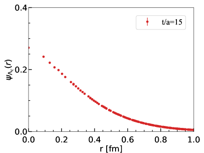
Figure 1: $c$-$D$ NBS wave function of the $\Lambda_{c}(\frac{1}{2}^{+})$ state. The NBS wave function is extracted from the four-point function at $t/a=15$. The NBS wave function is normalized by using $L^{2}$-norm.

Fig.2 shows the result of the pre-potential Eq. (4) together with the result of the fit with the Cornell-plus-log type fit function

$$V^{{\rm fit}}(r)=-A/r+Br+C\log(r/a)+{\rm const}.$$ (10)

The log term is introduced to improve the quality of the fit. In the $q$-$\bar{q}$ sector, it is suggested that such log term may appear due to the finite quark mass effect Koma_Koma . To avoid an artifact from the spatial boundary condition, we perform the fit in a restricted region $0<r/a\leq 10$.

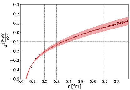
Figure 2: $c$-$D$ pre-potential (black dots) and the result of the fit with the Cornell-plus-log function(red line). The shaded area denotes the statistical error.

Next, we use the fitted pre-potential to solve Eq. (7) to obtain the p-wave excitation pre-energy $\widetilde{E}_{\rm PW}$. To solve the equation numerically, we employ the Discretized Variable Representation (DVR) method often used in quantum chemistry DVR1 . We obtain $\widetilde{E}_{\rm PW}=0.641(4)$ GeV². The results for s-wave and p-wave solutions are shown in Fig.3. We see a good agreement between the LQCD data and the numerical solution for the s-wave.

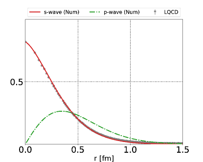
Figure 3: Numerical solutions for s-wave (red solid line) and p-wave (green dotted line) obtained from the pre-potential. The LQCD data (star) is also shown for comparison. The NBS wave function is normalized accordingly.

We calculate the two-point correlators to obtain the masses $M_{\Lambda(1/2^{+})}$, $M_{\Lambda(1/2^{-})}$ and $M_{\Lambda(3/2^{-})}$ of $\Lambda_{c}$ baryons. The results are summarized in Table 1.

Table 1: The energy levels of $\Lambda_{c}$ baryons.

$\frac{1}{2}^{+}$	$\frac{1}{2}^{-}$	$\frac{3}{2}^{-}$
2.684(4) GeV	3.083(81) GeV	3.176(12) GeV

The reduced mass $\mu_{cD}$ is now calculated by using Eq. (8). Combining $\mu_{cD}$ and the charm quark mass $m_{c}=1.823(19)$ GeV obtained by applying the similar procedure to the $c$-$\bar{c}$ sector, the diquark mass is obtained as $m_{D}=1.127(114)$ GeV. Now the $c$-$D$ potential is obtained by using Eq. (9). Note that our diquark mass is roughly consistent with a naive estimate based on the constituent quark picture, i.e., $m_{D}\simeq m_{\rho}\simeq 1.12$ GeV and $m_{D}\simeq 2m_{N}/3\simeq 1.06$ GeV. We make a comment. In Fig.1 and Fig.2, we recognize that the lattice QCD data of the NBS wave function and the pre-potential deviate from a single-valued function of $r$ at short distance, which seems to be due to the discretization artifact of lattice Coulomb gauge. As a result, the fit of the pre-potential at short distance receives an uncertainty, which may lead to a systematic uncertainty of a few hundred MeV of the diquark mass. There is a similar problem in the $q\bar{q}$ sector, which may lead to an uncertainty of a few hundred MeV in the determination of the charm quark mass. To improve, careful analysis is needed.

5 Sammary

We have proposed a novel method to obtain the diquark mass and the quark-diquark interaction potential from LQCD. By using 2+1 flavor QCD gauge configurations generated by PACS-CS collaboration with $m_{\pi}\simeq 700$ MeV, we have performed a lattice QCD Monte Carlo calculation. A preliminary analysis has lead to the diquark mass $m_{D}=1.127(114)$ GeV, which is consistent with a naive estimate based on the constituent quark picture, i.e., $m_{D}\simeq m_{\rho}\simeq 1.12$ GeV and $m_{D}\simeq 2m_{N}/3\simeq 1.06$ GeV. We have obtained a quark-diquark potential which is qualitatively similar to the well-known Cornell type potential.

- (1) R. Jaffe, Physics Reports 409(1), 1 (2005)
- (2) M. Anselmino, E. Predazzi, S. Ekelin, S. Fredriksson, D.B. Lichtenberg, Rev. Mod. Phys. 65, 1199 (1993)
- (3) M. Hess, F. Karsch, E. Laermann, I. Wetzorke, Phys. Rev. D 58, 111502 (1998)
- (4) C. Alexandrou, P. de Forcrand, B. Lucini, Phys. Rev. Lett. 97, 222002 (2006)
- (5) Y. Ikeda, H. Iida, Progress of Theoretical Physics 128(5), 941 (2012)
- (6) E. Eichten, et al., Phys. Rev. Lett. 34, 369 (1975)
- (7) T. Kawanai, S. Sasaki, Phys. Rev. Lett. 107, 091601 (2011)
- (8) T. Kawanai, S. Sasaki, Phys. Rev. D 92, 094503 (2015)
- (9) S. Aoki, et al., Phys. Rev. D 79, 034503 (2009)
- (10) Y. Iwasaki. unpublished (2011)
- (11) S. Aoki, M. Fukugita, S. Hashimoto, K.I. Ishikawa, N. Ishizuka, Y. Iwasaki, K. Kanaya, T. Kaneko, Y. Kuramashi, M. Okawa, S. Takeda, Y. Taniguchi, N. Tsutsui, A. Ukawa, N. Yamada, T. Yoshié, Phys. Rev. D 73, 034501 (2006)
- (12) S. Aoki, et al., Progress of Theoretical Physics 109(3), 383 (2003)
- (13) Y. Namekawa, et al., Phys. Rev. D 84, 074505 (2011)
- (14) Y. Koma, M. Koma, Few-Body Systems 54 (2013)
- (15) D.T. Colbert, W.H. Miller, The Journal of Chemical Physics 96(3), 1982 (1992)
- (16) M.G. Beckett, P. Coddington, B. Joó, C.M. Maynard, D. Pleiter, O. Tatebe, T. Yoshie, Computer Physics Communications 182(6), 1208 (2011)
- (17) International Lattice Data Grid (ILDG). http://www.lqcd.org/ildg
- (18) Japan Lattice Data Grid (JLDG). http://www.jldg.org
- (19) Lattice QCD code Bridge++. http://bridge.kek.jp/Lattice-code/