Spinor-Vector Duality and BSM Phenomenology

Abstract

Spinor–Vector Duality (SVD) has been observed in worldsheet constructions of heterotic–string compactifications. Recently, its realisation in the effective field theory limit of string vacua in six and five dimensions has been investigated. The SVD has been used to construct a string model that allows for an extra family universal $U(1)$, with the standard $E_{6}$ embedding of its charges, to remain unbroken down to low scales. Anomaly cancellation of the extra $U(1)$ charges mandates the existence of additional matter states at the extra $U(1)$ breaking scale, which affects precision measurements of Standard Model parameters. I discuss the construction of non-supersymmetric sting vacua and “modular maps” akin to the spacetime supersymmetry map. Such “modular maps” provide a glimpse into the enormous symmetry structure underlying the entire space of perturbative string vacua that is yet to be uncovered.

1 Introduction

The Standard Model of particle physics successfully accounts for most of the observable data to date. The Standard Model is not the end of the road. In the first place it contains too many parameters. In the Standard Model itself we may count the 45 gauge charges; the 9 fermion masses and 4 CKM parameters; the 3 gauge couplings; the Higgs VEV and coupling; and the strong CPX parameter; for a total of 45+19= 64 parameters. If one adds neutrino charges and masses to the melee, as indicated by experiments, the counting grows further. One often hears that physicists crave evidence for physics beyond the Standard Model. If those came in the form of new forces and new particles that would entail increasing the number of parameters required to account for observations. An alternative approach is to reduce the number of free parameters by refining the mathematical models. Grand Unified Theories (GUTs) make a step in that direction by embedding the Standard Model states in multiplets of the grand unification group. Most appealing in this regard is the embedding in $SO(10)$ GUT in which the fermion multiplets are embedded in three spinorial 16 representations of $SO(10)$. Hence, the number of gauge charge parameters is reduced from $3\times 3\times 6=54$ to one, being the number of 16 representations required to embed the Standard Model states, plus right–handed neutrinos. Grand Unified Theories, however, cannot be the end of the road either. There are still too many ad hoc parameters, in particular in the flavour sector. The origin of the basic flavour structure, the duplication of the family multiplets and the parameters that determine their masses and mixing, can only be sought by embedding the Standard Model in a theory of quantum gravity.

Recently, experimental evidence for physics beyond the Standard Model has been in the news, generating substantial excitement LHCbExp ; gminus2 . It should be stated that the merit and value of these, and other experiments, is not in providing evidence for physics beyond the Standard Model. Their value and merit is in reducing the error bars of the measurements of the basic experimental observables. The marvel of the experiments is in the design, construction and delivery of the specified experimental targets in energy, luminosity, and other variables. If an experiment is able to reduce the experimental uncertainty of the basic observable parameters, then it is celebrated as great success and triumph of human curiosity and ingenuity. Whether or not it discovers physics beyond the Standard Model is not a measure of its success. One can go further and propose that experimentalists should not care at all about physics beyond the Standard Model. All experimentalists have to do is to improve the measurements of the Standard Model parameters. If physics beyond the Standard Model exists it will appear as an inconsistency in using the Standard Model parameters to paramatrise the observable data.

String theory provides a self consistent framework to explore the embedding of the Standard Model in quantum gravity. Its consistency conditions dictate the existence of the gauge, matter and scalar sectors that are observed in nature. Furthermore, string theory predicts the existence of a finite number of degrees of freedom required in a perturbatively finite theory of quantum gravity. Thus, for example, in the perturbative heterotic–string the rank of the gauge group cannot exceed 22. In some guise, the additional degrees of freedom, beyond those observed in the Standard Model, can be interpreted as extra spacetime dimensions. Since extra dimensions, beyond the four spacetime dimensions detected via the gauge and gravitational interactions, are not seen, they need to be hidden from observations. This is achieved by making the extra dimensions sufficiently small, so as to avoid detection. In other guises, the extra degrees degrees of freedom required by consistency, are represented in terms of free or interacting worldsheet fields propagating on the string worldsheet. The process of constructing consistent string solutions gives rise to a myriad of possibilities. Whereas in ten dimensions the number of consistent theories is relatively scarce, being five supersymmetric and eight non–supersymmetric string theories, the number of consistent solutions in four spacetime dimensions is large. The meaning and interpretation of the myriad of solutions is an open question. Should they be regarded as states in an Hilbert space of quantum gravity with some probability measure? Or does there exist a yet unknown mechanism that selects dynamically a single solution? These are open questions that at present cannot be addressed. Our understanding of quantum gravity is not sufficiently advanced. String theories provide effective probes to explore some of the properties of quantum gravity and construct phenomenological models. But string theories do not provide an axiomatic framework, a la general relativity or quantum mechanics, for a fundamental formulation of quantum gravity. String theories do provide an arena in which we can explore how the parameters of the Standard Model arise in a perturbative theory of quantum gravity. To advance this program requires progress on the basic understanding of string theories and string compactifications, as well as on the constructions of phenomenological models and their relation to the Standard Model and its extensions.

The construction of phenomenological string models proceeds by studying compactifications in the effective field theory limit of string theories as well as by studying exact string theory solutions. Ultimately, the predictions extracted from string theory will be confronted with the experimental data using an effective field theory parameterisation. The string solutions in this context provide the boundary conditions. Thus, whereas in the field theory context the parameters can be arbitrary, it is only within the context of string theory that they are constrained. Within the field theory approach there is nothing that constrains the number of parameters that we can add to fit the experimental data. If the fit does not work with one set of parameters, just add another one. The straitjacket imposed by the quantum gravity constraints limits this freedom, albeit at the expense of having a myriad of a priori viable string vacua.

A characteristic feature of string theory is the existence of various perturbative and non–perturbative duality symmetries that relate different string solutions. Thus, the heterotic–string $E_{8}\times E_{8}$ and $SO(32)$ in ten dimensions are related via a $T$–duality transformation in compactification to nine dimensions. Another celebrated example is mirror symmetry that exchanges the complex and Kähler structure moduli of the internally compactified complex manifold, and consequently reverse the sign of the Euler characteristic. In this talk I will discuss another duality that has been observed in heterotic–string compactifications under the exchange of the total number of spinorial plus anti-spinorial representations of the unbroken GUT group, and is dubbed spinor–vector duality so10c10 ; fkrneq2 ; cfkr ; aft ; ffmt ; fgh .

The existence of the variety of duality symmetries in the space of string compactifications is of paramount importance. From the worldsheet point of view various duality symmetries can be realised in terms of discrete torsions in the one–loop partition function. It is seen that physical theories that are entirely distinct from the point of view of the effective field theory limit are connected in string theory. The reason is apparent. The string has access to its massive modes, which are not accessible in the effective field theory limit, and the duality transformations are induced by exchanging massless and massive string modes. Furthermore, from the point of view of the string theory, the realisation of dualities as exchange of discrete torsions reflects modular properties of the one–loop partition function. From the point of view of the low energy field theory description the duality symmetries reflect an imprint of these modular properties in the effective field theory representation of the string vacua.

One example where this picture is realised is in the case of mirror symmetry on $Z_{2}\times Z_{2}$ orbifold, it was demonstrated that the mirror map is induced by an exchange of a discrete torsion vafawitten . Mirror symmetry has profound implications on the internal complex manifolds that are utilised in the effective field theory limit of string compactifications. It is therefore anticipated that the rich modular properties of the string worldsheet formalism may have similar profound implications that are yet to be uncovered. Recently, we pursued this line of inquiry in the case of spinor–vector duality, by exploring the implications of the duality in the resolved limit of orbifold compactifications fgh .

While the duality symmetries inform us about the fundamental structure of string theory, in particular, and quantum gravity, in general, they may also have phenomenological implications. The non–vanishing of neutrino masses is by now an established fact, Beyond the Standard Model. Are they Dirac or Majorana? Are there additional light states associated with the neutrino mass terms and that appear as light sterile neutrinos? These are questions that will hopefully be explored in forthcoming experiments. The question of the existence of light sterile neutrinos is particularly interesting. There have been some experimental indication for their existence, though it would be fair to say that these do not look very convincing. Albeit, possible existence of sterile neutrinos is an enigma from the point of view of string phenomenology. What protects them from acquiring mass terms of the order of the string or Planck scale? One possible answer is that their lightness is protected by an additional gauged $U(1)$ symmetry that remains unbroken down to relatively low scale, and under which the sterile neutrinos are chiral steriles . Their mass terms are then associated with this extra $U(1)$ breaking scale. Just as the Standard Model chiral generation mass terms are associated with the electroweak scale symmetry breaking.

Constructing heterotic–string models that allow for an extra $U(1)$ to remain unbroken down to low scales turns out to be a non–trivial task. Heterotic–string constructions give rise to $SO(10)$ or $E_{6}$ embedding of the Standard Model spectrum, and those do give rise to extra $U(1)$ symmetries. In $SO(10)$ we have the gauged $U(1)_{B-L}$ and $U(1)_{R}$ so10zprime , whereas in $E_{6}$ we have an additional family universal $U(1)$ symmetry u1a . Additional, $U(1)$ symmetries that do not have a GUT embedding none6zprime can arise from the hidden sector or from the compactified internal space. These may be family universal or non–universal. The focus in this talk is on extra $U(1)$ symmetries that have an $E_{6}$ embedding. To induce the seesaw mechanism one of these $U(1)$ combinations has to be broken at an intermediate or high energy scale. On the other hand, the symmetry breaking of $E_{6}\rightarrow SO(10)\times U(1)_{A}$ in the string constructions entails that the $U(1)_{A}$ symmetry is anomalous u1a , and hence cannot be part of a low scale $Z^{\prime}$.

The problem is therefore the construction of heterotic–string models with anomaly free extra $U(1)\in E_{6}$. One route is to embed the extra $U(1)$ in a non–Abelian symmetry, via the symmetry breaking pattern $E_{6}\rightarrow SU(6)\times SU(2)$ e8patterns . This requires the breaking of the non-Abelian symmetry in the effective field theory limit of the string model. The second route utilises the extraction of self–dual models under spinor–vector duality, in which $U(1)_{A}$ is anomaly free frzprime . To understand how this comes about, it is instrumental to examine the case of the models with $E_{6}$ symmetry. In this case $U(1)_{A}$ is anomaly free by virtue of its embedding in $E_{6}$. The chiral representations in these models are the $27$ and $\overline{27}$ of $E_{6}$, their decomposition under $SO(10)\times U(1)_{A}$ is

$$27 = 16_{\frac{1}{2}}+10_{-1}+1_{2}$$

$$\overline{27} = \overline{16}_{-\frac{1}{2}}+10_{1}+1_{-2}.$$

Therefore, in the case of $E_{6}$ the total number of $16\oplus\overline{16}$ representations is equal to the total number of vectorial $10$ representations. The $E_{6}$ models are self–dual under the spinor–vector duality. This is similar to the case of $T$–duality on circle, where at the self–dual point the symmetry is enhanced from $U(1)$ to $SU(2)$. We can have string models with self–dual spectrum under spinor-vector duality but without enhancement of the gauge symmetry to $E_{6}$. In such models the $U(1)_{A}$ can be anomaly free because the spectrum preserves its $E_{6}$ embedding. This is possible in $Z_{2}\times Z_{2}$ orbifold when the spinorial and vectorial components are obtained at different fixed points, thus allowing the spectrum to preserve spinor–vector self–duality, without enhancement of the gauge symmetry.

2 Fermionic $Z_{2}\times Z_{2}$ orbifolds

Since the late eighties the heterotic–string models in the free fermionic formulation fff provided an arena to study the phenomenology of the Standard Model and its Grand Unified extensions in a theory of quantum gravity. Among those is the construction of the first heterotic–string models that gave rise solely to the spectrum of the Minimal Supersymmetric Standard Model in the effective field theory limit fny ; the calculation of the heavy generation Yukawa couplings and the prediction of the top quark mass at $\sim 175-180{\rm GeV}$ tqmp several years prior to its experimental observation topdiscovery ; mass and mixing matrices of the Standard Model quark and charged leptons fermionmasses , as well as left–handed neutrino masses via a generalised seesaw mechanism nmasses ; threshold corrections and string gauge coupling unification gcu ; proton lifetime ps ; supersymmetry breaking and squark degeneracy sd ; moduli fixing moduli ; and more more .

The free fermionic models correspond to $Z_{2}\times Z_{2}$ toroidal orbifolds at special points in the moduli space z2xz2 . The untwisted moduli space of the symmetric orbifolds consist of 3 complex and 3 Kähler moduli, and is common in all the symmetric $Z_{2}\times Z_{2}$ orbifolds. Assignment of asymmetric boundary conditions allows for the projection of some or all of the untwisted moduli. The twisted moduli vary between models. In models with $(2,2)$ worldsheet supersymmetry the twisted moduli are matched with the number of chiral and anti–chiral generations. In models in which the $(2,2)$ worldsheet supersymmetry is broken to $(2,0)$ this association is no longer apparent and the twisted moduli fields are mapped to charged fields in the massless string spectrum. This is of vital importance for the phenomenology of the models and for extracting the smooth effective field theory limit. Thus, it may be that in some configurations the resolved limit cannot sustain an unbroken Standard Model gauge group, because the fields needed for the singularity resolutions are necessarily charged under the Standard Model group, whereas in other vacua the twisted moduli may be mapped to fields that are charged under the hidden sector gauge group. In these cases the orbifold singularities can be resolved without affecting the observable gauge symmetry. In this context the free fermionic constructions are particularly instrumental, because they do not assume any a priori structure. This brings to the fore many discrete torsions that are turned off in the orbifold construction, because those typically start off from the $E_{8}\times E_{8}$ or $SO(32)$ heterotic–strings in ten dimensions and compactify to four dimensions on an orbifold of a six dimensional toroidal lattice. The internal moduli and the Wilson line moduli in this case are treated distinctly and the discrete torsions between them are turned off. On the other hand, in the free fermionic models the internal and Wilson line moduli are mingled together and the discrete torsions between them appear as GSO projection coefficients in the one–loop partition function. It should be emphasised though that this does not mean that the free fermionic models are distinct. Every fermionic $Z_{2}\times Z_{2}$ model can be realised as an orbifold model with the appropriate discrete torsions turned on and vice versa. As such the free fermionic models are related to phenomenological studies of $Z_{2}\times Z_{2}$ orbifolds using other formalism, among those e.g. grootnibel . The $Z_{2}\times Z_{2}$ orbifold models represent a particular case and other cases are studied others as well, using a variety of worldsheet and target space approaches. The aim of string phenomenology is to develop the tools to discern between the different cases and identify their experimental signatures. The perturbative and non–perturbative duality relations among ten dimensional string vacua, as well as eleven dimensional supergravity ht shows, as illustrated in figure 1,

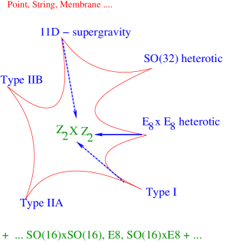
Figure 1: Perturbative treatment of elementary particles characterises them as idealised points, strings or membranes, … The non–perturbative dualities of supersymmetric string theories in ten dimensions, as well as 11 dimensional supergravity suggests probing the properties of different classes of string compactifications in the different limits. Uncovering the string dynamics will necessitate bringing the non–supersymmetric vacua into the fold as well.

that the different string theories are limits of a more fundamental theory. This is an important lesson because it shows that theories that look distinct from the point of view of the effective field theory limit, are in fact related in string theory by various duality transformations. Similarly, the observation of the spinor–vector duality tells us that the myriad of string vacua with different physical content in the effective field theory limit should not be taken at face value. The dynamical picture in string theory may be very different from what is indicated in the static limits. In this context, it is also vital to explore not only the stable supersymmetric configurations, but also non–stable configurations, compactified on the same underlying manifolds. As depicted in figure 1, different limits should be compactified on the same underlying manifold, being $Z_{2}\times Z_{2}$ orbifold in this case study, as well as the non–supersymmetric and tachyonic vacua, to explore the similarities and distinctions in the different cases. It should be anticipated that non of the perturbative limits can fully characterise the real vacuum. At best the perturbative limits can provide effective probes that can capture some of its properties. For example, the embedding of the Standard Model states in spinorial 16 representations of $SO(10)$ can only be gleaned in the heterotic $E_{8}\times E_{8}$ string, because it is the only limit that gives rise to spinorial representations in its perturbative spectrum. On the other hand, the dilaton has a run away behaviour in this limit and stabilising the dilaton necessitates moving away from the perturbative $E_{8}\times E_{8}$ heterotic–string limit.

The $Z_{2}\times Z_{2}$ orbifold compactifications have been most extensively studied in the free fermionic formulation of the heterotic-string in four dimensions. This formulation is equivalent to the toroidal orbifold construction. For any free fermion model one can find the bosonic equivalent z2xz2 , and the two representations have their respective merits. In particular, in the fermionic formulation many discrete torsions that are a priori turned off in the orbifold constructions, appear as free phases in the free fermionic models. This is particularly noted in the case of the spinor–vector duality, which is induced by discrete torsion between the orbifold $Z_{2}$ twist and the $Z_{2}$ Wilson line that breaks $E_{8}\times E_{8}\rightarrow SO(16)\times SO(16)$. On the other hand, in the orbifold construction there is a clear separation between the internal and Wilson line moduli, which is blurred in the fermionic models. The free fermion formalism provides a robust framework to construct phenomenological string models and study their properties.

In the fermionic formulation of the heterotic–string in four dimensions all the worldsheet degrees of freedom needed to cancel the conformal anomaly are represented in terms of two dimensional free fermions on the string worldsheet. The 64 worldsheet fermions the lightcone gauge are denoted as:

   ${\underline{{\hbox{Left-Movers}}}}$:                             $\psi^{\mu},~{}~{}{\chi_{i}},~{}~{}{y_{i},~{}~{}\omega_{i}}~{}~{}~{}~{}(\mu=1,2,~{}i=1,\cdots,6)$

   ${\underline{{\hbox{Right-Movers}}}}$

$${\bar{\phi}}_{A=1,\cdots,44}=\begin{cases}~{}~{}{{\bar{y}}_{i}~{},~{}{\bar{\omega}}_{i}}&i=1,{\cdots},6\cr&\cr~{}~{}{{\bar{\eta}}_{i}}&i=1,2,3{}{}\cr~{}~{}{{\bar{\psi}}_{1,\cdots,5}}&\cr~{}~{}{{\bar{\phi}}_{1,\cdots,8}}&\end{cases}$$

Where $\{y,\omega|{\bar{y}},{\bar{\omega}}\}^{1,\cdots,6}$ correspond to the internal manifold six compactified dimensions; ${\bar{\psi}}^{1,\cdots,5}$ produce the $SO(10)$ GUT symmetry; ${\bar{\phi}}^{1,\cdots,8}$ generate the hidden sector gauge symmetry; and ${\bar{\eta}}^{1,2,3}$ produce three $U(1)$ symmetries in the observable sector. Models in the free fermionic formulation are written in terms of a set of boundary condition basis vectors, which denote the transformation properties of the fermions around the noncontractible loops of the vacuum to vacuum amplitude, and the Generalised GSO (GGSO) projection coefficients of the one loop partition function fff .

3 Classification of fermionic $Z_{2}\times Z_{2}$ orbifolds

The early free fermionic models consisted of isolated examples with a shared underlying GUT structure fsu5 ; fny ; so64 ; lrs . The basis vectors spanning the different cases contained the NAHE–set vectors nahe , denoted as $\{{\bf 1},S,b_{1},b_{2},b_{3}\}$. The NAHE–set gives rise to an $SO(10)\times SO(6)^{3}\times E_{8}$ gauge symmetry, with forty–eight multiplets in the spinorial 16 representation of $SO(10)$, arising from the three twisted sectors of the $Z_{2}\times Z_{2}$ orbifold $b_{1}$, $b_{2}$ and $b_{3}$. The $S$–vector generates $N=4$ spacetime supersymmetry, which is reduced to $N=2$ by the basis vector $b_{1}$ and to $N=1$ by the inclusion of both $b_{1}$ and $b_{2}$. The NAHE–set is augmented with three or four additional basis vectors, typically denoted as $\{\alpha,\beta,\gamma\}$, which break the $SO(10)$ gauge symmetry to one of its subgroups. and simultaneously reduce the number of generations to three. In the standard–like models fny the $SO(10)$ gauge symmetry is broken to $SU(3)\times SU(2)\times U(1)_{B-L}\times U(1)_{R}$, and the weak hypercharge is given by the combination

$$U(1)_{Y}=T_{3_{R}}+{1\over 2}(B-L)\in SO(10).$$

Each of the $b_{1}$, $b_{2}$ and $b_{3}$ sectors produces one generation that form complete 16 multiplets of $SO(10)$. The models admit the needed scalar states to further reduce the gauge symmetry and to produce a viable fermion mass and mixing spectrum tqmp ; fermionmasses ; nmasses .

Since 2003, systematic classification of $Z_{2}\times Z_{2}$ heterotic–string orbifolds have been developed using the free fermionic model building rules. The classification method was initially developed for the spinorial 16 and $\overline{\bf 16}$ representations in vacua with unbroken $SO(10)$ gauge group so10class , and subsequently extended to include vectorial 10 representations so10c10 . This led to the discovery of Spinor–Vector Duality (SVD) in the space of fermionic $Z_{2}\times Z_{2}$ orbifold compactification, where the duality transformation is induced by exchange of GGSO phases. The classification method was subsequently extended to vacua with: $SO(6)\times SO(4)$ so64class ; $SU(5)\times U(1)$ fsu5class ; $SU(3)\times SU(2)\times U(1)^{2}$ slmclass ; $SU(3)\times U(1)\times SU(2)^{2}$ lrsranclass ; lrsferclass , unbroken subgroups of $SO(10)$. In this classification method the string models are generated by a fixed set of boundary condition basis vectors, consisting of twelve to fourteen basis vectors, $B=\{v_{1},v_{2},\dots,v_{14}\}.$ The models with unbroken $SO(10)$ group are produced by a set of twelve basis vectors

$$v_{1}={\bf 1} = \{\psi^{\mu},\ \chi^{1,\dots,6},y^{1,\dots,6},\omega^{1,\dots,6}~{}~{}~{}|~{}~{}~{}\bar{y}^{1,\dots,6},\bar{\omega}^{1,\dots,6},\bar{\eta}^{1,2,3},\bar{\psi}^{1,\dots,5},\bar{\phi}^{1,\dots,8}\},$$

$$v_{2}=S = \{\psi^{\mu},\chi^{1,\dots,6}\},$$

$$v_{3}=z_{1} = \{\bar{\phi}^{1,\dots,4}\},$$

$$v_{4}=z_{2} = \{\bar{\phi}^{5,\dots,8}\},$$ (3.1)

$$v_{4+i}=e_{i} = \{y^{i},\omega^{i}|\bar{y}^{i},\bar{\omega}^{i}\},\ i=1,\dots,6,~{}~{}~{}~{}~{}~{}~{}~{}~{}~{}~{}~{}~{}~{}~{}~{}~{}~{}~{}~{}~{}N=4~{}~{}{\rm Vacua}$$

$$v_{11}=b_{1} = \{\chi^{34},\chi^{56},y^{34},y^{56}|\bar{y}^{34},\bar{y}^{56},\bar{\eta}^{1},\bar{\psi}^{1,\dots,5}\},~{}~{}~{}~{}~{}~{}~{}~{}N=4\rightarrow N=2$$

$$v_{12}=b_{2} = \{\chi^{12},\chi^{56},y^{12},y^{56}|\bar{y}^{12},\bar{y}^{56},\bar{\eta}^{2},\bar{\psi}^{1,\dots,5}\},~{}~{}~{}~{}~{}~{}~{}~{}N=2\rightarrow N=1.$$

The first ten basis vectors preserve $N=4$ spacetime supersymmetry. The vectors $b_{1}$ and $b_{2}$ are $Z_{2}\times Z_{2}$ orbifold twists, and the third twisted sector is obtained as the combination $b_{3}=b_{1}+b_{2}+x$, where the $x$–sector is given by the combination

$$x={\bf 1}+S+\sum_{i=1}^{6}e_{i}+\sum_{k=1}^{2}z_{k}=\{{\bar{\psi}}^{1,\cdots,5},{\bar{\eta}}^{1,2,3}\}.$$ (3.2)

The breaking pattern $SO(10)\rightarrow SO(6)\times SO(4)$ is obtained by including in the basis the vector so64class

$$v_{13}=\alpha=\{\bar{\psi}^{4,5},\bar{\phi}^{1,2}\},$$ (3.3)

whereas $SO(10)\rightarrow SU(5)\times U(1)$ is achieved with the basis vector fsu5class

$$v_{13}=\alpha=\{\overline{\psi}^{1,\dots,5}=\textstyle\frac{1}{2},\overline{\eta}^{1,2,3}=\textstyle\frac{1}{2},\overline{\phi}^{1,2}=\textstyle\frac{1}{2},\overline{\phi}^{3,4}=\textstyle\frac{1}{2},\overline{\phi}^{5}=1,\overline{\phi}^{6,7}=0,\overline{\phi}^{8}=0\,\},$$ (3.4)

and $SO(10)\rightarrow SU(3)\times SU(2)\times U(1)^{2}$ is obtained by adding (3.3) and (3.4) as two separate vectors, $v_{13}$ and $v_{14}$ to the basis slmclass . The breaking of the $SO(10)$ gauge symmetry to the Left–Right Symmetric (LRS) subgroup is obtained with the basis vector lrsranclass ,

$$v_{13}=\alpha=\{\overline{\psi}^{1,2,3}=\frac{1}{2}\;,\;\overline{\eta}^{1,2,3}=\frac{1}{2}\;,\;\overline{\phi}^{1,\ldots,6}=\frac{1}{2}\;,\;\overline{\phi}^{7}\}.$$ (3.5)

For a fixed set of basis vectors, the space of models is spanned by varying the independent GGSO projection coefficients. For example, in the $SO(6)\times SO(4)$ models 66 phases are taken to be independent

$$\bordermatrix{&1&S&e_{1}&e_{2}&e_{3}&e_{4}&e_{5}&e_{6}&z_{1}&z_{2}&b_{1}&b_{2}&\alpha\cr 1&-1&-1&\pm&\pm&\pm&\pm&\pm&\pm&\pm&\pm&\pm&\pm&\pm\cr S~{}&&&-1&-1&-1&-1&-1&-1&-1&-1&1&1&-1\cr e_{1}~{}&&&&\pm&\pm&\pm&\pm&\pm&\pm&\pm&\pm&\pm&\pm\cr e_{2}~{}&&&&&\pm&\pm&\pm&\pm&\pm&\pm&\pm&\pm&\pm\cr e_{3}~{}&&&&&&\pm&\pm&\pm&\pm&\pm&\pm&\pm&\pm\cr e_{4}~{}&&&&&&&\pm&\pm&\pm&\pm&\pm&\pm&\pm\cr e_{5}~{}&&&&&&&&\pm&\pm&\pm&\pm&\pm&\pm\cr e_{6}~{}&&&&&&&&&\pm&\pm&\pm&\pm&\pm\cr z_{1}~{}&&&&&&&&&&\pm&\pm&\pm&\pm\cr z_{2}~{}&&&&&&&&&&&\pm&\pm&\pm\cr b_{1}~{}&&&&&&&&&&&&\pm&\pm\cr b_{2}~{}&&&&&&&&&&&&&\pm\cr\alpha~{}&&&&&&&&&&&&&\cr},$$

where the diagonal terms and below are fixed by modular invariance constraints. The remaining fixed phases are set by requiring $N=1$ spacetime supersymmetry and the overall chirality. Varying the 66 independent phases randomly scans a space of $2^{66}$ (approximately $10^{19.9}$) $Z_{2}\times Z_{2}$ heterotic–string orbifold models. A specific choice of the 66, $\pm 1$ phases corresponds to a distinct string vacuum with massless and massive physical spectrum. The analysis proceeds by developing systematic tools to analyse the entire massless spectrum, as well as the leading top quark Yukawa coupling topyukawa . Random choices of the 66 GGSO phases, are generated and the spectrum is extracted systematically. A suitable algorithm has to be implemented to ensure that identical models are not generated. This is typically assisted by requiring that the random cycle is sufficiently long and that the probability for the generation of identical sequences is very small. It should be noted though that the utility of the random generation method reaches its limit when the space becomes to large slmclass ; towardmac . Genetic algorithm provides a more efficient trawling tool to fish out models with specific characteristics abelrizos . On the other hand, genetic algorithms are not suited to classifying and sorting large spaces of vacua. A more suitable approach for that purpose is offered by application of Satisfiability Modulo Theories, that can reduce the computer run time by three orders of magnitude fpsw .

4 Spinor–vector duality in heterotic–string orbifolds

The free fermionic classification methodology led to the discovery of spinor–Vector Duality (SVD), depicted in figure 2, under the exchange of the total number of $({\bf 16}+\overline{\bf 16})$ spinorial and 10 vectorial representations of $SO(10)$ so10c10 . The SVD arises from the breaking $(2,2)~{}\rightarrow~{}(2,0)$ worldsheet supersymmetry. It is a general property of heterotic–string vacua. From a worldsheet perspective, the SVD suggests that all string vacua are connected by interpolations or by orbifolds, but are distinct in the low energy effective field theory spwsp .

Figure 2: Density plot showing the spinor–vector duality in the space of fermionic $Z_{2}\times Z_{2}$ heterotic–string models. The plot shows the number of vacua with a given number of $({\bf 16}+\overline{\bf 16})$ and 10 multiplets of $SO(10)$. It is invariant under exchange of rows and columns, reflecting the spinor–vector duality underlying the entire space of vacua. Models on the diagonal are self–dual under the exchange of rows and columns, i.e. $\#({\bf 16}+\overline{16})=\#({\bf 10})$ without enhancement to $E_{6}$, which are self–dual by virtue of the enhanced symmetry.

Further insight into the spinor-vector duality is obtained by translating to the bosonic $Z_{2}\times Z_{2}$ representation. First, it is noted that in the fermionic constructions the SVD operates separately in each of the $Z_{2}$ planes, which preserve $N=2$ spacetime supersymmetry. Hence, we can study the SVD in vacua with a single $Z_{2}$ twist of the compactified coordinates fkrneq2 . Using the level one $SO(2n)$ characters

$$O_{2n}={1\over 2}\left({\theta_{3}^{n}\over\eta^{n}}+{\theta_{4}^{n}\over\eta^{n}}\right)\,,~{}~{}~{}~{}~{}~{}~{}~{}~{}~{}~{}~{}V_{2n}={1\over 2}\left({\theta_{3}^{n}\over\eta^{n}}-{\theta_{4}^{n}\over\eta^{n}}\right)\,,~{}~{}~{}~{}~{}~{}~{}~{}~{}~{}~{}~{}S_{2n}={1\over 2}\left({\theta_{2}^{n}\over\eta^{n}}+i^{-n}{\theta_{1}^{n}\over\eta^{n}}\right)\,,~{}~{}~{}~{}~{}~{}~{}C_{2n}={1\over 2}\left({\theta_{2}^{n}\over\eta^{n}}-i^{-n}{\theta_{1}^{n}\over\eta^{n}}\right)\,,$$ (4.1)

where

$${\theta_{3}\equiv Z_{f}{0\choose 0}~{}~{}~{}\theta_{4}\equiv Z_{f}{0\choose 1}~{}~{}~{}}{\theta_{2}\equiv Z_{f}{1\choose 0}~{}~{}~{}\theta_{1}\equiv Z_{f}{1\choose 1}~{},~{}~{}}$$

and $Z_{f}$ is the partition function of a single worldsheet complex fermion, given in terms of theta functions manno , the partition function of the heterotic $E_{8}\times E_{8}$ string compactified to four dimensions

$${Z}_{+}=(V_{8}-S_{8})\,\left(\sum_{m,n}\Lambda_{m,n}\right)^{\otimes 6}\,\left(\overline{O}_{16}+\overline{S}_{16}\right)\left(\overline{O}_{16}+\overline{S}_{16}\right)\,,$$ (4.2)

where as usual, for each circle,

$$p_{\rm L,R}^{i}={m_{i}\over R_{i}}\pm{n_{i}R_{i}\over\alpha^{\prime}}\,~{}~{}~{}~{}~{}~{}~{}~{}~{}{\rm and}~{}~{}~{}~{}~{}~{}~{}~{}~{}\Lambda_{m,n}={q^{{\alpha^{\prime}\over 4}p_{\rm L}^{2}}\,\bar{q}^{{\alpha^{\prime}\over 4}p_{\rm R}^{2}}\over|\eta|^{2}}\,.$$

A $Z_{2}\times Z_{2}^{\prime}:g\times g^{\prime}$ action is applied. The first $Z_{2}$ is freely acting. It couples a fermion number in the observable and hidden sectors with a $Z_{2}$–shift in a compactified coordinate, and is given by $g:(-1)^{(F_{1}+F_{2})}\delta$  where the fermion numbers $F_{1,2}$ act on the spinorial representations of the observable and hidden $SO(16)$ groups as $F_{1,2}:({\overline{O}}_{16}^{1,2},{\overline{V}}_{16}^{1,2},{\overline{S}}_{16}^{1,2},{\overline{C}}_{16}^{1,2})\longrightarrow~{}({\overline{O}}_{16}^{1,2},{\overline{V}}_{16}^{1,2},-{\overline{S}}_{16}^{1,2},-{\overline{C}}_{16}^{1,2})$  and $\delta$ identifies points shifted by a $Z_{2}$ shift in the $X_{9}$ direction, i.e. $\delta X_{9}=X_{9}+\pi R_{9}.~{}$ The effect of the shift is to insert a factor of $(-1)^{m}$ into the lattice sum in eq. (4.2), i.e. $\delta:\Lambda_{m,n}^{9}\longrightarrow(-1)^{m}\Lambda_{m,n}^{9}.$  The second $Z_{2}$ acts as a twist on the internal coordinates given by ${g^{\prime}}:(x_{4},x_{5},x_{6},x_{7},x_{8},x_{9})\longrightarrow(-x_{4},-x_{5},-x_{6},-x_{7},+x_{8},+x_{9}).$ Alternatively, the first $Z_{2}$ action can be interpreted as a Wilson line in $X_{9}$ ffmt , $g~{}:(0^{7},1|1,0^{7})~{}\rightarrow~{}E_{8}\times E_{8}\rightarrow SO(16)\times SO(16).$ The effect of the single space twisting is to break $N=4\rightarrow N=2$ spacetime supersymmetry and $E_{8}\rightarrow E_{7}\times SU(2)$ or with the inclusion of the Wilson line $SO(16)\rightarrow SO(12)\times SO(4)$. The orbifold partition function is given by

$${Z~{}=~{}\left({Z_{+}\over{Z_{g}\times Z_{g^{\prime}}}}\right)~{}=~{}\left[{{(1+g)}\over 2}{{(1+g^{\prime})}\over 2}\right]~{}Z_{+}}.$$

The partition function contains an untwisted sector and three twisted sectors. It has the schematic form shown in figure 3. The winding modes in the sectors twisted by $g$ and $gg^{\prime}$ are shifted by $1/2$, and therefore these sectors only produce massive states. The sector twisted by $g$ gives rise to the massless twisted matter states. The partition function has two modular orbits and one discrete torsion $\epsilon=\pm 1$. Massless states are obtained for vanishing lattice modes. The terms in the sector $g$ contributing to the massless spectrum take the form

$$\Lambda_{p,q}\left\{{1\over 2}\left(\left|{{2\eta}\over\theta_{4}}\right|^{4}+\left|{{2\eta}\over\theta_{3}}\right|^{4}\right)\left[{P_{\epsilon}^{+}Q_{s}{\overline{V}}_{12}{\overline{C}}_{4}{\overline{O}}_{16}}+{P_{\epsilon}^{-}Q_{s}{\overline{S}}_{12}{\overline{O}}_{4}{\overline{O}}_{16}}\right.{\left.\right]+}\right.$$

$$\left.~{}~{}~{}~{}~{}~{}~{}~{}~{}~{}{1\over 2}\left(\left|{{2\eta}\over\theta_{4}}\right|^{4}-\left|{{2\eta}\over\theta_{3}}\right|^{4}\right)\left[{P_{\epsilon}^{+}Q_{s}{\overline{O}}_{12}{\overline{S}}_{4}{\overline{O}}_{16}}\right.{\left.\right]}\right\}~{}~{}~{}~{}~{}~{}~{}~{}~{}~{}~{}~{}~{}~{}~{}~{}~{}~{}~{}~{}~{}~{}~{}~{}~{}~{}~{}~{}+~{}~{}\hbox{massive}$$ (4.3)

where

$$P_{\epsilon}^{+}~{}=~{}\left({{1+\epsilon(-1)^{m}}\over 2}\right)\Lambda_{m,n}~{}~{}~{};~{}~{}~{}P_{\epsilon}^{-}=\left({{1-\epsilon(-1)^{m}}\over 2}\right)\Lambda_{m,n}$$ (4.4)

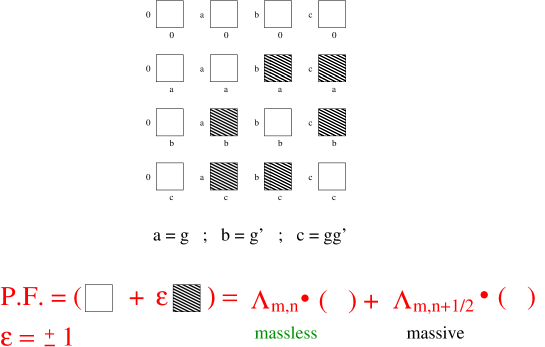
Figure 3: The $Z_{2}\times Z_{2}^{\prime}$ partition function of the $g$–twist and $g^{\prime}$ Wilson line with discrete torsion $\epsilon=\pm 1$.

Depending on the sign of $\epsilon=\pm$ it is seen from eq. (4.4) that either the vectorial states, or the spinorial states, are massless. In the case with $\epsilon=+1$ we note from eq. (4.5) that in this case massless momentum modes from the shifted lattice arise in $P_{\epsilon}^{+}$ whereas $P_{\epsilon}^{-}$ only produces massive modes. Therefore, in his case the vectorial character ${\overline{V}}_{12}$ in eq. (4.4) produces massless states, whereas the spinorial character ${\overline{S}}_{12}$ generates massive states. In the case with $\epsilon=-1$ eq. (4.6) shows that exactly the opposite occurs.

$${\epsilon~{}=~{}+1~{}~{}} {\Rightarrow} {~{}~{}P^{+}_{\epsilon}~{}=~{}~{}~{}~{}~{}~{}~{}~{}~{}~{}~{}\Lambda_{2m,n}~{}~{}~{}~{}~{}~{}~{}~{}~{}~{}~{}~{}~{}~{}~{}{P^{-}_{\epsilon}~{}=~{}~{}~{}~{}~{}~{}~{}~{}\Lambda_{2m+1,n}}~{}~{}~{}}$$ (4.5)

$${\epsilon~{}=~{}-1~{}~{}} {\Rightarrow} {{~{}~{}P^{+}_{\epsilon}~{}=~{}~{}~{}~{}~{}~{}~{}~{}~{}~{}~{}\Lambda_{2m+1,n}}~{}~{}~{}~{}~{}~{}~{}~{}~{}~{}~{}~{}P^{-}_{\epsilon}~{}=~{}~{}~{}~{}~{}~{}~{}~{}\Lambda_{2m,n}~{}~{}~{}}$$ (4.6)

Thus, the spinor–vector duality is generated by the exchange of the discrete torsion $\epsilon=+1\rightarrow\epsilon=-1$ in the $Z_{2}\times Z_{2}^{\prime}$ partition function. This is very similar the the case of mirror symmetry in the $Z_{2}\times Z_{2}$ orbifold model of ref. vafawitten , where the mirror symmetry map is induced by exchange of the discrete torsion between the two orbifold $Z_{2}$ twists. In the mirror symmetry case the chirality of the fermion multiplets is changed, together with the exchange of the complex and Kähler moduli of the internal manifold. The total number of degrees of freedom is invariant under the mirror symmetry map. It is interesting to note that this is also the case in the case of the SVD. In this case there is a mismatch between the number of states in the vectorial, $12\cdot 2=24$, and spinorial $32$, cases. It is noted from the second line in eq. (4.3) that the vectorial case $\epsilon=+1$ is accompanied by $8$ additional states, which are singlets of the $SO(12)$ GUT group. It is seen that the total number of degrees of freedom is preserved under the duality map, i.e. ${12\cdot 2+4\cdot 2}{=}{32}.$

What can be inferred from the spinor–vector duality? What lessons can we draw from the example of mirror symmetry, which was initially observed in worldsheet string constructions? Mirror symmetry has profound implications for the geometry of the internal manifold in the effective field theory limit of the string compactifications. The SVD tells us that vacua that look distinct from the point view of the effective field theory limit are in fact connected in the worldsheet description, because in the string construction massless and massive mode can be exchanged. Furthermore, the matching of the massless degrees of freedom in the different cases tells us that the worldsheet string theory primarily cares about obtaining the number of degrees of freedom required in a modular invariant partition function, whereas how they are organised in representations of the four dimensional gauge symmetry is of secondary importance. It is of further interest to explore the implications of the SVD in the effective field theory limit of the string compactifications. The SVD can serve as a probe of the moduli spaces of heterotic–string compactifications with $(2,0)$ worldsheet supersymmetry. While the moduli spaces of string compactifications with standard embedding and $(2,2)$ worldsheet supersymmetry are fairly well understood, the case of $(2,0)$ models is obscured. The SVD can provide a very useful probe of these models that in the string picture can be seen as deformations of the $(2,2)$ cases, whereas in the effective QFT picture they correspond to compactifications on Calabi-Yau manifolds with vector bundles. Recently, we demonstrated the viability of these approach in the case of compactifications to six and five dimensions fgh , where the effective field theory limit is obtained by resolving the orbifold singularities. In this context, the worldsheet description serves as a guide to guess how the discrete torsion of the worldsheet description should be interpreted in the effective field theory limit. In this respect, it is noted that the SVD in the worldsheet formalism generalises to string compactifications with interacting internal CFTs afg , as well as to cases that include more discrete torsions aft .

5 Low scale $Z^{\prime}$ in free fermionic models

The interest in extra $Z^{\prime}$ vector bosons at low scales in string derived models stems from the role that the $U(1)$ symmetry can play in explaining some of the features of the Standard Model or the supersymmetric Standard Model. This include suppression of proton decay mediating operators and of the $\mu$–term in supersymmetric models. However, construction of string models that allow an extra $U(1)$ symmetry to remain unbroken down to intermediate or low scales has proven to be non–trivial. The first case to be considered so10zprime was the combination

$$U(1)_{Z^{\prime}}={3\over 2}U(1)_{B-L}-2U(1)_{R}\in SO(10),$$ (5.1)

which ensures suppression of proton decay from dimension four operators. However, the underlying $SO(10)$ symmetry in the string models implies that the Dirac mass terms of the tau neutrino and top quark are equal, necessitating the breaking of (5.1) at high scale tauneutrino . A more natural possibility is that this $U(1)_{Z^{\prime}}$ symmetry is broken at a high scale, which generates a large scale seesaw and naturally produces light neutrino masses nmasses . Existence of alternative $U(1)$ symmetries in the string models that suppress the proton decay mediating operators and allow a high seesaw mass scale were discussed in none6zprime . However, those tend to fail as low scale candidates, because they are either non–family universal or have to be broken by the supersymmetric $F$– and $D$–flatness constraints. Furthermore, the additional family universal $U(1)\in E_{6}$ is generically anomalous in the string models because of the symmetry breaking pattern $E_{6}\rightarrow SO(10)\times U(1)$ that projects out some of components of the chiral $27$ and $\overline{27}$ representations of $E_{6}$ u1a . On the other hand, gauge coupling unification favours extra low scale $U(1)$ with an $E_{6}$ embedding of its matter states viraf .

The construction of string models that allow an extra $U(1)\in E_{6}$ to remain unbroken down to low scale can follow one of two routes. The first is to use a different symmetry breaking pattern than the $E_{6}\rightarrow SO(10)\times U(1)$ route. This symmetry breaking pattern follows from the underlying breaking of $E_{8}\times E_{8}\rightarrow SO(16)\times SO(16)$, which is commonly used in the free fermion models. A different route would essentially correspond to keeping in the spectrum the spacetime vector bosons from the $x$–sector, which enhances $SO(16)\rightarrow E_{8}$. An example of a string derived model in this class is the $SU(6)\times SU(2)$ model of ref. e8patterns .

An alternative route, pursued in ref. frzprime , is to use the spinor–vector duality. As discussed above, in string models with $E_{6}$ symmetry, the $U(1)_{A}\in SO(10)\times U(1)$ combination is family universal by virtue of its embedding in $E_{6}$. The $E_{6}$ representations are self–dual under the spinor–vector duality and $U(1)_{A}$ is anomaly free. However, we can obtain models which are self–dual under SVD without enhancement of the $SO(10)\times U(1)$ gauge symmetry to $E_{6}$. In this case the twisted matter representations still form complete $E_{6}$ multiplets, which results in the universal $U(1)\in E_{6}$ combination being anomaly free, without, however, enhancement of the gauge symmetry to $E_{6}$. A set of phases producing a model with the required properties is shown in eq. (5.2). The observable gauge group in the model is $SO(6)\times SO(4)\times U(1)_{1,2,3}$ and the family universal combination, $U(1)_{\zeta}=U(1)_{1}+U(1)_{2}+U(1)_{3}$, is anomaly free.

$$(v_{i}|v_{j})\ \ =\ \ \bordermatrix{&1&S&e_{1}&e_{2}&e_{3}&e_{4}&e_{5}&e_{6}&b_{1}&b_{2}&z_{1}&z_{2}&\alpha\cr 1&1&1&1&1&1&1&1&1&1&1&1&1&1\cr S&1&1&1&1&1&1&1&1&1&1&1&1&1\cr e_{1}&1&1&0&0&0&0&0&0&0&0&0&0&1\cr e_{2}&1&1&0&0&0&0&0&1&0&0&0&1&0\cr e_{3}&1&1&0&0&0&1&0&0&0&0&0&1&1\cr e_{4}&1&1&0&0&1&0&0&0&0&0&1&0&0\cr e_{5}&1&1&0&0&0&0&0&1&0&0&0&1&1\cr e_{6}&1&1&0&1&0&0&1&0&0&0&1&0&0\cr b_{1}&1&0&0&0&0&0&0&0&1&1&0&0&0\cr b_{2}&1&0&0&0&0&0&0&0&1&1&0&0&1\cr z_{1}&1&1&0&0&0&1&0&1&0&0&1&1&0\cr z_{2}&1&1&0&1&1&0&1&0&0&0&1&1&0\cr\alpha&1&1&1&0&1&0&1&0&1&0&1&0&1\cr}$$ (5.2)

The complete massless spectrum, as well as the tri–level superpotential are given in ref. frzprime . The massless chiral spectrum in the model is self–dual under the spinor–vector duality. The model contains three chiral generations, as well as the required heavy and light Higgs states to produce a realistic fermion mass spectrum, as well as a cubic level top quark Yukawa coupling. A VEV of the heavy Higgs field that breaks the Pati–Salam symmetry to the Standard Model along flat directions leaves the unbroken combination

$$U(1)_{Z^{\prime}}~{}~{}=~{}~{}{1\over 5}~{}U(1)_{C}~{}~{}-~{}~{}{1\over 5}~{}U(1)_{L}-U_{\zeta}.$$ (5.3)

This $U(1)$ symmetry is anomaly free in this model and may remain unbroken down to low scales.

6 String inspired BSM phenomenology

The string derived model gives rise to an extra $U(1)_{Z^{\prime}}$ combination given in eq. (5.3). There are numerous reasons that motivate the possibility that this $U(1)$ symmetry remains unbroken down to low scales. To explore the phenomenological implications of the model we can choose the low scale spectrum to be consistent with the existence of the $U(1)$ symmetry at low scales and impose some additional conditions inspired from the string derived model. For example, we can fix the top quark Yukawa coupling to be given by $\lambda_{t}=\sqrt{2}g$, where $g$ is the gauge coupling at the heterotic–string unification scale tqmp . Similarly, the Yukawa couplings of the lighter quarks and leptons can be calculated in the model from higher order non–renormalisable operators fermionmasses and detailed mass textures can be obtained. Naturally, more details are subject to increasing model dependence and requires making further assumptions, e.g. assumptions on a SUSY breaking mechanism and SUSY breaking parameters. At this stage the analysis is inspired from the string derived model and uses some input parameters fixed by the string model. In this spirit, we can fix the spectrum of the string inspired model, as given in table 6.

Spectrum and $SU(3)_{C}\times SU(2)_{L}\times U(1)_{Y}\times U(1)_{{Z}^{\prime}}$ quantum numbers, with $i=1,2,3$ for the three light generations. The charges are displayed in the normalisation used in free fermionic heterotic–string models. Field $\hphantom{\times}SU(3)_{C}$ $\times SU(2)_{L}$ ${U(1)}_{Y}$ ${U(1)}_{Z^{\prime}}$ $Q_{L}^{i}$ $3$ $2$ $+\frac{1}{6}$ $-\frac{2}{5}$ $u_{L}^{i}$ ${\bar{3}}$ $1$ $-\frac{2}{3}$ $-\frac{2}{5}$ $d_{L}^{i}$ ${\bar{3}}$ $1$ $+\frac{1}{3}$ $-\frac{4}{5}$ $e_{L}^{i}$ $1$ $1$ $+1$ $-\frac{2}{5}$ $L_{L}^{i}$ $1$ $2$ $-\frac{1}{2}$ $-\frac{4}{5}$ $D^{i}$ $3$ $1$ $-\frac{1}{3}$ $+\frac{4}{5}$ ${\bar{D}}^{i}$ ${\bar{3}}$ $1$ $+\frac{1}{3}$ $+\frac{6}{5}$ $H^{i}$ $1$ $2$ $-\frac{1}{2}$ $+\frac{6}{5}$ ${\bar{H}}^{i}$ $1$ $2$ $+\frac{1}{2}$ $+\frac{4}{5}$ $S^{i}$ $1$ $1$   $0$ $-2$ $h$ $1$ $2$ $-\frac{1}{2}$ $-\frac{4}{5}$ ${\bar{h}}$ $1$ $2$ $+\frac{1}{2}$ $+\frac{4}{5}$ $\phi$ $1$ $1$   $0$ $-1$ $\bar{\phi}$ $1$ $1$   $0$ $+1$ $\zeta^{i}$ $1$ $1$   $0$   $0$

It is noted that anomaly cancellation of the extra $U(1)_{Z^{\prime}}$ symmetry requires the existence of additional matter states at the $Z^{\prime}$ breaking scale. These additional matter states may have profound implications on experimental searches beyond the Standard Model, and may in fact be associated with the recent observed deviations from the expected Standard Model values in lepton universality LHCbExp and muon $g-2$ gminus2 experiments. A quick glance in table (6) makes this evident. The model predicts the existence of additional $SU(2)$ doublets and $SU(3)$ triplets that are chiral under the extra $U(1)_{Z^{\prime}}$ but are vector–like with respect to the Standard Model gauge group. The natural mass scale for these states is the $U(1)_{Z^{\prime}}$ breaking scale. On the other hand, these additional electroweak doublets and colour triplets are precisely the type of states that may explain the deviations from the Standard Model predictions, via their contributions in multi–loop diagrams.

Additionally, the existence of the extra $SO(10)$ singlet fields $S_{i}$ in table 6 may explain the generation of the electroweak scale, via dimensional transmutation. As seen in table 6, gauge coupling unification at the heterotic–string scale suggests the existence of an additional pair of Higgs doublets, beyond those that are required by anomaly cancellation. This pair of additional doublets is somewhat ad hoc, but beyond that, the traditional mixing term between the chiral doublets is generated by the VEV of the $S_{i}$ fields. Thus, the low scale breaking of $U(1)_{Z^{\prime}}$ and the ensuing electroweak symmetry breaking can be nicely incorporated in the $Z^{\prime}$ model.

From table 6 it seen that the model predicts the existence of sterile neutrinos. Three sterile neutrinos are obtained from the Standard Model singlets in the spinorial 16 representation of $SO(10)$. Mass terms for these states are generated at the seesaw high mass scale, and they decouple from the effective low scale field theory at that scale. Additionally, the model contain the three $SO(10)$ singlet states $S_{i}$, which can appear as low scale sterile neutrinos nmasses . Existence of sterile neutrinos in this model is correlated with the existence of a low scale extra $U(1)_{Z^{\prime}}$ symmetry that protects the sterile neutrinos from acquiring high scale mass.

7 Spinor–vector duality and modular maps

Modular maps are ubiquitous in string theory. By modular maps here I mean maps that are induced by basis vectors with four periodic fermions in the left– or right–moving sector. An example of such a map is given by the $S$–vector in eq. (3.1). The $S$–vector is the supersymmetry generator in the string models and maps bosonic to fermionic sectors. The spinor–vector duality can similarly be seen to arise from such a modular map. Further insight is obtained by using the set of boundary condition basis vectors given in eq. (7.1):

$$v_{1}=1 = \{\psi^{\mu},\ \chi^{1,\dots,6},y^{1,\dots,6},\omega^{1,\dots,6}|$$

$$~{}~{}~{}\bar{y}^{1,\dots,6},\bar{\omega}^{1,\dots,6},\bar{\eta}^{1,2,3},\bar{\psi}^{1,\dots,5},\bar{\phi}^{1,\dots,8}\},$$

$$v_{2}=S = \{\psi^{\mu},\chi^{1,\dots,6}\},$$

$$v_{3}=z_{1} = \{\bar{\phi}^{1,\dots,4}\},$$

$$v_{4}=z_{2} = \{\bar{\phi}^{5,\dots,8}\},$$

$$v_{5}=z_{3} = \{\bar{\psi}^{1,\dots,4}\},$$

$$v_{6}=z_{0} = \{\bar{\eta}^{0,1,2,3}\},$$

$$v_{7}=b_{1} = \{\chi^{34},\chi^{56},y^{34},y^{56}|\bar{y}^{34},\bar{y}^{56},\bar{\eta}^{0},\bar{\eta}^{1}\},$$ (7.1)

The models generated by the basis (7.1) preserve $N=2$ space–time supersymmetry, as the single supersymmetry breaking vector $b_{1}$ is included the basis.

The novel feature in the basis of eq. (7.1) is that the spacetime vector bosons that are obtained in the untwisted Neveu–Schwarz sector generate an $SO(12)\times SO(8)^{4}$ gauge symmetry at the $N=4$ level, i.e. prior to the inclusion of the vector $b_{1}$. The lattice $SO(12)$ symmetry arises from the internal right–moving degrees of freedom, $\{{\bar{y}},{\bar{\omega}}\}^{1,\cdots,6}$, at the enhanced symmetry point, whereas each of the $SO(8)^{4}$ symmetries arise from the four sets of worldsheet fermions $\{{\bar{\psi}}^{1,\cdots,4}\};\{{\bar{\eta}}^{0,1,2,3}\};\{{\bar{\phi}}^{1,\cdots,4}\};\{{\bar{\phi}}^{1,\cdots,6}\}$. With the the basis given in eq. (7.1), the GUT $SO(10)$ in $N=1$ models, or $SO(12)$ in $N=2$ models, is generated from vectors bosons in the purely anti–holomorphic sectors

$$G=\{ z_{0},z_{1},z_{2},z_{3},$$ (7.2)

$$z_{0}+z_{1},z_{0}+z_{2},z_{0}+z_{3},z_{1}+z_{2},z_{1}+z_{3},z_{2}+z_{3}~{}~{}\}.$$

The resulting gauge symmetries depend on the choices of GGSO projection coefficients and have been classified in ref. fkrneq2 . They contain the two cases $SO(12)\times E_{8}\times E_{8}$ and $SO(12)\times SO(16)\times SO(16)$ that are distinguished by the choice of the phase

$$c{z_{0}\atopwithdelims[ ]z_{1}}=\pm 1.$$

The $SO(12)\times SO(16)\times SO(16)$ gauge symmetry is realised with the GGSO projection coefficients taken as

$$c{z_{0}\atopwithdelims[ ]z_{1}}=~{}~{}c{z_{0}\atopwithdelims[ ]z_{3}}=~{}~{}c{z_{1}\atopwithdelims[ ]z_{2}}=c{z_{0}\atopwithdelims[ ]z_{2}}=-c{z_{1}\atopwithdelims[ ]z_{3}}=-c{z_{2}\atopwithdelims[ ]z_{3}}=-1,$$ (7.3)

where the enhancing vector bosons are obtained from the sectors $z_{2}$ and $z_{3}$. As discussed above, the basis vector $b_{1}$ breaks $N=4$ spacetime supersymmetry to $N=2$, and reduces gauge symmetry arising from the $0$–sector to

$$\left[SO(8)\times SO(4)\right]_{\cal L}\times\left[SO(8)_{3}\times SO(4)\times SO(4)\right]_{O}\times\left[SO(8)_{1}\times SO(8)_{2}\right]_{H}.$$ (7.4)

For the choice given in eq. (7.3) the vector $b_{1}$ breaks the $\left[SO(16)\right]_{O}\rightarrow\left[SO(12)\times SO(4)\right]_{O}\equiv\left[SO(12)\times SU(2)_{0}\times SU(2)_{1}\right]_{O}$. The realisation of the spinor–vector duality in this model is now discussed. First, consider the choice of additional phases given by:

$$c{b_{1}\atopwithdelims[ ]1,z_{0}}=-c{b_{1}\atopwithdelims[ ]S,z_{1},z_{2},z_{3}}=-1~{}.$$ (7.5)

In this case the model contains 2 multiplets in the $(1,2_{L}+2_{R},12,1,2,1)$ and 2 in the $(8,2_{L}+2_{R},1,2,1,1)$ representations of $\left[SO(8)\times SO(4)\right]_{\cal L}\times\left[SO(12)\times SU(2)_{0}\times SU(2)_{1}\right]_{O}\times\left[SO(16)\right]_{H}$. the sectors giving rise to the vectorial 12 representation of $SO(12)$ are the sectors $b_{1}$ and $b_{1}+z_{3}$, where the sector $b_{1}$ produces the $(1,2,2)$ representation and the sectors $b_{1}+z_{3}$ produces the $(8_{{}_{S}},1,1)$ under the decomposition $\left[SO(12)\right]_{O}\rightarrow\left[SO(8)\times SO(4)\right]_{O}\equiv\left[SO(8)\times SU(2)\times SU(2)\right]_{O}$. All other states are projected out. Therefore, there are a total of eight multiplets in the vectorial representation of the observable $SO(12)$ in this model, which also transform as doublets of the observable $SU(2)_{1}$.

The second choice of GGSO phases is given by

$$c{b_{1}\atopwithdelims[ ]1,z_{0},z_{1}}=-c{b_{1}\atopwithdelims[ ]S,z_{2},z_{3}}=-1$$ (7.6)

This choice produces a model with 2 multiplets in the $(1,2_{L}+2_{R},32,1,1,1)$, and 2 in the $(1,2_{L}+2_{R},1,1,2,16)$, representations of $\left[SO(8)\times SO(4)\right]_{\cal L}\times\left[SO(12)\times SU(2)_{0}\times SU(2)_{1}\right]_{O}\times\left[SO(16)\right]_{H}$. In this case the the sectors giving rise to the spinorial 32 representation of $\left[SO(12)\right]_{O}$ are the sectors $b_{1}+z_{0}$ and $b_{1}+z_{3}+z_{0}$, where the sector $b_{1}+z_{0}$ produces the $(8_{{}_{V}},2,1)$ representation and the sectors $b_{1}+z_{3}+z_{0}$ produces the $(8_{{}_{C}},1,2)$ under the decomposition $\left[SO(12)\right]_{O}\rightarrow\left[SO(8)\times SO(4)\right]_{O}\equiv\left[SO(8)\times SU(2)\times SU(2)\right]_{O}$. The sectors producing the vectorial 16 representation of the $SO(16)_{H}$ gauge group are the sectors $b_{1}$ and $b_{1}+z_{2}$, where the sector $b_{1}$ gives rise to the $(8_{{}_{V}},1)$ representation and the sector $b_{1}+z_{2}$ gives rise to the $(1,8_{{}_{C}})$ representation under the decomposition $\left[SO(16)\right]_{H}\rightarrow\left[SO(8)_{1}\times SO(8)_{2}\right]_{H}$. The hidden 16 representations transform as doublets of the observable $SU(2)_{1}$ group. All other states are projected out. There are a total of eight multiplets in the spinorial 32 representation of the observable $\left[SO(12)\right]_{O}$ in this model. The transformation between the two models, (7.5) and (7.6), is induced by the discrete GGSO phase change

$$c{b_{1}\atopwithdelims[ ]z_{1}}=+1~{}~{}\rightarrow~{}~{}c{b_{1}\atopwithdelims[ ]z_{1}}=-1$$ (7.7)

What is crucial, however, is the role played by the basis vector $z_{0}$ in eq. (7.1). This basis vector induces a map between the sectors that produce the spinorial states to those that produce vectorial states. Its role in this respect is similar to that performed by the $x$–vector in the basis of eq. (3.1), which induces the co–called $x$–map of refs. fermionmasses ; so10c10 ; cfkr . The $z_{0}$ basis vector is the analogue of the $S$ basis vector on the supersymmetric side of the heterotic–string. In the case of $N=1$ models with enhanced $E_{6}$ symmetry, it acts as a spectral flow operator that mixes the different components of the $E_{6}$ representations. In the models in which $E_{6}$ is broken to $SO(10)\times U(1)$, it induces the map between the spinor–vector dual models ffmt . The $z_{0}$ action is a second example of what is called here a “modular map”.

The two examples, the $S$–map and the $z_{0}$ map, are mere two examples of a much richer symmetry structure. This much richer symmetry structure is a topic of much interest in symmetries that underlie 24 dimensional lattices. What role this symmetry structure plays in the phenomenological properties of string theory is yet to be unravelled. The two examples above clearly demonstrate its potential, the first being SUSY phenomenology, whereas the second was investigated in the context of low scale $Z^{\prime}$ phenomenology. An embryonic attempt to link this rich symmetry structure to the phenomenological free fermionic constructions was discussed in ref. panosleech . In the next section, I discuss how a similar “modular map” plays a role in the construction of non–supersymmetric heterotic–string vacua that are compactifications of the tachyonic string vacua in 10 dimensions, alluded to in figure 1.

8 Modular maps and non–supersymmetric string vacua

Since its advent in the mid nineteen eighties string phenomenology studies have mainly focused on supersymmetric string vacua. String theory, however, also gives rise to non–supersymmetric ten dimensional vacua that may be tachyonic or non–tachyonic tendnonssvacua . Supersymmetric string vacua are stable, whereas the non–supersymmetric configurations are generically unstable. It is incumbent to understand their role, in particular, in the early universe and the dynamics of string vacuum selection. A good starting point for this exploration is the $E_{8}\times E_{8}$ heterotic–string in ten dimensions. The tachyon free $SO(16)\times SO(16)$ heterotic–string in ten dimensions is obtained as an orbifold. In the free fermion formulation, the $E_{8}\times E_{8}$ and $SO(16)\times SO(16)$ models are defined in terms of a common set of basis vectors

$$v_{1}={\bf 1} = \{\psi^{\mu},\ \chi^{1,\dots,6}|\overline{\eta}^{1,2,3},\overline{\psi}^{1,\dots,5},\overline{\phi}^{1,\dots,8}\},$$

$$v_{2}=z_{1} = \{\overline{\psi}^{1,\dots,5},\overline{\eta}^{1,2,3}\},$$

$$v_{3}=z_{2} = \{\overline{\phi}^{1,\dots,8}\}.$$ (8.1)

The spacetime supersymmetry generator is given by the combination

$$S={\bf 1}+z_{1}+z_{2}=\{{\psi^{\mu}},\chi^{1,\dots,6}\}.$$ (8.2)

The GGSO phase $c{z_{1}\atopwithdelims[ ]z_{2}}=\pm 1$ selects between the $E_{8}\times E_{8}$ or $SO(16)\times SO(16)$ heterotic–string vacua in ten dimensions. The relation in eq. (8.2) does not hold in lower dimensions, which entails that in lower dimensions the projection of the supersymmetry generator is not correlated with the breaking $E_{8}\times E_{8}\rightarrow SO(16)\times SO(16)$. Compactifications of the $SO(16)\times SO(16)$ heterotic–string model to four dimensions provide a basis for phenomenological studies of non–supersymmetric heterotic–string vacua, which may, however, contain tachyons s1616pheno . One can look for configurations of GGSO phases for which all the tachyonic states are projected out. However, in this respect, it possible similarly to start from a tachyonic ten dimensional string vacuum and project all the tachyonic modes in the lower dimensional theory. In terms of the modular maps that are our interest here, it is noted that the $E_{8}\times E_{8}$ and $SO(16)\times SO(16)$ utilise the same modular map. Namely, the $S$–vector.

Construction of vacua that descends from the tachyonic ten dimensional vacua amounts to removing the $S$–vector from the basis generating the models spwsp ; fmp . This can be achieved by removing the $S$–vector entirely from the basis, or by augmenting it with four periodic worldsheet fermions $\{{\bar{\phi}}^{1,...,4}\}$, defining ${\tilde{S}}=\{\psi^{1,2},\chi^{1,...,6}|{\bar{\phi}}^{1,...,4}\}$. We then obtain a general $S\leftrightarrow{\tilde{S}}$ map, referred to as the ${\tilde{S}}$–map, which is similar to the modular maps discussed earlier, namely it is a map induced by a grouping of four periodic worldsheet fermions. In the case of the $\tilde{S}$–map, the map is induced between supersymmetric vacua and non–supersymmetric vacua that are compactifications of the tachyonic ten dimensional vacua. It is then of interest to explore the similarities and differences between the different classes of models, both from the phenomenological characteristics as well as structural. For example it is observed that $\tilde{S}$–models can only be phenomenologically viable, at least within this class, if the gauge symmetry is broken to the Standard Model gauge symmetry. On the other hand, it is observed that non–supersymmetric vacua, whether tachyonic or non–tachyonic, exhibit an oscillatory behaviour of the massive spectrum between bosonic and fermionic states, and that divergences in tachyonic amplitudes arise solely due to the tachyonic state. That is, the contribution to the amplitudes of the massless and massive modes in the spectra of the models exhibit the same soft ultraviolet behaviour of the tachyon free cases. Another question of interest is the excess of massless fermionic versus massless bosonic states in the models that determine the sign of the cosmological constant, where models with $N_{f}^{0}-N_{b}^{0}>0$ may produce vacua with positive cosmological constant. In this exploratory spirit we can search for string vacua with extreme spectral characteristics, e.g. string vacua that have no massless fermionic states, which are dubbed type 0 models, and those without massless twisted bosonic states that are dubbed as type $\overline{0}$ vacua fmptype0 . It is interesting that in both cases a form of misaligned supersymmetry is present, partially explaining the mild behaviour of string amplitudes even in the case of non–supersymmetric vacua.

9 Conclusions

The objective of mathematical modelling of experimental observations is to minimise the number of arbitrary parameters required to describe the experimental data. The experimentally observed data in the sub–atomic domain strongly favours the realisation of grand unification structures in nature, which reduces the number of ad hoc parameters in the gauge and matter sectors of the Standard Model. Whether the Standard Model is all there is, or whether physics beyond the Standard Model is just around the corner, it is clear that fundamental insight into the physical parameters can only be gained by fusing it with gravity. String theory is a perturbatively self–consistent theory of quantum gravity and provides the arena to explore the gauge & gravity unification. String phenomenology aims to connect between string theory and observational data. It is important to acknowledge that string phenomenology is still at its initial stage of development and it may take more than one lifetime, perhaps many lifetimes, to appreciate whether the promise of string theory can be realised, or whether it is yet another vain attempt at the construction of a tower of babel. The passing of this judgement may occupy physicists throughout the third millennium. It will not be the first occasion in history where decisive judgement had to await nearly two millennia. Aristarchus of of Samos proposed a heliocentric model of the solar system in the 3rd Century BC, but judgement of this proposal had to await the development of observational instruments by Galileo in the 17th Century that provided the decisive evidence.

String theory gives rise to a vast space of a priori possibly viable solutions, which are being studied using both worldsheet and effective field theory techniques. However, the relation between the two approaches is fairly well understood only in special cases with (2,2) worldsheet supersymmetry and the so–called standard embedding. The more prevalent case with (2,0) worldsheet supersymmetry is still mostly obscured. String theory, however, exhibits duality relations between different string vacua that may be used as a tool to probe the moduli spaces of string compactifications, in the effective field theory limit. Mirror symmetry is the best known among those. It was initially observed in worldsheet string compactifications and seen to have profound implications on its effective field theory limits. Spinor–vector duality, discussed in this talk, is akin to mirror symmetry, but whereas mirror symmetry arises from exchanges of moduli of the internal three dimensional complex manifold, spinor–vector duality arises from exchanges that correspond to the gauge bundle moduli. As discussed herein, it is anticipated that the spinor–vector duality is a mere example of a much wider symmetry structure that is induced by “modular maps” and examples of what is meant by such modular maps were discussed. Furthermore, the modular maps have profound phenomenological implications that are relevant for BSM phenomenology. Self–duality under the spinor–vector duality facilitates the construction of string models that allow for an extra $U(1)$ gauge symmetry to remain unbroken down to low scales. The particular extra $U(1)$ symmetry in the string derived model implies the existence of vector–like quarks and leptons at the $U(1)_{Z^{\prime}}$ breaking scale, and may therefore impact precision measurements of the Standard Model parameters, while evading direct searches.

References

- [1] LHCb Collaboration, R. Aaij et. al., arXiv:2103:11769.
- [2] Muon Collaboration, B. Abi et. al., Phys. Rev. Lett. 126, 141801 (2021).
- [3] A.E. Faraggi, C. Kounnas and J. Rizos, Phys. Lett. B648, 84 (2007); Nucl. Phys. B774, 208 (2007).
- [4] A.E. Faraggi, C. Kounnas and J. Rizos, Nucl. Phys. B799, 19 (2008).
- [5] T. Catelin-Julian, A.E. Faraggi, C. Kounnas and J. Rizos, Nucl. Phys. B812, 103 (2009).
- [6] C. Angelantonj, A.E. Faraggi and M. Tsulaia, JHEP 1007, 004 (2010).
- [7] A.E. Faraggi, I. Florakis, T. Mohaupt and M. Tsulaia, Nucl. Phys. B848, 332 (2011).
- [8] A.E. Faraggi, S. Groot–Nibbelink and M. Hurtado Heredia, arxiv:2103.13442; arxiv:2103.14684.
- [9] C. Vafa and E. Witten, J. Geom. Phys. 15, 189 (1995).
- [10] A.E. Faraggi, Eur. Phys. Jour. C78, 867 (2018); arXiv:1812.10562.
- [11] A.E. Faraggi and D.V. Nanopoulos, Mod. Phys. Lett. A6, 61 (1991).
- [12] G. Cleaver and A.E. Faraggi Int. J. Mod. Phys. A14, 2335 (1999).
-
[13]
J. Pati, Phys. Lett. B388, 532 (1996);
A.E. Faraggi Phys. Lett. B499, 147 (2001);
C. Coriano, A.E. Faraggi and M. Guzzi, Eur. Phys. Jour. C53, 421 (2008); Phys. Rev. D78, 015012 (2008);
A.E. Faraggi and V. Mehta, Phys. Rev. D84, 086006 (2011). -
[14]
L. Bernard et al, Nucl. Phys. B868, 1 (2013);
P. Athanasopoulos, A.E. Faraggi and V. Mehta, Phys. Rev. D89, 105023 (2014). - [15] A.E. Faraggi and J. Rizos, Nucl. Phys. B895, 233 (2015).
-
[16]
I. Antoniadis, C. Bachas and C. Kounnas, Nucl. Phys. B289, 87 (1987);
H. Kawai, D.C. Lewellen and S.H.H. Tye, Nucl. Phys. B288, 1 (1987). -
[17]
A.E. Faraggi, D.V. Nanopoulos and K. Yuan, Nucl. Phys. B335, 347 (1990);
A.E. Faraggi Phys. Lett. B278, 131 (1992); Nucl. Phys. B387, 239 (1992);
G.B. Cleaver, A.E. Faraggi and D.V. Nanopoulos, Phys. Lett. B455, 135 (1999);
A.E. Faraggi, E. Manno and C. Timiraziu, Eur. Phys. Jour. C50, 701 (2007). - [18] A.E. Faraggi, Phys. Lett. B274, 47 (1992); Phys. Lett. B377, 43 (1996); Nucl. Phys. B487, 55 (1997).
-
[19]
F. Abe et al [CDF Collaboration], Phys. Rev. Lett. 74, 2626 (1995);
S. Abachi et al [D0 Collaboration], Phys. Rev. Lett. 74, 2422 (1995). -
[20]
A.E. Faraggi, Nucl. Phys. B403, 101 (1993); Nucl. Phys. B407, 57 (1993); Phys. Lett. B329, 208 (1994);
A.E. Faraggi and E. Halyo, Phys. Lett. B307, 305 (1993); Nucl. Phys. B416, 63 (1994). -
[21]
A.E. Faraggi and E. Halyo, Phys. Lett. B307, 311 (1993);
C. Coriano and A.E. Faraggi, Phys. Lett. B581, 99 (2004). -
[22]
A.E. Faraggi; Phys. Lett. B302, 202 (1993);
K.R. Dienes and A.E. Faraggi, Phys. Rev. Lett. 75, 2646 (1995); Nucl. Phys. B457, 409 (1995). - [23] A.E. Faraggi, Nucl. Phys. B428, 111 (1994); Phys. Lett. B520, 337 (2001).
- [24] A.E. Faraggi and J. Pati, Nucl. Phys. B526, 21 (1998).
- [25] A.E. Faraggi, Nucl. Phys. B728, 83 (2005).
- [26] For review and references see e.g.: A.E. Faraggi Galaxies (2014) 2 223.
-
[27]
A.E. Faraggi, Phys. Lett. B326, 62 (1994); Phys. Lett. B544, 207 (2002);
E. Kiritsis and C. Kounnas, Nucl. Phys. B503, 117 (1997);
A.E. Faraggi, S. Forste and C. Timirgaziu, JHEP 0608, 057 (2006);
P. Athanasopoulos et al, JHEP 1604, 038 (2016). - [28] M. Blaszczyk et al, Phys. Lett. B683, 340 (2010).
- [29] For review and references see e.g.: L. Ibanez and A. Uranga, String theory and particle physics: An introduction to string phenomenology, CUP 2012.
-
[30]
See e.g.:
C.M. Hull and P.K. Townsend, Nucl. Phys. B438, 109 (1995);
E. Witten, Nucl. Phys. B443, 85 (1995). - [31] I. Antoniadis, J. Ellis, J. Hagelin and D.V. Nanopolous, Phys. Lett. B231, 65 (1989).
- [32] I. Antoniadis, J. Rizos and G. Leontaris, Phys. Lett. B245, 161 (1990).
- [33] G. Cleaver, A.E. Faraggi and C. Savage, Phys. Rev. D63, 066001 (2001).
-
[34]
A.E. Faraggi and D.V. Nanopoulos, Phys. Rev. D48, 3288 (1993);
A.E. Faraggi Int. J. Mod. Phys. A14, 1663 (1999). - [35] A.E. Faraggi, C. Kounnas, S.E.M Nooij and J. Rizos, Nucl. Phys. B695, 41 (2004).
- [36] B. Assel et al Phys. Lett. B683, 306 (2010); Nucl. Phys. B844, 365 (2011).
- [37] A.E. Faraggi, J. Rizos and H. Sonmez, Nucl. Phys. B886, 202 (2014).
- [38] A.E. Faraggi, J. Rizos and H. Sonmez, Nucl. Phys. B927, 1 (2018).
- [39] A.E. Faraggi, G. Harries and J. Rizos, Nucl. Phys. B936, 472 (2018).
- [40] A.E. Faraggi, G. Harries, B. Percival and J .Rizos, Nucl. Phys. B953, 114969 (2020).
-
[41]
K. Christodoulides, A.E. Faraggi and J. Rizos,
Phys. Lett. B702, 81 (2011);
J. Rizos, Eur. Phys. Jour. C74, 010 (2014). - [42] A.E. Faraggi, G. Harries, B. Percival and J. Rizos, J. Phys. Conf. Ser. 1586, 012032 (2020).
- [43] S. Abel and J. Rizos, JHEP 08, 010 (2014).
- [44] A.E. Faraggi, B. Percival, S. Schewe and D. Wojtczak, Phys. Lett. B816, 136187 (2021).
- [45] A.E. Faraggi, Eur. Phys. Jour. C79, 703 (2019).
- [46] E. Manno, Semi-realistic heterotic Orbifold Models, arXiv:0908.3164.
- [47] P. Athanasopoulos, A.E. Faraggi and D. Gepner, Phys. Lett. B2014, 357 (735).
- [48] A.E. Faraggi, Phys. Lett. B245, 435 (1990).
- [49] A.E. Faraggi and V. Mehta, Phys. Rev. D88, 025006 (2013).
- [50] P. Athanasopoulos and A.E. Faraggi, Adv. Math. Phys. 2017, 3572469 (2017).
-
[51]
L.J. Dixon, J.A. Harvey, Nucl. Phys. B274, 93 (1986);
L. Alvarez–Gaume, P.H. Ginsparg, G.W. Moore and C. Vafa, Phys. Lett. B171, 155 (1986);
H. Kawai, D.C. Lewellen and S.H.H. Tye, Phys. Rev. D34, 3794 (1986);
H. Itoyama and T.R. Taylor, Phys. Lett. B186, 129 (1987);
P.H. Ginsparg and C. Vafa, Nucl. Phys. B289, 414 (1986). -
[52]
K.R. Dienes, Phys. Rev. Lett. 65, 1979 (1990); Phys. Rev. D42, 2004 (1990);
S. Abel, K.R. Dienes and E. Mavroudi, Phys. Rev. D91, 126014 (2015);
M. Blaszczyk et al, JHEP 1510, 166 (2015);
J.M. Ashfaque et al, Eur. Phys. Jour. C76, 208 (2016);
H. Itoyama and S. Nakajima, Nucl. Phys. B958, 115111 (2020);
S. Parameswaran and F. Tonioni, JHEP 12, 174 (2020);
I. Basile and S. Lanza, JHEP 10, 108 (2020);
R. Perez–Martinez, S. Ramos–Sanchez and P.K.S. Vaudrevange, arXiv:2105.03460. - [53] A.E. Faraggi, V.G. Matyas and B. Percival, Eur. Phys. Jour. C80, 337 (2020); Nucl. Phys. B961, 115231 (2020); arXiv:2011.04113.
- [54] A.E. Faraggi, V.G. Matyas and B. Percival, Phys. Lett. B814, 136080 (2021); arXiv:2010.06637.