A New Vertex Connectivity Metric

Abstract

A new metric for quantifying pairwise vertex connectivity in graphs is defined and an implementation presented. While general in nature, it features a combination of input features well-suited for social networks, including applicability to directed or undirected graphs, weighted edges, and computes using the impact from all-paths between the vertices. Moreover, the $O(V+E)$ method is applicable to large graphs. Comparisons with other techniques are included.

Keywords Networks  $\cdot$ Graph  $\cdot$ Vertex Connectivity  $\cdot$ Proximity  $\cdot$ Algorithm

1 Introduction

A variety of approaches have been developed to answer the question of interest here, namely: how well connected are a particular pair of vertices? This question largely falls into the area of proximity measures which have been previously defined and computed using shortest paths, random walks, diffusion, maximum flow, similarity, electrical circuits, as well as by other means. Not only are there a multitude of approaches, there are also a varied number of definitions to quantify the measure as well, often based on the domain of interest. We are mostly focused on measures suitable for social network assessment, but the technique should also be useful in more general network graph settings.

An early measure concerning network connectivity of remotely placed nodes or vertices in a graph was developed in Doreian (1974). The method uses adjacency matrix multiplications to essentially determine the largest flow possible along a single path. Later work uses multiple shortest paths as a connectivity metric Ding and Dixon (2008). In this effort, ‘relationship nodes’ are inserted into the natural edges of a social network graph to capture common/shared data between the nodes. Vertex pairs are then scored for $k$-vertex-connectivity against removal of the added relationship nodes. This measures the number of ‘shared-information’ connected paths between the vertex pair being scored. However, a shortcoming with the above methods, is that edge weighting is not included. Moreover, we might not want to restrict a connectivity measure to only some number of paths.

The importance of considering all paths, versus the $k$-shortest, single or finite set, is well established in Cohen et al. (2012). The simplest of the cited measures fall into the category of route or path accessibility. The path accessibility metric is the total weight of all paths between the given source/destination vertices. Chebotarev and Shamis (1998) suggests that the weight of a path could be the product of each edge/arc in the path if weights are adjusted to the $[0\dots 1]$ range. When all weights are less than one in a path product formulation, more importance is given to shorter paths, but such paths are not specifically penalized. As a variation, Chebotarev also develops a ‘Random Forest’ accessibility measure, but unfortunately, this metric exhibits characteristics that conflict with social network scoring expectations (see Figs 1 and 2 in Chebotarev and Shamis (1998)). Generally, one weakness of route and path accessibility is that convergence requires a fast decrease of proximity value with distances.

Information dispersion, sometimes called rumor dispersion, in networks is also somewhat related. In these models, one or more vertices have information that will spread through the network via neighbor-to-neighbor sharing. In Chierichetti et al. (2010) a push-pull sharing model is applied as a stepwise algorithm to spread information in networks and is used, in part, to determine probability bounds on the number of steps needed to complete information spreading. Graph conductance, a metric developed by Sinclair (1993), is identified as a key factor in spreading rate, although other work Censor-Hillel and Shachnai (2012) provides specific algorithms to overcome low conductance. With additional effort, information dispersion between vertices might be developed into a pairwise connectivity metric, but it would not include edge weighting effects and would also depend on the spreading model used.

A few other techniques have been developed. For example, Tong et al. (2007) develops a proximity measure based on an ‘escape probability’ computed via random walks (see comparison in a later section). Rooted page-rank, Katz or eigenvector centrality measures can also be adapted for pairwise connectivity purposes Cohen et al. (2012), again requiring a strong decrease with distance to guarantee convergence. Faloutsos developed an approach for undirected graphs based on viewing the graph as an electrical network Faloutsos et al. (2004). There, extraction of subgraphs is used to provide computational efficiency for the solution. Connectivity between vertex pairs based on shortest paths has also been studied Xu and Chen (2004). Other ‘connectivity’ metrics are similarity measures Newman (2018), which are generally only applicable to nearby vertices.

A survey of proximity measures for social networks can be found in Cohen et al. (2012). Overall, there does not seem to be an efficient, all-paths method that is suitable for possibly very remote vertices in weighted, directed graphs with explicit path weight factors (that may even inversely emphasize longer paths over shorter ones).

2 Framing a new metric

Barnes (1969) provides an early look at how graph theory can be applied to social networks, particularly as related to connectivity while Martino and Spoto (2006) give a historical perspective on the application of graph theory to social network analysis (SNA). While application of graph theory to SNA has been a subject of much research, there is still no singular agreement on connectivity metrics. Therefore, intuitive arguments are made here to provide a framework for developing a quantitative metric.

To illustrate the problem, consider Figure 1(a)

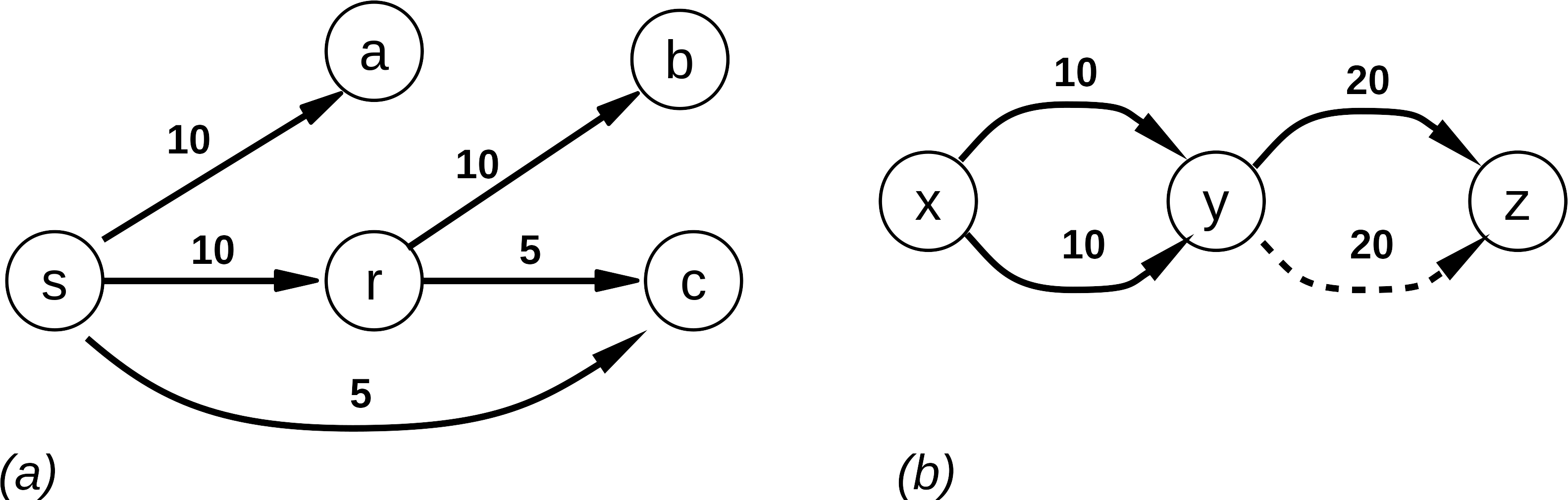
Figure 1: Sample graphs

which shows a directed graph with weighted edges. The edge weights are meant to represent a ‘strength of connection’ of the link, for example it might be the number of communication events that have taken place between the entities, number of communication modes, or the duration of such communications, some combination of both or possibly represent other factors. The only requirement is that higher edge-weight values imply a stronger connection; note that in a sense this is the opposite of edge weighting with distances where higher values imply more remoteness.

Consider the connectivity from vertex $s$ to each vertex $a$, $b$, and $c$. Intuitively, we would probably say that the $s$ to $a$ (and $r$) connection is strongest. There is a direct connection of ‘strength’ 10. Would the next strongest connection be between $s$ and $b$ or $c$? We would argue that the $s$ to $c$ connection is the next strongest because there is a direct connection of ’strength’ 5 and an indirect connection of ’strength’ 10 followed by a link of ’strength’ 5. Leaving $s$ to $b$ to be the weakest as it only has an indirect connection, even though it is through links of ’strength’ 10 and then 10. Even though there is a total connectivity of 10 from $s$ to each of $b$ and $c$, if viewed as a flow, we would likely rate the value of the direct path to $c$ as more valuable.

A hallmark of the proposed method is that outgoing edges ‘divide’ the attention of a vertex. That is the strength of connection present at a vertex is split to its out-neighbors in accordance with the numerical edge weights. These weight values could be viewed as quantification of strong and weak ties as noted in (Granovetter, 1973). As in centrality computations, we will propagate connectivity from source to destination during the calculation. A vertex’s ‘score’ (connectivity) is propagated to its neighbors according to outgoing edge weighting.

Next consider Figure 1(b). The question that arises is should the dotted edge add to the connectivity metric from $x$ to $z$? Again intuitively we would say that the connectivity from $y$ to $z$ is stronger with the dotted edge, but does (or should) its presence add to the connectivity metric from $x$? We argue that, in the nominal case where incoming connectivity strengths are summed, it should not. In this case whether $v$’s attention is divided or not, both routes land at $t$. Note that this is consistent with a similar argument from Tong et al. (2007).

Suppose there are loops in the graph; how should these impact connectivity scoring? We know that cycles have no impact on the standard path accessibility value Chebotarev and Shamis (1998), but here we argue that each outgoing edge represents a division of attention. In this case, a loop starting at a vertex should then diminish connectivity along its other outgoing paths.

These observations imply the following, that the connectivity metric should include not only shortest paths between vertices but consider all potential ‘connectivity flows’. These flows should consider the number of hops such that more remote (longer) connections, even with the same link-by-link connection strength, should not necessarily be considered equal. Cycles or loops should have impact, even though a metric like path accessibility does not.

3 A new vertex-connectivity-metric (VCM)

Our new vertex-connectivity-metric (vcm) implements the general characteristics outlined above. It also is designed to be computationally efficient, and is $O(V+E)$. As will be seen, the design forms the level graph from the source and propagates ‘connectivity’ from a given source vertex along all paths towards the destination vertex, splitting connectivity strength and modulating values by level using a given user parameter $\alpha$. This asymmetric method is applied to directed, edge-weighted graphs, but as is common, unweighted graphs can be addressed by making edge weights one and undirected graphs can be handled by placing edges in both directions.

The vcm algorithm takes as parameters the graph, $G=(V,E)$, an ‘attenuation factor’ $\alpha$, and Boolean user settings: LS level share, IM input max, and the desired source and destination vertices $s,t\in V$ for which the vcm metric is being computed. The LS parameter determines if vertices send their connectivity strength along their outedges to vertices on the same level, and IM defines that incoming connectivity strength to the next level should be the max, not sum, of incoming propagation. Typical settings might be such that the strength of connectivity is summed (IM false), exchange connectivity strength within a level (LS true) and emphasize shorter paths ($\alpha<1$). But one important distinction of the method is allowing $\alpha>1$ to emphasize, rather than de-value, longer paths.

The routine creates the level graph from $s$ with the special case that vertex $t$ is ‘moved’ to a level one higher than all the other vertices. Figure 2

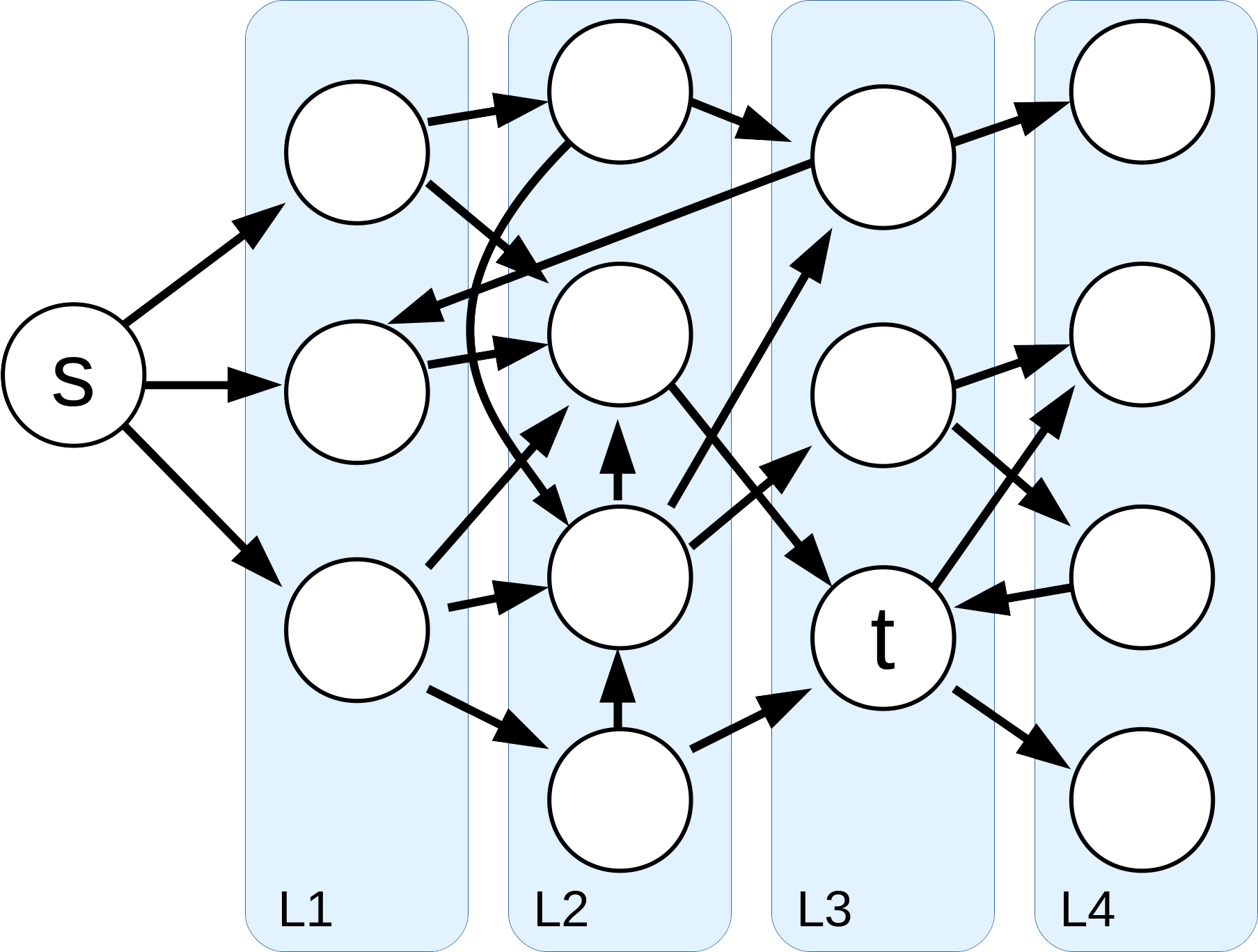
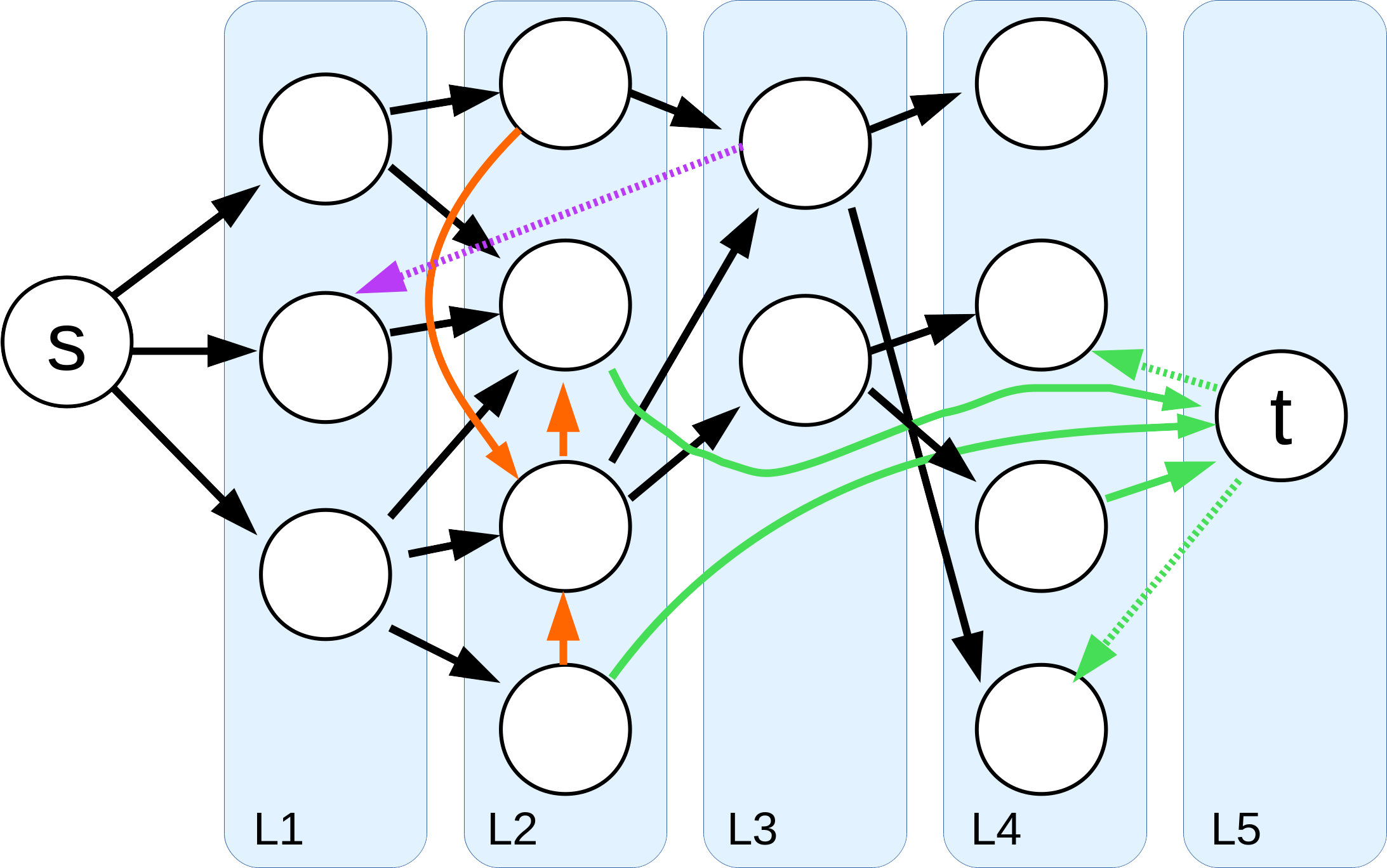
Figure 2: Level Graph Formation

illustrates this process. First the input graph is labeled in level graph form, as seen on the leftside of the figure. The target vertex $t$ is then moved to a level beyond the maximum level of all the other vertices, as seen on the rightside of the figure. This allows paths that would otherwise be from levels beyond $t$ to be included in level-by-level connectivity strength propagation to $t$. For illustrative purposes, the reverse edges (here, L3 to L1 and L5 to L4) are shown as dotted, the intra-level edges (in L2) as orange and the edges attached to $t$ in green.

Algorithm 1

Algorithm 1 The vertex-connectivity-metric method.

1:procedure vcm($s,t,\alpha$)

2:$\triangleright$ for simplicity assume $G=(V,E)$ and user settings LS, IM are global

3:     if $s=t$ then return 1 $\triangleright$ max connect to ourself      

4:     initialize $L[i]\leftarrow-1\;\;\forall i\in V$ $\triangleright$ level of each vertex

5:     initialize $W[i]\leftarrow 0.0\;\;\forall i\in V$ $\triangleright$ total weight of all edges from each vertex

6:     initialize $M[j]\leftarrow\emptyset$ $\triangleright$ set of verts on each level $j$

7:     Create level graph using BFS, setting $L,W,M$ in the process

8:     if $L[t]=-1$ then return 0 $\triangleright$ $t$ is unreachable from $s$      

9:     let $k=$ maximum level and move $t$ to level $k+1$

10:     $vcm[s]=1$

11:     for $j=0$ to $k$ do $\triangleright$ for each level

12:         if  LS  then $\triangleright$ exchange intra-level vcm strength

13:              for $v\in M[j]$ do $\triangleright$ for each vertex on level $j$

14:                  for edge $v,u$ where $L[u]=L[v]$ do $\triangleright$ $v$’s neighbors on same level

15:                       let $f=w[v,u]/W[v]$ $\triangleright$ weighting over all outedges

16:                       $vcm[u]\mathrel{+}=f\times vcm[v]$                                          

17:         let $a=\alpha^{j}$ $\triangleright$ $0^{0}=1$ here

18:         for $v\in M[j]$ do $\triangleright$ for each vertex on level $j$, propagate to higher level

19:              for edge $v,u$ where $L[u]>L[v]$ do

20:                  let $f=a\times w[v,u]/W[v]$

21:                  if  IM  then

22:                       $vcm[u]=max(f\times vcm[v],vcm[u])$

23:                  else

24:                       $vcm[u]\mathrel{+}=f\times vcm[v]$                                               

25:     return $vcm[t]$

provides an algorithm for computing vcm. The vcm metric has a maximum value of 1, and that is returned on line 2 if $s=t$ (but see later comment about the maximum exceeding 1 if $\alpha>1$). In $O(V)$ time, the level of each vertex is initialized to an ‘illegal’ value of $-1$, the total out edge weight of each vertex ($W$) is set to zero and the list of vertices on each level ($M$) is cleared (lines 3-6).

On line 6, a breadth first search is used that sets the level of each vertex (with $L[s]=0$), defines the vertex out edge weight total ($W[v]\;\forall v\in V$) and sets a list of vertices that are on each level ($M[v]$). This can be done in $O(E)$ time. On lines 8-9, $t$ is moved to past the highest level and the value of connectivity for the starting vertex is set to 1.

We then enter a level-by-level loop indexed by $j$ for each level up to $L[t]-1$. If we are doing level sharing (set by LS), then VCM scores of vertices with links on the same level (shown in orange in the figure) are propagated among each other (lines 11-15). This is scaled the same way that scores to the next level are, but is not subject to the attenuation factor, $\alpha^{j}$ defined on line 16. Next all the connectivity scores on level $j$ are propagated to the next level, subject to edge-weighting, parameter IM’s settings, and attenuation. If IM is true, then the propagated connectivity at each vertex is set to the maximum of the incoming transfers, and otherwise it’s the sum of these. The algorithm is written in a straightforward style for clarity. The routine would be implemented more efficiently by keeping separate neighbor lists from each vertex to speed the loops on lines 13 and 18.

In this design, there is no propagation along edges to lower levels (dotted edges in the figure) but their weighting is included in $W$ and diminishes forward (and intra-level) strength propagation. This does achieve the desired effect outlined in Section 2 in that loops should have impact, but does ignore longer connectivity flows that traverse levels in reverse.

Note that a non-level restricted, Katz-like but edge weighted, solution was also considered. In this case, a ‘frontier’ of vertices, possibly growing to the size of $V$, would be maintained at each step. At initialization this would include just $s,1$ (source with strength 1). At each step the frontier’s connectivity would be propagated to their neighbors, including the effects of $\alpha$, and division ala IM. After some number of steps, we would have connectivity measures to all other vertices. However, there are several issues that we would have to be overcome. Example, how would the number of steps be defined? There would be oscillation and non-convergence issues particularly, as in Katz centrality, if the $\alpha$ value permitted gain in the system. Therefore, the simpler level-based approach was devised.

Returning focus to the method, we can see that this whole routine is $O(V+E)$. The initialization and BFS routine to set $W,L,M$ is $O(V+E)$. With simple neighbor lists, the loops from lines 10-23 are $O(E)$ as all graph edges are only processed once each across all the levels $j$.

After all levels have been so processed, $\texttt{vcm}[t]$ is returned as connectivity strength from $s$ to $t$. This will be a value from 0 (weakest) to 1 (strongest), with the exception that it can exceed 1 when $\alpha>1$ (e.g., there is amplification of longer paths).

We see that this is ‘single-source/single-destination’ routine. The need to ‘move’ vertex $t$ to the outmost level in order to capture longer path contributions prevents using the method as-is for all-destination purposes. But we see that memoization techniques could be used to save prior strength propagation values for all levels below some level $k$ while doing the computations for each vertex on level $k$. That is, moving vertices from level $k$ to the level beyond the maximum does not change any computed values at levels below $k$. While this would lead to a more efficient method for an ‘single-source/all-destination’ version using dynamic programming, we leave that for future consideration.

4 Examples

For further experimentation, we have produced different outputs using two different datasets; Les-Miserablés character occurrence, and Enron email communications.

Figure 3

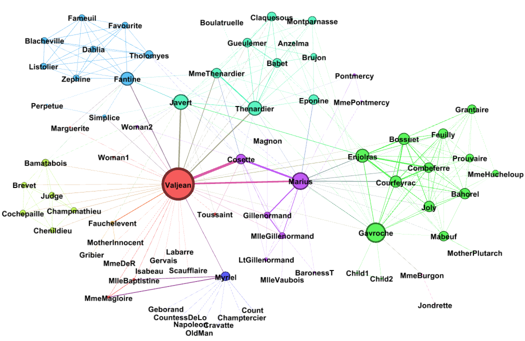
Figure 3: Les-Miserablés graph

shows the Les-Miserablés undirected network often used for network analysis demonstration. Edge weight is the count of the number of times that characters appear in the same chapter of the book; the data can be found at Carley (2021). The drawing shows vertices sized by a centrality score, which is not relevant here, but edge thicknesses are scaled with weight giving a visual clue to edge weight values.

We will apply the vcm algorithm from vertex Valjean to all other vertices for various settings of $\alpha$. For this example we will set LS true, IM false. Table 1

Table 1: Top ten VCM scoring from Valjean for Les-Miserablés graph

$\alpha\rightarrow$	0.0	0.33	0.66	1.0	1.33	1.66	2.0	2.33	2.66	3.0
1	Cos	Cos	Cos	Cos	Mar	Mar	Mar	Mar	Mar	Mar
2	Mar	Mar	Mar	Mar	Cos	Cos	Cos	Cos	Enj	Enj
3	Jav	Jav	Jav	Jav	Jav	The	The	Enj	Bos	Bos
4	The	The	The	The	The	Jav	Enj	The	Cou	Cou
5	Fan	Fan	Fan	Fan	Enj	Enj	Jav	Cou	Cos	Com
6	Fau	Mme	Mme	Mme	Mme	Mme	Cou	Bos	The	The
7	Mme	Fau	Enj	Enj	Fan	Cou	Bos	Com	Com	Gav
8	Myr	Myr	Fau	Gil	Cou	Fan	Mme	Jav	Gav	Cos
9	Enj	Enj	Myr	Fau	Gil	Bos	Com	Gav	Bla	Bla
10	Cha	Gil	Gil	Myr	Bos	Com	Fan	Mme	Fav	Fav

shows the top ten vertices (first three characters) by vcm score for each $\alpha$ value.

Typically, we would set $0\leq\alpha<1$, emphasizing stronger connections along shorter paths. But there is no requirement that $\alpha$ be set less than or equal to 1. By setting to a value greater than 1, instead of diminishing the connectivity on longer paths, we would instead enhance them. This is useful to finding relatively strong connections to more remote vertices.

At $\alpha=0$, only direct neighbors get a non-zero score, and their score is directly in accordance with the outgoing edge weights from $s$ (Valjean). In the table, we see that at $\alpha=0$, Cha (Champmathieu) is the tenth most connected to Valjean but it immediately drops off for any other $\alpha$ value. We see that Cos (Cosette) is the highest connectivity vertex until $\alpha\geq 1.33$. From visual inspection of Figure 3 we see that Cos (Cosette) is a direct neighbor of Valjean and also has the highest (thicker line) edge weight leading to its top position at lower values of $\alpha$. But at higher values of $\alpha$, Mar (Marius) becomes the strongest connection, this is becuase we are now explicitly emphasizing longer paths over shorter ones, so Mar moves into the top spot with multiple strong ties back to Valjean. Enj (Enjolras) moves from ninth strongest connection (at $\alpha=0$) to seventh at $\alpha=1$, and then to second at $\alpha=3$. Bos (Bossuet) is not in the top ten until $\alpha=1.33$ and then moves up to third place at $\alpha=3$. Thus, setting $\alpha>1$ can be seen to help find relatively strongly connected vertices that are remote, while $\alpha<1$ settings will find strong connections favoring shorter paths as is typical.

Table 2

Table 2: Top ten scoring from Valjean for other methods

				Katz measure
	comm	tong	mf	$\alpha=0.33$	$\alpha=0.66$	$\alpha=1.00$	$\alpha=2.00$
1	Gav	Cos	Mar	Jav	Jav	Jav	Jav
2	Enj	Mar	Cos	The	Gav	Gav	Gav
3	Mar	Jav	The	Gav	The	The	The
4	Bos	The	Enj	Mar	Mar	Mar	Mar
5	Cou	Enj	Com	Gue	Enj	Enj	Gue
6	Jol	Mme	Bos	Bab	Gue	Gue	Bab
7	Bah	Fan	Cou	Cla	Bab	Bab	Cla
8	The	Cou	Gav	Mme	Cla	Cla	Mme
9	Feu	Bos	Jav	Cos	Mme	Mme	Mon
10	Com	Com	Jol	Enj	Mon	Mon	Epo

shows top-ten scoring from other methods. The metric defined by Chen and Safro (2009) was also considered but it is not suitable for remote connectivity measures and is more akin to a neighbor-based similarity metric. The column comm is ‘communicability’ from Estrada and Hatano (2008). The column tong is the method from Tong et al. (2007). The column mf is max-flow, where the connectivity score is simply the max-flow value. The remaining ones are the Katz measures as defined in Cohen et al. (2012). A brief discussion of these results follows.

The ‘communicability’ Estrada and Hatano (2008) result, comm, is in the first column of Table 2. It is path count based with a value combined from the number of shortest paths and the number of longer walks, diminished by length. It does not account for edge weighting and was originally developed for community detection applications. It is the only method that puts Gav (Gavroche) as the highest connectivity (to Valjean) although the katz measures (also unweighted edges) prioritize that vertex as well.

For the Tong method (tong), a parameter ‘c’ is used to address numerical issues related to paths that cannot reach the destination and degree-1 vertices. The data in the Table uses $c=0.9$ as was also used in the reference. We see that the scoring is similar to our method, very closely following it (same first 8 entries) for $\alpha=1.3$. This method requires matrix solutions, although a means for finding all-pairs proximity with one matrix inversion is presented.

Use of maximum-flow as a connectivity measure has been offered. The scoring for that is in the mf column. One downside is that maximum-flow is flows are contentious and therefore it does not include all paths. While the value of maximum flow is unique, the flow paths to reach this value are not. In this vein, there doesn’t seem to be an easy way compose unique sets of constructive paths (via Edmonds-Karp or Dinic’s algorithms) without path enumeration (exponential). This would make it difficult to apply a path length factor such as our $\alpha$ in conjunction with flows.

The set of data in Table 2 are the ‘Katz measures’ with various $\alpha$ settings. There are obvious differences versus our method, but, as expected, perhaps more commonality with comm which is another method that does not use edge weighting. When using Katz for centrality, the $\alpha$ term must be smaller than the reciprocal of the largest eigenvector of the adjacency matrix. The metric is based on an infinite sum of walks de-rated on length against the $\alpha$ term. For the data presented in Table 2, the infinite sum was truncated to the diameter of the graph and hence should capture all non-looping walks (and looping ones that are short enough). As alluded to in the prior section, if the $\alpha$ term permits gain, this infinite sum would not converge. For the purpose here, the iteration was limited to graph diameter since we want to explore various $\alpha$ settings.

Table 3

Table 3: VCM scoring from Joly

LS true, IM true $\alpha\rightarrow$ 0.5 1.0 1.5 2.0 2.5 3.0 1 Bab 0.002 Bab 0.003 Fan 0.010 Myr 0.046 Myr 0.175 Myr 0.523 2 Bar 0.001 Fan 0.003 Myr 0.008 Fan 0.025 Fan 0.061 Fan 0.184 3 Fan 0.000 Myr 0.002 Bab 0.007 Bab 0.015 Bab 0.030 Bab 0.083 4 Myr 0.000 Bar 0.001 Bar 0.002 Bar 0.006 Bar 0.011 Bar 0.020
LS true, IM false $\alpha\rightarrow$ 0.5 1.0 1.5 2.0 2.5 3.0 1 Bab 0.003 Bab 0.015 Fan 0.058 Fan 0.230 Fan 0.745 Fan 2.050 2 Fan 0.001 Fan 0.011 Bab 0.048 Myr 0.153 Myr 0.547 Myr 1.584 3 Bar 0.001 Myr 0.005 Myr 0.032 Bab 0.125 Bab 0.294 Bab 0.642 4 Myr 0.000 Bar 0.002 Bar 0.004 Bar 0.009 Bar 0.015 Bar 0.024
LS false, IM true $\alpha\rightarrow$ 0.5 1.0 1.5 2.0 2.5 3.0 1 Bab 0.001 Bab 0.001 Fan 0.003 Fan 0.007 Myr 0.021 Myr 0.062 2 Bar 0.000 Fan 0.001 Bab 0.002 Myr 0.005 Fan 0.013 Fan 0.030 3 Fan 0.000 Bar 0.000 Myr 0.001 Bab 0.003 Bab 0.005 Bab 0.012 4 Myr 0.000 Myr 0.000 Bar 0.001 Bar 0.001 Bar 0.003 Bar 0.005
LS false, IM false $\alpha\rightarrow$ 0.5 1.0 1.5 2.0 2.5 3.0 1 Bab 0.001 Bab 0.003 Fan 0.012 Fan 0.045 Fan 0.141 Fan 0.380 2 Fan 0.000 Fan 0.002 Bab 0.010 Myr 0.025 Myr 0.089 Myr 0.254 3 Bar 0.000 Myr 0.001 Myr 0.006 Bab 0.024 Bab 0.053 Bab 0.114 4 Myr 0.000 Bar 0.001 Bar 0.001 Bar 0.002 Bar 0.004 Bar 0.006

illustrates the effect of user settings. In this case, we are considering the strength of connectivity from Joly to four others in the graph. The user controls for LS and IM are varied as is the $\alpha$ term.

If we use an $\alpha$ geared to emphasizing remote connections, e.g. column $\alpha=3$, we see that either Myr (Myriel) or Fan (Fantine) are the top choice, depending on the IM setting. If IM is true, then at each level the incoming connectivity measure to each member is the maximum stemming from the prior level. If false, then its the sum. The ‘effect’ of IM = true then is to emphasize strongest paths, although all paths are still included. While for IM = false, all paths contribute at each node as a summation. So in this case we might say that Myr (Myriel) is better connected via strongly connected paths, but Fan (Fantine) is more connected via a multitude of paths.

As a final example, Table 4

Table 4: Top ten scoring from CEO in Enron data (LS false, IM false)

level 2 vertices $\alpha\rightarrow$ 0.5 1.0 1.5 2.0 2.5 1 susan.m susan.m susan.m veronica.e veronica.e 2 sgovenar veronica.e veronica.e susan.m andrew.w 3 miyung.b sgovenar cheryl.j cheryl.j henry.e 4 tammie.s miyung.b tana.j tana.j cheryl.j 5 james.s james.s miyung.b sara.s robert.e 6 kimberly.h tana.j sgovenar andrew.w sara.d 7 veronica.e tammie.s james.s henry.e tana.j 8 sharron.w cheryl.j sara.s sara.d sara.s 9 christi.n kimberly.h janette.e robert.e susan.m 10 donna.l janette.e tammie.s miyung.b all.w
level 3 vertices $\alpha\rightarrow$ 0.5 1.0 1.5 2.0 2.5 1 sap.h sap.h sap.h pramath_s pramath_s 2 ernest.o ernest.o ernest.o msorrell msorrell 3 public.r public.r msorrell smu-betas smu-betas 4 leo.w leo.w pramath_s hhabicht hhabicht 5 ken.s pfranz public.r halperin halperin 6 pfranz ken.s leo.w doyle doyle 7 traders.e traders.e smu-betas bstephen bstephen 8 center.e center.e jami.h jami.h yolanda 9 houston.p houston.p pfranz sap.h jpainter 10 jeffrey.s jeffrey.s ken.s ernest.o spikesp
level 4 vertices

$\alpha\rightarrow$	0.5	1.0	1.5	2.0	2.5
1	stebbins.j	ken_lay	ken_lay	jpfloom	jpfloom
2	ken_lay	stebbins.j	jpfloom	jmoriarty	jmoriarty
3	canada.d	canada.d	jmoriarty	primlmates	primlmates
4	enron.c	enron.c	canada.d	jgosar	jgosar
5	add…_ena…	add…_ena…	enron.c	ken_lay	20participants
6	glenn.d	glenn.d	add…_ena…	20participants	christine.m
7	executive.l	executive.l	jgosar	christine.m	dave.d
8	rcunningham	rcunningham	primlmates	dave.d	s20761
9	mmccoy	mmccoy	glenn.d	mgp427	p10621
10	sdaniel	sdaniel	executive.l	s20761	plemme

provides top ten scoring using the Enron email dataset as defined in Shetty and Adibi (2004). This data has vertices that are email addresses and edges that are emails between these addresses. There are over 2M emails that simplify to 583,550 pairwise (simple) weighted graph edges between 75,153 vertices. The emails are directed as sender and receiver, however we consider the graph to be undirected here. Of course, there can be multiple emails between two parties, and this count is used as the edge weight. We could also consider factoring in the email size to compose a more complex edge weighting scheme, but that is left for future consideration.

For this experiment, we are studying the connectivity from the CEO (Jeff Skilling) to those that are not in direct contact with him. The first table shows the top ten scores among the set of vertices that are 2 steps away (e.g., level=2), the next 3 steps and finally 4 steps. At level=2, there are 15,724 vertices. At level=3, there are 35,389 vertices and at level=4, there are 19,080 vertices. These tables show the best connected vertices remote from the source (Skilling) at given levels (also varied against the $\alpha$ term).

5 Concluding Remarks

A new vertex connectivity metric has been developed and demonstrated. While geared towards social networks, the metric is general in nature leveraging only graph structure and weighting. The method ‘propagates’ connectivity strength values within and to higher levels in the level-graph image of the input graph. As loops are avoided, but penalized, this allows exploration of both gain and loss settings against path length.

A summary of its features is:

• Leverages edge weighting as a strength of connection value

• Applicable to directed or undirected graphs

• Level reverse/looping paths are not explicitly included, but a penalty is imposed for level-reverse edges

• Path length factors to prioritize either shorter (typical) or longer paths

• Efficient, $O(V+E)$ – does not require matrix solution/inversion.

References

- Doreian [1974] Patrick Doreian. On the connectivity of social networks. J. Mathematical Sociology, 3:245–258, 1974.
- Ding and Dixon [2008] Li Ding and Brandon Dixon. Using an edge-dual graph and -connectivity to identify strong connections in social networks. In Proc. 46th ACM Southeast Regional Conf. , pages 475–480, Auburn, AL, March 2008.
- Cohen et al. [2012] Sara Cohen, Benny Kimelfeld, and Georgia Koutrika. A survey on proximity measures for social networks. Lecture Notes in Computer Science (LNCS), pages 191–206, January 2012.
- Chebotarev and Shamis [1998] P. Yu Chebotarev and E.V. Shamis. On proximity measures for graph vertices. Automation and Remote Control, 59(10):1443–59, 1998.
- Chierichetti et al. [2010] Flavio Chierichetti, Silvio Lattanzi, and Alessandro Panconesi. Rumour spreading and graph conductance. In Proc. 21st ACM-SIAM Symp. Discrete Algorithms (SODA’10), pages 1657–1663, Philadelphia, PA, January 2010.
- Sinclair [1993] Allstair Sinclair. Algorithms for Random Generation and Counting: a Markov Chain Approach. Birkhauser-Verlag, Basel, Switzerland, January 1993.
- Censor-Hillel and Shachnai [2012] Keren Censor-Hillel and Hadas Shachnai. Fast information spreading in graphs with large weak conductance. SIAM J. Computing, 41(6):1451–1465, 2012.
- Tong et al. [2007] Hanghang Tong, Yehuda Koren, and Christos Faloutsos. Fast direction-aware proximity for graph mining. In Proc. 13th ACM Knowledge Discovery and Data (KDD’07), Aug 12–15 2007. San Jose, CA.
- Faloutsos et al. [2004] Christos Faloutsos, Kevin McCurley, and Andrew Tomkins. Fast discovery of connection subgraphs. In Proc. 10th ACM Knowledge Discovery and Data (KDD’04), pages 118–127, Aug 2004. Seattle, WA.
- Xu and Chen [2004] Jennifer Xu and Hsinchun Chen. Fighting organized crime: using shortest path algorithms to identify associations in criminal networks. Decision Support Systems, 38:473–487, 2004.
- Newman [2018] Mark Newman. Networks. Oxford University Press, 2018.
- Barnes [1969] J. A. Barnes. Graph theory and social networks: A technical comment on connectedness and connectivity. Sociology, 3(2):215–232, May 1969.
- Martino and Spoto [2006] Francesco Martino and Andrea Spoto. Social network analysis: A brief theoretical review and further perspectives in the study of information theory. PsychNology Journal, 4(1):53–86, 2006.
- Granovetter [1973] Mark Granovetter. The strength of weak ties. Amer. J. Sociology, 78(6):1360–1380, May 1973.
- Carley [2021] Kathleen Carley. Center for computational analysis of social and organizational systems (CASOS). http://casos.cs.cmu.edu, 2021.
- Chen and Safro [2009] Jie Chen and Ilya Safro. A Measure of the Connection Strength Between Graph Vertices with Applications. arXiv e-prints, September 2009. arXiv:0900.4275.
- Estrada and Hatano [2008] Ernesto Estrada and N. Hatano. Communicability in complex graphs. Physical Review E, 77(3), March 2008.
- Shetty and Adibi [2004] Jitesh Shetty and Jafar Adibi. The Enron email dataset: Database schema and brief statistical report. Technical report, January 2004.