Calibration of a SEIR–SEI epidemic model to describe
the Zika virus outbreak in Brazil

Abstract

Multiple instances of Zika virus epidemic have been reported around the world in the last two decades, turning the related illness into an international concern. In this context the use of mathematical models for epidemics is of great importance, since they are useful tools to study the underlying outbreak numbers and allow one to test the effectiveness of different strategies used to combat the associated diseases. This work deals with the development and calibration of an epidemic model to describe the 2016 outbreak of Zika virus in Brazil. A system of 8 differential equations with 8 parameters is employed to model the evolution of the infection through two populations. Nominal values for the model parameters are estimated from the literature. An inverse problem is formulated and solved by comparing the system response to real data from the outbreak. The calibrated results presents realistic parameters and returns reasonable descriptions, with the curve shape similar to the outbreak evolution and peak value close to the highest number of infected people during 2016. Considerations about the lack of data for some initial conditions are also made through an analysis over the response behavior according to their change in value.

1 Introduction

The Zika virus is a flavivirus that upon infection in humans causes an illness, known as Zika fever, identified commonly with macular or papular rash, mild fever and arthritis [1, 2]. It is mainly a vector-borne disease carried by the genus Aedes of mosquitoes [2, 3], while in a lesser amount it is also transmitted via sexual interaction [4, 5], and contamination by blood transfusion is under investigation [6]. The Zika virus was first isolated in primates from the Zika forest in Uganda in $1947$ [7]. Evidences of the virus in humans were found in Nigeria in $1968$ [8]. An epidemic occurred in $2007$ on Micronesia [9], followed by multiple outbreaks on several Pacific Islands between $2013$ and $2014$ [10, 11]. The first Zika virus autochthonous case in Brazil was reported around April, $2015$ [12], and nearly $30{,}000$ cases of infection were already notified by January $30$, $2016$ [13], along with the Pan American Health Organization being informed in the same month about locally-transmitted cases on numerous continental and island territories of America [14]. The Brazilian Ministry of Health registered $215{,}319$ probable cases of Zika fever ($130{,}701$ of which were confirmed) until the $52$th epidemiological week (EW) of $2016$ [12]. The Zika epidemic has been causing concern in the international medical community, health authorities and population, specially due to an association between the Zika virus and other diseases, such as newborn microcephaly [4, 15] and Guillain-Barré syndrome [16], whose correlation to the Zika virus was considered by the World Health Organization a “scientific consensus” [17].

In this epidemic scenario, the development of control and prevention strategies for the mass infection is a critical issue. A mathematical model capable of providing a description of the infected people throughout an outbreak is a useful tool that can be employed to identify effective and vulnerable aspects on disease control programs [18, 19, 20]. Furthermore, for an epidemic model to be truly useful it must undergo a judicious process of validation [21, 22], which consists in comparing model predictions with real data in order to evaluate if they are realistic. In general, the first predictions of a model do not agree with the observations, possibly due to inadequacies in the model hypotheses or because of a poor choice for the model nominal parameters. The first case invalidates the model, but the second can be amended through a procedure known as model calibration, where a set of parameters that promote a good agreement between predictions and observations is sought.

This work is one of the results in a rigorous ongoing process of identification and validation of representative models to describe Zika virus outbreaks in Brazil [23, 24]. For this purpose, a SEIR-SEI mathematical model is adapted to the Brazilian scenario. This specific SEIR-SEI description has been successfully used before for the outbreaks in Micronesia [25] and French Polynesia [26]. Some assumptions were also based on similar studies performed over SEIR dynamical systems [27, 28, 29, 30]. The nominal values of the model parameters belong to characteristics of the Zika infection and its vector, quantitatively estimated in the literature or published by health organizations. Predictions are obtained from numerical simulation and further heuristic manipulation, followed by a comparison to real data of the outbreak as an initial effort to validate the model. In sequence, a rigorous process of model calibration is performed through the formulation and solution of an inverse problem.

The rest of this paper is organized as follows. In section 2, the mathematical model is described and estimation of nominal values for the model parameters is discussed. In section 3, the forward and inverse problems are formulated and solved, where results are detailed and a subsequent comparison between model predictions and experimental data is made to calibrate the model. Finally, in section 4, the main contributions of this work are emphasized and a path for future works is suggested.

2 Epidemic model for Zika virus dynamics

2.1 Model hypotheses

This work utilizes a variant of the Ross-Macdonald model [31] for epidemic predictions, separating the populations into a SEIR-SEI framework (susceptible, exposed, infectious, recovered) [32, 33, 34]. Each category represents the health condition of an individual inside such group at time $t$, with respect to the considered infection. The susceptible group, denoted by $S(t)$, represents those who are uncontaminated and are able to become infected. The exposed portion of the population, $E(t)$, comprehends anyone that is carrying the pathogen but is still incapable of transmitting the disease. While the infectious individuals, $I(t)$, can spread the pathogen and may display symptoms associated with the illness. Finally, the recovered group, $R(t)$, contains those who are no longer infected. The populations of humans and vectors are segmented into the aforesaid classes (excepting the group of recovered vectors), as Figure 1 depicts schematically with the accordingly subscripts. $S_{h}$, $E_{h}$, $I_{h}$ and $R_{h}$ amass the number of people at each stage of the model description, and $S_{v}$, $E_{v}$, $I_{v}$ signifies proportion of vectors ($0\leq S_{v},\,E_{v},\,I_{v}\leq 1$ and $S_{v}+E_{v}+I_{v}=1$).

Figure 1: Schematic representation of the SEIR–SEI model for the Zika virus outbreak description.

Demographic changes in the number of humans are not considered because the timescale of infection is much faster than the timescale of birth and deaths for the latter to significantly alter the development of the disease in the Brazilian context (supplementary material B provides tools to test this assertion). The total vector population is maintained constant during the analysis, although variations of the proportion of vectors on the particular compartments are introduced via birth and death rates. The vector in question is regarded as a hypothetical mosquito apt to being infected or infectious throughout all its lifetime — which means the model accounts only for the adult stage of their life cycle — and also unable to recover.

The time elapsed while an individual is on the aforementioned exposed group is known as the latent period of an organism and, in this work, is adopted as equivalent to the commonly called incubation period (the time elapsed between being infected and exhibiting symptoms), since data is extremely sparse on the latter for humans [35] (namely, the intrinsic incubation period). Both terms are used interchangeably hereafter, and the concepts do not differ on the mosquitoes case (the extrinsic incubation period) [36]. In addition, all the members of the susceptible group are treated as equally capable of being infected and the recovered ones as completely immunized.

2.2 Model equations

The evolution of individuals through the SEIR-SEI groups is governed by the following (nonlinear) autonomous system of ordinary differential equations

$$\mathinner{\dfrac{\operatorname{d\!}{}S_{h}}{\operatorname{d\!}{t}}} =-\beta_{h}\,S_{h}\,\frac{I_{v}}{N_{v}}\>, \mathinner{\dfrac{\operatorname{d\!}{}S_{v}}{\operatorname{d\!}{t}}} =\delta\,N_{v}-\beta_{v}\,S_{v}\,\frac{I_{h}}{N_{h}}-\delta\,S_{v}\>,$$ (1)

$$\mathinner{\dfrac{\operatorname{d\!}{}E_{h}}{\operatorname{d\!}{t}}} ={\beta_{h}}\,S_{h}\,\frac{I_{v}}{N_{v}}-\alpha_{h}\,E_{h}\>, \mathinner{\dfrac{\operatorname{d\!}{}E_{v}}{\operatorname{d\!}{t}}} =\beta_{v}\,S_{v}\,\frac{I_{h}}{N_{h}}-(\alpha_{v}+\delta)\,E_{v}\>,$$

$$\mathinner{\dfrac{\operatorname{d\!}{}I_{h}}{\operatorname{d\!}{t}}} =\alpha_{h}\,E_{h}-\gamma\,I_{h}\>, \mathinner{\dfrac{\operatorname{d\!}{}I_{v}}{\operatorname{d\!}{t}}} =\alpha_{v}\,E_{v}-\delta\,I_{v}\>,$$

$$\mathinner{\dfrac{\operatorname{d\!}{}R_{h}}{\operatorname{d\!}{t}}} =\gamma\,I_{h}\>, \mathinner{\dfrac{\operatorname{d\!}{}C}{\operatorname{d\!}{t}}} =\alpha_{h}\,E_{h}\>,$$

where $N$ represents the total population and $1/\!\alpha$ the disease’s incubation period (each with the corresponding subscript of $h$ for human’s and $v$ for vector’s), $1/\!\delta$ means the vector lifespan, $1/\!\gamma$ is the human infection period — which is defined in this work as the interval of time that a human is infectious — and $\beta$ identifies the transmission rate, specifically $\beta_{h}$ is the mosquito-to-human rate and $\beta_{v}$ the human-to-mosquito rate.

The transmission terms $\beta_{h}\,S_{h}\,I_{v}/N_{v}$ and $\beta_{v}\,S_{v}\,I_{h}/N_{h}$ are composed by a number of susceptible individuals ($S_{h},\,S_{v}$, respectively), a transmission rate ($\beta_{h},\,\beta_{v}$) and the probability of the contact being made with an infectious member of the other population ($I_{v}/N_{v},\,I_{h}/N_{h}$). Both transmissions terms come from the assumption that the rate of contacts is constant, which characterizes a frequency-dependent transmission [37].

The compartmentalization hypothesis requires setting the variables at the initial time of the analysis, $t_{0}$, such that their sum equals the total population in each case, e.g, $S_{v}(t_{0})+E_{v}(t_{0})+I_{v}(t_{0})=N_{v}=1$. By so doing, for all $t>t_{0}$, $S_{h}(t)$, $E_{h}(t)$, $I_{h}(t)$ and $R_{h}(t)$ will always add up to $N_{h}$; and $N_{v}(t)$ will be the equilibrium solution of the initial value problem

$$\mathinner{\dfrac{\operatorname{d\!}{}N_{v}}{\operatorname{d\!}{t}}} =\delta\,(1-N_{v}(t))\>, N_{v}(t_{0})=1\>,$$ (2)

namely, $N_{v}(t)=1$. This consideration allows the simplification of treating the total vector population as a parameter $N_{v}$, instead of a variable, since it stays constant throughout the analysis. If one wishes to treat the vector population as a variable, a recruitment parameter would need to be added in place of $\delta\,N_{v}$ as well as another differential equation to account for the changes in $N_{v}(t)$.

The $\operatorname{d\!}C/\!\operatorname{d\!}t$ equation allows evaluation of the cumulative number $C(t)$ of infectious people until the time $t$, that is, the amount of humans so far that contracted the disease and have passed through or are in the infectious group at the given time.

Additionally, a set of $M=52$ points to represent the number of new infectious cases of Zika fever at each week is defined as follows:

$$\mathcal{N}_{w}=C_{w}-C_{w-1}\>,\quad\mathcal{N}_{1}=C_{1},\leavevmode\nobreak\ \leavevmode\nobreak\ w=2,\cdots,52\>,$$ (3)

where $C_{w}$ is the cumulative number of infectious humans in the w-th EW.

Figure 2 organizes the data of cumulative number of infectious and new cases per week provided by the Brazilian Ministry of Health [38] (supplementary material A) for 2016, where the evolution of the infection can be seen.

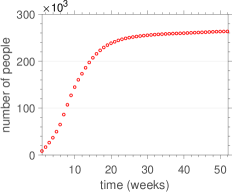
(a) Cumulative number

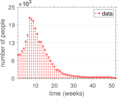
(b) New cases

Figure 2: Outbreak data.

The expected behavior for the model is that it generates a seemingly year long outbreak for 2016 that matches $C(t)$ and $\mathcal{N}_{w}$ to the data of Figure 2. The end of this outbreak is marked by the exposed and infectious portions of vectors reaching very low values, effectively killing off the contamination process to the point that $S_{h}(t)$ stabilizes.

2.3 Nominal parameters

The preliminary values for the parameters of the set of Eqs. (1) come from the related literature concerning the Zika infection, vector-borne epidemic models, the Aedes aegypti mosquito (which is the main vector for Zika, Dengue and Yellow fever in Brazil) and publications provided by health organizations and government agencies. The Brazilian Institute of Geography and Statistics reports that Brazil had approximately $N_{h}=206\times 10^{6}$ people by July, $2016$ [39], and $N_{v}$ is set $1$ to entail an entire vector population. The adopted extrinsic incubation period is $1/\!\alpha_{v}=9.1$ days [25]. This value agrees with other statistical confidence intervals (CI) that are presented for the parameter in another works ($95$% CI: $7.3$–$9.3$ days [40]) and is close to the numbers suggested by experimental studies for the time necessary for the virus to reach the mosquito’s saliva after an infectious blood meal ($5$ [41, 42] and $7$ days [43]). A systematic review and pooled analysis of the literature and case studies available in [44] estimates that the median intrinsic incubation period is $5.9$ days ($95$% CI: $4.4$–-$7.6$). This values is selected for $1/\!\alpha_{h}$ in this work and is compatible with the range of $3$–$12$ days recommended by multiple sources [15, 45, 46], also formerly used in previous studies [47]. The aforementioned literature analysis in [44] also concludes that $9.9$ ($95$% CI: $6.9$-–$21.4$) days is the mean time until an infected has no detectable virus in blood. Considering the assumption that the infectiousness in Zika infection ends $1.5$–$2$ days before the virus becomes undetectable [25, 40], the chosen value for the human infectious period is $1/\!\gamma=9.9-2=7.9$ days. As for the vector lifespan $1/\!\delta$, “the adult stage of the mosquito is considered to last an average of eleven days in the urban environment" according to [48]. This is the assumed value for the parameter in this work, which is also consistent with the usual life expectancy for the mosquito in Rio de Janeiro, Brazil [49], and comes close to the average of $2$–$3$ weeks considered in biological studies about the species [50] and by the Centers for Disease Control and Prevention [51]. Lastly, the time between a mosquito being infected and it infecting a human, $1/\!\beta_{h}$, and the time between a human infection and a mosquito taking an infectious blood meal, $1/\!\beta_{v}$, is estimated in [40] as an average of $11.3$ days ($95$% CI: $8.0$–$16.3$) and $8.6$ days ($95$% CI: $6.2$-$11.6$), respectively.

3 Calibration of the epidemic model

3.1 Forward Problem

The epidemic model of section 2, supplemented by an appropriate set of initial conditions, is a continuous-time dynamical system

$$\dot{\mathbf{x}}(t)=\mathbf{f}\left(\mathbf{x}(t),\mathbf{p}\right)\>,\quad\mathbf{x}(t_{0})=\mathbf{x}_{0}$$ (4)

where $\mathbf{x}(t)=\left(S_{h}(t),E_{h}(t),I_{h}(t),R_{h}(t),S_{v}(t),E_{v}(t),I_{v}(t),C(t)\right)\in\mathbb{R}^{8}$ is the vector of states at time $t$, $\mathbf{x}_{0}=\left(S_{h}^{i},E_{h}^{i},I_{h}^{i},R_{h}^{i},S_{v}^{i},E_{v}^{i},I_{v}^{i},C^{i}\right)\in\mathbb{R}^{8}$ is a prescribed initial condition vector referring to the initial time $t_{0}$ of the analysis, the vector $\mathbf{p}=\left(N_{h},\beta_{h},\alpha_{h},\gamma,N_{v},\beta_{v},\alpha_{v},\delta\right)\in\mathbb{R}^{8}$ lumps the model parameters and $\mathbf{f}\mathrel{\mathop{\mathchar 58\relax}}U\subset\mathbb{R}^{8}\times\mathbb{R}^{8}\to\mathbb{R}^{8}$ is a nonlinear map which gives the evolution law of this dynamics, defined (for fixed $t$) on the open set

$$U=\left\{(\mathbf{x}(t),\mathbf{p})\in\mathbb{R}^{8}\times\mathbb{R}^{8}\leavevmode\nobreak\ \big{|}\leavevmode\nobreak\ x_{n}(t)>0\leavevmode\nobreak\ \mbox{and}\leavevmode\nobreak\ p_{n}>0,\leavevmode\nobreak\ \mbox{for}\leavevmode\nobreak\ n=1,\cdots,8\right\}.$$ (5)

The forward problem consists in providing initial conditions (IC) and a set of parameters, represented by the pair $\bm{\alpha}=(\mathbf{x}_{0},\mathbf{p})$, and compute by means of numerical integration the model response $\mathbf{x}(t)$ from which a scalar observable $\bm{\phi}(\bm{\alpha},t)$ is obtained. In the forward problem, $\bm{\alpha}$ represents all IC and system parameters from Eq.(1), while $\bm{\phi}(\bm{\alpha},t)$ is the new cases $\mathcal{N}_{w}$ system response from Eq.(3).

Since the map $\mathbf{f}$ has a polynomial nature in $\mathbf{x}$, it is a continuously differentiable function in $\mathbf{x}$. Thus, the existence and uniqueness theorem for ordinary differential equations guarantees that the initial value problem of (4) has an unique solution. Besides that, one can also show that this solution is continuously dependent on $\bm{\alpha}$, as well as the forward map $\bm{\phi}$ [52, 53].

The evaluation of the system response in the forward problem is performed numerically in this work via a Runge-Kutta (4,5) method and the scalar observable of interest $\mathcal{N}_{w}$ is used to assess the simulation when compared with real data of the 2016 outbreak made available by the Brazilian Ministry of Health [38] (supplementary material A). The referred data consists of probable cases of infected people per EW, registered by sanitary outposts and health institutions throughout the country when the common symptoms of Zika fever were exhibited by an individual. In accordance with the hypothesis that one only displays symptoms when inside $I_{h}(t)$, the $C(t)$ variable models this discrete accumulating data on a continuous sense and $\mathcal{N}_{w}$ provides the corresponding influx per EW. The $C(t)$ time series is also observed as a criteria for good fitting, since it signifies the general impact of the epidemic and because a reasonable $\mathcal{N}_{w}$ result does not necessarily implies an acceptable cumulative number of infectious individuals for all $t$ in comparison to the data.

The initial time of the analysis was established as the first EW of 2016. The remaining individuals in both populations are assumed susceptible at first, meaning $S_{h}^{i}=N_{h}-E_{h}^{i}-I_{h}^{i}-R_{h}^{i}$ and $S_{v}^{i}=N_{v}-E_{v}^{i}-I_{v}^{i}$. The initial values for the exposed and infectious groups are set equal, $E_{h}^{i}=I_{h}^{i}$ and $E_{v}^{i}=I_{v}^{i}$. Likewise, the number of infected humans at the initial time must be $I_{h}^{i}=C^{i}$, given its definition. The value of $C^{i}$ is taken as the number of confirmed Zika cases in Brazil on the first EW of $2016$ [38], $8{,}201$ individuals, and the recovered group is assumed equal to the suspected number of infected in $2015$, according to the data available [13], $R_{h}^{i}=29{,}639$ individuals. As for the proportion of infectious vectors in the first week, to work around the lack of data for this initial condition, repetitive manual estimations were tried until the resulted time series of $\mathcal{N}_{w}$ presented reasonable values compared to the real data. It became clear that the system response is very sensible to $I_{v}^{i}$, as slight variations in its value are required to achieve feasible results. In the process of choosing its value, the matching of the $\mathcal{N}_{w}$ curve’s peak to the amplitude of infection is also a priority, since this is the main interest region for evaluation of the outbreak. The nominal values of the parameters exhibited viable $\mathcal{N}_{w}$ curves around $I_{v}^{i}=2.2\times 10^{-4}$.

Figure 3 presents the SEIR-SEI model response for the nominal set of parameters from section 2.3, supplied with the above IC, on an epidemiological week temporal domain consisting of one to fifty-two weeks ($7$ to $365$ days), compared with the data of the outbreak (red dots).

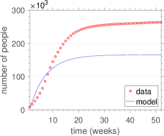
(a) Cumulative number

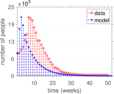
(b) New cases

Figure 3: Outbreak data (red) and model response using the nominal parameters (blue).

The general shape of the curves in Figure 3 do provide qualitative information regarding the evolution of the infection, even though the portrayed descriptions are not quantitatively realistic. This inherent pattern agreement and numerical mismatch suggests that the model response may differ from the real data due to the use of unsuitable values for the parameters or incorrect IC assumptions. The search for parameter and initial condition values that make the simulations fit well to the observed data defines model calibration (or system identification), being the object of interest of the next section.

3.2 Inverse Problem

The model calibration problem seeks to find a set of parameters that, to a certain degree, makes the model response as close as possible to the empirical observations (reference data), once, due to the erros on model conception and reference data acquisition, it is (practically) impossible for the forward map to reproduce the outbreak observations.

The mathematical setting for this case considers the parameters vector $\bm{\alpha}$ defined in the parameter space $E=\mathbb{R}^{12}$, since here $\bm{\alpha}$ comprises all IC and system parameters from Eq.(1) , excepting $N_{h}$, $N_{v}$, $R_{h}^{i}$ and $C^{i}$, which are kept fixed in their nominal values. For the purpose of comparison between observations and predictions, a discrete set with $M$ time-instants is considered, so that scalar observations and predictions are respectively lumped into $\bm{y}=(y_{1},y_{2},\cdots,y_{M})$ and $\bm{\phi}\left(\bm{\alpha}\right)=\left(\phi_{1},\phi_{2},\cdots,\phi_{M}\right)$, both defined in the data space $F=\mathbb{R}^{M}$. Note that the forward map $\bm{\phi}\mathrel{\mathop{\mathchar 58\relax}}E\to F$ associates to each parameters vector $\bm{\alpha}$ an observable vector $\bm{\phi}\left(\bm{\alpha}\right)$ where the component represents the number of new cases in each week of the year, i.e., $\bm{\phi}_{w}=\mathcal{N}_{w}$. In practice, the parameters vector is restricted to be on the convex set of admissible values $C=\left\{\bm{\alpha}\in E\leavevmode\nobreak\ \big{|}\leavevmode\nobreak\ \textbf{lb}\,\leq\bm{\alpha}\leq\,\textbf{ub}\right\}$, in which lb and ub are lower and upper vector bounds for $\bm{\alpha}$, respectively.

In formal terms, given an observation vector $\bm{y}\in F$ and a prediction vector $\bm{\phi}\left(\bm{\alpha}\right)\in F$, the calibration aims at finding a vector of parameters $\bm{\alpha}^{\ast}$ such that

$$\bm{\alpha}^{\ast}=\operatorname*{arg\,min}_{\bm{\alpha}\in C}\,J(\bm{\alpha})\>,$$ (6)

for a misfit function

$$J(\bm{\alpha})=||\bm{y}-\bm{\phi}\left(\bm{\alpha}\right)||^{2}=\left\{\sum_{m=1}^{M}\Big{|}y_{m}-\phi_{m}\left(\bm{\alpha}\right)\Big{|}^{2}\right\}.$$ (7)

This is the inverse problem associated to the epidemic model. In general this type of problem is extremely nonlinear, with none or low regularity, multiple solutions (or even none), being much more complicated to attack in comparison with the forward problem [54, 55]. A schematic representation of the forward and the inverse problem associated to the epidemic model is shown in Figure 4.

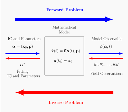
Figure 4: Schematic representation of the forward and inverse problems associated to the epidemic model.

This inverse problem attempts to estimate a finite number of parameters on a finite dimension space, being defined in terms of a typical nonlinear misfit function. Therefore, Theorem 4.5.1 of [56] can be invoked to guarantee a proper sense of well-posedness (existence, uniqueness, unimodality and local stability) for the inverse problem.

The Trust-Region-Reflective method (TRR) is employed here to numerically approximate a solution for the inverse problem (6). The main idea of the method is to minimize a simpler function that reflects the behavior of $J(\bm{\alpha})$ in a neighborhood (trust-region) around $\bm{\alpha}$. The simpler function is defined as dependent on the trial step $\mathbf{s}$, characterizing the Trust-Region subproblem, and its computation is optimized by restricting the subproblem to a two-dimensional subspace. The subspace is linear spanned by a multiple of the gradient $\mathbf{g}$ and (in the bounded case) a vector obtained in a scaled modified Newton step, used for the convergence condition ${D(\bm{\alpha})}^{-2}\,\mathbf{g}(\bm{\alpha})=0$, where $D$ is a diagonal matrix that depends on $\bm{\alpha}$, $\mathbf{g}$, $\mathbf{lb}$, and $\mathbf{ub}$ [57]. Finally, the trial step is found through the subproblem as

$$\mathbf{s^{*}}=\operatorname*{arg\,min}_{\mathbf{s}}\left\{\frac{1}{2}\mathbf{s}^{\mathrm{\!T}}Q\mathbf{s}+\mathbf{g}^{\mathrm{\!T}}\mathbf{s}\>\mid\>{||D\,\mathbf{s}||}_{2}\leq\Delta\right\}\>,$$ (8)

where $\Delta$ is a scalar associated with the trust region size; $Q$ is a matrix involving $D$, a Jacobian matrix (also dependent on $\bm{\alpha}$, $\mathbf{g}$, $\mathbf{lb}$, and $\mathbf{ub}$) and an approximation of the Hessian matrix [57]. The quadratic approximation in Eq.(8) has well-behaved solutions [58] and if $J(\bm{\alpha}+\mathbf{s})<J(\bm{\alpha})$ then $\bm{\alpha}$ is updated to $\bm{\alpha}+\mathbf{s}$ and the process iterates, otherwise $\Delta$ is decreased. In addition, a reflection step also occurs if a given step intersects a bound: the reflected step is equivalent to the original step except in the intersecting dimension, where it assumes the opposite value after reflection.

The TRR algorithm also requires an initial guess for each parameter, identified in the next section as “TRR input”. The stopping criteria are the norm of the step and the change in the value of the objective function, with a tolerance of $10^{-7}$. Supplementary material B provides details on the software used for implementation.

3.3 Numerical experiments for calibration

Figure 5 presents the best result for the $\mathcal{N}_{w}$ system response fitting problem using the nominal parameters and IC from sections 2.3 and 3.1 as initial guesses for the TRR algorithm. The upper and lower bounds used for the parameters were set compatible with the literature suggested intervals and are presented in Table 1, along with the parameters and IC values resulted from the calibration (“TRR output”). The $\mathbf{ub}$ for $\delta$ was assumed lower than the $\mathbf{lb}$ for $\alpha_{v}$ to maintain consistency with the model interpretation. The minima for $S_{h}^{i}$ and $S_{v}^{i}$ were set to $0.9\,N_{h}$ and $0.99$, respectively, to establish a high number of susceptible individuals as is expected for the beginning of an outbreak. Also, the lower and upper bound ($0.999$) for $S_{v}^{i}$ were motivated by noticing how variations in $E_{v}^{i}$ and $I_{v}^{i}$ of order $10^{-3}$ already bring significant changes in the system response. The lack of available data for the exposed and infectious groups at the onset of the epidemic was circumvented by appointing its minimum and maximum possible values as $\mathbf{lb}$ and $\mathbf{ub}$, i.e., $E_{v}^{i}$ and $I_{v}^{i}$ were restricted between zero and one, while $E_{h}^{i}$ and $I_{h}^{i}$ were bounded by zero and $N_{h}$.

Additionally, to ensure the model hypotheses of compartmentalization and constant population, two additional fitting points were defined, $\Sigma_{h}=S_{h}^{i}+E_{h}^{i}+I_{h}^{i}$ and $\Sigma_{v}=S_{v}^{i}+E_{v}^{i}+I_{v}^{i}$, which were set to match $N_{h}-R_{h}^{i}$ and $N_{v}=1$ on Eq.(6), respectively. However, the algorithm is only capable of approximating $\Sigma_{h}$ and $\Sigma_{v}$ to their intended values. So to account for these minor differences, the resulting values of $(N_{h}-R_{h}^{i})-\Sigma_{h}$ and $1-\Sigma_{v}$ were added to the TRR output of $S_{h}^{i}$ and $S_{v}^{i}$. These corrections did not impact the calibration, since the scale of the differences would always be, correspondingly, $10^{-4}$ and $10^{-2}$ (at most), which are below the sensibility of $S_{h}^{i}$ and $S_{v}^{i}$; thus, they were only exacted to keep the hypotheses rigorously sustained, otherwise the sum of the compartments in each population would quickly tend to $N_{h}$ and $N_{v}$ in an asymptotic fashion.

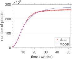
(a) Cumulative number

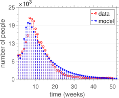
(b) New cases

Figure 5: Outbreak data (red) and calibrated model response (blue) from Table 1.

Clearly, Figure 5 is a reasonable description of the outbreak: the general shape of the infection evolution is attained, all parameters are within realistic possibilities, the $C(t)$ curve overshoots the data by merely $6.00\%$, the peak value of $\mathcal{N}_{w}$ differs from the empirical data maximum by $7.87\%$ and is only one week off. However, taking into consideration the order of magnitude of the first data point ($C^{i}=8{,}201$) and the scale of the infection ($215{,}319$ probable cases until the $52$th EW [12]), the TRR output for $I_{h}^{i}$ ($253{,}360$) is probably too high, even though there is no reference value to compare with the number of infectious individuals at the beginning of 2016, making it difficult to ascertain on a deterministic manner what is a feasible value for $I_{h}^{i}$.

$\bm{\alpha}$	TRR input	$\mathbf{lb}$	$\mathbf{ub}$	TRR output	Reference
$\alpha_{h}$	$1/5.9$	$1/12$	$1/3$	$1/12$	[44, 45, 46, 15, 47, 40]
$\alpha_{v}$	$1/9.1$	$1/10$	$1/5$	$1/10$	[41, 43, 40]
$\gamma$	$1/7.9$	$1/8.8$	$1/3$	$1/8.8$	[47, 25, 40]
$\delta$	$1/11$	$1/21$	$1/11$	$1/16.86$	[51, 50, 47, 49]
$\beta_{h}$	$1/11.3$	$1/16.3$	$1/8$	$1/16.3$	[40]
$\beta_{v}$	$1/8.6$	$1/11.6$	$1/6.2$	$1/11.6$	[40]
$S_{h}^{i}$	$205{,}953{,}959$	$0.9\times N_{h}$	$N_{h}$	$205{,}700{,}000$	———–
$E_{h}^{i}$	$8{,}201$	$0$	$N_{h}$	$15{,}089$	———–
$I_{h}^{i}$	$8{,}201$	$0$	$N_{h}$	$253{,}360$	———–
$S_{v}^{i}$	$0.99956$	$0.99$	$0.999$	$1$	———–
$E_{v}^{i}$	$2.2\times 10^{-4}$	$0$	$1$	$0$	———–
$I_{v}^{i}$	$2.2\times 10^{-4}$	$0$	$1$	$0$	———–

Table 1: TRR setup for the Figure 5 calibrated response. The values referring to parameters are in $\text{days}^{-1}$, human IC are expressed in individuals, and vector quantities in proportion.

Figure 6 allows examination of the system behavior when the $I_{h}^{i}$ value is around $C^{i}$, by depiction of another result to the inverse problem when the upper bound of the initial number of infectious individuals is set to $10{,}000$. The same restriction was made over $E_{h}^{i}$ merely to simplify the analysis. Table 2 displays the resulting parameters and IC.

The model response for a $10{,}000$ $I_{h}^{i}$ restriction also presents acceptable predictions of the general shape and numbers of the outbreak, even though it is less accurate than Figure 5 on a fitting criteria for $\mathcal{N}_{w}$. For comparison, the $\mathcal{N}_{w}$ peak and data maximum difference increased to $10.57\%$ and two weeks, while the overshoot on the $C(t)$ time series actually reduced to $5.74\%$.

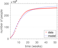
(a) Cumulative number

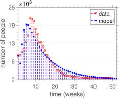
(b) New cases

Figure 6: Outbreak data (red) and calibrated model response (blue) from Table 2.

$\bm{\alpha}$	TRR input	$\mathbf{lb}$	$\mathbf{ub}$	TRR output	Reference
$\alpha_{h}$	$1/5.9$	$1/12$	$1/3$	$1/12$	[44, 45, 46, 15, 47, 40]
$\alpha_{v}$	$1/9.1$	$1/10$	$1/5$	$1/10$	[41, 43, 40]
$\gamma$	$1/7.9$	$1/8.8$	$1/3$	$1/3$	[47, 25, 40]
$\delta$	$1/11$	$1/21$	$1/11$	$1/21$	[51, 50, 47, 49]
$\beta_{h}$	$1/11.3$	$1/16.3$	$1/8$	$1/10.40$	[40]
$\beta_{v}$	$1/8.6$	$1/11.6$	$1/6.2$	$1/7.77$	[40]
$S_{h}^{i}$	$205{,}953{,}959$	$0.9\times N_{h}$	$N_{h}$	$205{,}953{,}534$	———–
$E_{h}^{i}$	$8{,}201$	$0$	$10{,}000$	$6{,}827$	———–
$I_{h}^{i}$	$8{,}201$	$0$	$10{,}000$	$10{,}000$	———–
$S_{v}^{i}$	$0.99956$	$0.99$	$0.999$	$0.999586$	———–
$E_{v}^{i}$	$2.2\times 10^{-4}$	$0$	$1$	$4.14\times 10^{-4}$	———–
$I_{v}^{i}$	$2.2\times 10^{-4}$	$0$	$1$	$0$	———–

Table 2: TRR setup for the Figure 6 calibrated response. The values referring to parameters are in $\text{days}^{-1}$, human IC are expressed in individuals, and vector quantities in proportion.

To compare the two systems defined by the parameters and IC from each table, Figure 7 portrays their $I_{h}$ response. The system from Table 1 has an almost monotonically decreasing $I_{h}$ curve, except for a slight local maximum around the $6$th EW, while the system from Table 2 presents a significant increase in the number of infectious individuals by the same time, which correspond to the weeks right before the peak infection. As stated, the lack of empirical data for the current number of infectious at each EW makes it impossible to determine what is a quantitatively reasonable prediction for $I_{h}$ values. But this work assumes that a more possible scenario involves a $I_{h}$ time series that also follows the general shape of an epidemic curve around the weeks of maximum infection, especially considering that Figure 7(a) implicates the notion that most people were infected strictly before $2016$, which does not seems the case suggested by the Brazilian outbreak data of probable cases of infected per EW [12] when compared to numbers available for $2015$ [13]. Thus, with this qualitative criteria in mind, the system from Table 2 is selected for a further analysis over its behavior dependency to the $I_{h}^{i}$ initial condition.

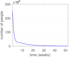
(a) $I_{h}(t)$ response from Table 1

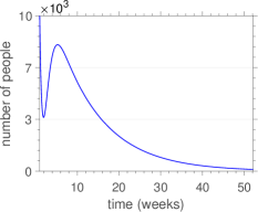
(b) $I_{h}(t)$ response from Table 2

Figure 7: Comparison between $I_{h}(t)$ responses from Table 1 (left) and Table 2 (rigth).

Figure 8 displays the $C(t)$, $\mathcal{N}_{w}$ and $I_{h}(t)$ responses per EW for various $I_{h}^{i}$ on the system with parameters from Table 2. To simplify the analysis, $E_{h}^{i}$ is considered equal to $I_{h}^{i}$ in each case. The remaining IC are the same from the Table. The pattern suggests that a $I_{h}^{i}$ increase on the system with this given set of parameters continuously escalates the $C(t)$ and $\mathcal{N}_{w}$ curves, eventually overshooting the data by far, and reduces the variations of $I_{h}(t)$ curve around its local maximum. Figure 8 allows one to make better predictions about the outbreak by analyzing the multiple possible scenarios of epidemic evolution over different values for the IC missing empirical information. Clearly, the system response in all cases is qualitative reliable in simulating the outbreak ($C(t)$ and $\mathcal{N}_{w}$ shape) and can quantitatively approximate the real data values for some values of $I_{h}^{i}$.

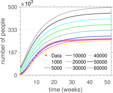
(a) Cumulative number

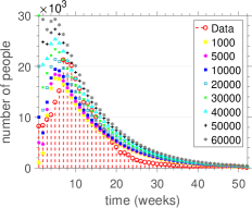
(b) New cases

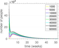
(c) $I_{h}$ response

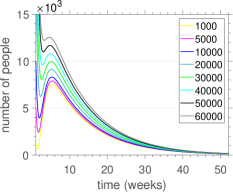
(d) $I_{h}$ response magnified

Figure 8: Multiple $C(t)$, $\mathcal{N}_{w}$ and $I_{h}(t)$ responses per EW using the parameters from Table 2. The values on the legend correspond to the used $I_{h}^{i}$ and $E_{h}^{i}$ to generate the curves. The other IC are also from Table 2. The bottom right graph is the $I_{h}$ comparison magnified around the local maximum region. The red circles are the previously used real data.

4 Concluding remarks

A SEIR-SEI epidemic model to describe the dynamics of the 2016 Zika virus outbreak in Brazl is developed and calibrated in this work. Nominal quantities for the parameters are selected from the related literature concerning the Zika infection, the Aedes aegypti genus of mosquitoes, vector-born epidemic models and information provided by health organizations. The calibration process is done through the solution of an inverse problem with the aid of a Trust-Region-Reflective method, used to pick the best parameter values that would fit the model response for the number of new infectious cases per week into the disease’s empirical data. Results within realistic values for the parameters are presented, stating reasonable descriptions with the curve shape similar to the outbreak evolution and proximity between the estimated peak value and data for maximum number of infected during 2016. Further analysis of the results about the lack of data for an initial condition is performed, exhibiting a range of values over which the system response keeps its quantitative reliability to a certain degree.

This work is part of a long project of modeling and prediction of epidemics related to the Zika virus in the Brazilian context [23, 24]. In upcoming studies the authors intend to take into account the uncertainties underlying the model parameters via Bayesian updating and employ an Active Subspace approach [59, 60, 61] to explore relevant scenarios in parametric studies.

References

References

- Brasil et al. [2016] P. Brasil et al. Zika virus outbreak in Rio de Janeiro, Brasil: clinical characterization, epidemiological and virological aspects. PLoS Negl. Trop. Dis., 10(4), 2016. doi: 10.1371/journal.pntd.0004636.
- Organization [2016] World Health Organization. Zika Virus. http://www.who.int/mediacentre/factsheets/zika/en/, 2016. Accessed: 08/18/2017.
- Fernandes et al. [2016] R. S. Fernandes et al. Culex quinquefasciatus from Rio de Janeiro is not competent to transmit the local Zika virus. PLoS Negl. Trop. Dis., 10(9), 2016. doi: 10.1371/journal.pntd.0004993.
- Petersen et al. [2016] E. E. Petersen et al. Update: Interim Guidance for Preconception Counseling and Prevention of Sexual Transmission of Zika Virus for Persons with Possible Zika Virus Exposure– United States, September 2016. MMWR Morb. Mortal. Wkly. Rep., 65(39):1077–1081, 2016. doi: 10.15585/mmwr.mm6539e1.
- Coelho et al. [2016] F. C. Coelho et al. Higher incidence of Zika in adult women than adult men in Rio de Janeiro suggests a significant contribution of sexual transmission from men to women. Int. J. Infect. Dis., 51:128–132, 2016. doi: 10.1016/j.ijid.2016.08.023.
- Motta et al. [2016] I. J. F. Motta, B. R. Spencer, et al. Evidence for Transmission of Zika Virus by Platelet Transfusion. N. Engl. J. Med., 375(11):1101–1103, 2016. doi: 10.1056/NEJMc1607262.
- Dick et al. [1952] G. W. A. Dick, S. F. Kitchen, and A. J. Haddow. Zika virus (I). Isolations and serological specificity. Trans. R. Soc. Trop. Med. Hyg., 46(5):509–520, 1952. doi: 10.1016/0035-9203(52)90042-4.
- Moore et al. [1975] D. L. Moore et al. Arthropod-borne viral infections of man in Nigeria, 1964–1970. Ann. Trop. Med. Parasitol., 69(1):49–64, 1975. doi: 10.1080/00034983.1975.11686983.
- Duffy et al. [2009] M. R. Duffy et al. Zika virus outbreak on Yap Island, Federated States of Micronesia. N. Engl. J. Med., 360(24):2536–2543, 2009. doi: 10.1056/NEJMoa0805715.
- Cao-Lormeau et al. [2014] V.-M. Cao-Lormeau et al. Zika virus, French Polynesia, South Pacific, 2013. Emerg. Infect. Dis., 20(6):1085–1086, 2014. doi: 10.3201/eid2006.140138.
- Tognarelli et al. [2016] J. Tognarelli et al. A report on the outbreak of Zika virus on Easter Island, South Pacific, 2014. Arch. Virol., 161(3):665–668, 2016. doi: 10.1007/s00705-015-2695-5.
-
Secretaria de Vigilância em Saúde [2017]
Secretaria de Vigilância em Saúde.
Boletim Epidemiolólico. monitoramento dos casos de dengue, febre
de chikungunya e febre pelo vírus Zika até a Semana
Epidemiológica 52, Volume 48.
http://portalarquivos.saude.gov.br/images/pdf/2017/abril/06/2017-002-Monitoramento-dos-casos-de-dengue--febre-de-chikungu
nya-e-febre-pelo-v--rus-Zika-ate-a-Semana-Epidemiologica-52
--2016.pdf, 2017. Accessed: 08/18/2017. - Faria et al. [2016] N. R. Faria, R. S. S. Azevedo, et al. Zika virus in the Americas: early epidemiological and genetic findings. Science, 352(6283):345–349, 2016. doi: 10.1126/science.aaf5036.
- Hennessey et al. [2016] M. Hennessey, M. Fischer, and J. E. Staples. Zika virus spreads to new areas — Region of the Americas, May 2015–January 2016. MMWR Morb. Mortal. Wkly. Rep., 65(3):55–58, 2016. doi: 10.15585/mmwr.mm6503e1.
- Valentine et al. [2016] G. Valentine, L. Marquez, and M. Pammi. Zika virus-associated microcephaly and eye lesions in the newborn. J. Pediatric. Infect. Dis. Soc., 5(3):323–328, 2016. doi: 10.1093/jpids/piw037.
- dos Santos et al. [2016] T. dos Santos et al. Zika virus and the Guillain–Barré syndrome — Case series from seven countries. N. Engl. J. Med., 375(16):1598–1601, 2016. doi: 10.1056/NEJMc1609015.
- World Health Organization [2016] World Health Organization. Zika virus, Microcephaly and Guillain-Barré Syndrome - Situation Report. http://www.who.int/emergencies/zika-virus/situation-report/7-april-2016/en/, 2016. Accessed: 08/18/2017.
- Naheed and M. Singh [2014] A. Naheed and D. Lucy M. Singh. Numerical study of SARS epidemic model with the inclusion of diffusion in the system. Appl. Math. Comput., 229:480–498, 2014. doi: 10.1016/j.amc.2013.12.062.
- Huppert and Katriel [2013] A. Huppert and G. Katriel. Mathematical modelling and prediction in infectious disease epidemiology. Clin. Microbiol. Infect., 19:999–1005, 2013. doi: 10.1111/1469-0691.12308.
- Lizarralde-Bejarano et al. [2017] D. P. Lizarralde-Bejarano, S. Arboleda-Sánchez, and M. E. Puerta-Yepes. Understanding epidemics from mathematical models: Details of the 2010 dengue epidemic in Bello (Antioquia, Colombia). Appl. Math. Model., 43:566–578, 2017. doi: 10.1016/j.apm.2016.11.022.
- Oberkampf and Roy [2010] W. L. Oberkampf and C. J. Roy. Verification and Validation in Scientific Computing. Cambridge University Press, 2010. ISBN 978-0-521-11360-1.
- Cunha Jr [2017] A. Cunha Jr. Modeling and Quantification of Physical Systems Uncertainties in a Probabilistic Framework. In S. Ekwaro-Osire, A. C. Gonçalves, and F. M. Alemayehu, editors, Probabilistic Prognostics and Health Management of Energy Systems, pages 127–156. Springer International Publishing, New York, 2017. doi: 10.1007/978-3-319-55852-3_8.
- E. Dantas, M. Tosin, J. Peterson, V. Lopes, A. Cunha Jr [2016] E. Dantas, M. Tosin, J. Peterson, V. Lopes, A. Cunha Jr. A mathematical analysis about Zika virus outbreak in Rio de Janeiro. In 4th Conference of Computational Interdisciplinary Science (CCIS 2016), São José dos Campos, Brazil, 2016.
- E. Dantas, M. Tosin, A. Cunha Jr [in press] E. Dantas, M. Tosin, A. Cunha Jr. Zika virus in Brazil: calibration of an epidemic model for 2016 outbreak. In XXXVII Congresso Nacional de Matemática Aplicada e Computacional (CNMAC 2017), São José dos Campos, Brazil, in press.
- Funk et al. [2016] S. Funk et al. Comparative analysis of Dengue and Zika outbreaks reveals differences by setting and virus. PLoS Negl. Trop. Dis., 10(12), 2016. doi: 10.1371/journal.pntd.0005173.
- Kucharski et al. [2016] A. J. Kucharski, S. Funk, R. M. Eggo, H. P. Mallet, W. J Edmunds, and E. J. Nilles. Transmission dynamics of Zika virus in island populations: a modelling analysis of the 2013–14 French Polynesia outbreak. PLoS Negl. Trop. Dis., 10(5), 2016. doi: 10.1371/journal.pntd.0004726.
- Wang et al. [2014] X. Wang, L. Wei, and J. Zhang. Dynamical analysis and perturbation solution of an SEIR epidemic model. Appl. Math. Comput., 232:479–486, 2014. doi: 10.1016/j.amc.2014.01.090.
- Wanga et al. [2017] Y. Wanga, J. Cao, A. Alsaedi, and B. Ahmade. Edge-based SEIR dynamics with or without infectious force in latent period on random networks. Commun. Nonlinear Sci. Numer. Simul., 45:35–54, 2017. doi: 10.1016/j.cnsns.2016.09.014.
- Safi et al. [2013] M. A. Safi, A. B. Gumel, and E. H. Elbasha. Qualitative analysis of an age-structured SEIR epidemic model with treatment. Appl. Math. Comput., 219(22):10627–10642, 2013. doi: 10.1016/j.amc.2013.03.126.
- Cai et al. [2017] Y. Cai, Y. Kang, and W. Wang. A stochastic SIRS epidemic model with nonlinear incidence rate. Appl. Math. Comput., 305:221–240, 2017. doi: 10.1016/j.amc.2017.02.003.
- Smith et al. [2012] D. L. Smith, K. E. Battle, S. I. Hay, C. M. Barker, T. W. Scott, F. E. McKenzie, et al. Ross, MacDonald, and a theory for the dynamics and control of mosquito - Transmitted pathogens. PLoS Pathog., 8(4), 2012. doi: 10.1371/journal.ppat.1002588.
- F. Brauer, C. Castillo-Chavez [2012] F. Brauer, C. Castillo-Chavez, editor. Mathematical Models in Population Biology and Epidemiology. Springer, second edition, 2012. doi: 10.1007/978-1-4614-1686-9.
- Brauer et al. [2008] F. Brauer, P. van den Driessche, and J. Wu, editors. Mathematical Epidemiology. Springer, 2008. doi: 10.1007/978-3-540-78911-6.
- Martcheva [2015] M. Martcheva. An Introduction to Mathematical Epidemiology. Springer, first edition, 2015. doi: 10.1007/978-1-4899-7612-3_1.
- Chan and Johansson [2012] M. Chan and M. A. Johansson. The incubation periods of Dengue viruses. PLoS ONE, 7(11), 2012. doi: 10.1371/journal.pone.0050972.
- Lessler et al. [2016] J. Lessler, L. H. Chaisson, et al. Assessing the global threat from Zika virus. Science, 353(6300), 2016. doi: 10.1126/science.aaf8160.
- Begon et al. [2002] M. Begon, M. Bennett, R. G. Bowers, et al. A clarification of transmission terms in host-microparasite models: numbers, densities and areas. Epidemiol. Infect., 129, 2002. doi: 10.1017/S0950268802007148.
- Ministeŕio da Saúde [2017] Ministeŕio da Saúde. Obtenção de número de casos confirmados de zika, por municiṕio e semana epidemioloǵica. http://www.consultaesic.cgu.gov.br/busca/dados/Lists/Pedido/Item/displayifs.aspx?List=0c839f31-47d7-4485-ab65-ab0cee9cf8fe&ID=537263&Web=88cc5f44-8cfe-4964-8ff4-376b5ebb3bef, 2017. Accessed: 08/18/2017.
- Fundação Instituto Brasileiro de Geografia e Estatística [2016] Fundação Instituto Brasileiro de Geografia e Estatística. Diário Oficial da União, N. 167- Seção 1. Imprensa Nacional, 2016. p. 47–65. Brasília.
- Ferguson et al. [2016] N. M. Ferguson, , et al. Countering the Zika epidemic in Latin America. Science, 353(6297):353–354, 2016. doi: 10.1126/science.aag0219.
- P.-S. J. Wong, M. I. Li, C.-S. Chong, L.-C. Ng, C.-H. Tan [2013] P.-S. J. Wong, M. I. Li, C.-S. Chong, L.-C. Ng, C.-H. Tan. Aedes (Stegomyia) albopictus (Skuse): A Potential Vector of Zika Virus in Singapore. PLoS Negl. Trop. Dis., 7(8), 2013. doi: 10.1371/journal.pntd.0002348.
- M. I. Li, P.-S. J. Wong, L.-C. Ng, C.-H. Tan [2012] M. I. Li, P.-S. J. Wong, L.-C. Ng, C.-H. Tan. Oral Susceptibility of Singapore Aedes (Stegomyia) aegypti (Linnaeus) to Zika Virus. PLoS Negl. Trop. Dis., 6(8), 2012. doi: 10.1371/journal.pntd.0001792.
- Chouin-Carneiro et al. [2016] T. Chouin-Carneiro, A. Vega-Rua, et al. Differential Susceptibilities of Aedes aegypti and Aedes albopictus from the Americas to Zika Virus. PLoS Negl. Trop. Dis., 10(3), 2016. doi: 10.1371/journal.pntd.0004543.
- Ott et al. [2016] C. T. Ott, J. T. Lessler, et al. Times to key events in Zika virus infection and implications for blood donation: a systematic review. Bull. World Health Organ., 94:841–849, 2016. doi: 10.2471/BLT.16.174540.
- Ioos et al. [2014] S. Ioos, H.-P. Mallet, I. L. Goffart, V. Gauthier, T. Cardoso, and M. Herida. Current Zika virus epidemiology and recent epidemics. Med. Mal. Infect., 44(7):302–307, 2014. doi: 10.1016/j.medmal.2014.04.008.
- European Centre for Disease Prevention and Control [2015] European Centre for Disease Prevention and Control. Rapid risk assessment: Microcephaly in Brazil potentially linked to the Zika virus epidemic. https://ecdc.europa.eu/sites/portal/files/media/en/publications/Publications/zika-\microcephaly-Brazil-rapid-risk-assessment-Nov-2015.pdf, 2015. Accessed: 08/18/2017.
- Villela et al. [2017] D. A. M. Villela, L. S. Bastos, et al. Zika in Rio de Janeiro: Assessment of basic reproduction number and comparison with dengue outbreaks. Epidemiol. Infect., 145(8):1649–1657, 2017. doi: 10.1017/S0950268817000358.
- Otero et al. [2006] M. Otero, H. G. Solari, and N. Schweigmann. A stochastic population dynamics model for Aedes Aegypti: formulation and application to a city with temperate climate. Bull. Math. Biol., 68(8):1945–1974, 2006. doi: 10.1007/s11538-006-9067-y.
- R. M. de Freitas [2007] R. L. de Oliveira R. M. de Freitas, C. T. Codeço. Daily survival rates and dispersal of Aedes aegypti females in Rio de Janeiro, Brazil. Am. J. Trop. Med. Hyg., 76(4):659–665, 2007.
- Nelson [1986] M. J. Nelson. Aedes Aegypti: Biology and Ecology. Pan American Health Organization, Washington, D.C., 1986.
- National Center for Emerging and Zoonotic Infectious Diseases [2012] National Center for Emerging and Zoonotic Infectious Diseases. Dengue and the Aedes aegypti mosquito. https://www.cdc.gov/dengue/resources/30jan2012/aegyptifactsheet.pdf, 2012. Accessed: 08/18/2017).
- Hirsch et al. [2013] M. W Hirsch, S. Smale, and R. L. Devaney. Differential Equations, Dynamical Systems, and an Introduction to Chaos. Academic Press, 3rd edition, 2013.
- Perko [2006] L. Perko. Differential Equations and Dynamical Systems. Springer, 3rd edition, 2006.
- Aster et al. [2012] R. Aster, B. Borchers, and C. Thurber, editors. Parameter Estimation and Inverse Problems. Elsevier, second edition, 2012. ISBN 978-0-128-10092-9.
- Yaman et al. [2013] F. Yaman, V. G. Yakhno, and R. Potthast. A Survey on Inverse Problems for Applied Sciences. Math. Probl. Eng., 2013, 2013. doi: 10.1155/2013/976837.
- Chavent. [2010] G. Chavent. Nonlinear Least Squares for Inverse Problems: Theoretical Foundations and Step-by-Step Guide for Applications. Springer, 2010. doi: 10.1007/978-90-481-2785-6.
- Coleman and Li. [1996] T. F. Coleman and Y. Li. An interior, trust region approach for nonlinear minimization subject to bounds. SIAM J. Optim., 6(2):418–445, 1996. doi: 10.1137/0806023.
- Conn et al. [2000] A. R. Conn, N. I.M. Gould, and P. L. Toint, editors. Trust Region Methods. SIAM, 2000.
- Constantine [2015] P. G. Constantine. Active Subspaces: Emerging Ideas for Dimension Reduction in Parameter Studies. SIAM, 2015. doi: 10.1137/1.9781611973860.
- Diaz et al. [2018] P. Diaz, P. Constantine, K. Kalmbach, E. Jones, and S. Pankavich. A modified SEIR model for the spread of Ebola in Western Africa and metrics for resource allocation. Appl. Math. Comput., 324:141–155, 2018. doi: 10.1137/130916138.
- Constantine et al. [2014] P. G. Constantine, E. Dow, and Q. Wang. Active Subspace Methods in Theory and Practice: Applications to Kriging Surfaces. SIAM J. Sci. Comput., 36(4):1500–1524, 2014. doi: 10.1137/130916138.