GIPA: General Information Propagation Algorithm for Graph Learning

Abstract.

Graph neural networks (GNNs) have been popularly used in analyzing graph-structured data, showing promising results in various applications such as node classification, link prediction and network recommendation. In this paper, we present a new graph attention neural network, namely GIPA, for attributed graph data learning. GIPA consists of three key components: attention, feature propagation and aggregation. Specifically, the attention component introduces a new multi-layer perceptron based multi-head to generate better non-linear feature mapping and representation than conventional implementations such as dot-product. The propagation component considers not only node features but also edge features, which differs from existing GNNs that merely consider node features. The aggregation component uses a residual connection to generate the final embedding. We evaluate the performance of GIPA using the Open Graph Benchmark proteins (ogbn-proteins for short) dataset. The experimental results reveal that GIPA can beat the state-of-the-art models in terms of prediction accuracy, e.g., GIPA achieves an average test ROC-AUC of $0.8700\pm 0.0010$ and outperforms all the previous methods listed in the ogbn-proteins leaderboard.

1. Introduction

Graph representation learning typically aims to learn an informative embedding for each graph node based on the graph topology (link) information. Generally, the embedding of a node is represented as a low-dimensional feature vector, which can be used to facilitate downstream applications. This research starts from homogeneous graphs that have only one type of nodes and one type of edges. The purpose is to learn node representations from the graph topology (Grover and Leskovec, 2016; Perozzi et al., 2014; Dai et al., 2016). Specifically, given a node $u$, either breadth-first search, depth-first search or random walks is used to identify a set of neighboring nodes. Then, the $u$’s embedding is learnt by maximizing the co-occurrence probability of $u$ and its neighbors. In reality, nodes and edges can carry a rich set of information such as attributes, texts, images or videos, beyond graph structure. These information can be used to generate node or edge feature by means of a feature transformation function, which further improves the performance of network embedding (Liao et al., 2018).

These pioneer studies on graph embedding have limited capability to capturing neighboring information from a graph because they are based on shallow learning models such as SkipGram (Mikolov et al., 2013). Moreover, transductive learning is used in these graph embedding methods which cannot generalize to new nodes that are absent in the training graph.

On the other hand, graph neural networks (Kipf and Welling, 2016; Hamilton et al., 2017; Veličković et al., 2018) are proposed to overcome the limitations of graph embedding models. GNNs employ deep neural networks to aggregate feature information from neighboring nodes and thereby have the potential to gain better aggregated embedding. GNNs can support inductive learning and infer the class labels of unseen nodes during prediction (Hamilton et al., 2017; Veličković et al., 2018). The success of GNNs is mainly based on the neighborhood information aggregation. Two critical challenges to GNNs are which neighboring nodes of a target node are involved in message passing, and how much contribution each neighboring node makes to the aggregated embedding. For the former question, neighborhood sampling (Hamilton et al., 2017; Ying et al., 2018; Chen et al., 2018; Huang et al., 2018; Zou et al., 2019; Ji et al., 2020) is proposed for large dense or power-law graphs. For the latter, neighbor importance estimation is used to add different weights to different neighboring nodes during feature propagation. Importance sampling (Chen et al., 2018; Zou et al., 2019; Ji et al., 2020) and attention (Veličković et al., 2018; Liu et al., 2019; Wang et al., 2019a; Yun et al., 2019; Hu et al., 2020a) are two popular techniques.

Importance sampling is a specialization of neighborhood sampling, where the importance weight of a neighboring node is drawn from a distribution over nodes. This distribution can be derived from normalized Laplacian matrices (Chen et al., 2018; Zou et al., 2019) or jointly learned with GNNs (Ji et al., 2020). With this distribution, each step samples a subset of neighbors and aggregates their information with importance weights. Similar to importance sampling, attention also adds importance weights to neighbors. Nevertheless, attention differs from importance sampling. Attention is represented as a neural network and always learned as a part of a GNN model. In contrast, importance sampling algorithms use statistical models without trainable parameters. Existing attention ranks nodes but does not drop off any of them. On the contrary, importance sampling reduces the number of neighbors. Basically, we would expect an (almost equal to) zero importance score for noise neighbors and higher scores for strongly correlated neighbors.

In this paper, we present a new graph attention neural network, namely GIPA (General Information Propagation Algorithm), for attributed graphs. In general, GIPA consists of three components, i.e., attention, propagation and aggregation. The attention component uses a multi-head method which is implemented with a multi-layer perceptron (MLP). The propagation component incorporates both node and edge features, unlike GAT (Veličković et al., 2018) that uses only node features. The aggregation component reduces messages from the neighbors of a given node $i$ and concatenates the resulted message with a linear projection of node $i$’s features by means of a residual connection. Experiments on the Open Graph Benchmark (OGB) (Hu et al., 2020b) proteins dataset (ogbn-proteins) demonstrate that GIPA reaches the best accuracy with an average test ROC-AUC of $0.8700\pm 0.0010$ compared with the state-of-the-art methods listed in the ogbs-proteins leaderboard . Up to date, this performance has been exhibited to the public in the leaderboard with GIPA in the first place, as shown in Figure 1.

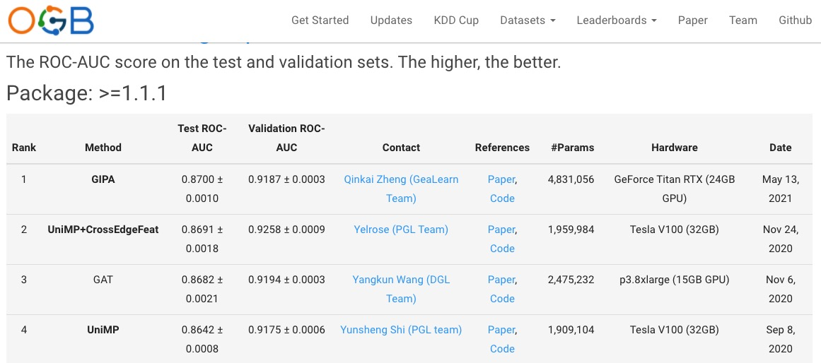
Figure 1. A snapshot of the leaderboard of ogbn-proteins with GIPA as the champion.

2. Related Work

In this part, we survey existing attention primitive implementations in brief. (Bahdanau et al., 2015) proposed an additive attention that calculates the attention alignment score using a simple feed-forward neural network with only one hidden layer. The alignment score $score(q,k)$ between two vectors $q$ and $k$ is defined as

(1) $$score(q,k)=u^{T}\tanh(W[q;k]),$$

where $u$ is an attention vector and the attention weight $\alpha_{q,k}$ is computed by normalizing $score_{q,k}$ over all ${q,k}$ values with the softmax function. The core of the additive attention lies in the use of attention vector $u$. This idea has been widely adopted by several algorithms (Yang et al., 2016; Pavlopoulos et al., 2017) for neural language processing. (Luong et al., 2015) introduces a global attention and a local attention. In global attention, the alignment score can be computed by three alternatives: dot-product ($q^{T}k$), general ($q^{T}Wk$) and concat ($W[q;k]$). In contrast, local attention computes the alignment score solely from a vector ($Wq$). Likewise, both global and local attention normalize the alignment scores with the softmax function. (Vaswani et al., 2017) proposed a self-attention mechanism based on scaled dot-products. This self-attention computes the alignment scores between any $q$ and $k$ as follows.

(2) $$score_{q,k}=\frac{q^{T}k}{\sqrt{d_{k}}}$$

This attention differs from the dot-product attention (Luong et al., 2015) by only a scaling factor of $\frac{1}{\sqrt{d_{k}}}$. The scaling factor is used because the authors of (Vaswani et al., 2017) suspected that for large values of $d_{k}$, the dot-products grow large in magnitude and thereby push the softmax function into regions where it has extremely small gradients. Furthermore, a multi-head mechanism is proposed in order to stabilize the self-attention values computed.

In this paper, we introduce an MLP based multi-head implementation to compute attention scores. In addition, these aforementioned attention primitives have been extended to use in heterogeneous graph models. HAN (Wang et al., 2019a) uses a two-level hierarchical attention made out of a node-level attention and a semantic-level attention. In HAN, the node-level attention learns the importance of a node to any other node in a meta-path, while the semantic-level one weighs all meta-paths. HGT (Zhang et al., 2019) weakens the dependency on meta-paths and instead uses meta-relation triplets as basic units. In HGT, it uses node-type-aware feature transform functions and edge-type-aware multi-head attention to compute the importance of each edge to a target node. It needs to be addressed that no evidence shows that heterogeneous models are always superior to homogeneous ones, and vice versa.

3. Methodology

3.1. Preliminaries

Graph Neural Networks.

Consider an attributed graph $\mathcal{G}=\{\mathcal{V},\mathcal{E}\}$, where $\mathcal{V}$ is the set of nodes and $\mathcal{E}$ is the set of edges. GNNs use the same model framework as follows (Hamilton et al., 2017; Xu et al., 2018):

(3) $$h_{i}^{k}=\phi(h_{i}^{k-1},\mathcal{F}_{agg}(\{h_{j},j\in\mathcal{N}(i)\}))$$

where $\mathcal{F}_{agg}$ represents an aggregation function and $\phi$ represents an update function. The objective of GNNs is to update the embedding of each node by aggregating the information from its neighbor nodes and the connections between them.

3.2. GIPA Architecture

In this part, we present the architecture of GIPA, which extracts information from node features as well as edge features in a more general way. The process of GIPA is shown in Figure 2. Consider a node $i$ with feature $h_{i}$ and its neighbor nodes $j\in\mathcal{N}(i)$ with feature $h_{j}$. $e_{i,j}$ represents the edge feature between node $i$ and $j$. The problem is how to generate an expected embedding for node $i$ from its own node feature $h_{i}$, its neighbors’ node features $\{h_{j}\}$ and the related edge features $\{e_{i,j}\}$.

The GIPA process mainly consists of three parts: attention, propagation and aggregation. Firstly, GIPA computes the embedding $\tilde{h}_{i}$, $\tilde{h}_{j}$, and $\tilde{e}_{i,j}$ by means of linear projection from the features $h_{i}$, $h_{j}$ and $e_{i,j}$, respectively. Secondly, the attention process calculates the multi-head attention weights by using fully-connected layers on $\tilde{h}_{i}$, $\tilde{h}_{j}$, and $\tilde{e}_{i,j}$, respectively. Thirdly, the propagation process focuses on propagating information of each neighbor node $j$ by combining $j$’s node embedding $\tilde{h}_{j}$ with the associated edge embedding $\tilde{e}_{i,j}$. Finally, the aggregation process aggregates all messages from neighbors to update the embedding of $i$. The following subsections introduce the details of each process.

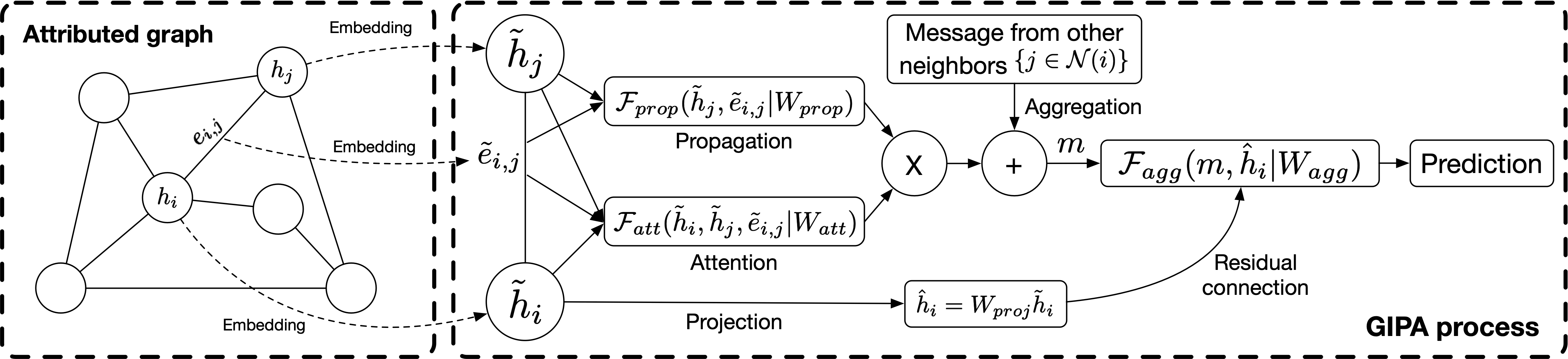
Figure 2. Process of GIPA, which consists of attention, propagation, and aggregation process.

3.2.1. Attention Process

Different from the existing attention mechanisms like self-attention or scaled dot-product attention, we use MLP to realize a multi-head attention mechanism. The attention process of GIPA can be formulated as follows:

(4) $$\tilde{a}_{i,j}=\mathcal{F}_{att}(\tilde{h}_{i},\tilde{h}_{j},\tilde{e}_{i,j}|W_{att})=\text{MLP}([\tilde{h}_{i}||\tilde{h}_{j}||\tilde{e}_{i,j}]|W_{att})$$

where the attention function $\mathcal{F}_{att}$ is realized by an MLP with learnable weights $W_{att}$ (without bias). Its input is the concatenation of the node embedding $\tilde{h}_{i}$ and $\tilde{h}_{j}$ as well as the edge embedding $\tilde{e}_{i,j}$. As the scale of parameters of MLP is adjustable, this attention mechanism could be more representative than previous ones simply based on dot-product. The final attention weight is calculated by an edge-wise softmax activation function:

(5) $$a_{i,j}=\text{softmax}(\tilde{a}_{i,j})=\frac{\exp(\tilde{a}_{i,j})}{\sum_{k\in N(i)}\exp(\tilde{a}_{i,k})}$$

3.2.2. Propagation Process

Unlike GAT (Veličković et al., 2018) that only considers the node feature of neighbors, GIPA incorporates both node and edge features during the propagation process:

(6) $$p_{i,j}=\mathcal{F}_{prop}(\tilde{h}_{j},\tilde{e}_{i,j}|W_{prop})=\text{MLP}([\tilde{h}_{j}||\tilde{e}_{i,j}]|W_{prop}),$$

where the propagation function $\mathcal{F}_{prop}$ is also realized by an MLP with learnable weights $W_{prop}$. Its input is the concatenation of a neighbor node embedding $\tilde{h}_{j}$ and the related edge embedding $\tilde{e}_{i,j}$. Thus, the $propagation$ is done edge-wise rather than node-wise.

Combining the results by attention and propagation by element-wise multiplication, GIPA gets the message $m_{i,j}$ of node $i$ from $j$:

(7) $$m_{i,j}=a_{i,j}*p_{i,j}$$

3.2.3. Aggregation Process

For each node $i$, GIPA repeats previous processes to get messages from its neighbors. The aggregation process first gathers all these messages by a reduce function, summation for example:

(8) $$m_{i}=\sum_{j\in\mathcal{N}(i)}m_{i,j}$$

Then, a residual connection between the linear projection $\hat{h}_{i}$ and the message of $m_{i}$ is added through concatenation:

(9) $$\hat{h}_{i}=W_{proj}\tilde{h}_{i}$$

(10) $$o_{i}=\mathcal{F}_{agg}(m,\hat{h}_{i}|W_{agg})=\text{MLP}([\sum_{j\in\mathcal{N}(i)}m_{i,j}||\hat{h}_{i}]|W_{agg})$$

where an MLP with learnable weights $W_{agg}$ is applied to get the final output $o_{i}$. Finally, we would like to emphasize that the process of GIPA can be easily extended to multi-layer variants by stacking the process multiple times.

4. Experiments

4.1. Dataset and Settings

Dataset. In our experiments, the ogbn-proteins dataset from OGB (Hu et al., 2020b) is used. The dataset is an undirected and weighted graph, containing 132,534 nodes of 8 different species and 79,122,504 edges with 8-dimensional features. The task is a multi-label binary classification problem with 112 classes representing different protein functions.

Evaluation metric. The performance is measured by the average ROC-AUC scores. We follow the dataset splitting settings as recommended in OGB and test the performance of 10 different trained models with different random seeds.

Hyperparameters. The hyperparamters used in GIPA and its training process are concluded in Table 1.

Environment. GIPA is implemented in Deep Graph Library (DGL) (Wang et al., 2019b) with Pytorch (Paszke et al., 2019) as the backend. The experiments are done in a platform with GeForce TITAN RTX GPU (24GB RAM) and AMD Ryzen Threadripper 3960X CPU (24 Cores).

Table 1. Hyperparameters of GIPA model.

Hyperparameter	Value
Node embedding length	80
Edge embedding length	16
Number of attention layers	2
Number of attention heads	8
Number of propagation layers	2
Number of hidden units	80
Number of GIPA layers	6
Edge drop rate	0.1
Aggregation	SUM
Activation	ReLU
Dropout of node embedding	0.1
Dropout of attention	0.1
Dropout of propagation	0.25
Dropout of aggregation	0.25
Dropout of the last FC layer	0.5
Learning rate	0.01
Optimizer	AdamW (Loshchilov and Hutter, 2019)

Table 2. Test and validation performance (ROC-AUC) on ogbn-proteins dataset.

Method	Test ROC-AUC	Validation ROC-AUC
MLP	$0.7204\pm 0.0048$	$0.7706\pm 0.0014$
GCN	$0.7251\pm 0.0035$	$0.7921\pm 0.0018$
GraphSAGE	$0.7768\pm 0.0020$	$0.8334\pm 0.0013$
DeeperGCN	$0.8496\pm 0.0028$	$0.8971\pm 0.0011$
GAT	$0.8682\pm 0.0018$	$0.9194\pm 0.0003$
UniMP	$0.8642\pm 0.0008$	$0.9175\pm 0.0006$
UniMP+CrossEdgeFeat	$0.8691\pm 0.0018$	$\mathbf{0.9258\pm 0.0009}$
GIPA (ours)	$\mathbf{0.8700\pm 0.0010}$	$0.9187\pm 0.0003$

4.2. Performance

Table LABEL:tab:performance shows the average ROC-AUC and the standard deviation for the test set and the validation set, respectively. The results of the baselines are retrieved from the ogbn-proteins leaderboard. Our GIPA outperforms all previous methods in the leaderboard and reaches an average test ROC-AUC higher than 0.8700 for the first time.

5. Conclusion

We have presented GIPA, a new graph attention network architecture for attributed graph data learning. GIPA has investigated three technical novelties: an MLP based multi-head attention, a propagation function involving both node feature and edge feature, and a residual connection aggregation method. The performance evaluations on the ogbn-proteins dataset have demonstrated that GIPA yields an average test ROC-AUC of $0.8700\pm 0.0010$, showing the best results compared with the state-of-the-art methods listed in the ogbn-proteins leaderboard. In the future, we will extend GIPA to heterogeneous GNNs and conduct testing on the open graph datasets.

- (1)
- Bahdanau et al. (2015) Dzmitry Bahdanau, Kyunghyun Cho, and Yoshua Bengio. 2015. Neural machine translation by jointly learning to align and translate. In ICLR’15.
- Chen et al. (2018) Jie Chen, Tengfei Ma, and Cao Xiao. 2018. Fastgcn: fast learning with graph convolutional networks via importance sampling. In Proceedings of the 6th International Conference on Learning Representations.
- Dai et al. (2016) Hanjun Dai, Bo Dai, and Le Song. 2016. Discriminative embeddings of latent variable models for structured data. In International conference on machine learning. 2702–2711.
- Grover and Leskovec (2016) Aditya Grover and Jure Leskovec. 2016. node2vec: Scalable feature learning for networks. In Proceedings of the 22nd ACM SIGKDD international conference on Knowledge discovery and data mining. 855–864.
- Hamilton et al. (2017) Will Hamilton, Zhitao Ying, and Jure Leskovec. 2017. Inductive representation learning on large graphs. In NeurIPS’17. 1024–1034.
- Hu et al. (2020b) Weihua Hu, Matthias Fey, Marinka Zitnik, Yuxiao Dong, Hongyu Ren, Bowen Liu, Michele Catasta, and Jure Leskovec. 2020b. Open graph benchmark: Datasets for machine learning on graphs. In Advances in Neural Information Processing Systems.
- Hu et al. (2020a) Ziniu Hu, Yuxiao Dong, Kuansan Wang, and Yizhou Sun. 2020a. Heterogeneous graph transformer. In Proceedings of The Web Conference 2020. 2704–2710.
- Huang et al. (2018) Wenbing Huang, Tong Zhang, Yu Rong, and Junzhou Huang. 2018. Adaptive sampling towards fast graph representation learning. In Advances in neural information processing systems, Vol. 31. 4558–4567.
- Ji et al. (2020) Yugang Ji, Mingyang Yin, Hongxia Yang, Jingren Zhou, Vincent W Zheng, Chuan Shi, and Yuan Fang. 2020. Accelerating Large-Scale Heterogeneous Interaction Graph Embedding Learning via Importance Sampling. ACM Transactions on Knowledge Discovery from Data (TKDD) 15, 1 (2020), 1–23.
- Kipf and Welling (2016) Thomas N Kipf and Max Welling. 2016. Semi-supervised classification with graph convolutional networks. In International Conference on Learning Representations.
- Liao et al. (2018) Lizi Liao, Xiangnan He, Hanwang Zhang, and Tat-Seng Chua. 2018. Attributed social network embedding. IEEE Transactions on Knowledge and Data Engineering 30, 12 (2018), 2257–2270.
- Liu et al. (2019) Ziqi Liu, Chaochao Chen, Longfei Li, Jun Zhou, Xiaolong Li, Le Song, and Yuan Qi. 2019. Geniepath: Graph neural networks with adaptive receptive paths. In Proceedings of the AAAI Conference on Artificial Intelligence, Vol. 33. 4424–4431.
- Loshchilov and Hutter (2019) Ilya Loshchilov and Frank Hutter. 2019. Decoupled weight decay regularization. In ICLR’19.
- Luong et al. (2015) Minh-Thang Luong, Hieu Pham, and Christopher D Manning. 2015. Effective approaches to attention-based neural machine translation. In Proceedings of the 2015 conference on empirical methods in natural language processing. 1412–1421.
- Mikolov et al. (2013) Tomas Mikolov, Ilya Sutskever, Kai Chen, Greg S Corrado, and Jeff Dean. 2013. Distributed representations of words and phrases and their compositionality. In Advances in neural information processing systems, Vol. 26. 3111–3119.
- Paszke et al. (2019) Adam Paszke, Sam Gross, Francisco Massa, Adam Lerer, James Bradbury, Gregory Chanan, Trevor Killeen, Zeming Lin, Natalia Gimelshein, Luca Antiga, et al. 2019. Pytorch: An imperative style, high-performance deep learning library. In Advances in Neural Information Processing Systems.
- Pavlopoulos et al. (2017) John Pavlopoulos, Prodromos Malakasiotis, and Ion Androutsopoulos. 2017. Deeper attention to abusive user content moderation. In Proceedings of the 2017 conference on empirical methods in natural language processing. 1125–1135.
- Perozzi et al. (2014) Bryan Perozzi, Rami Al-Rfou, and Steven Skiena. 2014. Deepwalk: Online learning of social representations. In Proceedings of the 20th ACM SIGKDD international conference on Knowledge discovery and data mining. 701–710.
- Vaswani et al. (2017) Ashish Vaswani, Noam Shazeer, Niki Parmar, Jakob Uszkoreit, Llion Jones, Aidan N Gomez, Lukasz Kaiser, and Illia Polosukhin. 2017. Attention is all you need. In Advances in Neural Information Processing Systems.
- Veličković et al. (2018) Petar Veličković, Guillem Cucurull, Arantxa Casanova, Adriana Romero, Pietro Lio, and Yoshua Bengio. 2018. Graph attention networks. In ICLR’18.
- Wang et al. (2019b) Minjie Wang, Lingfan Yu, Da Zheng, Quan Gan, Yu Gai, Zihao Ye, Mufei Li, Jinjing Zhou, Qi Huang, Chao Ma, et al. 2019b. Deep Graph Library: Towards Efficient and Scalable Deep Learning on Graphs. In ICLR’19.
- Wang et al. (2019a) Xiao Wang, Houye Ji, Chuan Shi, Bai Wang, Yanfang Ye, Peng Cui, and Philip S Yu. 2019a. Heterogeneous graph attention network. In The World Wide Web Conference. 2022–2032.
- Xu et al. (2018) Keyulu Xu, Weihua Hu, Jure Leskovec, and Stefanie Jegelka. 2018. How Powerful are Graph Neural Networks?. In ICLR’18.
- Yang et al. (2016) Zichao Yang, Diyi Yang, Chris Dyer, Xiaodong He, Alex Smola, and Eduard Hovy. 2016. Hierarchical attention networks for document classification. In Proceedings of the 2016 conference of the North American chapter of the association for computational linguistics: human language technologies. 1480–1489.
- Ying et al. (2018) Rex Ying, Ruining He, Kaifeng Chen, Pong Eksombatchai, William L Hamilton, and Jure Leskovec. 2018. Graph convolutional neural networks for web-scale recommender systems. In Proceedings of the 24th ACM SIGKDD International Conference on Knowledge Discovery & Data Mining. 974–983.
- Yun et al. (2019) Seongjun Yun, Minbyul Jeong, Raehyun Kim, Jaewoo Kang, and Hyunwoo J Kim. 2019. Graph transformer networks. In Advances in Neural Information Processing Systems. 11983–11993.
- Zhang et al. (2019) Chuxu Zhang, Dongjin Song, Chao Huang, Ananthram Swami, and Nitesh V Chawla. 2019. Heterogeneous graph neural network. In Proceedings of the 25th ACM SIGKDD International Conference on Knowledge Discovery & Data Mining. 793–803.
- Zou et al. (2019) Difan Zou, Ziniu Hu, Yewen Wang, Song Jiang, Yizhou Sun, and Quanquan Gu. 2019. Layer-dependent importance sampling for training deep and large graph convolutional networks. In Advances in Neural Information Processing Systems. 11249–11259.