Heisenberg-Limited Waveform Estimation with Solid-State Spins in Diamond

Abstract

The newly established Heisenberg limit in arbitrary waveform estimation is quite different with parameter estimation and shows a unique characteristic of a future quantum version of oscilloscope. However, it is still a non-trivial challenge to generate a large number of exotic quantum entangled states to achieve this quantum limit. Here, by employing the time-domain quantum difference detection method, we demonstrate Heisenberg-limited waveform quantum estimation with diamond spins under ambient condition in the experiment. Periodic dynamical decoupling is applied to enhance both the dynamic range and sensitivity by one order of magnitude. Using this quantum-enhanced estimation scheme, the estimation error of an unknown waveform is reduced by more than $5$ dB below the standard quantum limit with $N\sim{\text{2}}\times{\text{1}}{{\text{0}}^{3}}$ resources, where more than ${1\times{\text{1}}{{\text{0}}^{5}}}$ resources would be required to achieve a similar error level using classical detection. This work provides an essential step towards realizing quantum-enhanced structure recognition in a continuous space and time.

Quantum metrology Giovannetti et al. (2011); Pezzè et al. (2018); Braun et al. (2018); Pirandola et al. (2018); Sun et al. (2008); Higgins et al. (2007); Dong et al. (2016); Kessler et al. (2014) takes its superpower from superposition Streltsov et al. (2017); Dong et al. (2018) and entanglement Nishioka (2018); Dong et al. (2019); Han et al. (2020) to yield higher statistical precision than pure classical approaches. And the Heisenberg quantum limit (HQL) measurement ($\delta=O({{N^{-1}}})$) totally outperforms the standard quantum limit (SQL) ($\delta=O({{N^{-1/2}}})$), where $N$ is the number of resources. Over the last few decades, lots of experimental systems, such as multi-photon interferometers Pirandola et al. (2018); Pan et al. (2012); Hou et al. (2019); Motes et al. (2015), trapped ions Monz et al. (2011); Omran et al. (2019), superconducting circuits Song et al. (2019), and solid-spin Bradley et al. (2019); Liu et al. (2015); Dong et al. (2016), exploited quantum entanglement to demonstrate this non-classical sensitivity. To extend current results for widely high precision metrology applications, it is natural to consider the continuous Abadie et al. (2011); Kura and Ueda (2020); Cooper et al. (2014); Zopes and Degen (2019); Michalet et al. (2005) nature of the detected signal, which can be categorized as an arbitrary waveform estimation to further construct a quantum version of oscilloscope. Unlike scalar and vector estimation Giovannetti et al. (2011); Pezzè et al. (2018); Braun et al. (2018); Pirandola et al. (2018); Sun et al. (2008); Higgins et al. (2007); Dong et al. (2016), arbitrary waveform estimation involves infinite degrees of freedom. Theoretically, the statistical error is bounded by the HQL of $O\left({{N^{-q/(q+1)}}}\right)$ over the SQL of $O\left({{N^{-q/(2q+1)}}}\right)$ to demonstrate the quantum superiority Kura and Ueda (2020), where $q$ is a measure of the degree of smoothness of the waveform. It is significantly different with quantum-enhanced parameter estimation Higgins et al. (2007); Giovannetti et al. (2011); Pezzè et al. (2018); Braun et al. (2018); Pirandola et al. (2018); Sun et al. (2008); Dong et al. (2016). This is a milestone in quantum metrology which will be further applied in the efficient detection of functional structures–continuous physical signal including the detection of the nanoscale nuclear magnetic resonance Budker and Romalis (2007); Abadie et al. (2011); Kura and Ueda (2020); Cooper et al. (2014), nano-materials Brida et al. (2010); Samantaray et al. (2017), event horizons Akiyama et al. (2019a, b), and living cell based on quantum systems.

In the canonical form of quantum-enhanced metrology, achieving HQL scaling for such a waveform estimation usually requires the use of large size exotic quantum entangled states Pezzè et al. (2018); Kura and Ueda (2020); Chen et al. (2018); Kitagawa and Ueda (1993); Zhang et al. (2017), which is still a non-trivial challenge with currently available quantum technology Higgins et al. (2007); Giovannetti et al. (2011); Pezzè et al. (2018); Braun et al. (2018); Kuzyk and Wang (2018). In this work, we experimentally demonstrate an HQL arbitrary reproducible waveform estimation based on the time-domain quantum difference (TDQD) protocol with the electron spin of nitrogen-vacancy (NV) center in diamond. The basic idea is to use a multi-pass scheme Higgins et al. (2007) to coherently amplify the unknown detection signal, cancel unwanted coherent dynamical evolution and suppress quantum decoherence simultaneously. By combing with periodic dynamical decoupling (PDD) method, both dynamic range and sensitivity for waveform estimation are improved by one order of magnitude Zopes and Degen (2019). Finally, the scaling law of HQL for waveform estimation is achieved in the experiment with such a PDD-enhanced TDQD protocol, which significantly beats the results of SQL by more than $5$ dB and demonstrates the unique characteristic of the quantum version of oscilloscope.

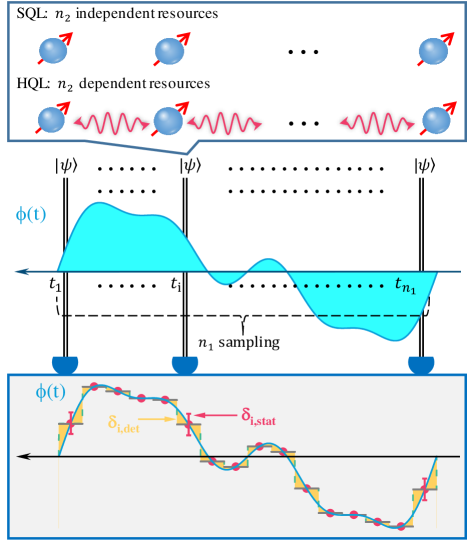
Figure 1: Conceptual diagrams for waveform estimation with ${n_{1}}$ samplings and ${n_{2}}$ independent or correlated quantum resources. The total error includes the deterministic error (golden shadow) and statistical error (red error bar).

In general, we consider the estimation of an unknown waveform $b(t)$ defined over an interval $t\in\left[{0,T}\right]$ with a quantum probe, where $b(t)$ can be stored in a relative phase $\phi(t)$ of its quantum state and sampled using an impulse train of $n_{1}$ impulses, as shown in Fig. 1. The phase $\phi({t_{i}})$ at each moment ${t_{i}}$ is measured by ${n_{2}}$ resources. Finally, we can conveniently generate the waveform estimator $\tilde{\phi}(t)$ with the individual estimators ${\phi(t_{i})}$ by a zero-order hold method Oppenheim et al. (1997); Cooper et al. (2014); Kura and Ueda (2020): $\tilde{\phi}(t)=\sum\nolimits_{i=1}^{{n_{1}}}{{\phi(t_{i})}\theta\left({t-{t_{i}}}\right)}$, where $\theta$ is a smoothing function with $\theta\left(t\right)=1$ for $\left|t\right|\leqslant T/{2n_{1}}$ and $\theta\left(t\right)=0$ otherwise. For a given stochastic estimator $\tilde{\phi}$, the waveform estimation error Kura and Ueda (2020) (see Supplemental Material for details SM (SM)) can be directly decomposed into two parts

$${\delta^{2}}=\delta_{det}^{2}+\delta_{stat}^{2}\text{,}$$ (1)

where ${\delta_{stat}}$ is the statistical error caused by the quantum projection measurement, and ${\delta_{det}}$ is the deterministic error caused by the smoothing process, as shown in Fig. 1. When the waveform is $q$th-order differentiable, ${\delta_{det}}=O\left({n_{1}^{-q}}\right)$ Kura and Ueda (2020); SM (SM). And standard measurement schemes using each resource independently lead to a classical phase uncertainty that scales as ${\delta_{stat}}=O({n}_{2}^{-1/2})$. While, by employing quantum correlations Higgins et al. (2007); Giovannetti et al. (2011); Pezzè et al. (2018); Braun et al. (2018), the quantum enhanced measurements toward ${\delta_{stat}}=O({n}_{2}^{-1})$ will be available. Hence, for a given total number of quantum resources $N={n_{1}}{n_{2}}$, the optimal measurement is determined by the trade-off between these two errors. By employing the inequality of arithmetic and geometric means, the estimation error of arbitrary waveform is bounded by the SQL of $\delta=O\left({{N^{-q/(2q+1)}}}\right)$ and the HQL of $\delta=O\left({{N^{-q/(q+1)}}}\right)$ Kura and Ueda (2020); SM (SM). For the present case $q=1$, the optimal allocation of quantum resource for the best arbitrary waveform estimation can be realized with ${n_{1}}=O\left({{N^{1/3}}}\right)$, ${n_{2}}=O\left({{N^{2/3}}}\right)$ for SQL scheme and ${n_{1}}=O\left({{N^{1/2}}}\right)$, ${n_{2}}=O\left({{N^{1/2}}}\right)$ for HQL scheme.

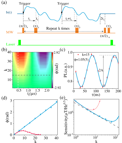
Figure 2: (a) PDD-enhanced TDQD protocol for arbitrary reproducible waveform detection with NV center. (b) The detection of a sinusoidal waveform $b(t)=b\sin\omega t$ with a period of $T=2.4$ $\mu s$. The integration time is $t_{\operatorname{s}}=300$ ns and $\pi$-pulse duration is ${t_{\pi}}=50$ ns. (c) The readout of unknown phase with Rabi oscillation with $k=15$ and $t_{i}=450$ ns, corresponding to the intersection of white and black dashed lines in Fig. 2(b). (d) The accumulation phase as a function of $k$ with the PDD-enhanced (blue circles) and normal Zopes and Degen (2019) (red circles) TDQD protocols. Lines are theoretical results. With the PDD-enhanced TDQD protocol, the solid blue line shows a linear scaling. The uncertainty of phase estimation Dong et al. (2016); Sun et al. (2008); Barry et al. (2020) (error bars) is calculated in a simple way $\Delta{\phi_{k}}=\frac{\sigma}{A}$, where $\sigma$ is signal fluctuation and $A$ is the amplitude of Rabi oscillation as shown in Fig. 2(c). (e) The sensitivity of waveform estimation with the PDD-enhanced (blue circles) and normal (red circles) TDQD protocol. Without taking the decoherence into consideration, the sensitivity scales as the dashed gray line. The best experimental sensitivity (blue dots) is $370$ nT$/\sqrt{Hz}$ for $k=64$.

Here, we experimentally demonstrate the arbitrary reproducible waveform estimation with the negatively charged NV center in diamond Barry et al. (2020); Clevenson et al. (2015); Dong et al. (2018); Chen et al. (2019); Dong et al. (2018); SM (SM), where a substitutional nitrogen atom is next to a vacancy, forming a spin triplet system in its ground state. A room-temperature home-built confocal microscopy is employed to image, initialize and read out the NV center in a single-crystal synthetic diamond sample, which is mounted on a three-axis closed-loop piezoelectric stage for sub-micrometer-resolution scanning. Fluorescence photons are collected into a fiber and detected using single-photon counting module. A copper wire of $10$ $\mu$m diameter above on the bulk diamond is used for the delivery of microwave (MW) and waveform to the NV center. The optical and MW pulse sequences are synchronized by a multichannel pulse generator. Single NV centers are identified by observing anti-bunching in photon correlation measurements.

We perform the waveform estimation by employing a PDD-enhanced TDQD protocol which is based on the differential spin-echo detection Zopes and Degen (2019), as shown in Fig. 2(a). Firstly, we prepare NV center into a probe state $\frac{{\left|0\right\rangle+\left|1\right\rangle}}{{\sqrt{2}}}$. Then, the superposition state evolves under the unknown magnetic field $b\left(t\right)$ along the spin’s quantization axis with a relative phase $\phi(t)=\int_{0}^{t}\gamma_{e}b\left(t\right)dt$, where $\gamma_{e}$ is the gyromagnetic ratio of the spin. We can selectively acquire the phase from the time interval $[t_{i},t_{i}+{t_{s}}]$ while canceling out unwanted dynamically phase evolution by inserting two $\pi$ pulses at times $t_{i}$ and $t_{i}+{t_{s}}$. For ${t_{s}}/T\ll 1$, we have $\phi({t_{i}})\approx-2{\gamma_{e}}b({t_{i}}){t_{s}}$ SM (SM). Finally, the accumulation phase is transferred into the initial phase of Rabi oscillation and measured with optical method. The protocol can be repeated $k$ times to linearly increase the accumulation phase (${\phi_{{n_{2}}}}=k\phi({t_{i}})$). Then, the number of resource used in TDQD protocol is $n_{2}=2k$ for each sampling. To suppress the quantum dephasing effect of ${}^{13}C$ nuclear spins in diamond Dong et al. (2016), we exploit the PDD method by adding a time-delay of $2{t_{s}}$ after the waveform finishing, as shown in Fig. 2(a). In the present case, the quantum dynamic evolution of ${}^{13}C$ nuclear spins under the magnetic field $b(t)$ can be neglected (${\gamma_{{}^{13}C}}b{T_{2}}\ll 1$) and is approximately dominated by the static magnetic field and hyperfine field conditioned on the electron spin state Zhao et al. (2012); SM (SM). The PDD-enhanced TDQD protocol, which is ${\left[{{t_{i}}-\pi-\left({T+{t_{s}}}\right)-\pi-\left({T-{t_{i}}+{t_{s}}}\right)}\right]^{k}}$, consists of a sequence of $\pi$ flips for the sensor evolution. By simply merging the free-evolution propagator term, it turns out to be $\left[{{t_{i}}-PD{D_{k-1}}-\pi-\left({T+{t_{s}}}\right)-\pi-\left({T-{t_{i}}+{t_{s}}}\right)}\right]$, where $PD{D_{k-1}}={\left[{\pi-\left({T+{t_{s}}}\right)-\pi-\left({T+{t_{s}}}\right)}\right]^{k-1}}$. So the experimental signal is $s\sim\exp\left[{-{{\left({\frac{{2k\left({T+{t_{s}}}\right)}}{{{T_{2}}}}}\right)}^{2}}}\right]\cos{\phi_{{n_{2}}}}$ SM (SM).

We first investigate the experimental result by accumulating phase from ${n_{2}}=2k$ consecutive waveform passages. Fig. 2(b) plots the readout of accumulation phase from a weak sinusoidal test signal recorded with different values of $k$. With the increase of $k$, a much stronger oscillation response is observed with a much higher dynamic range Zopes and Degen (2019); Arai et al. (2018). Fig. 2(c) shows the readout process of an unknown accumulation phase with $k=15$ and $t_{i}=450$ ns. Furthermore, we explore the sensor signal as a function of $k$ with a fixed $t_{i}=450$ ns, as shown in Fig. 2(d). For a serial of $k$ values, the accumulation phase is proportional to $k$. Without correcting the decoherence of NV center, we observe the exact linear scaling relationship. The overall sensitivity Zopes and Degen (2019) in the presence of decoherence is also calculated and shown in Fig. 2(e). Obviously, the PDD-enhanced TDQD protocol extends dynamic range and improved the sensitivity of waveform estimation by one order of magnitude comparing with the normal TDQD protocol Zopes and Degen (2019); SM (SM). Besides those advantages, the multi-pulse is also naturally immune to imperfect pulse error operation with phase modulation Genov et al. (2017); Wang et al. (2019).

To demonstrate the superiority of HQL in waveform estimation, we choose a $1$st-order differentiable waveform in the experiment. And more importantly, the balance between ${\delta_{stat}}$ and ${\delta_{\det}}$ should be optimized by tuning the width of smoothing ($t_{s}$). Here, we have an approximate relationship: ${n_{1}}\sim{n_{2}}$ for large $N$, which indicates $\frac{T}{{{t_{s}}+2{t_{\pi}}}}\sim\frac{{{T_{2}}}}{T}$ or $T\approx\sqrt{{T_{2}}\left({{t_{s}}+2{t_{\pi}}}\right)}\approx 10$ $\mu s$, where ${T_{2}=0.66(2)}$ ms SM (SM) is the coherence time of NV center and $T$ is the period of waveform. Here, we choose $T=9.6$ $\mu s$ SM (SM).

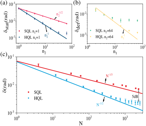
Figure 3: SQL and HQL in waveform estimation. (a) The scaling laws (solid lines) ${\delta_{stat}}=O({n_{2}^{-1/2}})$ for SQL and ${\delta_{stat}}=O({n_{2}^{-1}})$ for HQL, respectively. (b) The deterministic error. The solid golden line shows ${\delta_{det}}=O({n_{1}^{-1}})$. (c) Results of SQL and HQL in waveform estimation. The colored dots represent experimental results. The integration time is ${t_{s}}=\frac{T}{{{n_{2}}}}$ and $T=9.6$ $\mu$s is the period of the sinusoidal waveform.

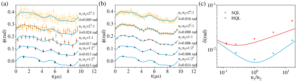
Figure 4: An example of waveform detection with PDD-enhanced TDQD protocol. (a) Results of the SQL scheme. (b) Results of the HQL scheme. The total number of resources is $N={2^{8}}$. The experimental results are shown in stack graph by Y offsets. The input waveform (solid blue line) and the recorded waveform data (colored dots) are given by $b\left(t\right){=b}\left[{{\sin(2}\pi{t/T)+0}{.5\sin(4}\pi{t/T)+0}{.25\sin(8}\pi{t/T)}}\right]$ with $T=9.6$ $\mu s$. (c) Waveform estimation errors (colored dots) with different resource distributions. When the balance between these two errors is broken, the overall waveform estimation errors increase SM (SM).

We test the basic scaling laws ${\delta_{stat}}=O(n_{2}^{-1/2})$ for the SQL with small-interval Ramsey sensing sequence Zopes and Degen (2019); SM (SM) and ${\delta_{stat}}=O(n_{2}^{-1})$ for the HQL in the estimation of a sinusoidal waveform. The experimental results are shown in Fig. 3(a), together with theoretical calculations. The sensitivity of the unknown accumulation phase is therefore increased by $\sqrt{{n_{2}}}$-fold compared with uncorrelated quantum resource, yielding the Heisenberg scaling. Results in Fig. 3(a) also show that as the number of quantum resources further increases when $n\geqslant 64$, ${\delta_{stat}}$ starts to gradually deviate from theoretical values of HQL. This is caused by the decoherence effects (${T_{2}}\sim 64T$) of the NV center SM (SM). However, for the SQL scheme, we can neglect this decoherence effect. Furthermore, the results of $\delta_{det}$ are shown in Fig. 3(b). There is an apparent contradiction between experimental and theoretical results for the SQL scheme because $\delta_{stat}$ is quite large. In this case, noise in waveform reconstruction greatly increases due to the imperfection convergency of experimental data and the relationship ${\delta_{det}}=O\left({n_{1}^{-1}}\right)$ will be overwhelmed by noise. However, this type of error is reduced by employing HQL scheme and the basic scaling laws ${\delta_{det}}=O({n_{1}^{-1}})$ emerges. When $\delta_{stat}$ deviates from the theoretical prediction under decoherence, $\delta_{det}$ will also deviate from $O({n_{1}^{-1}})$. So these two kinds of estimation errors are tangled up in the experiment for the waveform reconstruction. By making use of the inequality of arithmetic and geometric means, the trade-off between ${\delta_{stat}}$ and ${\delta_{det}}$ can be optimized numerically SM (SM). Fig. 3(c) shows this key experimental results of overall waveform estimation errors. For the $1$st-order differentiable waveform estimation, the fundamental limits bounded by $\delta{\text{ = }}O\left({{N^{-1/3}}}\right)$ for SQL and $\delta{\text{ = }}O\left({{N^{-1/2}}}\right)$ for HQL are experimentally demonstrated. The HQL-scaled waveform estimation based on the PDD-enhanced TDQD protocol clearly demonstrates the superiority of quantum metrology. For example, we have demonstrated the use of $\sim 2\times{{\text{10}}^{3}}$ resources to achieve the waveform estimation error $5$ dB below the SQL. While more than ${1\times{\text{1}}{{\text{0}}^{5}}}$ resources would be required to achieve a similar error level using standard classical techniques.

We further complete our study by demonstrating the reconstruction of a complex test waveform, which contains the sum of several frequency components. The experimentally measured waveform in SQL and HQL scheme together with the input waveform are shown in Fig. 4(a) and (b), respectively. With the same number of resources, the superiority of HQL scheme for waveform estimation is observed clearly in the experiment. By employing quantum correlation with the PDD-enhanced TDQD protocol, the statistical error is reduced and the measurement results converge to the ideal value quickly. Clearly, the overall waveform estimation error $\delta$ is changed with the proportion of resource distribution. For a given number of resource $N=n{{}_{1}}{n_{2}}$, the optimal accuracy is determined by the trade-off between ${\delta_{stat}}$ and ${\delta_{det}}$, as shown in Fig. 4(c). When ${n_{1}}\sim{n_{2}}$, the optimal waveform reconstruction of $q=1$ is realized in HQL scheme with NV center. A similar relationship also applies to the SQL case SM (SM).

In summary, we present a PDD-enhanced TDQD protocol for Heisenberg-limited arbitrary reproducible waveform estimation. The current results demonstrate the potential of the quantum measurement technique, which is readily available for other quantum probe systems Degen et al. (2017); Mitchell and Palacios Alvarez (2020); Pirandola et al. (2018). For the $1$st-order differentiable arbitrary waveform, we demonstrate the SQL of $O\left({{N^{{-}1/3}}}\right)$ and the HQL of $O\left({{N^{{-}1/2}}}\right)$ in the experiment, which is significantly different with previous parametric estimation. This new fundamental result sets a new quantum-enhanced metrology scaling law of high precision detection of continuous physical signals Abadie et al. (2011); Kura and Ueda (2020); Cooper et al. (2014). And far more than physical scope, the estimation of continuous signals and images in micro-fluidic chemical analysis Lim et al. (2015), vital activity Michalet et al. (2005); Barry et al. (2016) and pattern recognition Wang et al. (2018) in computer science would be significantly improved by making use of the quantum superiority. Moreover, the waveform sampling based on the TDQD protocol will benchmark the quantum version of the Nyquist-Shannon sampling theorem Kura and Ueda (2020), which would directly knock on the door of the practical quantum oscilloscope.

Beyond the current work, multiple entangled state Pirandola et al. (2018); Omran et al. (2019); Song et al. (2019); Han et al. (2020) can be applied to achieve same quantum-enhanced waveform estimation with parallel schemes. And more general unpredictable signal can be detected at one time. For the TDQD and parallel schemes, same quantum coherent amplification of unknown phase can be realized and the detection resolution can reach the Heisenberg-limited scaling. That is the quantum Cramér-Rao bound can be asymptotically approached in both cases. Here, the equivalence between entanglement in parallel schemes and coherence (namely, superposition in the eigenbasis of the generator) can be understood by observing that both nonclassicality in infinite-dimensional systems and coherence (superposition) in finite-dimensional systems can be converted to entanglement within a well-defined resource-theoretic framework Braun et al. (2018); Nishioka (2018). This precise understanding and control of genuine quantum effects such as nonclassicality and superposition will further extend the application of quantum metrology in the future.

This work is supported by the National Key Research and Development Program of China (Grant No. 2017YFA0304504), the National Natural Science Foundation of China (Grants No. 91536219, No. 61522508, and No. 91850102), the Anhui Initiative in Quantum Information Technologies (Grant No. AHY130000), the Science Challenge Project (Grant No. TZ2018003), and the Fundamental Research Funds for the Central Universities (No. WK2030000020).

References

- Giovannetti et al. (2011) V. Giovannetti, S. Lloyd, and L. Maccone, Nat. Photonics 5, 222 (2011).
- Pezzè et al. (2018) L. Pezzè, A. Smerzi, M. K. Oberthaler, R. Schmied, and P. Treutlein, Rev. Mod. Phys. 90, 035005 (2018).
- Braun et al. (2018) D. Braun, G. Adesso, F. Benatti, R. Floreanini, U. Marzolino, M. W. Mitchell, and S. Pirandola, Rev. Mod. Phys. 90, 035006 (2018).
- Pirandola et al. (2018) S. Pirandola, B. R. Bardhan, T. Gehring, C. Weedbrook, and S. Lloyd, Nat. Photonics 12, 724 (2018).
- Sun et al. (2008) F. W. Sun, B. H. Liu, Y. X. Gong, Y. F. Huang, Z. Y. Ou, and G. C. Guo, EPL 82, 24001 (2008).
- Higgins et al. (2007) B. L. Higgins, D. W. Berry, S. D. Bartlett, H. M. Wiseman, and G. J. Pryde, Nature 450, 393 (2007).
- Dong et al. (2016) Y. Dong, X.-D. Chen, G.-C. Guo, and F.-W. Sun, Phys. Rev. A 94, 052322 (2016).
- Kessler et al. (2014) E. M. Kessler, I. Lovchinsky, A. O. Sushkov, and M. D. Lukin, Phys. Rev. Lett. 112 (2014).
- Streltsov et al. (2017) A. Streltsov, G. Adesso, and M. B. Plenio, Rev. Mod. Phys. 89, 041003 (2017).
- Dong et al. (2018) Y. Dong, Y. Zheng, S. Li, C.-C. Li, X.-D. Chen, G.-C. Guo, and F.-W. Sun, npj Quantum Inf. 4, 3 (2018).
- Nishioka (2018) T. Nishioka, Rev. Mod. Phys. 90, 035007 (2018).
- Dong et al. (2019) Y. Dong, X.-D. Chen, G.-C. Guo, and F.-W. Sun, Phys. Rev. B 100, 214103 (2019).
- Han et al. (2020) B. Han, J. Duan, S. Jin, X. Lu, P. Li, W. Qu, M. Wang, N. Irina, E. E. Mikhailov, Z. Kai-Feng, et al., Nature 581, 159 (2020).
- Pan et al. (2012) J.-W. Pan, Z.-B. Chen, C.-Y. Lu, H. Weinfurter, A. Zeilinger, and M. Żukowski, Rev. Mod. Phys. 84, 777 (2012).
- Hou et al. (2019) Z. Hou, R.-J. Wang, J.-F. Tang, H. Yuan, G.-Y. Xiang, C.-F. Li, and G.-C. Guo, Phys. Rev. Lett. 123, 040501 (2019).
- Motes et al. (2015) K. R. Motes, J. P. Olson, E. J. Rabeaux, J. P. Dowling, S. J. Olson, and P. P. Rohde, Phys. Rev. Lett. 114, 170802 (2015).
- Monz et al. (2011) T. Monz, P. Schindler, J. T. Barreiro, M. Chwalla, D. Nigg, W. A. Coish, M. Harlander, W. Hänsel, M. Hennrich, and R. Blatt, Phys. Rev. Lett. 106, 130506 (2011).
- Omran et al. (2019) A. Omran, H. Levine, A. Keesling, G. Semeghini, T. T. Wang, S. Ebadi, H. Bernien, A. S. Zibrov, H. Pichler, S. Choi, et al., Science 365, 570 (2019).
- Song et al. (2019) C. Song, K. Xu, H. Li, Y.-R. Zhang, X. Zhang, W. Liu, Q. Guo, Z. Wang, W. Ren, J. Hao, et al., Science 365, 574 (2019).
- Bradley et al. (2019) C. E. Bradley, J. Randall, M. H. Abobeih, R. C. Berrevoets, M. J. Degen, M. A. Bakker, M. Markham, D. J. Twitchen, and T. H. Taminiau, Phys. Rev. X 9, 031045 (2019).
- Liu et al. (2015) G.-Q. Liu, Y.-R. Zhang, Y.-C. Chang, J.-D. Yue, H. Fan, and X.-Y. Pan, Nat. Commun. 6, 6726 (2015).
- Abadie et al. (2011) J. Abadie, B. Abbott, R. Abbott, T. D. Abbott, M. R. Abernathy, C. Adams, R. X. Adhikari, C. Affeldt, B. Allen, G. S. Allen, et al., Nat. Phys. 7, 962 (2011).
- Kura and Ueda (2020) N. Kura and M. Ueda, Phys. Rev. Lett. 124, 010507 (2020).
- Cooper et al. (2014) A. Cooper, E. Magesan, H. N. Yum, and P. Cappellaro, Nat. Commun. 5, 3141 (2014).
- Zopes and Degen (2019) J. Zopes and C. Degen, Phys. Rev. Appl. 12, 054028 (2019).
- Michalet et al. (2005) X. Michalet, F. Pinaud, L. Bentolila, J. Tsay, S. Doose, J. Li, G. Sundaresan, A. Wu, S. Gambhir, and S. Weiss, Science 307, 538 (2005).
- Budker and Romalis (2007) D. Budker and M. Romalis, Nat. Phys. 3, 227 (2007).
- Brida et al. (2010) G. Brida, M. Genovese, and I. R. Berchera, Nat. Photonics 4, 227 (2010).
- Samantaray et al. (2017) N. Samantaray, I. Ruo-Berchera, A. Meda, and M. Genovese, Light Sci. Appl. 6, e17005 (2017).
- Akiyama et al. (2019a) K. Akiyama, A. Alberdi, W. Alef, K. Asada, R. Azulay, A.-K. Baczko, D. Ball, M. Balokovic, J. Barrett, D. Bintley, et al., Astrophys. J. 875, L3 (2019a).
- Akiyama et al. (2019b) K. Akiyama, A. Alberdi, W. Alef, K. Asada, R. Azulay, A.-K. Baczko, D. Ball, M. Balokovic, J. Barrett, D. Bintley, et al., Astrophys. J. 875, L4 (2019b).
- Chen et al. (2018) G. Chen, L. Zhang, W.-H. Zhang, X.-X. Peng, L. Xu, Z.-D. Liu, X.-Y. Xu, J.-S. Tang, Y.-N. Sun, D.-Y. He, et al., Phys. Rev. Lett. 121, 060506 (2018).
- Kitagawa and Ueda (1993) M. Kitagawa and M. Ueda, Phys. Rev. A 47, 5138 (1993).
- Zhang et al. (2017) Y.-C. Zhang, X.-F. Zhou, X. Zhou, G.-C. Guo, and Z.-W. Zhou, Phys. Rev. Lett. 118, 083604 (2017).
- Kuzyk and Wang (2018) M. C. Kuzyk and H. Wang, Phys. Rev. X 8, 041027 (2018).
- Oppenheim et al. (1997) A. V. Oppenheim, A. S. Willsky, and S. Hamid, Signals and Systems (Prentice Hall, Englewood Cliffs, NJ, 1997).
- SM (SM) See Supplemental Material at [] for the calculation of estimation error of waveform, intruduction to the NV center, experimental setup, TDQD and PDD-enhanced TDQD protocol, and the optimal resource allocation of SQL and HQL schemes, which includes Refs. [38-40].
- Souza et al. (2011) A. M. Souza, G. A. Álvarez, and D. Suter, Phys. Rev. Lett. 106, 240501 (2011).
- Herbschleb et al. (2019) E. D. Herbschleb, H. Kato, Y. Maruyama, T. Danjo, T. Makino, S. Yamasaki, I. Ohki, K. Hayashi, H. Morishita, M. Fujiwara, et al., Nat. Commun. 10, 3766 (2019).
- Nocedal and Wright (2006) J. Nocedal and S. J. Wright, Numerical Optimization (Springer, New York, 2006).
- Barry et al. (2020) J. F. Barry, J. M. Schloss, E. Bauch, M. J. Turner, C. A. Hart, L. M. Pham, and R. L. Walsworth, Rev. Mod. Phys. 92, 015004 (2020).
- Clevenson et al. (2015) H. Clevenson, M. E. Trusheim, C. Teale, T. Schroeder, D. Braje, and D. Englund, Nat. Phys. 11, 393 (2015).
- Chen et al. (2019) X.-D. Chen, D.-F. Li, Y. Zheng, S. Li, B. Du, Y. Dong, C.-H. Dong, G.-C. Guo, and F.-W. Sun, Phys. Rev. Appl. 12, 044039 (2019).
- Dong et al. (2018) Y. Dong, S.-C. Zhang, H.-B. Lin, X.-D. Chen, W. Zhu, G.-Z. Wang, G.-C. Guo, and F.-W. Sun, arXiv:2003.02472 (2020).
- Zhao et al. (2012) N. Zhao, S.-W. Ho, and R.-B. Liu, Phys. Rev. B 85, 115303 (2012).
- Arai et al. (2018) K. Arai, J. Lee, C. Belthangady, D. R. Glenn, H. Zhang, and R. L. Walsworth, Nat. Commun. 9, 4996 (2018).
- Genov et al. (2017) G. T. Genov, D. Schraft, N. V. Vitanov, and T. Halfmann, Phys. Rev. Lett. 118, 133202 (2017).
- Wang et al. (2019) Z.-Y. Wang, J. E. Lang, S. Schmitt, J. Lang, J. Casanova, L. McGuinness, T. S. Monteiro, F. Jelezko, and M. B. Plenio, Phys. Rev. Lett. 122 (2019).
- Degen et al. (2017) C. L. Degen, F. Reinhard, and P. Cappellaro, Rev. Mod. Phys. 89, 035002 (2017).
- Mitchell and Palacios Alvarez (2020) M. W. Mitchell and S. Palacios Alvarez, Rev. Mod. Phys. 92, 021001 (2020).
- Lim et al. (2015) K. Lim, C. Ropp, B. Shapiro, J. M. Taylor, and E. Waks, Nano Lett. 15, 1481 (2015).
- Barry et al. (2016) J. F. Barry, M. J. Turner, J. M. Schloss, D. R. Glenn, Y. Song, M. D. Lukin, H. Park, and R. L. Walsworth, Proc. Natl. Acad. Sci. 113, 14133 (2016).
- Wang et al. (2018) Z. Wang, S. Joshi, S. Savel’ev, W. Song, R. Midya, Y. Li, M. Rao, P. Yan, S. Asapu, Y. Zhuo, et al., Nat. Electron. 1, 137 (2018).