In Wigner phase space, convolution explains why the vacuum majorizes mixtures of Fock states

Abstract

I show that a nonnegative Wigner function that represents a mixture of Fock states is majorized by the Wigner function of the vacuum state. As a consequence, the integration of any concave function over the Wigner phase space has a lower value for the vacuum state than for a mixture of Fock states. The Shannon differential entropy is an example of such concave function of significant physical importance. I demonstrate that the very cause of the majorization lies in the fact that a Wigner function is the result of a convolution. My proof is based on a new majorization result dedicated to the convolution of the negative exponential distribution with a precisely constrained function. I present a geometrical interpretation of the new majorization property in a discrete setting and extend this relation to a continuous setting. Findings presented in this article might be expanded upon to explain why the Wigner function of the vacuum majorizes - beyond mixtures of Fock states - many other physical states represented by a nonnegative Wigner function.

1 Introduction

Phase space representations were conceived almost ninety years ago by Eugene Wigner [1]. Although the original application was the description of states and systems in Quantum mechanics, the Wigner function is today a successful tool in areas as diverse as the study of radiation and optical systems [2], quantum electronics, quantum chemistry or signal analysis [1]. The Wigner phase space has also proved to be an efficient framework in the analysis of both stationary and time-dependent systems.

The Wigner function keeps providing interesting insight when analysing quantum systems. This is also strengthened by the fact that the Wigner function has a series of - almost directly visible - features that nicely reflect the physics of the quantum states they represent. For instance, negative parts in the Wigner functions are viewed as the signature of a non-classical behaviour [3], whereas in the absence of negative areas, it behaves as an actual probability distribution. Another illustration is the normalization of the Wigner function that simply mirrors the unit trace of the density operator.

The entropy of the Wigner function - and more specifically Shannon differential entropy - is a quantity that relates to the amount of information that can be gained on a quantum system. When entropy relations involve the two variables of the two-dimensional Wigner phase space, they can reflect the limited amount of knowledge that can be obtained simultaneously on both variables. For instance, some lower bounds on the sum of the entropies of the two phase space variables imply Heisenberg’s uncertainty relations [4, 5].

It has been conjectured that the joint entropy of the Wigner function of a coherent state is the minimum joint entropy that any physical state can have if it is represented by a nonnegative Wigner function [5]. Visually, this would mean that a Wigner function can never be “more peaked” than the Wigner function of a coherent state.

In this article, I prove this conjecture for the case of mixtures of Fock states. I use the theory of majorization and I explain why the Wigner function of the vacuum state majorizes the Wigner function of mixtures of Fock states - in the cases where this Wigner function is nonnegative. Such majorization relation directly implies entropy (and seminorms) comparisons between the various distributions.

In section 2, I start by rewriting a couple of definitions and properties that I use in this article. The seven parts of my proof are presented in section 3. Section 4 details the proof of the two main theorems of this article and I conclude in section 5.

2 Definitions and Properties

In this article, a vector $x$ is said to be nonnegative if all its elements are nonnegative $x_{i}\geqslant 0,\>\forall i$. A vector is said to be normalized if the sum of its elements is equal to $1$. Similarly, in the continuous case, a function $f\left(x\right)$ defined on the measure space $\left(H,\mathscr{I},\nu\right)$ is said to be nonnegative if it takes nonnegative values on its domain $H$. A function $f\left(x\right)$ is said to be normalized if

$$\intop f(x)\;\mathrm{d}\nu(x)=1,$$

where the integration is performed over the complete domain $H$.

Some Definitions of Majorization

I first recall a couple of equivalent definitions for majorization, both in a discrete setting and in a continuous setting. I restrict the description of the equivalent definitions to the ones that will be used in this article.

In a discrete setting, if $x$,$\>y\in\mathbb{R}^{N}$, the following five statements are equivalent [6, 7]:

1. The vector $x$ majorizes $y$, denoted $x\succ y$.

2. $$\sum_{i=1}^{k}x_{i}^{\downarrow}\geqslant\sum_{i=1}^{k}y_{i}^{\downarrow}, \qquad k=1,\dots,N-1,\qquad\text{and}$$ (1a)

   $$\sum_{i=1}^{N}x_{i}=\sum_{i=1}^{N}y_{i},$$ (1b)

   where the vectors $x{}^{\downarrow}$ and $y{}^{\downarrow}$ include the same elements, respectively as $x$ and $y$, but re-sorted in a non-increasing order.

3. $$\sum_{i=1}^{N}\Phi\left(x_{i}\right)\geqslant\sum_{i=1}^{N}\Phi\left(y_{i}\right),$$ (2)

   for all continuous convex functions $\Phi:\mathbb{R}\longrightarrow\mathbb{R}$.

4. There exists a $N\times N$ doubly stochastic matrix $D$ such that

   $$y=Dx.$$ (3)

5. The vector $y$ can be derived from $x$ by performing a limited number of Robin Hood transfers. A transfer of a positive amount $\Delta$ from $x{}_{i}$ to $x{}_{j}$, giving $y_{i}=x_{i}-\Delta$ and $y_{j}=x_{j}+\Delta$ is said to be a Robin Hood transfer if $\Delta\leqslant x_{i}-x_{j}$. This definition is valid for nonnegative vectors $x$ and $y$. A Robin Hood transfer is also called a Dalton transfer or sometimes a “pinch” [7].

Similarly, in a continuous setting, if $f$ and $g$ are nonnegative $\nu$-integrable functions defined on the measure space $\left(H,\mathscr{I},\nu\right)$, the following four statements are equivalent [8, 7]:

1. The function $f$ majorizes $g$, denoted $f\succ g$.

2. $$\intop_{0}^{t}f_{\downarrow}(u)\;\mathrm{d}\nu(u)\geqslant\intop_{0}^{t}g_{\downarrow}(u)\;\mathrm{d}\nu(u), \qquad\forall t\in\left[0,\nu\left(H\right)\right)\quad\text{and}$$ (4a)

   $$\intop f(u)\;\mathrm{d}\nu(u)=\intop g(u)\;\mathrm{d}\nu(u),$$ (4b)

   where $f_{\downarrow}$ (and identically for $g_{\downarrow}$) denotes the decreasing rearrangement of $f$ defined in two steps:

   $$m_{f}(t)=\nu\left(\left\{x:f\left(x\right)>t\right\}\right), \qquad t\geqslant 0,\qquad\text{and},$$ (5a)

   $$f_{\downarrow}(u)=\sup\left\{t:m_{f}(t)>u\right\}, \qquad 0\leqslant u\leqslant\nu\left(H\right).$$ (5b)

3. $$\intop\Phi(f)\;\mathrm{d}\nu\geqslant\intop\Phi(g)\;\mathrm{d}\nu,$$ (6)

   for all continuous convex functions $\Phi:\mathbb{R}\longrightarrow\mathbb{R}$ with $\Phi\left(0\right)=0$, for which the integrals exist.

4. $$g(y)=\intop k\left(x,y\right)\>f\left(x\right)\>\mathrm{d}\nu\left(x\right)$$ (7)

   where $k:\>H\times H\longrightarrow\left[0,+\infty\right)$ is a doubly stochastic function, that is, $\intop k\left(x,y\right)\>\mathrm{d}\nu\left(x\right)=1$ for all $y\in H$ and $\intop k\left(x,y\right)\>\mathrm{d}\nu\left(y\right)=1$ for all $x\in H$. Note that some authors present this condition as sufficient and not as an equivalent definition [8]. In this article, Eq. (7) is only used as a sufficient condition for majorization.

A number of properties of discrete majorization extend to continuous majorization and we note the similarities between the equivalent definitions in the discrete and in the continuous settings (not all are reproduced here). In the continuous setting, some of the equivalent definitions are applicable to nonnegative functions; this nonnegativity restriction can be relaxed if $\nu\left(H\right)$ is finite [7]. I keep this restriction as the support of the functions studied in this article is not finite.

Majorization Property of the Convolution of Two Probability Distributions

The convolution vector of two probability distributions is majorized by the two original probability distributions [6]. I particularize here the proof [6, 7] to the case where the first probability vector has one more element than the second probability vector. The discrete convolution of a normalized vector $y=\left(y{}_{1},y{}_{2},\dots,y_{N+1}\right)^{\intercal}$ and a vector $x=\left(x{}_{1},x{}_{2},\dots,x_{N}\right)^{\intercal}$ is formulated as the multiplication by a Toeplitz matrix constructed as follows:

$$z=y\ast x=\left(\begin{array}[]{cccc}y{}_{1}&0&\cdots&0\\ y{}_{2}&y{}_{1}&\ddots&\vdots\\ \vdots&y{}_{2}&\ddots&0\\ y{}_{N}&\vdots&\ddots&y{}_{1}\\ y{}_{N+1}&y{}_{N}&\ddots&y{}_{2}\\ 0&y{}_{N+1}&\ddots&\vdots\\ \vdots&\ddots&\ddots&y{}_{N}\\ 0&\cdots&0&y{}_{N+1}\end{array}\right)\left(\begin{array}[]{c}x{}_{1}\\ x{}_{2}\\ \vdots\\ x{}_{N}\end{array}\right),$$ (20)

where the symbol $\ast$ denotes the convolution. The resulting probability vector $z$ has a maximum of $2N$ non-zero elements. If we build a $2N\times 2N$ circulant matrix $C$ by adding $N$ columns at the right of the above Toeplitz matrix, the probability vector $z$ can also be written as

$$z=C\left(\begin{array}[]{c}x{}_{1}\\ x{}_{2}\\ \vdots\\ x{}_{N}\\ 0\\ 0\\ \vdots\\ 0\end{array}\right),$$ (29)

where $N$ zero elements are added to the vector $x$. With Eq. (3), the equality in Eq. (29) proves that $x\succ z$ because the circulant matrix $C$ is doubly stochastic.

These results have been generalized to the continuous distributions. In particular, if $X$ and $Y$ are independent random variables with absolutely continuous distribution functions, then the distribution of $X+Y$ is majorized by both the distributions of $X$ and $Y$ [8] - the explicit proof is not provided in the referenced article.

If $c,\>f:\>\mathbb{R}^{+}\longrightarrow\mathbb{R}$ are two functions whose support is the positive real axis, the convolution of $c\left(x\right)$ and $f\left(x\right)$ is

$$g\left(x\right)=c\ast f=\intop_{0}^{x}c\left(t\right)f\left(x-t\right)\mathrm{d}t, \qquad x\geqslant 0.$$ (30)

A discrete version of this integral matches the formulation involving the Toeplitz matrix of Eq. (20).

The Wigner Function of the Fock States

The definition of the Wigner function of the quantum state with density operator $\hat{\rho}$ is [9]

$$W(x,p)=\frac{1}{2\pi}\intop_{-\infty}^{+\infty}\>\langle x-\frac{x^{\prime}}{2}|\hat{\rho}|p+\frac{x^{\prime}}{2}\rangle\>e^{ix^{\prime}p}\>\mathrm{d}x^{\prime},$$ (31)

where $x$ and $p$ are canonically conjugate variables.

With this dimensionless definition, the Wigner function of the eigenstate of the Number operator with integer eigenvalue $n$ reads [9]

$$W_{n}(r,\theta)=\tilde{W}_{n}(r^{2})=\frac{\left(-1\right)^{n}}{\pi}\>L_{n}\left(2r^{2}\right)\>e^{-r^{2}},$$ (32)

where $r$ and $\theta$ are the polar coordinates in Wigner phase space and $L_{n}\left(x\right)$ denotes the Laguerre polynomial of the $n$-th order. The eigenstates of the Number operator are referred to as Fock states and the state corresponding to $n=0$ as the vacuum state.

A Set of States with Nonnegative Wigner Function

Some recent results about nonnegative Wigner functions will be used in my proof. When injecting the Fock states $|m\rangle$ and $|n\rangle$ into the two inputs of a balanced beamsplitter, the states at each of the two outputs of the balanced beamsplitter can be written as the following mixture of Fock states [10, 11]:

$$\hat{\sigma}\left(m,n\right)=\left(m!\,n!\,2^{m+n}\right)^{-1}\>\sum_{z=0}^{m+n}\sum_{i=max\left(0,z-n\right)}^{min\left(z,m\right)}\;\sum_{j=max\left(0,z-n\right)}^{min\left(z,m\right)}\;\left(-1\right)^{i+j}\qquad\qquad$$

$$\times\left(\begin{array}[]{c}m\\ i\end{array}\right)\left(\begin{array}[]{c}n\\ z-i\end{array}\right)\left(\begin{array}[]{c}m\\ j\end{array}\right)\left(\begin{array}[]{c}n\\ z-j\end{array}\right)\>z!\,\left(m+n-z\right)!\quad|z\rangle\langle z|.$$ (41)

It was proved that the states $\hat{\sigma}\left(m,n\right)$ have a nonnegative Wigner function [10]. For more details about the generation and properties of the states $\hat{\sigma}\left(m,n\right)$, I refer the reader to the article [10] and to the articles cited therein.

In the present article, I will use Eq. (41) as the definition of a parameterized set of states that have a nonnegative Wigner function.

3 Proof

In this section, I prove that the Wigner function of the vacuum majorizes the Wigner function of any mixture of Fock states when the latter Wigner function is nonnegative. The proof consists of seven parts.

Definition 1

In the Wigner phase space, the Wigner function $W_{\alpha}$ majorizes $W_{\beta}$, denoted as $W_{\alpha}\underset{W}{\succ}W_{\beta}$, if

$$\intop\Phi(W_{\alpha}\left(\vec{s}\right))\;\mathrm{d}\vec{s}\;\geqslant\intop\Phi(W_{\beta}\left(\vec{s}\right))\;\mathrm{d}\vec{s},$$ (42)

for all continuous convex functions $\Phi:\mathbb{R}\longrightarrow\mathbb{R}$ with $\Phi\left(0\right)=0$, for which the integrals over the complete $2$-dimensional phase space exist.

For Wigner functions that do not depend on the angular coordinate but only depend on the radial coordinate $r$, the majorization in Eq. (42) is an application of the definition in Eq. (6) with the measure $\nu=r^{2}$. I use the index $W$ below the majorization symbol in $W_{\alpha}\underset{W}{\succ}W_{\beta}$ to refer to the majorization with respect to the measure $\nu=r^{2}$.

In this article, I study convex combinations of Fock states and I only consider Wigner functions that depend on $r^{2}$, as defined in Eq. (32). A direct application of the definition in Eq. (42) to two such functions, $W_{\alpha}=W_{\alpha}\left(r^{2}\right)$ and $W_{\beta}=W_{\beta}\left(r^{2}\right)$ shows that

$$W_{\alpha}\left(r^{2}\right)\underset{W}{\succ}W_{\beta}\left(r^{2}\right) \iff W_{\alpha}\left(z\right)\succ W_{\beta}\left(z\right),$$ (43)

where the change of variable $z=r^{2}$ was performed. The majorization on the right-hand side of Eq. (43) is the majorization with respect to the usual measure, that is, $\nu\left(z\right)=z$. The domain of definition of the functions $W_{\alpha}\left(z\right)$ and $W_{\beta}\left(z\right)$ is $\left[0,+\infty\right)$. As an example, to compare the Wigner function of the vacuum and the Wigner function of an equally weighted mixture of the first two Fock states, we can write

$$W_{0}\underset{W}{\succ}\frac{1}{2}\left(W_{0}+W_{1}\right) \iff e^{-z}\succ ze^{-z},$$ (44)

where $z\in\mathbb{R}^{+}$.

Formulation as a Convolution

Thanks to Eq. (43), to obtain a majorization relation between the vacuum and the Wigner function $W_{\beta}\left(r^{2}\right)$ of a convex combination of Fock states, we can compare $W_{\alpha}\left(z\right)=e^{-z}$ with $W_{\beta}\left(z\right)$. To perform this comparison, it will prove useful to formulate $W_{\beta}\left(z\right)$ as a convolution.

Eq. (32) of a Fock state shows that $W_{\beta}\left(z\right)$ is the product of a polynomial with $e^{-z}$ denoted here by $W_{\beta}\left(z\right)=P\left(z\right)e^{-z}$.

The expression $P\left(z\right)e^{-z}$ can also be viewed as a linear combination of Erlang distributions of rate parameter equal to $1$. The support of the Erlang distribution is $\mathbb{R}^{+}$ and its general expression is

$$E_{k+1}(z)=\frac{z^{k}e^{-z}}{k!}=p_{k}(z)e^{-z}, \qquad k=0,1,2\dots\quad\text{and}\quad z\geqslant 0,$$ (45)

which defines $p_{k}(z)$. The Erlang distribution of shape parameter $k+1$ is the convolution as defined by Eq. (30), of an Erlang distribution of shape parameter $k$ with the negative exponential distribution. If I also introduce the derivative of the polynomial $p_{k}(z)$, for $k\geqslant 1$,

$$p_{k}(z)e^{-z}=E_{k+1}(z)=E_{k}(z)\ast e^{-z}=\left(p_{k}^{\prime}(z)e^{-z}\right)\ast e^{-z}, \quad z\geqslant 0.$$ (46)

$P\left(z\right)$ is a linear combination of the $p_{k}(z)$ and Eq. (46) gives

$$P\left(z\right)e^{-z}=\sum_{k=0}^{+\infty}a_{k}p_{k}(z)e^{-z}=a_{0}e^{-z}+\left(\sum_{k=1}^{+\infty}a_{k}p_{k}^{\prime}(z)e^{-z}\right)\ast e^{-z}, \quad z\geqslant 0.$$ (47)

The function $W_{\beta}\left(z\right)$ can finally be formulated as the following convolution:

$$W_{\beta}\left(z\right)=P\left(z\right)e^{-z}=\left(a_{0}\delta\left(z\right)+P^{\prime}\left(z\right)e^{-z}\right)\ast e^{-z}, \quad z\geqslant 0,$$ (48)

where the Dirac delta function takes the term $k=0$ of the sum into account and $a_{0}$ was implicitly defined in Eq. (47) as the zero order coefficient of $P\left(z\right)$.

Note that the fact that $E_{k+1}(z)$ is obtained from the convolution of the distributions $E_{k}(z)$ and $e^{-z}$ implies that $P\left(z\right)e^{-z}\prec e^{-z}$ in the cases where the coefficients of the polynomial $P\left(z\right)$ are nonnegative [8]. This proves for instance that $W_{0}\underset{W}{\succ}\frac{1}{2}\left(W_{0}+W_{1}\right)$.

Eq. (48) actually provides an indirect representation of $W_{\beta}\left(r^{2}\right)$ as the convolution of a continuous function (except in $z=0$) with the negative exponential $e^{-z}$ that represents the vacuum.

Theorem 1

Theorem 1 is a new majorization property applicable to the convolution of a discrete negative exponential $v{}_{0}$ with a vector $x$ that can have negative elements.

Let the non-normalized vector $v{}_{0}=\left(a^{0},a^{1},a^{2},\dots,a^{N-1}\right){}^{\intercal}$ with $0<a<1$ and let $x$ be a normalized $N+1$-dimensional vector that can be written as the sum

$$x^{\intercal}=\left(1,0,\dots,0\right)+\sum_{k=1}^{N}\left(0,\dots,0,-\lambda_{k},\lambda_{k},0,\dots,0\right),$$ (49)

where $\lambda_{k}\geqslant 0,\;k=1,\dots,N$, and the $k$-th and $k+1$-th elements are the only non-zero elements of each vector in the sum of Eq. (49).

Let $G$ be the $2N$-dimensional vector defined by the convolution $G=x\ast v_{0}$. My main theorem states that

$$\text{If }\;G\geqslant 0\;\text{ Then }\;v_{0}\succ G.$$ (50)

The proof of Theorem 1 is provided in section 4.

Lemma 1

A vector $x\in\mathbb{R}^{N+1}$ can be decomposed into a sum of the form

$$x^{\intercal}=\left(\lambda_{0},0,\dots,0\right)+\sum_{k=1}^{N}\left(0,\dots,0,-\lambda_{k},\lambda_{k},0,\dots,0\right),$$ (51)

where all $\lambda_{k}\geqslant 0$, if and only if

$$\sum_{i=k}^{N}x_{i}\geqslant 0,\qquad k=0,\dots,N.$$ (52)

To first prove the inverse implication, it suffices to decompose the vector $x$ into a sum of terms of the form $\left(0,\dots,0,-\lambda_{k},\lambda_{k},0,\dots,0\right)^{\intercal}$, which also proves the unicity of the decomposition. As per Eq. (52), $x{}_{N}$ is positive and the last term of the sum must be $\left(0,\dots,0,-x_{N},x_{N}\right)^{\intercal}$. Eq. (52) directly shows that the $k$-th term $\left(0,\dots,0,-\sum_{i=k}^{N}x_{i},\sum_{i=k}^{N}x_{i},0,\dots,0\right)^{\intercal}$ of the decomposition has the form required in Eq. (51). Finally, because $\lambda_{0}=\sum_{i=0}^{N}x_{i}$, the parameter $\lambda_{0}\geqslant 0$ and $\lambda_{0}=1$ if the vector $x$ is normalized.

The direct implication derives from the fact that a single vector of the form $\left(0,\dots,0,-\lambda_{k},\lambda_{k},0,\dots,0\right)^{\intercal}$ with $\lambda_{k}\geqslant 0$ satisfies Eq. (52) and that the sum of vectors that satisfies Eq. (52) also satisfies that same equation.

Theorem 2

Theorem 2 is the extension of Theorem 1 - combined with Lemma 1 - to the continuous case.

Let $c(z)$ be a function defined on $\left[0,+\infty\right)$, integrable and continuous on its domain, except in $z=0$ where one term of the function $c(z)$ can be proportional to a Dirac delta function. The function $c(z)$ also fulfills the conditions

$$\intop_{x}^{+\infty}\;c\left(z\right)\;\mathrm{d}z\geqslant 0, \qquad\forall\>x>0$$ and (53a)

$$\intop_{0}^{+\infty}\;c\left(z\right)\;\mathrm{d}z=1.$$ (53b)

Let $e^{-z}$ denote the negative exponential distribution defined on $\left[0,+\infty\right)$ and let the function $g$ be the convolution $g\left(z\right)=c\left(z\right)\ast e^{-z}$ as defined by Eq. (30). Theorem 2 states that

$$\text{If }\;g\left(z\right)\geqslant 0\;\text{ Then }\;e{}^{-z}\succ g\left(z\right).$$ (54)

The proof of Theorem 2 is provided in section 4.

Lemma 2

The Wigner function of the equally weighted mixture of the first $M+1$ Fock states is nonnegative, for all $M\in\mathbb{N}$.

To prove this result, I consider the $M+1$ states $\hat{\sigma}\left(m,M-m\right),$ $m=0,\dots,M$. The definition of $\hat{\sigma}\left(m,n\right)$ was reproduced in Eq. (41) and I keep a constant value for $M=m+n$,

$$\hat{\sigma}\left(m,M-m\right)=\sum_{z=0}^{M}a_{m,z}|z\rangle\langle z|,\qquad m=0,\dots,M,$$ (55)

where

$$a_{m,z}=2^{-M}\sum_{i=max\left(0,z+m-M\right)}^{min\left(z,m\right)}\sum_{j=max\left(0,z+m-M\right)}^{min\left(z,m\right)}\;\left(-1\right)^{i+j}\left(\begin{array}[]{c}m\\ i\end{array}\right)\left(\begin{array}[]{c}M-m\\ z-i\end{array}\right)z!\,(M-z)!$$ (60)

$$\times\left(\begin{array}[]{c}m\\ j\end{array}\right)\left(\begin{array}[]{c}M-m\\ z-j\end{array}\right)/\left(m!\,(M-m)!\right).$$ (65)

We can notice that each term of the double sum in Eq. (65) has a symmetry relatively to the variables $m$ and $z$:

$$\left(\begin{array}[]{c}m\\ i\end{array}\right)\left(\begin{array}[]{c}M-m\\ z-i\end{array}\right)z!\,(M-z)!=\left(\begin{array}[]{c}z\\ i\end{array}\right)\left(\begin{array}[]{c}M-z\\ m-i\end{array}\right)m!\,(M-m)!\>,$$ (66)

and that the indices $i$ and $j$ also run through the same values when $m$ and $z$ are swapped. This indicates that $a_{m,z}=a_{z,m}$ and the normalization $\sum_{z=0}^{M}a_{m,z}=1$ for $m=0,\dots,M$, implies that summing on the index $m$ also gives the value $\sum_{m=0}^{M}a_{m,z}=1$ for $z=0,\dots,M$.

Hence, the mixture with equal weights of the states $\hat{\sigma}\left(m,M-m\right)$ provides

$$\frac{1}{M+1}\>\sum_{m=0}^{M}\hat{\sigma}\left(m,M-m\right)=\frac{1}{M+1}\>\sum_{z=0}^{M}|z\rangle\langle z|\,,$$ (67)

which has a nonnegative Wigner function. This completes the proof of Lemma 2.

Final Result

I have established in Eq. (48) that a function of the form $W_{\beta}\left(z\right)=P\left(z\right)e^{-z}$ can be expressed as the convolution of $a_{0}\delta\left(z\right)+P^{\prime}\left(z\right)e^{-z}$ with the negative exponential $e^{-z}$ distribution, where $a_{0}$ is the zero order coefficient of the polynomial $P\left(z\right)$. The variable $z\in\>\mathbb{R}^{+}$ and the convolution is defined by Eq. (30).

To analyse mixtures of Fock states, I choose $P\left(z\right)=\left(-1\right)^{n}\;L_{n}\left(2z\right)$, where $L_{n}\left(x\right)$ is the Laguerre polynomial of the $n$-th order. The first entry condition of Theorem 2, Eq. (53a), becomes

$$\intop_{x}^{+\infty}\;\left(-1\right)^{n}\;L_{n}^{\prime}\left(2z\right)e^{-z}\mathrm{d}z\geqslant 0,\qquad\forall x>0,$$ (68)

where $L_{n}^{\prime}\left(2z\right)$ denotes the first derivative of the polynomial $L_{n}\left(2z\right)$ with respect to the variable $z$. The integral over the complete positive real axis shows that the second entry condition of Theorem 2, Eq. (53b), is satisfied:

$$\intop_{0}^{+\infty}\left(-1\right)^{n}\left(\delta\left(z\right)+\;L_{n}^{\prime}\left(2z\right)e^{-z}\right)\mathrm{d}z=1.$$ (69)

The nonnegativity of the integral in Eq. (68) can be verified by using the recursion relation obtained as follows:

$$\intop_{x}^{+\infty}\;L_{n}^{\prime}\left(2z\right)e^{-z}\mathrm{d}z = \intop_{x}^{+\infty}\;L_{n-1}^{\prime}\left(2z\right)e^{-z}\mathrm{d}z-2\intop_{x}^{+\infty}\;L_{n-1}\left(2z\right)e^{-z}\mathrm{d}z,$$

$$= -\intop_{x}^{+\infty}\;L_{n-1}^{\prime}\left(2z\right)e^{-z}\mathrm{d}z+2\intop_{x}^{+\infty}\;\left(L_{n-1}^{\prime}\left(2z\right)e^{-z}-L_{n-1}\left(2z\right)e^{-z}\right)\mathrm{d}z,$$

$$= -\intop_{x}^{+\infty}\;L_{n-1}^{\prime}\left(2z\right)e^{-z}\mathrm{d}z-2\,L_{n-1}\left(2x\right)e^{-x}.$$ (70b)

where I have used the relation $L_{n}^{\prime}\left(x\right)=L_{n-1}^{\prime}\left(x\right)-L_{n-1}\left(x\right)$ applicable to a sequence of Laguerre polynomials in Eq. (3) and integrated by parts in Eq. (70b). By making use of this recursion, we eventually get

$$\intop_{x}^{+\infty}\;\left(-1\right)^{n}\;L_{n}^{\prime}\left(2z\right)e^{-z}\mathrm{d}z = 2\,\sum_{i=0}^{n-1}\,\left(-1\right)^{i}\,L_{i}\left(2x\right)e^{-x}.$$ (71)

The integral in Eq. (68) is proportional to the radial profile of the Wigner function of an equally weighted mixture of the first $n-1$ Fock states with the radial coordinate $r=x^{\nicefrac{{1}}{{2}}}$. By Lemma 2, this quantity is nonnegative $\forall x\geqslant 0$. This means that each function $\tilde{W}_{n}(z)=\frac{\left(-1\right)^{n}}{\pi}\>L_{n}\left(2z\right)\;e^{-z}$ can be retrieved as the convolution of $e^{-z}$ with a generalized function that meets the entry conditions of Theorem 2, Eqs. (53a) and (53b).

We note also - as I did already in Lemma 1 - that if various functions fulfill Eqs. (53a) and (53b), then a convex combination of those functions also fulfills the entry conditions of Theorem 2 - including in the case where the convex combination comprises an infinite number of such functions.

My final result is then a direct corollary of Eqs. (32), (43) and Theorem 2: if the Wigner function of a mixture of Fock states is nonnegative, then it is majorized by the Wigner function of the vacuum.

4 Proofs of Theorem 1 and Theorem 2

Proof of Theorem 1

Let $v{}_{0}=\left(a^{0},a^{1},a^{2},\dots,a^{N-1}\right){}^{\intercal}$ with $0<a<1$ and let $v{}_{k}$ and $u{}_{k},\;k=1,\dots,N$ be the $N$-dimensional vectors defined by the elementary convolution

$$\left(\begin{array}[]{c}v_{k}\\ u_{k}\end{array}\right)=\left(\begin{array}[]{rrrrr}0&0&\cdots&0&0\\ \vdots&\vdots&&\vdots&\vdots\\ 0&\vdots&&&\vdots\\ \overset{\vphantom{10}}{-1}&0\\ 1&-1&\ddots&\vdots\\ 0&1&\ddots&0&\vdots\\ \vdots&0&\ddots&-1&0\\ &\vdots&\ddots&1&-1\\ &&&0&\overset{\vphantom{10}}{1}\\ \vdots&&&\vdots&0\\ \vdots&\vdots&&\vdots&\vdots\\ 0&0&\cdots&0&0\end{array}\right)\left(\begin{array}[]{c}a^{0}\\ a^{1}\\ \vdots\\ \\ a^{N-1}\end{array}\right)=\left(\begin{array}[]{c}0\\ \vdots\\ 0\\ \overset{\vphantom{10}}{-a^{0}}\\ \overset{\vphantom{10}}{a^{0}-a^{1}}\\ \vdots\\ \\ \vdots\\ a^{N-2}-a^{N-1}\\ \overset{}{\overset{}{a^{N-1}}}\\ \overset{\vphantom{10}}{0}\\ \vdots\\ 0\end{array}\right),$$ (104)

where $-a^{0}$ and $a^{N-1}$ are respectively the $k$-th and the $k+N$-th elements of the vector $\left(\begin{array}[]{c}v_{k}\\ u_{k}\end{array}\right)$. The convolution $G$ is defined as

$$G=\left(\begin{array}[]{c}V\\ U\end{array}\right)=\left(\begin{array}[]{c}v_{0}\\ \bar{0}\end{array}\right)+\sum_{k=1}^{N}\lambda_{k}\left(\begin{array}[]{c}v_{k}\\ u_{k}\end{array}\right), \qquad\lambda_{k}\geqslant 0,$$ (111)

where $\bar{0}$ denotes the vector of N zero values. Theorem 1 states that

$$\text{If }\;\left(\begin{array}[]{c}V\\ U\end{array}\right)\geqslant 0\;\text{ Then }\;\left(\begin{array}[]{c}v_{0}\\ \bar{0}\end{array}\right)\succ\left(\begin{array}[]{c}V\\ U\end{array}\right).$$ (118)

For the sake of clarity and to provide a geometric interpretation of the theorem, I first present the proof for $N=3$.

Depending on the context, I use the words vector and point interchangeably and similarly for the words elements and coordinates (of a point).

Because $\lambda_{k}\geqslant 0$ in Eq. (111), the vector $U$ is always nonnegative and the nonnegativity of ${\scriptstyle\left(\begin{array}[]{c}V\\ U\end{array}\right)}$ is determined by the elements of the vector $V$.

In $\mathbb{R}{}^{3}$, the point $V$ is in a convex cone $C$ whose vertex is in $v{}_{0}$ and that is defined by the three linearly independent vectors $v_{1}$, $v_{2}$ and $v_{3}$. This convex cone and its position with respect to the axes $X$, $Y$ and $Z$ are schematized in Figure 1.

A given point $V$ in $\mathbb{R}{}^{3}$ uniquely defines a point ${\scriptstyle\left(\begin{array}[]{c}V\\ U\end{array}\right)}$ in $\mathbb{R}{}^{6}$ via Eqs. (104) and (111). The subset of points $V$ of the convex cone $C$ such that $\left(\begin{array}[]{c}v_{0}\\ \bar{0}\end{array}\right)\succ\left(\begin{array}[]{c}V\\ U\end{array}\right)$ is convex; this is a direct consequence of the convexity of majorization [7].

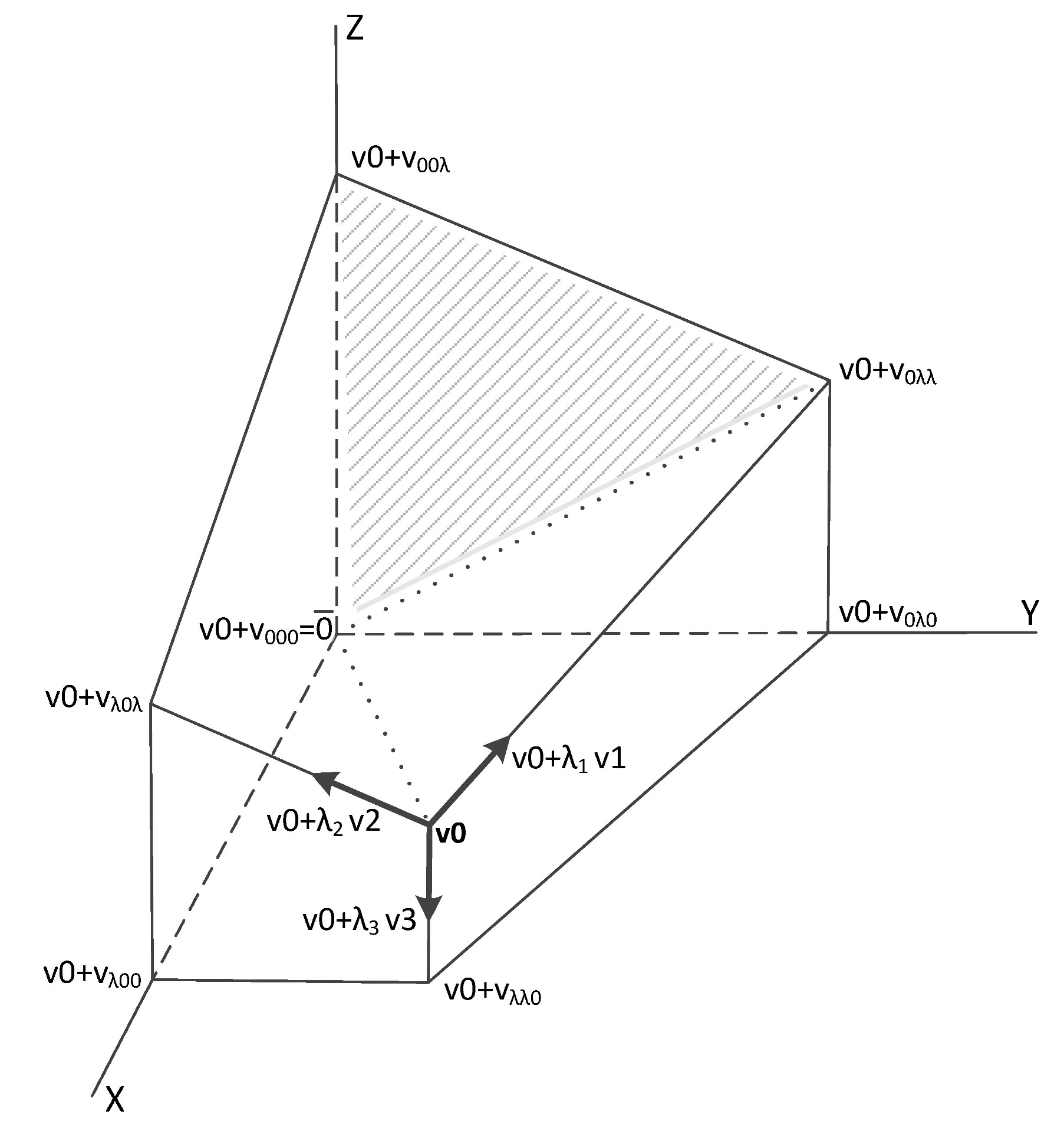
Figure 1: $3$-dimensional convex cone spanned by the three vectors $v{}_{1}$, $v{}_{2}$ and $v{}_{3}$ and cut by the planes $X=0$, $Y=0$ and $Z=0$. Any point $V$ with positive coordinates in this convex cone corresponds to a $6$-dimensional vector ${\scriptstyle\left(\begin{array}[]{c}V\\ U\end{array}\right)}$ majorized by $\left(\begin{array}[]{c}v_{0}\\ \bar{0}\end{array}\right)$.

The proof proceeds in two steps. In a first step, I decompose the convex cone $C$ into six convex cones. In each of those six convex cones, one of the plane $X=0$, $Y=0$ or $Z=0$ separates the points with nonnegative coordinates from the points that have at least one negative coordinate. In the second step, I complete the proof by showing that $v{}_{0}$ majorizes each vertices of the six convex cones cut by one of the plane $X=0$, $Y=0$ or $Z=0$.

Step1. To explain the first step, I replace the vectors $v_{1}$, $v_{2}$ and $v_{3}$ by the proportional vectors $v_{0\lambda\lambda}$, $v_{\lambda 0\lambda}$ and $v_{\lambda\lambda 0}$ respectively. The example of the vector $v_{\lambda 0\lambda}$ can be used to describe how the indices are chosen: the $0$ as second index in $v_{\lambda 0\lambda}$ indicates that the second coordinate of $v_{0}+v_{\lambda 0\lambda}$ is zero whereas the $\lambda$ as 1^st and 3^rd indices of $v_{\lambda 0\lambda}$ indicate that for this vector, $\lambda_{1}=\lambda_{3}=0$ in Eq. (111). This means that the 1^st and 3^rd coordinates of $v_{0}+v_{\lambda 0\lambda}$ are nonnegative as a direct consequence of Eq. (104). The points $v_{0}+v_{iii}$ with $i=0$ or $i=\lambda$, are illustrated in Figure 1.

Let $V$ be a given point of the convex cone C in $\mathbb{R}{}^{3}$,

$$V=v_{0}+\lambda_{1}^{\prime}v_{0\lambda\lambda}+\lambda_{2}^{\prime}v_{\lambda 0\lambda}+\lambda_{3}^{\prime}v_{\lambda\lambda 0},\qquad\lambda_{k}^{\prime}\geqslant 0.$$ (119)

As can be visualized in Figure 1 and checked in Table 1, the vector $\bar{0}=v_{0}+v_{000}$ is within the convex cone $C$ and can be used to decompose it into three convex cones. I assume without loss of generality that $V$ is in the convex cone $C_{3}$ defined by the three vectors $v_{0\lambda\lambda}$, $v_{\lambda 0\lambda}$ and $v_{000}$,

$$V=v_{0}+\lambda_{1}^{\prime\prime}v_{0\lambda\lambda}+\lambda_{2}^{\prime\prime}v_{\lambda 0\lambda}+\lambda_{3}^{\prime\prime}v_{000},\qquad\lambda_{k}^{\prime\prime}\geqslant 0.$$ (120)

I further decompose the convex cone $C_{3}$ by introducing the linear combination of the first two vectors that span the cone, $v_{00\lambda}=\mu_{1}v_{0\lambda\lambda}+\mu_{2}v_{\lambda 0\lambda}$, where the two first coordinates of $v_{0}+v_{00\lambda}$ equal to zero and, for this vector, $\lambda_{3}=0$ in Eq. (111). It will be clear in Table 1 that the vector $v_{0}+v_{00\lambda}$ is within the convex cone $C_{3}$ (both $\mu_{1}$ and $\mu_{2}$ are nonnegative) and can be used to decompose $C_{3}$ into two convex cones. I assume without loss of generality that the vector $v_{\lambda 0\lambda}$ can be replaced in Eq. (120) so that $V$ is in the convex cone $C{}_{31}$ defined as

$$V=v_{0}+\lambda_{1}^{\prime\prime\prime}v_{0\lambda\lambda}+\lambda_{2}^{\prime\prime\prime}v_{00\lambda}+\lambda_{3}^{\prime\prime}v_{000},\qquad\lambda_{k}^{\prime\prime\prime}\geqslant 0.$$ (121)

In summary, the initial convex cone $C$ can be decomposed into six convex cones. The initial convex cone $C$ is the union of the six convex cones and any point of the convex cone $C$ can be retrieved in one of the six convex cones. Each of the six convex cones has properties similar to $C{}_{31}$:

• The convex cone $C{}_{31}$ is defined by the three vectors $v_{0\lambda\lambda}$, $v_{00\lambda}$ and $v_{000}$, denoted below by $v_{0ii}$ where $i=0$ or $i=\lambda$;

• by construction, each of the three vectors $v_{0}+v_{0ii}$ has the first coordinate $X=0$ and a nonnegative value for the two other coordinates;

• as a consequence, within the convex cone $C{}_{31}$, the plane $X=0$ separates the points that have all nonnegative coordinates from the points that have at least the first coordinate $X<0$. The hatched area in Figure 1 illustrates this separation for the convex cone $C{}_{31}$.

Step 2. The second step of the proof consists in proving that the vertices of the six convex cones limited by one of the plane $X=0$, $Y=0$ or $Z=0$ correspond to vectors ${\scriptstyle\left(\begin{array}[]{c}V\\ U\end{array}\right)}$ that are all majorized by $v{}_{0}$.

Table 1 shows the coordinates of each of the points $v_{0}+v_{iii}$ in $\mathbb{R}{}^{3}$, the corresponding values $\lambda_{1}$, $\lambda_{2}$ and $\lambda_{3}$ as well as the corresponding vectors ${\scriptstyle\left(\begin{array}[]{c}V\\ U\end{array}\right)}$ in $\mathbb{R}{}^{6}$.

$v_{0}+v_{iii}$	$V^{\intercal}$	$\left(V^{\intercal},U^{\intercal}\right)$	$\lambda{}_{1}$	$\lambda{}_{2}$	$\lambda{}_{3}$
$v{}_{0}$	$\left(a^{0},a^{1},a^{2}\right)$	$\left(a^{0},a^{1},a^{2},0,0,0\right)$	$0$	$0$	$0$
$v{}_{0}+v_{000}$	$\left(0,0,0\right)$	$\left(0,0,0,a^{0},a^{1},a^{2}\right)$	$1$	$1$	$1$
$v{}_{0}+v_{0\lambda\lambda}$	$\left(0,a^{0},a^{1}\right)$	$\left(0,a^{0},a^{1},a^{2},0,0\right)$	$1$	$0$	$0$
$v{}_{0}+v_{\lambda 0\lambda}$	$\left(a^{0},0,a^{1}\right)$	$\left(a^{0},0,a^{1},a^{2}-a^{3},a^{3},0\right)$	$0$	$a{}^{1}$	$0$
$v{}_{0}+v_{\lambda\lambda 0}$	$\left(a^{0},a^{1},0\right)$	$\left(a^{0},a^{1},0,a^{2}-a^{3},a^{3}-a^{4},a^{4}\right)$	$0$	$0$	$a^{2}$
$v{}_{0}+v_{\lambda 00}$	$\left(a^{0},0,0\right)$	$\left(a^{0},0,0,a^{1}-a^{3},a^{2},a^{3}\right)$	$0$	$a^{1}$	$a^{1}$
$v{}_{0}+v_{0\lambda 0}$	$\left(0,a^{0},0\right)$	$\left(0,a^{0},0,a^{1},a^{2}-a^{3},a^{3}\right)$	$1$	$0$	$a^{1}$
$v{}_{0}+v_{00\lambda}$	$\left(0,0,a^{0}\right)$	$\left(0,0,a^{0},a^{1},a^{2},0\right)$	$1$	$1$	$0$

Table 1: Values of $V^{\intercal}$ and corresponding $\left(V^{\intercal},U^{\intercal}\right)$ for the vertices of the polytope defined by the convex cone $C$ cut by the planes $X=0$, $Y=0$ and $Z=0$.

It is directly apparent in Table 1 that the eight vectors ${\scriptstyle\left(\begin{array}[]{c}V\\ U\end{array}\right)}$ are majorized by the first vector $\left(\begin{array}[]{c}v_{0}\\ \bar{0}\end{array}\right)$. The first vector $\left(\begin{array}[]{c}v_{0}\\ \bar{0}\end{array}\right)$ indeed majorizes itself and each other vector ${\scriptstyle\left(\begin{array}[]{c}V\\ U\end{array}\right)}$ may be obtained from $\left(\begin{array}[]{c}v_{0}\\ \bar{0}\end{array}\right)$ by performing Robin Hood transfers.

The convexity property mentioned earlier completes the proof of the theorem in the case $N=3$.

The following three observations remain valid for any value $N$.

• a majorized vector ${\scriptstyle\left(\begin{array}[]{c}V\\ U\end{array}\right)}$ can be the convolution of $v_{0}$ with a vector that has negative elements. As an example, the point $v_{0}+v_{\lambda 0\lambda}$ corresponds to the convolution of $\left(a^{0},-a^{1},a^{1}\right)^{\intercal}$ with $v_{0}$;

• a majorized vector ${\scriptstyle\left(\begin{array}[]{c}V\\ U\end{array}\right)}$ can correspond to the convex combination of vectors of the convex cone $C$ that have negative elements. As an example, the point $v_{0}+v_{00\lambda}$ is the convex combination with equal weights of $v_{0}+2v_{1}$ and $v_{0}+2v_{2}$ that both contain negative elements;

• it is not necessary for the convolution to have the form specified by Eq. (111) to get a vector majorized by $v{}_{0}$. As an example, the convolution with $\lambda_{1}=a$, $\lambda_{2}=-\epsilon$ and $\lambda_{3}=a^{2}$ with $0<\epsilon\leqslant\left(1-a\right)^{2}$ defines a point outside of the convex cone $C$ that corresponds to a vector ${\scriptstyle\left(\begin{array}[]{c}V\\ U\end{array}\right)}$ majorized by $v{}_{0}$.

The same two steps of the proof for $N=3$ directly generalize to other values for $N$.

Step 1. The step by step decomposition of the convex cone generalizes in the $N$-dimensional space into a decomposition that will end up with $N!$ convex subcones.

A point of the initial convex cone $C$ is defined as

$$V =v_{0}+\lambda_{1}v_{1}\hskip 16.06pt+\lambda_{2}v_{2}\hskip 22.08249pt+\dots+\lambda_{N-1}v_{N-1}\hskip 7.02625pt+\lambda_{N}v_{N},\hskip 34.12749pt\lambda_{k}\geqslant 0,$$ (122a)

$$=v_{0}+\lambda_{1}^{\prime}v_{0\lambda\dots\lambda}+\lambda_{2}^{\prime}v_{\lambda 0\lambda\dots\lambda}+\dots+\lambda_{N-1}^{\prime}v_{\lambda\dots\lambda 0\lambda}+\lambda_{N}^{\prime}v_{\lambda\dots\lambda 0},\qquad\lambda_{k}^{\prime}\geqslant 0,$$ (122b)

where, in Eq. (122b), the $N$ indices uniquely define each vector $v_{i_{1}i_{2}\dots i_{N}}$ and are chosen as in the case $N=3$: an index $i_{k}=0$ indicates that the $k$-th coordinate of $v_{0}+v_{i_{1}i_{2}\dots i_{N}}$ is zero and an index $i_{k}=\lambda$ indicates that $\lambda_{k}=0$ when this vector is expressed in the initial convex cone defined by Eq. (111).

It will be shown in Step 2 that all vectors $v_{0}+v_{i_{1}i_{2}\dots i_{N}}$, with any combination of the indices, are inside the convex cone $C$. This property, added to the fact that the $N$ vectors $v_{k}$ are linearly independent, allows us to express any vector of the initial convex cone as a vector of one of the $N!$ subcones that has, without loss of generality, the following form:

$$V=v_{0}+\lambda_{1}^{\prime\prime}v_{0\lambda\dots\lambda}+\lambda_{2}^{\prime\prime}v_{00\lambda\dots\lambda}+\dots+\lambda_{N-1}^{\prime\prime}v_{0\dots 0\lambda}+\lambda_{N}^{\prime\prime}v_{0\dots 0},\qquad\lambda_{k}^{\prime\prime}\geqslant 0,$$ (123)

where the first vector has one index $i_{1}=0$, the second vector has two indices $i_{1}=i_{2}=0$, up to the last vector with $N$ zero indices $v_{0\dots 0}$.

Similarly to the $N=3$ case, the following statements apply to the $N!$ convex subcones (the indices and coordinates must be permuted to describe properly each subcone):

• The $N$-dimensional convex subcone is defined by its vertex $v{}_{0}$ and by the $N$ vectors $v_{0\lambda\dots\lambda}$,…, $v_{0\dots 0\lambda}$ and $v_{0\dots 0}$;

• the $N$ vectors $v_{0}+v_{0\lambda\dots\lambda}$,…, $v_{0}+v_{0\dots 0\lambda}$ and $v_{0}+v_{0\dots 0}$ have a first coordinate $X_{1}=0$ and a nonnegative value for the other coordinates;

• as a consequence and by linearity, within the convex subcone defined by the $N$ vectors $v_{0\lambda\dots\lambda}$,…, $v_{0\dots 0\lambda}$ and $v_{0\dots 0}$, the hyperplane $X_{1}=0$ separate the points that have all nonnegative coordinates from the points that have at least the first coordinate $X_{1}<0$.

Step 2. Because the initial convex cone $C$ is the union of $N!$ convex subcones similar to the subcone defined by Eq. (123), it must be proved that the vectors $v_{0}+v_{i_{1}i_{2}\dots i_{N}}$ with all possible combinations of the indices $i_{k}=0$ or $i_{k}=\lambda$ correspond to $2N$-dimensional vectors ${\scriptstyle\left(\begin{array}[]{c}V\\ U\end{array}\right)}$ that are majorized by $v{}_{0}$.

I use a step by step procedure to construct the points $v_{0}+v_{i_{1}i_{2}\dots i_{N}}$ of the convex cone $C$ such that either $i_{k}=0$ or $i_{k}=\lambda$, starting from the lowest index.

Let us assume that the $j$-th element is the first (lowest index) zero of a given vector $v_{0}+v_{i_{1}i_{2}\dots i_{N}}$: $i{}_{j}=0$ and $i_{1}=\dots=i_{j-1}=\lambda$. We can observe in Eq. (104) that any vector $v_{k}$ has only one negative element, its $k$-th element, whose value is $-a^{0}=-1$.

The initial value of the $j$-th element of $v{}_{0}$ is $a^{j-1}$ and - within the convex cone $C$ - a zero can only be obtained by adding a vector $a^{j-1}v_{j}$ to $v_{0}$. Using Eq. (104), the effects of adding $a^{j-1}$$\left(\begin{array}[]{c}v_{j}\\ u_{j}\end{array}\right)$ to $\left(\begin{array}[]{c}v_{0}\\ \bar{0}\end{array}\right)$ can be described as follows:

• The first $j-1$ elements of $V$ are unchanged and keep their values $a^{0},a^{1},\dots,a^{j-2}$;

• the $j$-th element of $V$ decreases from the value $a^{j-1}$ to $0$; we can consider that this element decreases by slices, that is, first from $a^{j-1}$ to $a^{j}$, then from $a^{j}$ to $a^{j+1}$, and so on, until the $N$-th slice, from $a^{N+j-2}$ to $0$;

• the decrease in value of the $j$-th element of $V$ is compensated by increases of the values of the $N$-th subsequent elements of ${\scriptstyle\left(\begin{array}[]{c}V\\ U\end{array}\right)}$: the $j+1$-th element is increased by the first slice, that is, from $a^{j}$ to $a^{j-1}$, the next element is increased by the second slice from $a^{j+1}$ to $a^{j}$ and so on. Those transfers within the $V$ part of ${\scriptstyle\left(\begin{array}[]{c}V\\ U\end{array}\right)}$ are all Robin Hood transfers;

• after the transfers to the $V$ part of ${\scriptstyle\left(\begin{array}[]{c}V\\ U\end{array}\right)}$ are completed, the subsequent slices are transferred to the $U$ part of ${\scriptstyle\left(\begin{array}[]{c}V\\ U\end{array}\right)}$. Before these transfers, all the elements of $U$ had a zero value, which means that all the transfers from the $j$-th element of $V$ to the $U$ part of ${\scriptstyle\left(\begin{array}[]{c}V\\ U\end{array}\right)}$ are also Robin Hood transfers;

• after this first step, the $N$ elements of ${\scriptstyle\left(\begin{array}[]{c}V\\ U\end{array}\right)}$ that have been increased ($j+1$-th to $j+N$-th) have the form $a^{i}$ or $a^{i}-a^{i+p}$ where $p$ is a positive integer and where the exponent $i$ increases continuously from element to element, by steps equal to $1$.

The effect of adding an additional vector $a^{j^{\prime}-2}$$\left(\begin{array}[]{c}v_{j^{\prime}}\\ u_{j^{\prime}}\end{array}\right)$ to the obtained vector can be sliced into Robin Hood transfers in the same way as for the first vector. After each addition, the vector ${\scriptstyle\left(\begin{array}[]{c}V\\ U\end{array}\right)}$ keeps the same structure and in particular, the elements that follow the element that has just been put to zero keep the same structure $a^{i}$ or $a^{i}-a^{i+p}$ where $p$ is a positive integer and where the exponent $i$ increases from element to element, by steps equal to $1$.

Two steps of this procedure are illustrated in Table 2 to construct the vector $v_{0}+v_{\lambda\lambda 0\lambda\lambda 0\lambda}$ in the case $N=7$, first for $j=3$ and then for $j^{\prime}=6$.

$$\begin{array}[]{ccccc}\begin{array}[]{c}v_{0}+v_{\lambda\lambda\lambda\lambda\lambda\lambda\lambda}\end{array}&\longrightarrow&v_{0}+v_{\lambda\lambda 0\lambda\lambda\lambda\lambda}&\longrightarrow&v_{0}+v_{\lambda\lambda 0\lambda\lambda 0\lambda}\\ \\ \\ \left(\begin{array}[]{c}v_{0}\\ \bar{0}\end{array}\right)&\longrightarrow&\left(\begin{array}[]{c}v_{0}\\ \bar{0}\end{array}\right)+a^{2}\left(\begin{array}[]{c}v_{3}\\ u_{3}\end{array}\right)&\longrightarrow&\left(\begin{array}[]{c}v_{0}\\ \bar{0}\end{array}\right)+a^{2}\left(\begin{array}[]{c}v_{3}\\ u_{3}\end{array}\right)+a^{4}\left(\begin{array}[]{c}v_{6}\\ u_{6}\end{array}\right)\\ \\ \\ \left(\begin{array}[]{c}\\ a{}^{0}\\ a{}^{1}\\ a{}^{2}\\ a{}^{3}\\ a{}^{4}\\ a{}^{5}\\ a{}^{6}\\ 0\\ 0\\ 0\\ 0\\ 0\\ 0\\ 0\\ \\ \end{array}\right)&\longrightarrow&\left(\begin{array}[]{ccc}\\ &a{}^{0}\\ &a{}^{1}\\ &0\\ &a{}^{2}\\ &a{}^{3}\\ &a{}^{4}\\ &a{}^{5}\\ &a^{6}-a^{7}\\ &a^{7}-a^{8}\\ &a^{8}\\ &0\\ &0\\ &0\\ &0\\ \\ \end{array}\right)&\longrightarrow&\left(\begin{array}[]{ccc}\\ &a{}^{0}\\ &a{}^{1}\\ &0\\ &a{}^{2}\\ &a{}^{3}\\ &0\\ &a{}^{4}\\ &a^{5}-a^{7}\\ &a^{6}-a^{8}\\ &a^{7}\\ &a^{8}-a^{9}\\ &a^{9}-a^{10}\\ &a^{10}\\ &0\\ \\ \end{array}\right)\end{array}$$

Table 2: Illustration of the two successive steps to construct the vector $v_{0}+v_{\lambda\lambda 0\lambda\lambda 0\lambda}$ in the case $N=7$. It is clear that $v{}_{0}$ majorizes the vector ${\scriptstyle\left(\begin{array}[]{c}V\\ U\end{array}\right)}$ corresponding to $v_{0}+v_{\lambda\lambda 0\lambda\lambda\lambda\lambda}$, which in turn majorizes the vector ${\scriptstyle\left(\begin{array}[]{c}V\\ U\end{array}\right)}$ corresponding to $v_{0}+v_{\lambda\lambda 0\lambda\lambda 0\lambda}$.

The construction described above demonstrates how a vector $v_{0}+v_{i_{1}i_{2}\dots i_{N}}$ with any combination of the indices $i_{k}=0$ or $i_{k}=\lambda$, can be obtained from the initial vector $\left(\begin{array}[]{c}v_{0}\\ \bar{0}\end{array}\right)$ by successively adding vectors $\lambda_{k}$$\left(\begin{array}[]{c}v_{k}\\ u_{k}\end{array}\right)$ for each position $k$ where the index $i_{k}=0$ in $v_{0}+v_{i_{1}i_{2}\dots i_{N}}$. Each addition of vector $\lambda_{k}$$\left(\begin{array}[]{c}v_{k}\\ u_{k}\end{array}\right)$ - with $\lambda{}_{k}$ properly chosen - can be decomposed into Robin Hood transfers. Consequently, the vector $\left(\begin{array}[]{c}v_{0}\\ \bar{0}\end{array}\right)$ majorizes all vectors ${\scriptstyle\left(\begin{array}[]{c}V\\ U\end{array}\right)}$ constructed in this manner. This completes the proof of Theorem 1.

Proof of Theorem 2

I outline (only) the main steps of the extension of Theorem 1 to the continuous case. My approach consists in showing that the continuous convolution of Theorem 2 can be obtained as the limit of a sequence of vectors that match the entry criteria of Theorem 1.

Let $c(z)$ be the function defined in the statement of Theorem 2 in section 3.

I define an interval $\left[z_{0},z_{end}\right]$ on the positive real axis with $z_{0}=0$ and I partition that interval into $2N$ equal sub-intervals such that $z{}_{i}-z_{i-1}=\Delta z,\>i=1,\dots,2N$. Within the first $N$ sub-intervals $\left[z_{i-1},z{}_{i}\right],\>i=1,\dots,N,$ I choose $z_{i}^{\prime}$ so that $c\left(z_{i}^{\prime}\right)$ is the supremum of the function $c\left(z\right)$ on that sub-interval.

I construct a $N+1$-dimensional vector $C_{N+1}$ that fulfills (for $\Delta z$ sufficiently small) the condition specified by Eq. (52):

$$C{}_{N+1}=\tilde{k}_{N+1}\left(\begin{array}[]{c}c_{\delta 0}\\ \overset{\vphantom{10}}{c\left(z_{1}^{\prime}\right)\left(1-e^{-\Delta z}\right)}\\ \vdots\\ c\left(z_{N-1}^{\prime}\right)\left(1-e^{-\Delta z}\right)\\ \overset{\vphantom{10}}{c_{last}\frac{\left(1-e^{-\Delta z}\right)}{\Delta z}}\end{array}\right),$$ (129)

where $c_{\delta 0}$ is the factor multiplying the Dirac delta function of $c(z)$ in $z=0$ , $\tilde{k}_{N+1}$ ensures that the vector $C{}_{N+1}$ is normalized and

$$c_{last}=\intop_{z_{N}}^{+\infty}\;c\left(z\right)\;\mathrm{d}z.$$ (130)

I also define the $N$-dimensional vector $e{}_{0}=\left(e^{-0\Delta z},e^{-1\Delta z},e^{-2\Delta z},\dots,e^{-\left(N-1\right)\Delta z}\right)^{\intercal}$.

It can be seen that the discrete convolution $G_{2N}=C_{N+1}*e_{0}$ is nonnegative by decomposing the continuous convolution $g\left(z\right)=c\left(z\right)\ast e^{-z}$ into a discrete sum. It is calculated at one of the points that define the first $N-1$ sub-intervals, $z=z_{j}$ as follows

$$g\left(z_{j}\right) =\sum_{i=1}^{j}\;\intop_{z_{i-1}}^{z_{i}}c\left(x\right)e^{-\left(z_{j}-x\right)}\mathrm{d}x$$ (131a)

$$=c_{\delta 0}\>e^{-z_{j}}+\sum_{i=1}^{j}\;c\left(z_{i}^{\prime\prime}\right)\;\intop_{z_{i-1}}^{z_{i}}e^{-\left(z_{j}-x\right)}\mathrm{d}x$$ (131b)

$$=c_{\delta 0}\>e^{-z_{j}}+\left(1-e^{-\Delta z}\right)\;\sum_{i=1}^{j}\;c\left(z_{i}^{\prime\prime}\right)\;e^{-\left(z_{j}-z_{i}\right)},$$ (131c)

where the points $z_{i}^{\prime\prime}$ within each sub-intervals are determined by the mean value theorem.

The points $z_{i}^{\prime}$ were chosen so that $c\left(z_{i}^{\prime}\right)\geqslant c\left(z_{i}^{\prime\prime}\right),\>i=1,\dots,N$. The sum in Eq. (131c) has the same form as the discrete convolution $G_{2N}$ and it shows that if the continuous convolution $g\left(z_{j}\right)$ is nonnegative, then the $j+1$-th element of the discrete convolution $G_{2N}$ is nonnegative - also at the points where the continuous convolution $g\left(z\right)$ might have a zero value.

A second variable name $y$ is associated with the index $j$ and the $j+1$-th element of the discrete convolution $G_{2N}=C_{N+1}*e_{0}$ is denoted $G_{2N}\left(y_{j}\right),\>j=0,\dots,2N-1$.

The three vectors $C_{N+1}$, $e_{0}$ and $G_{2N}$ are within the conditions of Theorem 1 for any sufficiently small value of $\Delta z$ as well as for any choice of $z_{end}$ that defines the initial interval.

Because in this case $e_{0}\;\succ G_{2N}$, Eq. (3) can be used to write the $2N$ equations

$$G_{2N}\left(y_{j}\right)=\sum_{i=0}^{N-1}D_{2N}\left(z_{i,},y_{j}\right)\;e^{-z_{i}},\qquad j=0,\dots,2N-1,$$ (132)

where $0\leqslant D_{2N}\left(z_{i,},y_{j}\right)\leqslant 1$ are the elements of a $2N\times 2N$ doubly stochastic matrix.

As $\Delta z$ tends to zero, $N$ to infinity and $z_{end}$ to infinity,

• the vector $G_{2N}$ tends to the continuous convolution $g\left(z\right)$ of the distribution $e{}^{-z}$ with the function $c\left(z\right)$ (both are integrable functions and improper integrals are absolutely convergent);

• the sum in Eq. (132) takes the form of a convergent Riemann–Stieltjes integral whose integrand is $e{}^{-z}$ and whose integrator function is monotone and of bounded variation (this integrator function could be a generalized function).

At the limit, the sum in Eq. (132) identifies with the condition for continuous majorization set out in Eq. (7). This completes the proof of Theorem 2.

5 Conclusion

I have proved that the nonnegative Wigner function of any mixture of Fock states is majorized by the Wigner function of the vacuum.

The fact that the Wigner function results from a convolution is revealed to be a decisive factor in this majorization relation. I have described the underlying new majorization property dedicated to convolutions with the negative exponential distribution.

As a corollary to the majorization relation, the Shannon differential entropy of the Wigner function of the vacuum is lower than the entropy of the Wigner function of any mixture of Fock states. This same order between the Wigner functions of the vacuum and any mixture of Fock states is also respected for any other entropy, provided that the latter is defined by a concave function.

I conjecture that properties similar to the ones described in this article may explain further majorization relations between the Wigner function of the vacuum and other states than mixtures of Fock states - after all, any Wigner function can be obtained as a convolution of the Sudarshan-Glauber P representation.

References

- [1] J. Weinbub and D. K. Ferry. Recent advances in wigner function approaches. Applied Physics Reviews, 5(4):041104, 2018.
- [2] Ivan V. Bazarov. Synchrotron radiation representation in phase space. Phys. Rev. ST Accel. Beams, 15:050703, May 2012.
- [3] Anatole Kenfack and Karol yczkowski. Negativity of the wigner function as an indicator of non-classicality. Journal of Optics B: Quantum and Semiclassical Optics, 6(10):396–404, aug 2004.
- [4] Iwo Białynicki-Birula and Jerzy Mycielski. Uncertainty relations for information entropy in wave mechanics. Communications in Mathematical Physics, 44(2):129–132, 1975.
- [5] Anaelle Hertz, Michael G Jabbour, and Nicolas J Cerf. Entropy-power uncertainty relations: towards a tight inequality for all gaussian pure states. Journal of Physics A: Mathematical and Theoretical, 50(38):385301, 2017.
- [6] Raymond J. Hickey. Majorisation, randomness and some discrete distributions. Journal of Applied Probability, 20(4):897–902, 1983.
- [7] Barry C Marshall Albert W;Olkin Ingram;Arnold. Inequalities : Theory of Majorization and Its Applications. Springer, New York, 2010.
- [8] Raymond J. Hickey. Continuous majorisation and randomness. Journal of Applied Probability, 21(4):924–929, 1984.
- [9] Ulf Leonhardt. Essential Quantum Optics: From Quantum Measurements to Black Holes. Cambridge University Press, 2010.
- [10] Zacharie Van Herstraeten and Nicolas J. Cerf. Quantum wigner entropy, 2021.
- [11] Michael A. Nielsen and Isaac L. Chuang. Quantum Computation and Quantum Information (Cambridge Series on Information and the Natural Sciences). Cambridge University Press, 1 edition, January 2004.
- [12] Peter Day. Decreasing rearrangements and doubly stochastic operators. Transactions of The American Mathematical Society, 178:383–383, 04 1973.
- [13] Harry Joe. An ordering of dependence for distribution of k-tuples, with applications to lotto games. Canadian Journal of Statistics, 15(3):227–238, 1987.