∎
Tel.: +49 (0)231 755 3231
Fax: +49 (0)231 755 5416
22email: michael.sievers@math.tu-dortmund.de
Convergence Analysis of a Local Stationarity Scheme for Rate-Independent Systems and Application to Damage††thanks: This research was supported by the German Research Foundation (DFG) under grant number KN 1131/3-1 within the priority program Non-smooth and Complementarity-based Distributed Parameter Systems: Simulation and Hierarchical Optimization (SPP 1962).
Abstract
This paper is concerned with an approximation scheme for rate-independent systems governed by a non-smooth dissipation and a possibly non-convex energy functional. The scheme is based on the local minimization scheme introduced in EM (06), but relies on local stationarity of the underlying minimization problem. Under the assumption of Mosco-convergence for the dissipation functional, we show that accumulation points exist and are so-called parametrized solutions of the rate-independent system. In particular, this guarantees the existence of parametrized solutions for a rather general setting. Afterwards, we apply the scheme to a model for the evolution of damage.
Keywords:
Rate independent evolutions parametrized solutions unbounded dissipation existence finite elements semi-smooth Newton methods damage1 Introduction
The effect of rate-independence occurs in various different areas of mechanics. This concerncs for example the field of elastoplasticity, damage and shape-memory, to only mention a few (see, e.g., KRZ (13); FM (06); Mai (04); AMS (08); MM (09)). One main characteristic of such systems is the fact that changes in the state are solely driven by an external force. What is more, as the name already suggests, the system is independent of the rate at which the loading is applied, that is to say, whenever is a solution to some external load , then is a solution to for every monotone increasing function .
In this paper we consider rate-independent systems that can be described by the following differential inclusion
| (RIS) |
One may see this inclusion as a balance of forces, i.e. the dissipative force and the potential force must annihilate each other. Implicitly hidden within this formulation is the fact that the potential force as well as the dissipative force result from a (possibly non-convex) energy functional and a dissipation functional . While we postpone the exact assumptions to Section 2, let us mention at this point that the characteristic feature of the formulation in (RIS) is the positive -homogeneity of the dissipation . It is this property which induces that (RIS) is indeed rate-independent. However, the combination of non-convex energies and positive -homogeneous dissipations allow the formation of abrupt changes in the state, even if the external forces evolve smoothly. Hence, suitable notions of solutions for (RIS) need to be able to handle temporal discontinuities. One such concept are the so-called parametrized solutions, whose exact definition is given in Definition 2.4. Loosely speaking, such solutions are considered as curves in the extended phase space and parametrized by arc-length. The jump path from one state to the other thus becomes an integral part of the solution itself. This idea was first applied in MMMG (94); MSGMM (95); Bon (96) for systems with dry friction and later on generalized in EM (06) and MRS (09); MZ (14) for finite and infinite dimensional problems, respectively. Particularly, in EM (06), the authors introduced the following time-incremental local minimization scheme for the approximation of parametrized solutions:
| (1.1a) | ||||
| (1.1b) | ||||
It was moreover shown that, for , subsequences of discrete solutions generated by (1.1) (weakly) converge to a parametrized solution. While the authors in EM (06) considered a finite dimensional setting, in Neg (14); MS (17) and particularly Kne (19) the results have been generalized to the infinite dimensional problems at least for semilinear energies. Furthermore, in MS19a the scheme was combined with a discretization in space. In this paper we extend these result to more general energy and dissipation functionals on the one side and, additionally, build the scheme upon stationary points rather then minimizer of (1.1). The actual scheme ( (LISS).) is presented in Section 3. Let us underline that the consideration of stationary points instead of (global) minimizers is of major importance from a numerical point of view, since optimization algorithms can in general only compute stationary points. What is more, we incorporate unbounded dissipations into our convergence analysis, which allows us to apply our scheme to a model for the evolution of damage.
Now, let us shortly outline the paper. In Section 2, we introduce our notation and state the assumptions on the energy and the dissipation functional. Moreover, we recall the precise notion of parametrized solutions. Section 3 is then devoted to the presentation of the actual local stationarity scheme and its convergence analysis. Particularly, since we allow the dissipation to be approximated by some functional , we provide suitably adapted a-priori estimates for the discrete solution which still meets a discrete version of an energy-equality. Building on that, we derive our main convergence result in Theorem 3.14. In Section 4, we then focus on a rate-independent damage model and describe the algorithmic realization of the discrete stationarity scheme based on a semismooth Newton-method. Finally, we present a numerical example and compare it with results from the literature.
2 Basic notations and standing assumptions
Let us start with some basic notation used throughout the paper. In the following, always stands for a generic constant. Moreover, given two normed linear spaces , we denote by the dual pairing and suppress the subscript, if there is no risk for ambiguity. By , we denote the norm in and is the space of linear and bounded operators from to . If is even a Hilbert space, we write for the Riesz isomorphism. Furthermore, is the open ball in around with radius . Given a convex functional , we denote the (convex) subdifferential of at by and its conjugate functional by . Finally, stands for the Lebesgue measure of a set , and describes the set of vectors in whose components are greater or equal to .
2.1 Assumptions on the data
Let us now introduce the assumptions on the quantities in (RIS). We assume that the underlying spaces and are Banach spaces with . Moreover, and are required to be reflexive and separable.
Energy
The energy is supposed to fulfill:
- (E1)
-
.
- (E2)
-
For all the energy is weakly lower semicontinuous and coercive on with for some constants .
- (E3)
-
There exists and with such that for all :
- (E4)
-
For all sequences and in it holds:
Note that the combination of (E1)–(E3) already yields that, for all sequences and in , it holds
| (2.1) |
Moreover, we assume that satisfies the following Gårding-like inequality:
| (2.2) |
With respect to the time component we require
| (2.3) |
Finally, we assume that is (strong,weak)-weak-continuous, i.e.,
| (2.4) |
The above assumptions combined with Gronwall’s lemma allow us to obtain the following estimates that hold for all :
| (2.5) | ||||
| (2.6) |
An energy functional that satisfies all assumptions made here is given in Section 4.
Dissipation
Regarding the dissipation , we assume that
- (R1)
-
is proper, convex and lower semicontinuous,
- (R2)
-
is positively -homogeneous, i.e., ,
- (R3)
-
.
Remark 2.1.
Note that we allow for an unbounded dissipation, which is essential for the application of our method to the damage model in Section B.
Combining the convexity and the positive -homogeneity of , it is easy to verify the following triangle inequality
| (2.7) |
In fact we allow for an approximation of the "original" dissipation in our convergence analysis. In general, this corresponds to an approximation using e.g. finite elements. However, we will keep the setting general here, that is, we assume satisfies the same assumptions as , i.e. (R1)-(R3), and Mosco-converges to w.r.t. the space in the following sense:
| (2.8a) | |||
| (2.8b) | |||
Remark 2.2.
Note that from now on, we consider and , respectively, as mapping from into . In fact, we will subsequently always evaluate at a point in . Thus, the space is not used in the convergence analysis. Moreover, the choice (i.e., no additional approximation of ) is clearly possible and fulfills all these assumptions. Another example that complies with all the assumptions (R1)-(R3) and (2.8) but satisfies is given in Section 4.2 below.
Remark 2.3.
In view of the previous Remark 2.2, for any the subdifferential is subsequently considered as a subset of , i.e., by Lemma A.1 we have iff
In particular, in order to ease notation, we will refrain from using keeping in mind that . Clearly, by the convexity and lower semicontinuity of , the set is also weakly closed in .
Initial state
The initial value is supposed to satisfy and the local stability . Moreover, we assume that the approximations of the initial value as well satisfy for all and that is bounded in independent of .
2.2 Definition of parametrized solutions
We now turn to the actual definition of the so-called parametrized solutions. As indicated in the introduction, this concept takes care of possible jump paths and relies on an energy identity.
Definition 2.4.
Let an initial value be given. We call a tuple parametrized solution of (RIS), if there exists an artificial end time such that the following conditions are satisfied:
-
(i)
Regularity:
(2.9) -
(ii)
Initial and end time condition:
(2.10) - (iii)
-
(iv)
Energy identity:
(2.12)
If, in addition to the second inequality in (2.11a), there is a constant such that f.a.a. , then the solution is called non-degenerate parametrized solution, otherwise we call it degenerate parametrized solution.
We point out that it is always possible to rescale the artificial time in order to obtain a normalized parametrized solution, where f.a.a. . The key idea here is to cut out all intervals where and to scale the artificial time appropriately, see, e.g., (Sie, 20, Lem. A.4.3). Moreover, let us mention that the regularity conditions in our definition of parametrized solutions are chosen in such a way, that all terms contained are well-defined. Depending on the actual setting, particularly the choice of and , there might exist slightly different requirements, see, e.g., (MRS, 16, Def. 4.2).
3 Local stationarity scheme
The ultimate goal of this section is to prove that the subsequent algorithm, which is based on the local incremental minimization scheme (1.1), provides an approximation scheme for parametrized solutions. The difference compared to (1.1) is that we search for stationary points of the constrained problem rather than global minima, see (alg1). Thus, for a given time-discretization parameter , the algorithm reads as follows:
Algorithm (LISS).
| (alg1) |
| (alg2) |
| (alg3) |
Note that merely for technical reasons, we do not use the "" from (1.1b) in the time-update. In addition, the notation is used here only once more to highlight that the subdifferential is in fact calculated in terms of the space , see also Remark 2.3. The proposed method is closely related to (1.1), since a local minimizer of
| (3.1) |
necessarily satisfies (alg1). Moreover, thanks to the assumptions on and , in particular weak lower semicontinuity, the existence of a global minimum of (3.1) and therefore also the existence of a stationary point fulfilling (alg2) is guaranteed by the direct method in the calculus of variations. The reason for investigating ( (LISS).) instead of (1.1), is the fact that a numerical algorithm for solving (1.1a) or rather (3.1) naturally provides a stationary point that satisfies but, in case of a nonconvex energy, is not guaranteed to be a global optimum of (1.1a) and (3.1), respectively. Moreover, since the concept of parametrized solutions is based on a local stability condition, it is consistent to look for locally stable points, which are exactly the stationary points of (1.1a). Despite its necessity for the convergence analysis, the inequality in (alg2) is also physically meaningful since it enforces the system to look for energetically preferable states, i.e., states with a lower energy cost. Concerning the exploration of this algorithm, particularly with a view to convergence, we proceed as follows: We start with characterizing properties of the stationary points. Afterwards, we turn to the essential a priori estimates that will allow a passage to the limit in the discrete version of the energy identity in (2.12), which is deduced in Lemma 3.10. The limit procedure itself is elaborated in the final Section 3.4.
3.1 Approximate discrete parameterized solution
The foundation for both, the a priori estimates and the discrete version of the energy identity, is given by the following Lemma 3.1. It provides various properties of a stationary point in (alg1) and shows some similarities with the complementarity in (2.11). Indeed, we will see that one can interpret the stationarity condition as a discrete version of (2.11).
Lemma 3.1 (Discrete optimality System).
Proof.
The proof is given, e.g., in MS19a ; Sie (20) under a slightly different setting. For convenience of the reader, we thus repeat the main steps. To shorten the notation we also set , cf. (A.3), and suppress the superscripts for the iterates throughout the proof. Thanks to a classical result of convex analysis, (alg1) is equivalent to
| (3.3) | ||||
Since we have
| (3.4) |
Moreover, from Lemma A.2, we infer
Inserting this together with (3.4) in (3.3) gives (3.2c).
To prove (3.2a), we consider (alg1) once more.
Since and is continuous in , the sum rule for convex
subdifferentials is applicable giving the existence of a , such that
| (3.5) |
and thereby
A comparison with (3.2c), shows that
| (3.6) | ||||
Now, the fact that , and the characterization in Lemma A.3 immediately yields (3.2a). Next, we verify (3.2b). For this purpose, we observe that by assumption is also convex and positively -homogeneous so that Lemma A.1 implies . The characterization of the conjugate functional from Lemma A.1 in combination with (3.5) thus yields
| (3.7) | ||||
| (3.8) |
Inserting this into (3.6) we arrive at (3.2b). Finally, (3.2d) is an immediate consequence of (3.7).
∎
Remark 3.2.
In fact, since (alg1) is equivalent to the properties (3.2a)–(3.2d) it might be practical to exploit the characterization via (3.2a)–(3.2d) for the actual numerical realization of ( (LISS).) instead of (alg1) in order to calculate a stationary point. Moreover, we will solely build upon this discrete optimality system (and the inequality (alg2)) for the convergence analysis.
Let us take a further look at (3.2d). Exploiting the properties of from (A.6) it is easy to see that . Inserting this into (3.2d) we find that
Combining this with (3.2a) and the time-update from (alg3) we therefore obtain
| (3.9) |
which is a discrete version of the complementarity condition in the definition of parametrized solutions, cf. (2.11).
3.2 A-priori estimates
Based on the previous Lemma 3.1, we subsequently provide several a priori estimates that will allow a passage to the limit in the discrete energy identity in Section 3.3 and 3.4, respectively. Furthermore, we show that the discrete physical time given the time update in (alg3) reaches the final time in a finite number of iterations, see Proposition 3.7 below. We start with the following collection of results, whose proofs are basic so that we refer to MS19a ; Kne (19) here. Let us, nevertheless, remark that these a priori estimates are the only point where one needs to exploit that is energetically preferred, that means (alg2) holds, and not only a stationary point satisfying (3.2a)-(3.2d).
Lemma 3.3 (Boundedness for energy and dissipation).
Proof.
Remark 3.4.
As a consequence of Lemma 3.3 and the boundedness of by assumption we have that for some independent of and .
The estimate (3.11) will, on the one hand, provide us with a uniform -bound for the linear interpolants and, on the other hand, allows us to obtain a bound for the derivative . In preparation for that, we derive the following:
Lemma 3.5.
For every , there exists , such that
| (3.12) |
for all and .
Proof.
According to Ehrling’s lemma, for every , there exists a constant such that
| (3.13) |
Combining the Garding-like inequality from (2.2) with (2.3) we find
| (3.14) |
To proceed, we consider each of the two last terms separately. For the first one, we exploit (3.13) for (recall that denotes the embedding constant of ) to obtain
| (3.15) | ||||
where we used the lower bound for from (R3) and the embedding in the last line. Next, we turn to the last term in (3.14). For this, we take advantage of Young’s inequality which gives
| (3.16) |
Inserting (3.15) and (3.16) in (3.14) we eventually arrive at (3.12).
∎
Clearly, from the uniform boundedness of the iterates and we can conclude the following result.
Corollary 3.6.
For all iterates there exists constants such that
| (3.17) |
Proof.
One major issue in the convergence analysis for parametrized solutions concerns the boundedness of the artificial time, even in the continuous setting, see, e.g., the discussion in (MR, 15, p. 218). For the discrete counterpart, the artificial time reads . In order to bound this term, we need to estimate , which is purpose of the next proposition. Moreover, we will show that the physical end time is reached after a finite number of iterations, which guarantees that the algorithm finishes in a finite number of steps.
Proposition 3.7 (Bound on artificial time).
For every parameter there exists an index such that . Moreover, there are constants independent of such that, for all , it holds
| (3.18) | ||||
| (3.19) | ||||
| (3.20) |
Proof.
The arguments are similar to Kne (19); MS19a . However, since there are some significant differences, particularly the estimate (3.19), we present the arguments in detail. Let be arbitrary. For convenience, we again suppress the superscript throughout the proof, except for in order to avoid confusion with the initial data. We start by testing (3.2d) with to obtain
| (3.21) |
Inserting (3.2b) into (3.2c) and rewriting this identity for the index (instead of ) gives . Subtracting this from (3.21) implies
Thanks to the constraint and (A.6), that is , we have
Consequently, it holds
Now, inserting the estimate from Corollary 3.6 gives
Rearranging terms and summing up the resulting estimate with respect to , we arrive at
| (3.22) |
Thanks to (3.10) it now suffices to estimate to proof (3.19), which is shown next. To this end, we again insert (3.2b) into (3.2c) to obtain for :
Adding a zero, and rearranging terms yields
| (3.23) |
By assumption, we have which gives by the characterization in Lemma A.2, so that (3.23) implies
| (3.24) |
For the first term on the left-hand side we take advantage of the assumption in (2.2) and the boundedness of the iterates from Lemma 3.3 which results in
| (3.25) |
Hence, using again the constraint we obtain
| (3.26) |
By adding (3.26) to (3.22) and applying (3.10), we arrive at
| (3.27) | ||||
where we used that by the time update in (alg3) and for the last estimate. Clearly, by the uniform boundedness of by assumption and the continuity of , the term is also bounded independent of and , which yields that . This in turn implies
| (3.28) |
which already gives (3.19) for since by (3.2b). Moreover, (3.20) is an easy consequence of the characterization in (3.2b). Note that the constant is independent of , , and . Now, let us turn towards (3.18). From the identity (3.2b) we infer that . Moreover, thanks to the time-update it holds so that
| (3.29) |
where we used (3.28) together with the embedding as well as the fact that for the last estimate. This verifies (3.18). Finally, we show that the final time is reached after a finite number of steps. For this, we observe that by the embedding estimate (3.28) implies that is convergent, thus bounded. Summing up (alg3) from to and exploiting (3.18) we therefore obtain
Hence, there must exist a finite index , possibly depending on and , so that . Lastly, since (3.28) and (3.29) hold for every , we obtain (3.18) and (3.19), respectively. ∎
In what follows we will abbreviate the index simply by having in mind that the number of time steps always depends on and .
3.3 Discrete energy-equality
In the following section, we aim at deriving a discrete analogon to the energy identity (2.12). To this end, we introduce the piecewise affine as well as the left- and right-continuous piecewise constant interpolants associated with the iterates . As indicated in the introduction, potential discontinuities of the parametrized solution are resolved by introducing an artificial time. The physical time is accordingly interpreted as a function of the very same and jumps are characterized by the plateaus of this function. This is also reflected by the time-incremental stationarity scheme ( (LISS).), where, loosely speaking, the artificial time is divided into equidistant subintervals with step size and the approximation of the parametrized solution is implicitly defined through the optimization in ( (LISS).). To be more precise, we set , so that
| (3.30) | ||||
by Proposition 3.7 with a constant which is neither depending on nor so that the artificial time interval is indeed bounded. Hence, we can proceed with the construction of the interpolants. For , the continuous and piecewise affine interpolants are defined through
| (3.31) | ||||
while the piecewise constant interpolants are given by
| (3.32) |
Moreover, we define the artificial end time as that point where reaches the end time , i.e., it holds (see also Figure 3.1)
| (3.33) |
whereby the boundedness follows directly from (3.30). Since the artificial end time depends on the chosen discretization level, we extend all interpolants constantly onto with where this is necessary, i.e., where . Hence, we let
| (3.34) |
Observe that still by (3.33). Moreover, due to the time update in (alg3), we clearly have that , but we even obtain the following pointwise properties.
Lemma 3.8 (Properties of affine interpolants).
For almost all , the affine interpolants from (3.31) fulfill
| (3.35) | |||
| (3.36) |
Proof.
The statements are a direct consequence of the properties in (3.9). ∎
Once more, we note the similarity between the continuous case in (2.11a) and (2.11b) and its discrete version in Lemma 3.8. In the subsequent, last preparatory lemma, we collect the main a priori bounds of our interpolants, which will be essential to pass to the limit in the discrete energy identity, which is elaborated afterwards.
Lemma 3.9.
There exists , independent of and , so that
Proof.
While the first three bounds are an immediate consequence of the results in Lemma 3.8 and Lemma 3.3, the last one requires some slighlty more explanation. Due to the bound in , it suffices to estimate the -norm of the time-derivative . Hence, inserting the definition of from (3.34) and keeping in mind that , we have
Lemma 3.7, precisely estimate (3.19), thus implies that this term is bounded independent of and , which proves the desired estimate. ∎
Eventually, we are now in the position to show a discrete version of the energy equality. Its proof is based on Lemma 3.8, Lemma 3.9 and the a priori estimates derived in Section 3.2.
Lemma 3.10 (Discrete energy equality).
For all , it holds
| (3.37) | ||||
where
| (3.38) |
Moreover, the complementarity condition
| (3.39) |
is fulfilled f.a.a. , and there exists a constant such that the remainder satisfies for all and all
| (3.40) |
Proof.
The complementarity in (3.39) has already been proven in Lemma 3.8. Hence, we turn to the discrete energy identity. Since the affine interpolants in (3.31) are by construction elements of and , respectively, and due to by assumption, the chain rule is applicable and gives for that
From (3.2c), we have in combination with the 1-homogeneity of that
By taking into account the definition of in (3.38),
integration over then yields (3.37).
It remains to estimate . To this end, first observe that the definition of the affine and constant interpolants in
(3.31) and (3.32) implies for every and every
that
which is frequently used in the following estimates. Now, let and be arbitrary. Then, since the Garding-like inequality from (2.2) implies
| (3.41) | ||||
Now, since we obtain from the identity in (3.38) that
for almost all . Thus (3.40) easily follows from the bounds in Lemma 3.9. ∎
Remark 3.11.
A comparison of the discrete energy identity in (3.37) and the continuous one in (2.12) shows that the coefficient is missing in front of the distance. It would be possible to reformulate the optimality conditions in Lemma 3.1 in a way such that this coefficient would arise in (3.37). This, however, would complicate the passage to the limit in the next section. As we will see at the end of the proof of Theorem 3.14, (3.37) is sufficient to obtain the desired energy identity in (2.12).
3.4 Main Convergence Theorem
Before we come to the main result, i.e., the passage to the limit in the discrete energy identity and therewith ultimately the existence of parametrized solutions, we need one last preparatory result, which guarantees the weak lower semicontinuity of the distance term in (3.37).
Lemma 3.12.
Let with in for . Suppose, moreover, that the distance is uniformly bounded, i.e., with independent of . Then the following weak lower semicontinuity result holds true:
| (3.42) |
Proof.
First of all, we know that the minimum in the definition of the distance is attained, cf. Lemma A.2, so that there exists with
| (3.43) |
Therewith, we define and infer by assumption. Hence, we may extract a weakly convergent subsequence in for . In particular, due to the lower semicontinuity of the norm , it holds
| (3.44) |
We proceed with showing that for some . To this end, we first note that by and the weak convergence of it holds in and we define . Now, is equivalent to
and this inequality remains in the limit . Indeed, given , by assumption (2.8) there exists a sequence converging to with . The strong convergence of also implies that the dual pairing converges so that
| (3.45) |
Since was arbitrary, we find . Hence, we conclude from (3.44) that
Since this holds for all subsequence of , we ultimately arrive at the desired lower semicontinuity in (3.42). ∎
Example 3.13.
Note that it is indeed possible that while . To see this, let us take , and where . Moreover, we let with the delta distribution in , i.e., . Due to the construction, we have for all and since for also for all . Therefore, by the characterization of in Lemma A.1, it holds and consequently although . Clearly, this property is related to the unboundedness of , i.e., does not fulfill the upper bound , which is a frequently used assumption in the context of parametrized solutions.
We now have everything at hand to prove our main convergence result.
Theorem 3.14 (Convergence towards parametrized solutions).
Assume that converges to the initial state for . Then there exists a sequence of parameters converging to zero so that the affine interpolants generated by the fully discrete local stationarity scheme ( (LISS).) and the artificial end time defined in (3.33) satisfy
| (3.46) | ||||||
| (3.47) | ||||||
| (3.48) | ||||||
| (3.49) | ||||||
and the limit is a parametrized solution in the sense of Definition 2.4.
Proof.
The arguments are analog to the ones in MS19a ; Sie (20). For convenience of the reader, we briefly repeat the main steps.
The existence of a (sub-)sequence satisfying (3.46)–(3.48) is an immediate consequence of the uniform estimates in Lemma 3.3, Lemma 3.9, and (3.33). The pointwise convergence in (3.49) follows from the Aubin-Lions lemma, i.e., , the density of in and the fact that for every , is bounded in by Lemma 3.3.
It remains to show that every (weak) limit is a parametrized solution. For this purpose, let be an arbitrary null sequence and assume that the convergences in (3.46)–(3.49) hold. In order to simplify the notation, we indicate by the sequence of corresponding to . Analogously, we abbreviate the index simply by . We proceed in several steps and start with the following:
Convergence of piecewise constant interpolants. One easiy verifies using the estimate
which holds for all and all that the piecewise constant interpolants converge pointwise to the same limit as the affine interpolants. We therefore have
| (3.50) |
Initial and end time conditions. By assumption we have in , so that the pointwise convergence in (3.49) implies as desired. Moreover, thanks to (3.47), converges uniformly to so that
where we also used (3.46).
Complementarity relations. We continue with the complementarity-like relations in (2.11). First, the set
is clearly convex and closed, thus weakly closed and consequently, we obtain that the weak limit satisfies the inequalities in (2.11a). Next, we turn to (2.11b), whose derivation is by far more involved. On account of the weak continuity assumptions for , it follows from (3.50) that
Combining this with the uniform boundedness of the distance from (3.20) allow us to apply Lemma 3.12, which gives
| (3.51) | ||||
To show (2.11b), let us abbreviate
so that (3.51) reads
| (3.52) |
Concerning the measurability of we note that by the embedding and the continuity of the mapping is continuous. Exploiting Lemma 3.12, we can conclude that is lower semicontinuous and therefore, indeed, measurable.
Now, consider an arbitrary and define such that, thanks to (3.52), converges to almost everywhere in . Since is measurable (as is so) and , Lebesgue’s dominated convergence theorem gives in . Thus, thanks to and the weak∗ convergence of , we obtain from (3.39) that
Since was arbitrary, this inequality holds for every so that Fatou’s lemma yields
Energy identity. The energy identity is a direct consequence of its discrete version in Lemma 3.10. Indeed, we find
by the weak lower semicontinuity of from (2.1) and (Ste, 08, Cor. 4.5) which gives
due to the assumptions on the space and condition (2.8) on . Moreover, we used as well as Fatou’s lemma together with (3.51) for the distance term. Now, exploiting the estimate in (3.40), assumption (E4) for and the strong convergence of to in we finally end up with
| (3.53) |
which is the desired energy inequality. Taking into account that , it is well-known that the sole inequality (3.53) is already equivalent to the energy identity (2.12), see (KRZ, 13, Lem. 6.6) or (Sie, 20, Lem. 2.4.6), which completes the proof. ∎
Unfortunately, we do not obtain the nondegeneracy let alone normalization of the limit here. The main problem is the fact that the weak convergence of in from (3.48) is not sufficient in order to pass to the limit in (3.35), that is, , and still obtain equality in the end. In MZ (14); EM (06), the authors therefore provide sufficient conditions, which guarantee the nondegeneracy of the limit function. Moreover, in EM (06), a condition is given, which also preserve the normalization. Nevertheless it is always possible to reparameterize a parametrized solution and in order to normalize it, see (Sie, 20, Lerm. A.4.3). Regardless of this fact, we note that the above Theorem, while dedicated to the convergence analysis of the fully discrete local stationarity scheme, also provides an existence result for parametrized solutions in case of an unbounded dissipation (choose ).
4 Application to a Damage Model
We now aim at applying the local stationarity scheme to model the evolution of damage within a workpiece during a time interval . For this, we let be a bounded domain that corresponds to an elastic body and satisfies
has a Lipschitz boundary with Dirichlet boundary
such that and Neumann boundary . Moreover, and are
supposed to be regular in the sense of Gröger, see Grö (89).
Note that, although we focus on the twodimensional case here, it is also possible to consider the threedimensional case aswell provided the spaces and the energy are adapted appropriately; compare with the elaborations in MS19b ; KRZ (13) which we also follow with regard to notation. During the time , time dependent boundary conditions as well as external boundary and volume forces may be applied, which lead to a certain displacement and possibly even to a damage, represented by the variable , of the body. Usually, is supposed to take values in whereby means the body is completely sound and, correspondingly, means the body is comletely damaged. With a view to the energy functional, we define
and let
where is chosen as in Lemma 4.1 below. Note that we will use a scaled version of the -norm, that is . This choice has been shown to be advantageous in the numerical experiments particularly with a view to iteration numbers. Now, we set as
where is the usual elasticity tensor with
| (4.1a) | |||
| (4.1b) | |||
and is the linearized strain tensor. The nonlinearity in the energy is chosen such that the term is continuously differentiable in . Since we will neglect this term in our numerical examples, we do not particularize the exact assumptions and refer to KRZ (13). However, a typical choice for in the context of Ambrosio-Tortorelli approximation of brittle fracture is , see Gia (05); AB (19), which is clearly sufficiently smooth. Furthermore, the function , which somehow represents the preservation of the elasticity of the material depending on the state of damage, is supposed to fulfill:
| (4.2) |
In particular, the lower bound is to be noted here. It implies that even if the material is completely damaged, it does not lose all its rigidity. This is often referred to as partial damage model. Finally, the dissipation is given by
| (4.3) |
with the so-called fracture toughness . Now, in order to bring this model into the setting of Section 2, it is convenient to reduce the system to the damage variable . This means that we require the displacement to minimize the energy at every time point , i.e.,
| (4.4) |
It is, in fact, easy to see that this problem has a unique minimizer for every and . Hence, we define by and let
| (4.5) |
4.1 Properties of the energy functional
We now want to verify that the model from above fits into the setting of Section 2. Thereby, we rely on the results from MS19b ; KRZ (13). We start with the following observation, which was first proven in HMW (11) and states that the minimization with respect to is well-defined and provides a unique solution.
Lemma 4.1.
Therefore, the reduced energy is also well-defined and we can focus on the properties of this part in the overall energy .
Lemma 4.2.
Proof.
This is a combination of Lemma 2.4, 2.6 and 2.8 as well as Corollary 2.9 from (KRZ, 13). ∎
With a view to Section 4, we set with . The above Lemma thus guarantees that complies with the assumptions (E1) - (E4) and (2.3) - (2.4) as well as the Grding-like inequality (2.2), i.e.
Indeed, we have the following:
Theorem 4.3.
Let be given as in (4.5) with where . Moreover, let , and the assumptions (4.1), (4.2) hold. Then fulfills (E1) - (E4) and (2.3) - (2.4) as well as the Grding-like inequality (2.2). In particular, there exists at least one parametrized solution to the rate-independent system defined by and as given (4.5) and (4.3), respectively.
Proof.
The conditions (E1) - (E4) and (2.3) - (2.4) follow immediately from the above Lemma 4.2. In addition, the Grding-like inequality (2.2) is an easy consequence of the properties of and the inequality in (4.7). Thus, we see that fulfills all assumptions from Section 2 so that applying Theorem 3.14 proofs the existence of a parametrized solution. ∎
4.2 Finite Element discretization
As the convergence analysis from Theorem 3.14 allows us to use an approximation of the dissipation , we may use some finite element discretization to approximate a parametrized solution. Hence, we assume that a family of shape-regular triangulations of the domain be given. Herein, denotes the mesh size defined by . To keep the discussion concise, we also assume that is a polygon and polyhedron, respectively, and that the triangulations exactly fit the boundary. For the discrete space, we choose the space of piecewise linear and continuous test functions, i.e.,
| and |
In addition, we set
By standard arguments, the lower inequality in (2.8) is satisfied for . For the upper inequality assume that , i.e., a.e. in (otherwise there is nothing to show). Since has a Lipschitz-boundary we can extend beyond (cf. (Alt, 16, A8.12)) and use standard convolution in order to obtain an approximation . By the construction of the extension and the non-negativity of the convolution kernel, is also non-negative. Moreover, we have for . For the classical, pointwise Lagrange-interpolation is well-defined so that for . Hence, for any , there exists with for all . W.l.o.g. we may assume that is strictly monotonic decreasing. Therewith, we define for . Combining the above properties, we find that a.e. in with in for and
by the continuity of on the set of non-negative functions in .
Before we proceed, let us set some notation. Given the triangulation the associated nodes and nodal basis are denoted by and , , respectively. Moreover, given a function , we denote the coefficient vector of w.r.t. the nodal basis by , i.e., . Therewith, we may write
where is the mass matrix and . Thus, by the nonnegativity of , the discrete dissipation potential can be written as
| (4.10) |
with the indicator functional corresponding to the cone .
4.3 Discrete energy functional
In analogy to we denote by the coefficient vector corresponding to . For the discrete version of the energy we use some slightly altered ansatz, namely
| (4.11) |
where denotes the center of . It is clear that the minimization of with respect to also provides a unique solution for every and . Let denote the corresponding solution operator, i.e. it holds for all that
| (4.12) |
With this operator at hand, we can also reduce the discrete energy to the discrete damage variable . Hence, we define as . Altogether, with a little abuse of notation, we denote the reduced energy functional considered as mapping acting on the coefficient vector by .
4.4 Numerical solution of the local minimization problems
With all the notations above, particularly the description of in (4.10), the stationary equation (alg1) is equivalent to the following problem for the coefficient vector :
| (4.13) |
Here and for the rest of this section, we abbreviate simply by as well as . Inserting the characterizations of and and taking , we therefore find that
| (4.14) |
which can be equivalently formulated as
| (4.15) |
4.5 Numerical results
For our numerical tests, we use two benchmark tests from DH (08). In any of these cases we set the external volume and surface forces to zero, so that , and the softening function to with . The numerical computations are performed with Matlab© and the linear systems of equations arising in each semi-smooth Newton step (cf. Section B) are solved by Matlab’s inbuilt direct solver based on UMFPACK. The implementation for the elasticity part of the energy relies on the Matlab code from ACFK (02).
Example I: Pre-cracked brick
| parameters | |
|---|---|
| [MPa] | 0.1 |
| [GPa] (Young’s modulus) | 18.0 |
| (Poisson’s ratio) | 0.2 |
| [MPa] | 1.0 |
| [] | 100 |
| [] | 40 |
| [] | 16 |
The geometry for this example is shown in Figure 4.1. Due to its symmetry the computation is performed using only one quarter of the whole system. Therefore, the symmetry axes become parts of the boundary of and we impose the following symmetry boundary conditions
During the time interval the workpiece is strechted at its ends, which we realize by Dirichlet conditions on , i.e.
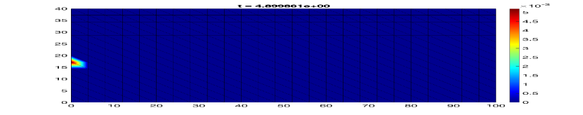
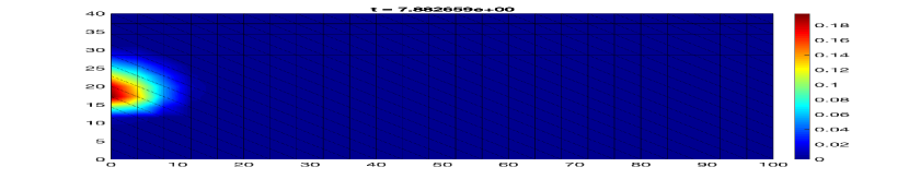
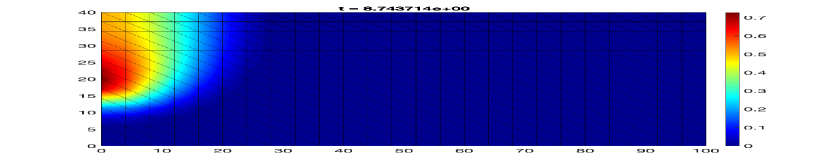
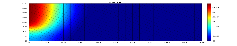
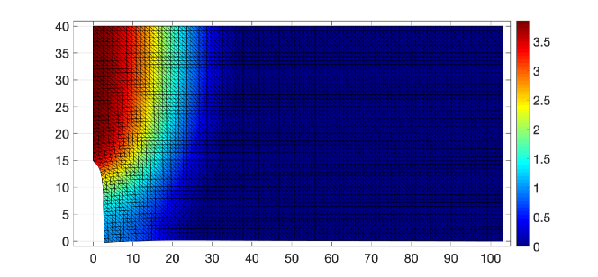
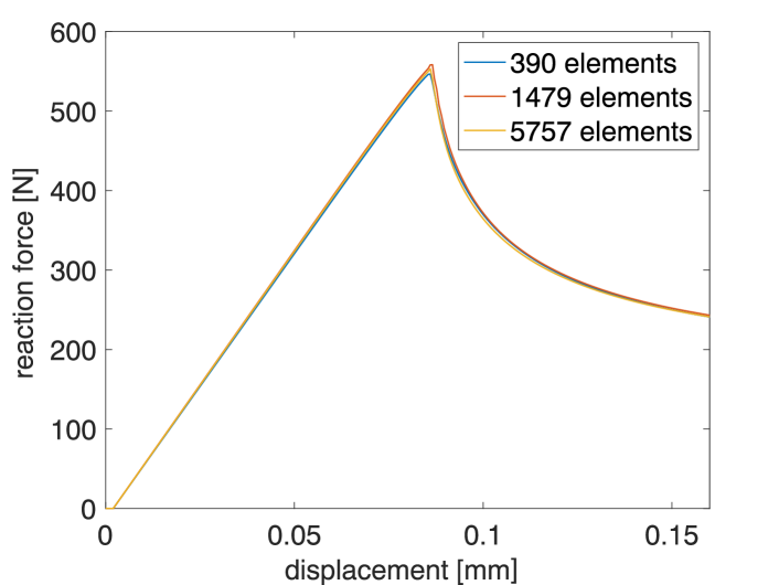
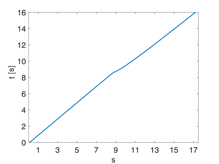
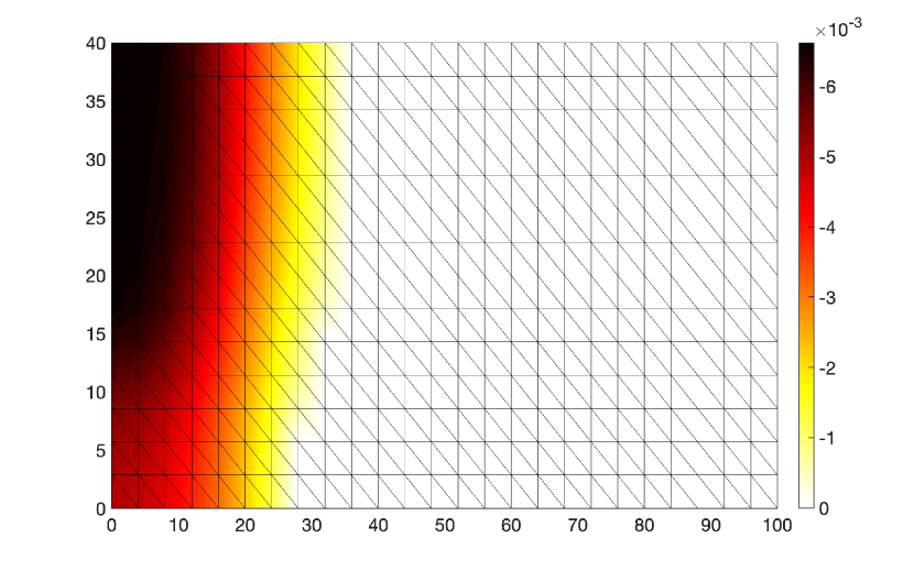
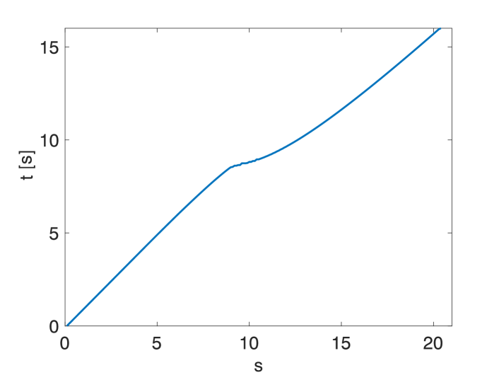
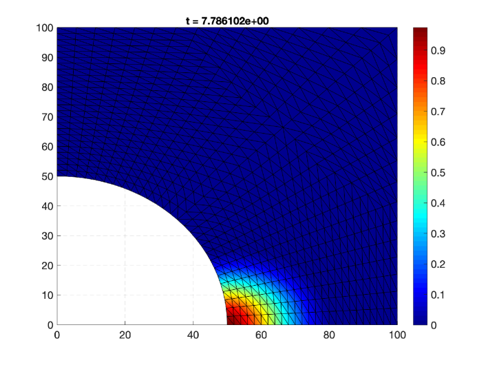
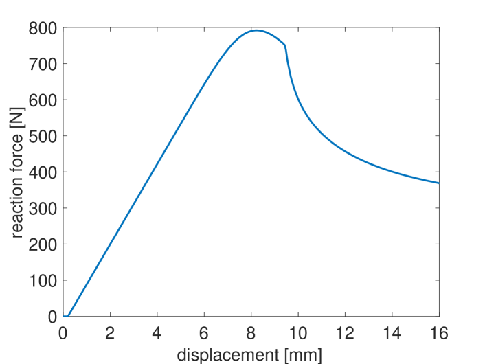
Furthermore, we use the parameters given in the table of Figure 4.1 (right). We initiate the evolution with and choose for the time step size. The state of damage at several points during the time interval are shown in Figure 4.2. Obviously, damage occurs at first at the tip of the crack and evolves along the symmetry axis afterwards. As expected, it also concentrates on regions with large stresses. However, the sharpness of interfaces between damaged and undamaged areas highly depends on the choice of the functional , see BMT (18). In our case, this interface is rather diffuse and cannot be sharpened by a refinement of the mesh, see Figure 4.3. Clearly, one may reduce the factor included in the operator . However, this leads to instabilities in the semismooth Newton method and globalization strategies might be necessary, which is subject of future research. Nevertheless, the results are stable with respect to mesh refinement, which can be observed in Figure 4.4 that shows the force-displacement-diagram for three different mesh sizes. The reaction force is calculated by integrating the stress in normal direction along the boundary . In comparison with the results from DH (08), there is a high degree of conformity, except for the larger values of the reaction force here after reaching its maximum at approximately of displacement, cf. also with Example II. With regard to the time function that is depicted in Figure 4.5 we see that the spreading of the damage area starting at is slightly faster than the rest of the evolution but does not cause a jump.
Let us finally compare the results obtained with an alternative approach. Instead of incorporating the constraint which corresponds to an -ball of size it is convenient to take . Indeed, as we have already imposed lower bounds for , namely , it seems appropriate from a numerical point of view to also include as a constraint since this leads to pointwise box constraints that are particularly well suited to semismooth Newton-methods, see e.g. HIK (02). Unfortunately, this choice is not covered by our convergence analysis for the local stationarity scheme ( (LISS).). Nevertheless, we provide the numerical results that can be obtained by using this version. Thus, while we change (4.15) to
| (4.16) |
we keep all parameters unaltered. Clearly, the Newton-matrix also changes in the obvious way. The difference between both solutions using (LISS). is shown in Figure 4.6. The time-function for the solution using box-constraints is given in Figure 4.7. It is easy to see that both solutions, using - and -constraints, are very similar. Indeed, the and distance at the end time calculates to . Since the incorporation of box constraints is natural in this context and its implementation is also easier to realize it provides an interesting topic for further research.
A possible approach for this is to consider the -Laplacian with for the regularization instead of as proposed in KRZ (15). In this case, we have which may open up the opportunity to use the -norm as constraint in (3.1).
Example II: Brick with a circular hole
As proof-of-concept we consider the situation depicted in Figure 4.8. Again, due to its symmetry the computation is performed using only one quarter of the whole system. This also implies certain symmetry conditions for the boundary of the domain . For the situation at hand, we impose
Moreover, the workpiece is pulled apart at two opposite sides, which we realize by the Dirichlet conditions
The parameters used are given in the table of Figure 4.8 (right). Finally, we initiate the evolution with and choose for the time step size. The numerical solution of the damage variable for an intermediate time point is shown in Figure 4.9 and the corresponding force-displacement-diagram is depicted in Figure 4.10. We observe a strong similarity with the results in DH (08). However, the reaction force in the end phase of the evolution is significantly higher in our case. This may be a result of the additional regularization by the introduction of a "local field" in DH (08). Certainly, this requires further investigation.
| parameters | |
|---|---|
| [MPa] | 0.1 |
| [GPa] (Young’s modulus) | 18.0 |
| (Poisson’s ratio) | 0.2 |
| [MPa] | 1.0 |
| [] | 100.0 |
| [] | 50.0 |
5 Conclusions
We presented a numerical scheme for the approximation of parametrized solutions for rate-independent systems including a fairly general setting for the energy and dissipation functionals. The scheme itself is based on the local minimization scheme introduced in EM (06), but relies on stationary points rather than local minima, making it very accessible for numerical optimization algorithms (limit points are, in general, stationary). Moreover, by adapting the convergence analysis of the recent contributions in Kne (19); MS19a and using arguments from KRZ (13), we proved that the scheme provides parametrized solutions of the original rate-independent system under Mosco-convergence of approximations for the dissipation . While this is at first glance a result that verifies the consistency of the local incremental stationarity scheme, we, moreover, gain an existence result for parametrized solutions in the case of a nonconvex energy and unbounded dissipation. We then focused on the realization of our scheme for a model of the evolution of damage within a workpiece. We employed a finite element discretization in space and used a semi-smooth Newton method for solving the discrete stationary system arising in each step of the scheme. The resulting algorithm behaves efficient and robust in our numerical tests. Afterall there are several topics for future research. This concerns for example the usage of an -norm in the indicator functional in (alg1) which leads to an easy to implement algorithm for the damage model considered in this paper. In the same context, it might be interesting to relax the assumptions for the energy in order to incorporate functionals that allow for a sharper resolution of the interface between damaged and undamaged regions. Moreover, considering dissipation functionals which are also depending on the state , i.e., should be noted here. As there are only few results in this direction for rate-independent systems this does not only concern parametrized solutions.
Acknowledgements.
I would like to thank Christian Meyer (TU Dortmund) for various discussions on the topic.Appendix A Auxiliary results from convex analysis
In this section, we collect some useful properties of and , respectively. Since most of the results are quite standard, we keep the arguments brief.
Lemma A.1.
Let be a normed vector space and a convex and positive 1-homogeneous functional. Then it holds
| (A.1a) | |||
| (A.1b) | |||
| (A.1c) | |||
| (A.1d) | |||
where denotes the indicator functional of .
Lemma A.2.
For every , there holds
| (A.3) |
where . Particularly, if there exists no such that . Moreover, if then there exists such that .
Proof.
We use the inf-convolution formula (see (Att, 84, Prop. 3.4)), which is applicable, since both functions are proper, convex and closed and we have . This gives
| (A.4) |
For , direct calculation leads to
| (A.5) |
Moreover, Lemma A.1 gives . Inserting this together with (A.5) in (A.4) finally yields
which is (A.3). Now, let and take such that . Obviously, this implies that is uniformly bounded in . Hence, we can extract a weakly convergent subsequence (w.l.o.g. denoted by the same symbol) such that in for some . Therefore, by the embedding , we have in which implies that . To proceed, we note that is again convex and closed and thus weakly closed in . Since for all we also have . Finally, the weak lower semicontinuity of the norm gives
which finishes the proof. ∎
In view of (alg1) we note that for any which can be easily obtained by considering the projection operator and applying the chain-rule for subdifferentials to . As in Remark 2.3 we nevertheless simply write . Moreover, we have the following characterization.
Lemma A.3.
Let be a reflexive Banach space and be arbitrary. Then, is an element of , iff
| (A.6) |
If is even a Hilbert space, then iff there exists a multiplier such that and
| (A.7) |
Proof.
According to a classical result of convex analysis in combination with (A.5), it holds
| (A.8) |
Hence, (A.6) follows easily from . Now, assume that is a Hilbert space. Then, the equality in (A.8) can only hold if for some . Inserting this into (A.8), we conclude that and so, if , then which gives (A.7). ∎
Appendix B Numerical aspects for the discrete energy functional
In this section we formally derive the necessary derivatives of used for the implementation of the local stationarity scheme in case of the damage model. We start with for which we note that by from (4.12), one obtains
| (B.1) |
Hence, with a little abuse of notation (particularly identifying and ) we have
The fact that moreover implies that
Therefore, for arbitrary , we can characterize as the solution of
| (B.2) |
Consequently, exploiting (B.1) it holds
with solving (B.2). Again, with a little abuse of notation we thus have
| (B.3) |
Now, let us turn to the semismooth Newton-method that is used in order to solve the stationary system in (4.15). In general, if we denote the left hand side of (4.15) by , equation (4.15) becomes and we need to solve the following semi-smooth Newton equation
with the iterate and a Newton-derivative . However, the matrix contains second order information of which, by (B.3) necessitates the determination of . In order to keep track of this, we blow up the whole system so that in every semismooth Newton-step we actually solve
with
| (B.4) |
Note that to shorten the notation we let . Moreover, we have
Eventually, we update , and . With this choice, all matrices appearing in our numerical test have shown to be invertible and the semi-smooth Newton method performed well with respect to both, robustness and efficiency. In particular, no globalization efforts are needed to ensure convergence of the method and, moreover, no line search was necessary in order to guarantee condition (alg2) in (LISS).. A rigorous convergence analysis of the method however would go beyond the scope of this paper and is subject to future research.
References
- (1)
- AB (19) Almi, S. ; Belz, S.: Consistent finite-dimensional approximation of phase-field models of fracture. In: Annali di Matematica Pura ed Applicata (1923-) 198 (2019), Nr. 4, S. 1191–1225
- ACFK (02) Alberty, J. ; Carstensen, C. ; Funken, S. A. ; Klose, R.: Matlab implementation of the finite element method in elasticity. In: Computing 69 (2002), Nr. 3, S. 239–263
- Alt (16) Alt, H.W.: Linear Functional Analysis: An Application-Oriented Introduction. Springer, 2016
- AMS (08) Auricchio, F. ; Mielke, A. ; Stefanelli, U.: A rate-independent model for the isothermal quasi-static evolution of shape-memory materials. In: Mathematical Models and Methods in Applied Sciences 18 (2008), Nr. 01, S. 125–164
- Att (84) Attouch, H.: Variational Convergence for Functions and Operators. Pitman Advanced Publishing Program, 1984
- BMT (18) Bartels, S. ; Milicevic, M. ; Thomas, M.: Numerical approach to a model for quasistatic damage with spatial BV-regularization. In: Trends in Applications of Mathematics to Mechanics (2018), S. 179–203
- Bon (96) Bonfanti, G.: A vanishing viscosity approach to a two degree-of-freedom contact problem in linear elasticity with friction. In: Annali dell’Universita di Ferrara 42 (1996), Nr. 1, S. 127–154
- DH (08) Dimitrijevic, B.J. ; Hackl, K.: A method for gradient enhancement of continuum damage models. In: Technische Mechanik-European Journal of Engineering Mechanics 28 (2008), Nr. 1, S. 43–52
- EM (06) Efendiev, M. A. ; Mielke, A.: On the rate-independent limit of systems with dry friction and small viscosity. In: J. Convex Analysis 13 (2006), Nr. 1, S. 151–167
- FM (06) Francfort, G. ; Mielke, A.: Existence results for a class of rate-independent material models with nonconvex elastic energies. In: J. Reine Angew. Math. (2006), Nr. 595, S. 55–91
- Gia (05) Giacomini, A.: Ambrosio-Tortorelli approximation of quasi-static evolution of brittle fractures. In: Calculus of Variations and Partial Differential Equations 22 (2005), Nr. 2, S. 129–172
- Grö (89) Gröger, K.: A -estimate for solutions to mixed boundary value problems for second order elliptic differential equations. In: Mathematische Annalen 283 (1989), Nr. 4, S. 679–687
- HIK (02) Hintermüller, M. ; Ito, K. ; Kunisch, K.: The primal-dual active set strategy as a semismooth Newton method. In: SIAM J. Optim. 13 (2002), Nr. 3, 865–888 (2003). http://dx.doi.org/10.1137/S1052623401383558. – DOI 10.1137/S1052623401383558
- HMW (11) Herzog, R. ; Meyer, C. ; Wachsmuth, G.: Integrability of displacement and stresses in linear and nonlinear elasticity with mixed boundary conditions. In: J. Math. Anal. Appl. 382 (2011), Nr. 2, S. 802–813
- Kne (19) Knees, D.: Convergence analysis of time-discretisation schemes for rate-independent systems. In: ESAIM: Control Optim. Calc. Var. 25 (2019), S. 65
- KRZ (13) Knees, D. ; Rossi, R. ; Zanini, C.: A vanishing viscosity approach to a rate-independent damage model. In: Math. Models Methods Appl. Sci. 23 (2013), Nr. 04, S. 565–616
- KRZ (15) Knees, Dorothee ; Rossi, Riccarda ; Zanini, Chiara: A quasilinear differential inclusion for viscous and rate-independent damage systems in non-smooth domains. In: Nonlinear Analysis: Real World Applications 24 (2015), S. 126–162
- Mai (04) Mainik, A.: A rate-independent model for phase transformations in shape-memory alloys, Universität Stuttgart, Diss., 2004. http://dx.doi.org/10.18419/opus-4749. – DOI 10.18419/opus–4749
- MM (09) Mainik, A. ; Mielke, A.: Global existence for rate-independent gradient plasticity at finite strain. In: J. Nonlin. Sci. 19 (2009), Nr. 3, S. 221–248
- MMMG (94) Martins, JA C. ; Monteiro Marques, MD P. ; Gastaldi, Fabio: On an example of non-existence of solution to a quasistatic frictional contact problem. In: European Journal of Mechanics - A./Solids 13 (1994), Nr. 1, S. 113–133
- MR (15) Mielke, A. ; Roubíc̆ek, T.: Rate-Independent Systems: Theory and Application. New York : Springer, 2015
- MRS (09) Mielke, A. ; Rossi, R. ; Savaré, G.: Modeling solutions with jumps for rate-independent systems on metric spaces. In: Discrete & Continuous Dynamical Systems-A 25 (2009), Nr. 2, S. 585–615
- MRS (16) Mielke, A. ; Rossi, R. ; Savaré, G.: Balanced viscosity (BV) solutions to infinite-dimensional rate-independent systems. In: J. Eur. Math. Soc. (JEMS) 18 (2016), Nr. 9, S. 2107–2165
- MS (17) Matteo, N. ; Scala, R.: A quasi-static evolution generated by local energy minimizers for an elastic material with a cohesive interface. In: Nonlinear Anal.: Real World Appl. 38 (2017), S. 271–305
- (26) Meyer, C. ; Sievers, M.: Finite Element Discretization of Local Minimization Schemes for Rate-Independent Evolutions. In: Calcolo 56 (2019), Nr. 6. http://dx.doi.org/10.1007/s10092-018-0301-4. – DOI 10.1007/s10092–018–0301–4
- (27) Meyer, C. ; Susu, L.M.: Analysis of a Viscous Two-Field Gradient Damage Model II: Penalization Limit. In: Zeitschrift für Analysis und ihre Anwendungen 38 (2019), Nr. 4, S. 439–474
- MSGMM (95) Martins, J.A.C. ; Simões, F.M.F. ; Gastaldi, F. ; Monteiro Marques, M.D.P.: Dissipative graph solutions for a 2 degree-of-freedom quasistatic frictional contact problem. In: International journal of engineering science 33 (1995), Nr. 13, S. 1959–1986
- MZ (14) Mielke, A. ; Zelik, S.: On the vanishing-viscosity limit in parabolic systems with rate-independent dissipation terms. In: Ann. Sc. Norm. Super. Pisa, Cl. Sci. 13 (2014), Nr. 1, S. 67–135
- Neg (14) Negri, M.: Quasi-static rate-independent evolutions: characterization, existence, approximation and application to fracture mechanics. In: ESAIM Control Optim. Calc. Var. 20 (2014), Nr. 4, S. 983–1008. http://dx.doi.org/10.1051/cocv/2014004. – DOI 10.1051/cocv/2014004
- Sie (20) Sievers, M.: A Numerical Scheme for Rate-Independent Systems - Analysis and Realization, Technische Universität Dortmund, Diss., 2020. http://dx.doi.org/http://dx.doi.org/10.17877/DE290R-21874. – DOI http://dx.doi.org/10.17877/DE290R–21874
- Ste (08) Stefanelli, Ulisse: The Brezis–Ekeland principle for doubly nonlinear equations. In: SIAM J. Control Optim. 47 (2008), Nr. 3, S. 1615–1642