Interpretable Semantic Photo Geolocation

Abstract

Planet-scale photo geolocalization is the complex task of estimating the location depicted in an image solely based on its visual content. Due to the success of convolutional neural networks (CNNs), current approaches achieve super-human performance. However, previous work has exclusively focused on optimizing geolocalization accuracy. Due to the black-box property of deep learning systems, their predictions are difficult to validate for humans. State-of-the-art methods treat the task as a classification problem, where the choice of the classes, that is the partitioning of the world map, is crucial for the performance. In this paper, we present two contributions to improve the interpretability of a geolocalization model: (1) We propose a novel semantic partitioning method which intuitively leads to an improved understanding of the predictions, while achieving state-of-the-art results for geolocational accuracy on benchmark test sets; (2) We introduce a metric to assess the importance of semantic visual concepts for a certain prediction to provide additional interpretable information, which allows for a large-scale analysis of already trained models. Source code and dataset are publicly available.

1 Introduction

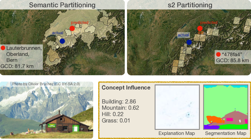
Figure 1: Example output of a geolocalization model with our proposed semantic partitioning for more explainable geolocation estimation (left) compared to an existing partitioning approach (right). Additionally, we measure the influence of visible concepts on the prediction of a model given an explanation and segmentation map.

Image geolocalization is the challenging task of predicting the location of a photo in form of GPS coordinates based only on its visual content. Almost all state-of-the-art approaches for planet-scale image geolocalization [45, 21, 33] define the task as a classification problem, where the earth is divided into geographical cells (called partitioning), and train Convolutional Neural Networks (CNNs) with a huge amount of labeled data in an end-to-end fashion. This strategy and the large amount of parameters in the networks turn them into a kind of black-box-systems, whose reasoning and predictions are not comprehensible –  making it necessary to develop methods to understand their decisions [5, 7]. This is particularly a requirement for geolocalization systems for two reasons. First, humans are far worse at estimating locations than current deep learning approaches [45]; second, research has focused exclusively on maximizing localization accuracy, but lacks proposals for interpretable and explainable models.

While many approaches (e.g., [2, 30, 22, 42, 31]) restrict the problem of photo geolocalization to a part of the earth (e.g., landmarks or mountains), predicting coordinates at planet-scale without any restrictions is more complex. Landmarks (usually tourist attractions) can partly be verified by humans, whereas many photos give little indication of the actual place or region. As a result, the question arises which features have been learned and which image features are relevant for a given prediction. Furthermore, the quadratic boundaries of the s2 partitioning [45] are arbitrary (see Figure 1) and the cells of CPlaNet [33] are initialized randomly which is counter-intuitive with regard to comprehensibility. Following these considerations, a CNN-based approach for geolocation estimation should therefore also be assessed with regard to the interpretability of its results.

In this paper, we address this issue and introduce a novel semantic partitioning (SemP)method where the cells are not rectangular or arbitrarily shaped as in previous approaches [45, 33, 21]. Instead, the partitioning considers real and interpretable locations derived from territorial (e.g., streets, cities, or countries), natural (e.g., rivers, mountains), or man-made boundaries (e.g., roads, railways, or buildings) extracted from Open Street Map (OSM) [24] data (Figure 1). This partitioning better reflects location entities and we argue that photos taken within these boundaries also more likely share similar geographic attributes. As a result, training and output of a model are more comprehensible to humans by default, while at the same time, state-of-the-art results on common test sets are achieved. In addition, we suggest a concept influence metric to investigate the post-hoc interpretability by measuring the influence of semantic visual concepts on individual predictions (example in Figure 1). Experimental results show that the novel semantic partitioning method achieves (at least) state-of-the-art performance, while the concept influence score provides insights which visual concepts contribute to correct and incorrect (or misleading) predictions.

The rest of the paper is organized as follows. Related work for photo geolocation estimation is reviewed in Section 2. The novel semantic partitioning method and concept influence score are described in Section 3, while experimental results are reported in Section 4, both for accuracy and interpretability of the results. Section 5 summarizes the paper and outlines areas of future work.

2 Related Work

Whereas only few approaches [45, 43, 21, 33, 13] are applicable at planet-scale without limitations, the majority simplifies the task of geolocalization, for example, by predicting landmarks and cities [2, 46, 30, 22], natural areas [3, 18, 32, 42, 31], or geo-related attributes [17].

Previous work uses either image retrieval approaches or models the task as a classification problem. The task of geolocation estimation at planet-scale has an overlap with methods from instance-level image retrieval [22, 2, 6, 27, 41] where benchmark datasets consist of popular places, landmarks, and tourist attractions [25, 26, 14] which can be verified by humans. Common to all is the usage of triplet ranking or contrastive embeddings to learn discriminative image representations, whereas Liu et al. [19] introduce an alternative loss function. These representations are used to retrieve the most similar images in a reference database in order to determine the geolocation as proposed by Im2GPS [8, 9]. Weyand et al. [45] introduce the classification approach PlaNet, where a GPS coordinate is mapped to a discrete class label using a quad-tree approach that divides the surface of the earth into distinct regions using the s2 geometry library [29]. This s2 partitioning is used at multiple spatial scales to exploit hierarchical knowledge [43, 21]. A pre-classification step assigns a photo to one of three scene types (natural, urban, indoor) and leads to improvements [21]. Seo et al. [33] propose a combinatorial partitioning where the overlaps of multiple coarse-grained partitionings create one fine-grained partitioning. Izbicki et al. [13] introduce the Mixture of von-Mises Fisher (MvMF) loss function for the classification layer that exploits the earth’s spherical geometry and refines the geographical cell shapes in the partitioning. Kordopatis-Zilos et al. [15] combine classification [13, 21] and retrieval techniques to leverage the advantages of each approach, i.e., learning global knowledge from classification and exploit local features via retrieval (landmark matching).

3 Interpretable Semantic Photo Geolocation

As the discussion of related work reveals, all approaches (classification and retrieval) rely on features from CNNs that are learned with the use of a partitioning. Their predictions are difficult to interpret and the construction of the partitioning is crucial for the system performance [43, 33]. The following two subsections address two issues with regard to interpretability. First, a novel partitioning method is proposed that relies on data that are derived from a geographic database where metadata about many regions and places such as their size or exact boundaries is provided. Second, a method is presented to automatically assess image features that are relevant for a model’s decision based on semantic visual concepts like waterfall or person. Their workflows and connections are outlined in Figure 2.

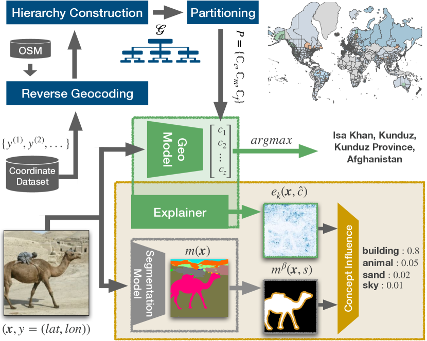
Figure 2: Overview of the bipartite system: Top (blue): Workflow to create a semantic partitioning (SemP), bottom (orange): Components to measure the concept influence for individual samples.

3.1 Semantic Partitioning

State-of-the-art methods for photo geolocalization rely on classification approaches [33, 21], where the design of the classification layer is crucial for the model’s output with respect to prediction accuracy, but also regarding the information that is provided to users. The main idea is to divide the earth surface into a discrete set of classes $\mathbb{C}$ based on the dataset distribution to then train a classification network [45]. We follow the same idea, but after all our cells cover territorial borders (e.g., countries, cities), natural geological boundaries (e.g., rivers, mountains) or man-made barriers (e.g., roads or railways that separate districts). In addition to an improved understanding of the created cells, the assumption is that a CNN learns better image representations, since the resulting geographic cells might better represent locations and are thus more distinguishable. The following steps describe formally how that semantic partitioning (SemP)is constructed.

3.1.1 Reverse Geocoding & Hierachy Construction

Following the idea of classification, a mapping is needed from the continuous GPS coordinate space to a discrete set of existing locations which is called reverse geocoding. Frameworks for reverse geocoding generate an address vector, e.g., (Long Beach, Los Angeles County, California, USA) with a coordinate as input. We choose Nominatim [23] since it is open source software and relies on OSM. Formally, a reverse geocoder maps each coordinate $y^{(i)}=(\text{latitude},\text{longitude})$ in a dataset $\mathbb{D}=\{y^{(1)},y^{(2)},\ldots\}$ to an address vector $\boldsymbol{l}^{(i)}=(l_{1},\ldots,l_{u})$ of arbitrary length $u$ and is ordered from fine to coarse. This mapping is denoted as $\mathbb{D}^{l}=\{\boldsymbol{l}^{(1)},\boldsymbol{l}^{(2)},\ldots\}$.

Hierarchy Construction: Since hierarchical knowledge is valuable with respect to performance [45, 21] and all necessary information is already provided by the reverse geocoder, we construct a hierarchy similar to the s2 library [45] but with semantically meaningful nodes and edges. In order to create a partitioning from the obtained addresses $\mathbb{D}^{l}$, it is required to build a hierarchy where each discrete location $l$ (e.g., Long Beach) can be assigned to its next coarser distinct location (e.g., Los Angeles County). A directed (multi-) graph $\mathcal{G}=(V,E)$ can be constructed using all edges that occur in the mapping $\mathbb{D}^{l}$. The total number of nodes corresponds to the number of locations; an edge exists between two adjacent nodes encoded in the mapping $\mathbb{D}^{l}$, i.e., $(l_{i},l_{i+1})\forall i\in[1,\ldots,u-1]$ for every $\boldsymbol{l}=(l_{1},\ldots,l_{u})\in\mathbb{D}^{l}$. Nodes without outgoing edges (roots) usually correspond to countries. Ideally, $\mathcal{G}$ consists only of trees, where exactly one parent node is assigned to each node with the exception of the root nodes. Otherwise, $\mathcal{G}$ must be transformed into a hierarchy. For each location only the most frequent outgoing edge is kept. Reasons for multiple parents are possible incorrect assignments for some instances or missing assignments that cause shortcuts. Therefore, the mapping $\mathbb{D}^{l}$ is subsequently replaced with the locations from the shortest path of the finest location $l_{1}$ in $(l_{1},...,l_{u})=\boldsymbol{l}\quad\forall\boldsymbol{l}\in\mathbb{D}^{l}$ to its root node in the hierarchy $\mathcal{G}$ and is referred to as $\mathbb{D}^{l^{*}}$.

3.1.2 Partitioning Construction & Cell Assignment

In order to create the SemP, the set of coordinates $\mathbb{D}$ is first transformed to a (hierarchical) multi-label dataset as described in Section 3.1.1. A valid partitioning would be to consider only the finest location $l^{(i)}_{1}$ for each $\boldsymbol{l}^{(i)}$. In practice, a huge number of classes is not manageable and previous work (e.g., [45]) controls the granularity of a partitioning. This choice of granularity entails a trade-off problem. While fewer but larger (in terms of geographic area) cells decrease the geospatial resolution of the model outputs, more but smaller cells are more challenging to distinguish. They also make the model susceptible to overfitting due to the lower number of available training images per cell [33]. Moreover, geographic information at different spatial resolutions are important to identify locations of varying granularity (e.g., buildings, cities, or countries). To construct a partitioning $\mathbb{C}$ at a certain spatial level, we first delete all locations from the derived hierarchy $\mathcal{G}$ with less than $\tau_{\text{min}}$ images. As a result, we derive a mapping $\mathbb{D}^{l^{*}}$ with the remaining locations in the graph. The finest locations in $\mathbb{D}^{l^{*}}$ form a partitioning, i.e., all $l_{1}$ from all $\boldsymbol{l}\in\mathbb{D}^{l^{*}}$. To assign a dataset $\mathbb{D}_{\text{new}}$ to classes from a created partitioning $\mathbb{C}$, two steps are necessary. First, the same reverse geocoder has to create an initial assignment $\mathbb{D}^{l^{*}}_{\text{new}}$ and these discrete locations are filtered by the available locations (now classes) from the partitioning $\mathbb{C}$. Given the $i$-th sample $\boldsymbol{l}^{(i)}\in\mathbb{D}^{l^{*}}_{\text{new}}$, the location $l^{(i)}_{1}$ from $\boldsymbol{l}^{(i)}$ corresponds to the finest available one according to the partitioning $\mathbb{C}$.

3.1.3 Learning & Inference

With the classes $\mathbb{C}$ obtained from the presented partitioning method, a CNN can be trained directly on the classification task using the cross-entropy loss ($\mathcal{L_{\text{CE}}}$) where the number of classes corresponds to the number of cells of the partitioning. Initially, only a dataset of image-coordinate pairs is necessary where the coordinates are transformed to classes according to Section 3.1.2. Multiple partitionings can be combined to force the model to learn some kind of hierarchical knowledge. Given a tuple of partitionings $\mathcal{P}=(\mathbb{C}_{1},...,\mathbb{C}_{n})$ which differ only in $\tau_{\text{min}}$ (i.e., controls the number of classes) and are ordered from fine to coarse, each cell in $\mathbb{C}_{i}$ can be assigned to its corresponding cell in $\mathbb{C}_{i+1}$ by exploiting the hierarchy $\mathcal{G}$. One fully-connected layer per partitioning $\mathbb{C}_{i}$ is added on top of an appropriate CNN architecture. During training, the multi-partitioning classification loss is defined as the sum of all individual losses per partitioning $\mathcal{L}_{\text{CE}}^{\text{multi}}=\sum_{i=1}^{|\mathcal{P}|}\mathcal{L}_{\text{CE}}^{i}$. During inference, the class at the finest partitioning with the highest probability after applying the softmax function corresponds to the predicted cell $\hat{c}$. We use the average GPS coordinate of the assigned samples from $\mathbb{D}$ during the partitioning process from the respective class as geolocation prediction.

3.2 Measuring the Input Feature Importance

In the task of photo geolocalization, we do not know which image regions are crucial for the model’s prediction and cannot validate the decisions. While methods for the visualization of feature attributions have been researched in recent years, the main focus was on object recognition where the highlighted areas are comprehensible at least to humans [1]. Inspired by these approaches, we propose a method to measure the influence of specific objects (e.g., vehicle or person) and semantic image regions (e.g., sky or ground) regarding the model’s prediction. The goal is not to identify a concrete concept that is responsible for the prediction – which would be counter intuitive, since a decision should not be reduced to image regions exclusively. Rather it can be helpful to estimate the overall impact of a given semantic concept, to identify misleading concepts, or to provide explanatory information in form of a more comprehensible (text and quantitative values) and summarized (reduced to relevant concepts) explanation map to users. Attribution maps also provide an importance value per pixel, but also a lot of noise [35] and allow the observer freedom in the interpretation.

Required Components:

Formally, an input image $\boldsymbol{x}\in\mathbb{R}^{w\times h\times d}$ and a CNN $\Psi$ are required. Only two components are needed to calculate the influence of concepts on the prediction. An explanation map $e$ assigns an importance score to each input pixel of $\boldsymbol{x}$ for a certain prediction [38, 34, 36], e.g., a target class $\hat{c}$ in case of a classification model. The maximum over the (color) channel dimension $d$ is taken as only image regions are of interest, hence we define $e:\mathbb{R}^{w\times h\times d}\mapsto\mathbb{R}^{w\times h}$. Please note, that usually only the gradients of the model $\Psi$ have to be accessible for the calculation. A segmentation map $m$ divides image areas into semantic groups (e.g., a region, object, or texture). The segmentation mask for one concept $s\in\mathbb{S}$ is the indicator function where the presence of $s$ on a pixel is indicated by $m:\mathbb{R}^{w\times h\times d}\mapsto\{0,1\}^{w\times h}$ and denoted as $m(\boldsymbol{x},s)$.

Assuming that the area of the segmentation boundaries, i.e., the border between two concepts is of interest for the geo model resulting in activations in the explanation map, the active area of the binary mask $m(\boldsymbol{x},s)$ for concept $s$ can be enlarged $\beta$ pixels around its shape boundary using a morphological dilation, and is denoted as $m^{\beta}(\boldsymbol{x},s)$ as seen in Figure 2 (orange colorized area around the camel’s surface).

Concept Influence:

The aim is to measure the influence of a specific concept $s$ using the explanation map $e(\boldsymbol{x},\hat{c})$ and the segmentation map $m(\boldsymbol{x},s)$ for a specific concept $s$. As stated by Ghorbani et al. [4], in many settings only the most important features are of explanatory interest. They compute the pixel-wise intersection of the $k$ most important features from $e(\boldsymbol{x},\hat{c})$ to measure the difference between two explanation maps (top-$k$ intersection). However, this is done for a slightly different purpose, that is generating and evaluating manipulated explanation maps. Inspired by this, we adapt this measure to define the influence of a concept $s$ visible in image $\boldsymbol{x}$ with respect to a geoprediction $\hat{c}$ of the model. We define the pixel-wise intersection $tki$ between the binary segmentation mask $m(\boldsymbol{x},s)$ and the binary mask of the top-$k$ features $e_{k}(\boldsymbol{x},\hat{c})$ as

$$tki=\frac{1}{k}\sum_{i=1}^{w}\sum_{j=1}^{h}m(\boldsymbol{x},s)_{i,j}\wedge e_{k}(\boldsymbol{x},\hat{c})_{i,j}$$ (1)

where $m(\boldsymbol{x},s)$ and $e_{k}(\boldsymbol{x},\hat{c})$ are both in $\{0,1\}^{w\times h}$ and $\wedge$ is the pixel-wise boolean and operation. For instance, if all top-$k$ pixels are within the shape of the concept $s$ then $tki=1$. In our experiments, we set the parameter $k$ to 1,000 as proposed by Ghorbani et al. [4]. As large objects or areas are preferred, a normalization step is crucial for application. The defined top-$k$ intersection (tki) is hence normalized by the relative size of the concept which is defined as:

$$\overline{s}:=\frac{1}{wh}\sum_{i=1}^{w}\sum_{j=1}^{h}\big{(}m(\boldsymbol{x},s)\big{)}_{i,j}$$ (2)

The resulting score is the definition of the concept influence (ci) metric $ci\big{(}m(\boldsymbol{x},s),e_{k}(\boldsymbol{x},\hat{c})\big{)}=tki/\overline{s}$. A ci score of less than or equal to one means that the top-$k$ pixels of the explanation map are more likely to be in other regions of the image, i.e., class $s$ has little or no influence on the final prediction. The ci score indicates whether a concept $s$ contains relatively large number of activations of the explainer $e$. When fixing the minimum required relative concept size to $0<\overline{s}_{\text{min}}<1$, ci $\in[0,\frac{1}{\overline{s}_{\text{min}}}]$ is well defined and only those concepts are considered for the calculation that cover at least this area. Additionally, we assume that small concepts that cover only a minimal area in the image to be irrelevant or noisy and set $\overline{s}_{\text{min}}=0.05$ in our experiments.

Finally, given a segmentation map $m$ and an explanation map $e$ for model $\Psi$, the introduced metric ci automatically measures the impact of semantic image regions for the prediction.

4 Experimental Results

In this section, the proposed partitioning method is evaluated with respect to geolocational accuracy and its capability of providing an improved interpretability (Section 4.1). Afterwards, the concept influence metric introduced in Section 3.2 is evaluated (Section 4.2).

4.1 Semantic Partitioning

We demonstrate the capability of our approach through a comparison with several state-of-the-art models, including a model that also exploits the hierarchical knowledge from multiple partitionings [21], on three benchmark datasets.

4.1.1 Experimental Setup

Datasets & Evaluation Metric: We utilize the MediaEval Placing Task 2016 (MP-16) [16] dataset which is a subset from the Yahoo Flickr Creative Commons 100 Million (YFCC100M) [40] both for partitioning construction and training. Its only restriction is that an image contains a GPS coordinate, thus it contains images of landmarks, landscape images, but also images with little to no geographical cues. Like Vo et al. [43], images are excluded from training if there are photos taken by the same authors in the Im2GPS3k test set and duplicates are removed, resulting in a dataset size of 4,723,695 image-coordinate pairs. For validation, a randomly sampled subset of 25,600 images from YFCC100M without overlap to the training images is created and denoted as YFCC-Val26k. For testing, we focus on three popular benchmark datasets: YFCC4K [43] comes from the same image domain as the training dataset but is designed for general computer vision tasks making the test set more challenging. In contrast, the Im2GPS [8] and Im2GPS3k [43] datasets contain some landmarks, but the majority of images is recognizable only in a generic sense like landscapes.

For evaluation, the geolocational accuracy at multiple error levels, i.e., the tolerable error in terms of distance from the predicted $l_{\text{pred}}$ to the ground-truth location $l_{\text{gt}}$ is calculated [45, 43]. Formally, the geolocational accuracy $a_{r}$ at scale $r$ (in km) is defined as follows for a set of $N$ samples:

$$a_{r}\equiv\frac{1}{N}\sum_{i=1}^{N}u\left(d(l_{\text{gt}}^{(i)},l_{\text{pred}}^{(i)})<r\right),$$ (3)

where the distance function is the Great Circle Distance (GCD)and $u(\cdot)$ is the indicator function whether the distance is smaller than the tolerated radius $r$.

Partitioning Parameters: First, the coordinates from the MP-16 are transformed to a multi-label dataset containing 2,191,616 unique locations. To initially reduce the number, we delete all locations with less then 50 images. resulting in manageable 46,240 unique locations. Due to the proven importance of a multi-partitioning [43, 33, 21], we directly evaluate this setting. For a fair comparison, we construct a multi-partitioning that consists of three individual partitionings (coarse, middle, fine) with a similar total number of unique classes compared to Müller-Budack et al. [21] and follow their notation. To construct a multi-partitioning, several thresholds $\tau_{\text{min}}$ can be applied to get a similar number of classes, as shown in Table 1. For this reason, we select the model that performs best on the validation set for the comparison and evaluation on the test sets. Furthermore, we investigate three additional settings: (1) To keep the parameters fixed, but applying one filter, i.e., utilization of locations that are associated with geographic area stored as a (multi-)polygon according to OSM (denoted as $\lx@glossaries@gls@link{main}{ah}{\leavevmode\emph{SemP}}_{a}$); (2) testing the hierarchical prediction variant ($f$ vs. $f^{*}$); and (3) testing the scalability by doubling the number of classes.

Table 1: Experimental results on the validation set of YFCC-Val26k for several multi-partitonings where $|\mathbb{C}|$ is the total number of unique classes.

Configuration	$|\mathbb{C}|$	$a_{r}$ [%] @ km
		1	25	200	750	2500
$\text{\lx@glossaries@gls@link{main}{ah}{\leavevmode\emph{SemP}}}(\{100,125,150\},f^{*})$	14877	4.8	11.0	18.5	33.6	53.9
$\text{\lx@glossaries@gls@link{main}{ah}{\leavevmode\emph{SemP}}}(\{100,125,150\},f)$	14877	7.5	15.8	23.8	38.0	56.6
$\text{\lx@glossaries@gls@link{main}{ah}{\leavevmode\emph{SemP}}}_{a}(\{100,150,250\},f)$	12886	6.2	16.1	24.4	38.0	55.3
$\text{\lx@glossaries@gls@link{main}{ah}{\leavevmode\emph{SemP}}}(\{100,150,250\},f)$	15127	6.6	16.4	24.0	37.6	55.4
$\text{\lx@glossaries@gls@link{main}{ah}{\leavevmode\emph{SemP}}}(\{100,125,250\},f)$	15016	7.5	15.9	24.1	38.3	56.6
$\text{\lx@glossaries@gls@link{main}{ah}{\leavevmode\emph{SemP}}}_{a}(\{75,100,150\},f)$	16808	6.6	16.4	24.0	37.6	55.4
$\text{\lx@glossaries@gls@link{main}{ah}{\leavevmode\emph{SemP}}}(\{50,75,100\},f)$	34049	8.9	16.6	24.1	37.9	56.3
$s_{2}(M,f^{*})$	15606	6.8	16.4	24.6	38.4	56.8

Network Training & Inference: We choose the commonly applied ResNet-50 [10, 11] and EfficientNet-B4 [39] as network architectures with an input dimension of $224\times 224\times 3$ and $300\times 300\times 3$, respectively. As the ResNet-50 provides a good trade-off in terms of training time and performance, it is applied for the ablation study (testing several partitioning parameters). The classification layers are added on top of the global pooling layer. Instead of initializing the parameters of all models with ImageNet weights, the weights from a model trained for ten epochs on countries is taken to derive features related to the problem. The SGD method with an initial learning rate of $0.01$, a momentum of $0.9$, and weight decay of $10^{-4}$ is used to optimize for 15 epochs. The learning rate is exponentially decreased by a factor of 0.5, initially after every three epochs, and every epoch from epoch 12 on. Training is performed with a batch size of 200 and validation is done after 512,000 images. Details for pre-training and image augmentation methods during training are reported in the appendix. The model with the lowest loss $\mathcal{L}_{\text{CE}}^{\text{multi}}$ on the validation set is chosen. During inference, five crops are made and the mean prediction after applying softmax is taken.

4.1.2 Results on the Validation Set

The geolocational accuracies on the YFCC-Val26k validation set are reported in Table 1. Results demonstrate that the exact choice of partitioning hyperparameters is not essential. All configurations with similar number of classes perform similarly well. Surprisingly, the hierarchical prediction ($f^{*}$) [21] is, in contrast to the assumptions, worse than considering only the finest partitioning ($f$). One technical reason might be the fundamental different underlying structure of the hierarchy $\mathcal{G}$ in contrast to the quad-tree [45], resulting in a significantly lower depth and more variable number of child nodes. Humans may perceive locations hierarchically, but these coarse regions are not the ones with visually discriminative features.

4.1.3 Benchmark Results

From the models evaluated on the validation set, we select the one that has the best geolocational accuracy ($\text{\lx@glossaries@gls@link{main}{ah}{\leavevmode\emph{SemP}}}(\{100,125,250\},f)$), particularly for the error levels of 1 km, 750 km, and 2,500 km. Further, we assess the performance of one model considering only locations where geographic areas are available ($\text{\lx@glossaries@gls@link{main}{ah}{\leavevmode\emph{SemP}}}_{a}(\{100,150,250\},f$), and where the number of classes is doubled ($\text{\lx@glossaries@gls@link{main}{ah}{\leavevmode\emph{SemP}}}(\{50,75,100\},f)$). As stated in the experimental setup, we test these configurations with two different CNN backbones. Quantitative results are reported for three test sets in Table 2.

Table 2: Geolocational accuracy ($a_{r}$) of SemP compared to several geolocalization approaches on common benchmark datasets. ResNet-50 and EfficientNet-B4 are applied for fair comparisons to the state of the art. Retrieval extensions and ensembles typically improve the performance and are colored gray.

	$a_{r}$ [%] @ km
Approach	1	25	200	750	2500
Im2GPS3k [43] (2,997 images): geo-recognizable (generic)
[L]7011C [43]	4.0	14.8	21.4	32.6	52.4
[L]kNN, $\sigma=4$ [43]	7.2	19.4	26.9	38.9	55.9
PlaNet [45] (rep.) [33]	8.5	24.8	34.3	48.4	64.6
CPlaNet[1-5, PlaNet] [33]	10.2	26.5	34.6	48.6	64.6
MvMF${}_{\text{B4}}$ (rep. [15])	13.1	29.8	38.0	52.3	67.6
$ISN(M,f^{*},S_{3})$ [21]	10.5	28.0	36.6	49.7	66.0
$s2_{\text{B4}}(M,f^{*})$ (rep. [15]) + RRM	13.2	29.1	37.8	52.0	68.1
MvMF${}_{\text{B4}}$ (rep. [15]) + RRM	15.0	30.0	38.0	52.3	67.6
$s2_{\text{B4}}(M,f^{*})$ (rep.)	11.5	30.8	41.0	55.7	70.8
$\text{{\lx@glossaries@gls@link{main}{ah}{\leavevmode\emph{SemP}}}}_{\text{B4}}(\{100,125,250\},f)$	12.5	31.4	42.7	57.3	72.0
$\text{{\lx@glossaries@gls@link{main}{ah}{\leavevmode\emph{SemP}}}}_{\text{B4}}(\{50,75,100\},f)$	13.5	30.8	41.2	54.7	70.2
$s2(M,f^{*})$ [21]	9.7	27.0	35.6	49.2	66.0
$s2(M,f^{*})$ (rep.)	10.0	27.0	36.5	50.9	67.2
$\text{{\lx@glossaries@gls@link{main}{ah}{\leavevmode\emph{SemP}}}}(\{100,125,250\},f)$	11.1	27.1	36.7	50.4	66.1
$\text{{\lx@glossaries@gls@link{main}{ah}{\leavevmode\emph{SemP}}}}_{a}(\{100,150,250\},f)$	9.6	26.9	36.8	49.7	65.1
$\text{{\lx@glossaries@gls@link{main}{ah}{\leavevmode\emph{SemP}}}}(\{50,75,100\},f)$	11.5	27.0	36.3	49.3	65.9
YFCC4k [43] (4,536 images): no image restrictions
[L]kNN, $\sigma=4$ [43]	2.3	5.7	11.0	23.5	42.0
PlaNet [45] (rep.) [33]	5.6	14.3	22.2	36.4	55.8
CPlaNet[1-5, PlaNet] [33]	7.9	14.8	21.9	36.4	55.5
MvMF${}_{\text{B4}}$ (rep. [15])	6.8	14.4	21.9	37.5	56.4
$s2_{\text{B4}}(M,f^{*})$ (rep. [15]) + RRM	7.2	13.3	21.6	36.5	55.4
MvMF${}_{\text{B4}}$ (rep. [15]) + RRM	7.9	14.3	21.9	37.4	56.5
$s2_{\text{B4}}(M,f^{*})$ (rep.)	7.5	19.2	28.2	42.0	59.2
$\text{{\lx@glossaries@gls@link{main}{ah}{\leavevmode\emph{SemP}}}}_{\text{B4}}(\{100,125,250\},f)$	9.4	20.3	30.6	44.8	61.2
$\text{{\lx@glossaries@gls@link{main}{ah}{\leavevmode\emph{SemP}}}}_{\text{B4}}(\{50,75,100\},f)$	12.1	22.3	30.6	43.5	60.4
$s2(M,f^{*})$ (rep.)	6.6	16.4	24.1	36.8	55.1
$\text{{\lx@glossaries@gls@link{main}{ah}{\leavevmode\emph{SemP}}}}(\{100,125,250\},f)$	7.3	15.3	23.9	37.2	54.3
$\text{{\lx@glossaries@gls@link{main}{ah}{\leavevmode\emph{SemP}}}}_{a}(\{100,150,250\},f)$	6.1	15.8	23.9	36.8	52.6
$\text{{\lx@glossaries@gls@link{main}{ah}{\leavevmode\emph{SemP}}}}(\{50,75,100\},f)$	9.3	17.1	24.1	36.9	54.3
Im2GPS [8] (237 images): majority shows landmarks
Human [43]	-	-	3.8	13.9	39.3
Im2GPS [8]	-	12.0	15.0	23.0	47.0
[L]kNN, $\sigma=4$, 28M [43]	14.4	33.3	47.7	61.6	73.4
[L]7011C [43]	6.8	21.9	34.6	49.4	63.7
PlaNet [45]	8.4	24.5	37.6	53.6	71.3
CPlaNet[1-5, PlaNet] [33]	16.5	37.1	46.4	62.0	78.5
MvMF ($c=2^{17}$) [13]	8.4	32.6	39.4	57.2	80.2
MvMF${}_{\text{B4}}$ (rep. [15])	19.8	44.7	55.7	67.5	81.9
ISN(M, f*, $S_{3}$) [21]	16.9	43.0	51.9	66.7	80.2
$s2_{\text{B4}}(M,f^{*})$ (rep. [15]) + RRM	18.6	41.8	55.3	69.2	82.7
MvMF${}_{\text{B4}}$ (rep. [15]) + RRM	21.9	44.3	55.3	67.5	81.9
$s2_{\text{B4}}(M,f^{*})$ (rep.)	14.3	42.6	55.7	71.3	81.9
$\text{{\lx@glossaries@gls@link{main}{ah}{\leavevmode\emph{SemP}}}}_{\text{B4}}(\{100,125,250\},f)$	16.9	42.6	56.1	69.6	84.8
$\text{{\lx@glossaries@gls@link{main}{ah}{\leavevmode\emph{SemP}}}}_{\text{B4}}(\{50,75,100\},f)$	19.4	41.2	56.1	68.0	81.0
$s2(M,f)$	14.8	39.7	49.8	64.1	79.7
$s2(M,f^{*})$ (rep.)	15.2	40.9	51.9	65.8	80.6
$\text{{\lx@glossaries@gls@link{main}{ah}{\leavevmode\emph{SemP}}}}(\{100,125,250\},f)$	15.2	36.7	48.1	64.1	78.1
$\text{{\lx@glossaries@gls@link{main}{ah}{\leavevmode\emph{SemP}}}}_{a}(\{100,150,250\},f)$	12.7	37.1	48.1	64.6	78.1
$\text{{\lx@glossaries@gls@link{main}{ah}{\leavevmode\emph{SemP}}}}(\{50,75,100\},f)$	16.0	38.4	49.4	63.7	78.5

State-of-the-Art Partitioning:

To evaluate the effectiveness of the proposed SemP to the commonly used s2 partitioning – which currently leads to state-of-the-art results [15] – we fix the entire setup and only compare the respective partitioning methods. As $s2(M,f^{*})$ [21] provides state-of-the-art results without the usage of ensembles or other additional extensions, we reproduce the results using a ResNet with 50 instead of 101 layers for a fair comparison. The reproduced results ($s2(M,f^{*})$ (rep.)) are slightly better than the original (even using a less complex model) which is caused by the modified training procedure. The more complex EfficientNet architecture improves results in general. However, it seems to have better capabilities for SemP to extract relevant features than with the $s2$ partitioning. The advantage of SemP compared to s2 is only partially seen when using the ResNet but tends to achieve slightly better or very comparable results otherwise.

For the model trained on cells with existing geodata (area shape boundaries), the performance drops at finer scale but remains similar for the other scales since geodata is more often available in OSM for coarser regions. While doubling the classes can improve the accuracy at street level (less than 1 km error) it leads to worse results on coarser scales, as also observed by previous work [13].

State-of-the-Art Results: Especially when using the EfficientNet architecture, SemP is superior to state-of-the-art models [33, 21, 13] on almost all scales and test sets including re-implementations from [15] that use the same underlying architecture and training dataset. Superior results are achieved even without using ensembles and additional retrieval extensions (colored gray) that could be considered for further improvements but is out of scope of this paper.

Qualitative Comparison: Nevertheless, the goal is to develop a partitioning that is intuitively comprehensible to humans, and yet delivers state-of-the-art results. In the following, we discuss the findings from some qualitative results in detail with a focus on the interpretability of individual predictions. In Figure 3 (the two lower rows) four examples from Im2GPS3k are visualized where both $\text{\lx@glossaries@gls@link{main}{ah}{\leavevmode\emph{SemP}}}_{a}(\{75,100,150\},f)$ and $s2(M,f)$ share the same range of geolocational accuracy. For each partitioning, the cells with the top probabilities (max. 25) are colored in the zoomed region of the world map. The predicted label is depicted below the maps. Both models are trained on two different types of partitionings and achieve similar geolocational accuracies. However, there are two main advantages of the proposed partitioning method over the s2 method during inference. First, not only a coordinate is provided but also the human-readable class label (e.g., ”la Sagrada Familia, Barcelona, Spain”) where its level of detail is ordered according to the semantic hierarchy and provided metadata. Second, the visualization on the relevant part of the world map is much more clearly structured (Figure 3 third row) since the boundaries of the cells are not arbitrary selected but rather follow geographical borders which finally leads to a better understanding of a prediction. In line with this, the procedure of constructing smaller or more detailed cells is more natural in semantic partitioning SemP, since it follows a real hierarchical structure (e.g., from city to district), in contrast to the $s2$ algorithm with a hierarchy fixed to exactly four finer cells due to its underlying quad-tree.

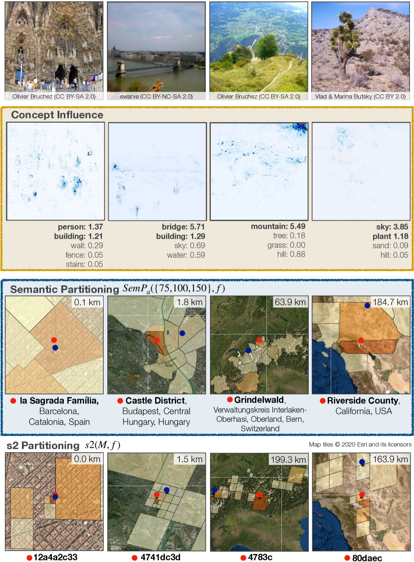
Figure 3: Output of the proposed concept influence metric in addition to the explanation map [38] and qualitative comparison of predictions from the $\text{\lx@glossaries@gls@link{main}{ah}{\leavevmode\emph{SemP}}}_{a}$ model and $s2(M,f)$ [21] (last two rows). The top-25 classes and probabilities are visualized on the zoomed world map. Below is the predicted class label whereas the red marker is the predicted coordinate (blue is ground-truth).

4.2 Understanding the Input Feature Importance

Table 3: The concept influence (ci${}_{\text{median}}$) aggregated for each visual concept ($s$) in YFCC-Val26k and binned into spatial intervals depending on the achieved GCD error in $km$. Presented are the highest and lowest $k=10$ concepts per spatial interval according to ci.

top-10									lowest-10
$[0-25)$			$[25-750)$			$[750-2500)$			$[0-25)$			$[25-750)$			$[750-2500)$
$s$	$|s|$	ci	$s$	$|s|$	ci	$s$	$|s|$	ci	$s$	$|s|$	ci	$s$	$|s|$	ci	$s$	$|s|$	ci
tower	58	1.51	windowpane	109	1.74	windowpane	119	2.13	floor	354	0.24	table	119	0.15	base	67	0.22
sky	2114	1.29	animal	142	1.4	animal	162	1.38	car	149	0.21	field	150	0.15	chair	70	0.19
animal	58	1.26	sky	2494	1.38	sky	1518	1.15	earth	486	0.16	path	54	0.14	sand	65	0.18
building	1851	1.13	house	92	1.3	person	2218	1.15	water	432	0.16	grass	761	0.12	grass	521	0.18
mountain	439	1.09	mountain	571	1.18	building	1083	1.1	plant	206	0.13	railing	61	0.12	field	78	0.17
windowpane	51	1.04	airplane	74	1.09	mountain	279	1.09	grass	380	0.11	bicycle	58	0.11	table	185	0.17
bridge	86	0.96	building	1658	1.06	airplane	53	1.09	sand	70	0.08	chair	66	0.09	bicycle	62	0.13
person	1223	0.79	person	2015	0.99	flower	103	1.06	field	66	0.08	road	620	0.08	seat	68	0.09
grandstand	61	0.79	flower	101	0.95	tree	1247	0.97	road	463	0.07	sand	114	0.08	sidewalk	198	0.09
wall	1092	0.74	tree	1889	0.9	painting	141	0.91	sidewalk	303	0.04	sidewalk	294	0.07	road	383	0.08

It is likely that certain visual concepts influence the predictions of a model differently at various geographical levels. For instance, for landmarks, architectural features are probably dominant, whereas for landscapes with few visual clues to a concrete location, vegetation may provide some cues for a rough estimate. To investigate the proposed ci score for several concepts on such geographic levels, we aggregate the ci score for each concept $s\in\mathbb{S}$. We examine three geographic levels, where we assume the model predicts the location correctly based on different geographic properties. In particular, we consider $[0-25)\,km$ for precisely predictable locations, $[25-750)\,km$ for regions, and $[750-2500)\,km$ for photos with few visual cues for a concrete location. These are strict intervals where, for instance, a photo with a GCD $<1\,km$ is not considered for the $[25-750)\,km$ interval. To aggregate the ci, we compute the median  ($ci_{\text{median}}$) and use it instead of the mean to ignore larger outlier(s). Please note, that similar conclusions can also be drawn from the mean value (see Appendix). According to its definition (Section 3.2), the ci score for concepts with geographic clues is expected to be greater than or equal to one, whereas the score for concepts without any hints should be close to zero.

Setup:

We apply the ci score to YFCC-Val26k due to its larger size compared to the test sets, and focus on the reproduced $s2(M,f^{*})$ model in this experiment. Since current segmentation models achieve high-quality results, we apply the HRNetV2 [37] which is trained on the ADE20k [47] dataset that contains 150 object classes (e.g., person, car, bottle) and concepts for scene parsing (e.g., sky, ground, mountain) and is therefore well suited. According to a study [12], the method of Integrated Gradients [38] is chosen as explanation method, extended by SmoothGrad [35] which seeks to alleviate noise in explanation maps. Inserting random Gaussian noise in $n$ copies of the input image and then averaging the produced explanation maps cleans up artifacts. The noise parameter is set to $\sigma=0.15$ as suggested by the authors, but the sample size is reduced from $20$ to $5$ due to computing complexity without major result changes. Please note, that the variant as in [12] is used which squares each value before averaging.

Influence of Individual Concepts:

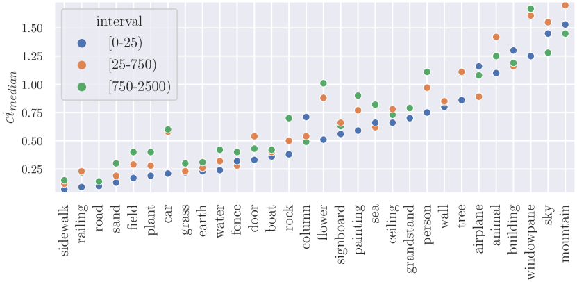
Figure 4: Absolute $ci_{\text{median}}$ scores for a selection of visual concepts divided in three geographic intervals.

We report results for the top-$k$ and lowest-$k$ ci scores, i.e., concept label, $ci_{\text{median}}$, and the number of concepts ($|s|$) that fall into the evaluation interval. Table 3 shows results for concepts that occur in at least 50 images and where the morphological dilation is set to $\beta=0$. The complete table containing all concepts can be found in the Appendix. Figure 4 shows the absolute $ci_{\text{median}}$ per concept for the respective geographic interval with a selection of concepts with high discrepancies. The following observations can be made from Table 3. Concepts like tower, building, bridge, or mountain have a high influence ($ci_{\text{median}}\gtrapprox 1$) at the $[0,25)\,km$ interval and correspond to expected concepts to locate a place more precisely. On the contrary, concepts like grass, road, water, or car have very limited influence ($ci_{\text{median}}\lessapprox 0.2$), which seems reasonable since these concepts are rather general concepts that are visually similar all over the world. The concept of sky has an initially surprisingly large influence on the prediction. The two examples in Figure 3 (last two images) indicate that architectural details of buildings or peaks of mountain ranges can be relevant, i.e., the sky-touching concepts. With the introduction of the morphological dilation ($m^{\beta}(\boldsymbol{x},s)$) this area is covered. A repetition of this experiment with the enlarged area ($\beta=3$) confirmed this assumption. Since the ci increases for windowpane, person, tree, or animal on higher geographical levels, such concepts are more relevant for rough estimations, where there are few visual clues to a more concrete location. Lastly, the examples in Figure 3 show an additional property of the presented metric for single instances. It does not determine the particular concept that is crucial for a prediction but rather which concepts are influential.

5 Conclusions

In this paper, we have presented a novel semantic photo geolocalization system that allows for the interpretation of results. To achieve this, we have proposed a semantic partitioning method that leads to an improved comprehensibility of predictions while at the same time achieving state-of-the-art results on common benchmark test sets. In addition, we have suggested a novel metric to assess the importance of semantic visual concepts for a certain prediction to provide additional explanatory information, and to allow for a large-scale analysis of already trained models.

In the future, we plan to incorporate visual similarities between classes based on geographical features during optimization, e.g., derived from a knowledge base, since currently visual and spatial proximate classes are equally penalized as visual and spatial dissimilar classes.

Appendix A Influence of Individual Concepts

A.1 Morphological Dilation $\beta$

As mentioned in the paper, the concept sky has an initially surprisingly large influence on the prediction. We argued that sky-touching concepts could be responsible for this as the boundaries between concepts are likely of interest for the model. To cover this area with the ci, we have introduced the morphological dilation ($m^{\beta}$(x, s). We compute the ci ${}_{\text{median}}$ both for $\beta=3\,px$ and $\beta=0\,px$ and those concepts, as $3\,px$ are sufficient to cover these boundaries. In Table 4 the absolute difference between ci ${}_{\text{median}}^{\beta=3}$ and ci ${}_{\text{median}}^{\beta=0}$ is reported. The significant increase for mountain and tower confirms our explanation. However, the same effect cannot be observed for building. The reason is that this concept covers a wide range of sub-concepts that are not investigated quantitatively in this work. However, we are confident that the same effect can be observed when sub-concepts like skyscraper or stadium are investigated individually as qualitative examples indicate this. With the release of source code we hope to foster further research in this area as we were only able to provide initial insights with the ci in this paper.

Table 4: The absolute difference $\Delta$ of the concept influence (ci${}_{\text{median}}$) for morphological dilation ($\beta=3$ and $\beta=0$) aggregated for relevant sky-touching concepts in YFCC-Val26k and binned into spatial intervals depending on the achieved GCD error in $km$.

concept	$\Delta_{\beta}$ $[0-25)$	$\Delta_{\beta}$ $[25-750)$	$\Delta_{\beta}$ $[750-2500)$
sky	+0.16	+0.17	+0.13
mountain	+0.44	+0.52	+0.36
building	+0.17	+0.10	+0.09
tower	+0.34	-	-

A.2 Aggregation Operator

To aggregate the ci score over all images for a certain concept, the median or average operator was suggested. In Table 5,6 both variants are reported for all concepts where at least ten images are available whereas only the top/last-k concepts were reported in the main paper with at least 50 images.

Table 5: The concept influence aggregated for each visual concept $s$ (start letter a-m) in YFCC-Val26k and binned into spatial intervals depending on the achieved GCD error in $km$. Presented are concepts of the dataset where at least 10 images are available.

	median			mean
	[0-25)	[25-750)	[750-2500)	[0-25)	[25-750)	[750-2500)
airplane	1.32	1.09	1.09	1.92	1.53	2.11
animal	1.26	1.40	1.38	2.20	2.11	2.02
apparel		0.15	0.12		0.29	0.23
armchair			0.22			0.34
awning	0.18	0.35	0.54	0.51	1.00	1.23
bag			0.20			0.67
ball		0.59	0.70		0.89	0.70
bannister	0.13	0.21		0.72	0.60
bar			0.51			0.85
barrel		0.18	0.37		0.74	0.61
base	0.37	0.40	0.22	0.70	0.78	0.68
bed		0.19	0.67		0.41	0.65
bicycle	0.11	0.11	0.13	0.41	0.54	0.57
boat	0.30	0.30	0.28	0.75	0.77	1.01
book			0.31			0.98
bottle		0.19	0.76		0.70	0.93
box	0.48	0.30	0.57	0.88	0.51	0.98
bridge	0.96	0.29	0.83	1.52	0.91	1.23
building	1.13	1.06	1.10	1.57	1.49	1.56
bulletin	0.73	0.33	0.44	0.89	0.96	0.49
bus	0.69	0.82	0.89	0.86	1.25	0.75
cabinet		0.28	0.49		0.70	1.21
car	0.21	0.54	0.52	0.79	0.97	0.89
case			0.18			0.55
ceiling	0.61	0.68	0.59	1.10	1.21	0.95
chair	0.09	0.09	0.19	0.79	0.46	0.52
clock		0.35	0.89		0.53	1.30
column	0.71	0.45	0.25	0.91	1.26	0.83
computer			0.29			0.68
counter			0.29			0.95
crt	0.85	1.40	0.48	1.42	1.13	0.94
curtain	0.25	0.37	0.30	0.52	0.84	0.80
desk		0.53	0.21		0.75	0.63
dirt	0.04	0.03	0.03	0.25	0.10	0.11
door	0.27	0.47	0.30	0.85	0.77	0.77
earth	0.16	0.17	0.22	0.47	0.50	0.55
fence	0.24	0.17	0.32	0.73	0.62	0.72
field	0.08	0.15	0.17	0.35	0.49	0.64
floor	0.24	0.20	0.29	0.67	0.54	0.61
flower	0.46	0.95	1.06	1.14	1.39	1.22
food	0.93	0.66	0.62	1.30	1.00	0.84
fountain	0.39	0.78	0.25	1.06	1.29	0.82
grandstand	0.79	1.02	0.86	1.01	1.22	1.09
grass	0.11	0.12	0.18	0.41	0.44	0.52
hill	0.47	0.44	0.68	1.05	1.05	1.05
house	1.98	1.30	1.29	1.92	1.85	1.48
hovel		0.77	0.63		1.30	1.39
land		0.77			1.67
minibike	0.36	0.63	0.15	0.91	0.95	0.52
mountain	1.09	1.18	1.09	1.72	1.82	1.67

Table 6: The concept influence aggregated for each visual concept $s$ (start letter n-z) in YFCC-Val26k and binned into spatial intervals depending on the achieved GCD error in $km$. Presented are concepts of the dataset where at least 10 images are available.

	median			mean
	[0-25)	[25-750)	[750-2500)	[0-25)	[25-750)	[750-2500)
painting	0.52	0.78	0.91	0.82	0.96	1.14
palm	0.67	0.72	1.12	1.09	1.84	1.69
path	0.10	0.14	0.09	0.62	0.87	0.76
person	0.79	0.99	1.15	1.17	1.33	1.45
pier	0.09	0.05		0.44	0.42
plant	0.13	0.24	0.38	0.49	0.57	0.66
plate		0.83	0.54		1.30	0.81
plaything		0.55	0.45		1.50	1.18
pole	0.02	0.19		0.31	0.46
poster		0.58	0.47		1.33	1.53
railing	0.11	0.12	0.13	0.42	0.53	0.47
river	0.10	0.07	0.10	0.49	0.33	0.54
road	0.07	0.08	0.08	0.30	0.40	0.37
rock	0.37	0.49	0.67	0.86	1.05	1.24
runway	0.15	0.28	0.15	0.37	0.54	0.38
sand	0.08	0.08	0.18	0.36	0.45	0.67
sculpture	0.58	0.68	0.58	1.44	0.92	1.14
sea	0.40	0.32	0.49	0.86	0.84	0.91
seat	0.18	0.25	0.09	0.50	0.50	0.35
shelf		0.43	0.69		1.00	0.87
ship	0.50	0.81	0.60	1.12	1.03	0.93
sidewalk	0.04	0.07	0.09	0.31	0.51	0.40
signboard	0.60	0.64	0.57	1.27	1.31	1.26
sink		1.05	0.97		1.09	1.04
sky	1.29	1.38	1.15	1.96	2.08	1.78
skyscraper	0.30			0.72
sofa			0.22			0.43
stage	0.62	0.31	1.19	1.15	0.55	1.41
stairs	0.03	0.05	0.21	0.21	0.31	0.51
stairway	0.13	0.13	0.17	0.41	0.64	0.39
table	0.17	0.15	0.17	0.67	0.53	0.63
tank		0.41	0.48		0.56	0.72
tent	1.13	0.25	0.40	1.51	0.78	0.84
tower	1.51	0.73	1.58	2.21	1.15	2.27
tray		0.61	0.55		0.90	0.95
tree	0.71	0.90	0.97	1.25	1.43	1.53
truck	0.75	0.65	0.92	0.94	1.04	1.13
van			0.49			0.82
wall	0.74	0.78	0.78	0.92	0.98	0.98
water	0.16	0.21	0.33	0.48	0.57	0.58
waterfall	0.87	0.38	0.50	2.18	0.99	0.93
windowpane	1.04	1.74	2.13	2.28	2.63	2.75

Appendix B Extended MP-16 Dataset (EMP-16)

Assigning a single GPS coordinate to each type of image is debatable in terms of content, but corresponds to the traditional task where one image is assigned to exactly one coordinate. At present, even specialized models struggle because of the complexity of the task, making a discretization of coordinates with semantic context necessary in our opinion.

As formally described in the main paper, a reverse geocoder can be used to assign each coordinate an address, which is our required information to construct the semantic partitioning (SemP). Thanks to OSM many additional information (e.g. geometry) are available for each location of an address. To foster future research in this context, we extend the MediaEval Placing Task 2016 (MP-16) [16] dataset for photo geolocalization (image-coordinate pairs) with those additional information and call it Extended MP-16 (EMP-16). This section provides a short insight of the construction and resulting dataset.

As described in the paper, we utilize the MP-16 [16] dataset that is a subset from the Yahoo Flickr Creative Commons 100 Million (YFCC100M) [40]. Its only restriction is that an image contains a GPS coordinate, thus it contains images of landmarks, landscape images, but also images with little to no geographical cues. Like Vo et al. [43] images are excluded from the same authors as in the Im2GPS3k test set and duplicates are removed resulting in a dataset size of 4,723,695 image-coordinate pairs.

Table 7: Example for additional meta-information available for extracted locations from OSM: Given the GPS coordinate of an image-coordinate pair, each location of the resulting address hierarchy (e.g. [W438331516, W13470104, …]) contains additional context information. Geometry contains single points, multi-lines, polygons and multi-polygons.

id	W438331516	W13470104	R112100	R396479	R165475	R148838
localname	The Queen Mary	Windsor Way	Long Beach	Los Angeles County	California	United States
category	historic	highway	boundary	boundary	boundary	boundary
type	ship	service	administrative	administrative	administrative	administrative
admin_level	15	15	8	6	4	2
isarea	True	False	True	True	True	True
wikidata	Q752939	NA	Q16739	Q104994	Q99	Q30
wikipedia	NA	NA	en:Long Beach, California	en:Los Angeles County, California	en:California	en:United States
population	NA	NA	469450	NA	37253956	324720797
place	NA	NA	city	county	state	country
geometry	[[[-118.191…	[[-118.1…	[[[-118.248…	[[[[-1…	[[[[-1…	[[[[-1…

For reverse geocoding we have applied Nominatim v3.4 on a planet-scale OSM installation with a dump from 22nd May 2020. After initial reverse geocoding and ignoring postal codes, the resulting multi-label dataset contains 1,191,616 unique locations which is not useful for this dataset size. To reduce the number, an initial filtering step with $\tau_{\mathbb{D}}=50$ is applied that removes non-frequent locations resulting in manageable 46,240 unique locations. Each unique location which is identified by osm_type amd osm_id has a set of additional attributes such as localname, geometry or sometimes even links to the wikidata [44] knowledge base. The extended information for one sample (image-coordinate pair) of the MP-16 dataset is presented in Table 7. Since only the ids, localnames and available geometry are used in this work, a full description and statistics of available attributes goes beyond of the scope of this paper.

Appendix C Model Pre-Training

It was mentioned that the initial weights from all trained models are not selected randomly or taken from a model that was trained on ImageNet [28] as commonly chosen, but with weights of a pre-trained model which already learned geo-related features to reduce the training time. This sections provides missing details about the weight initialization.

Task and Data:

To construct a simple geolocation classification problem, each image is associated with the country (including maritime borders) the image was taken. Note, that an image is associated to its country by checking whether its respective coordinate is within the area that the country covers and no function of the method presented in Section 3 like Reverse Geocoding is applied. As data basis serves the MP-16 [16] dataset for training and YFCC-Val26k for validation. Due to class imbalance, the USA is divided into individual states and a country is only considered if there are at least 1,000 images for training which results in 173 classes in total.

Network Training and Results:

One ResNet-50 is initialized with ImageNet weights and optimized using the SGDR [20] method with weight decay of $10^{-4}$, a momentum of $0.9$, a maximum learning rate of $5\times 10^{-3}$ and one cycle is performed three times per epoch. The model is trained for ten epochs and is validated every 4,000 steps for a batch size of 128 (512,000 images). The same image pre-processing and data augmentation methods are applied as described in the paper and below. The standard classification loss (cross-entropy) is used as loss function, i.e. one-hot-encoded vectors as ground-truth class) and the best model on the validation set is selected. After training, this trained model achieves a top-1 accuracy of 0.24 percent (0.49 top-5).

Appendix D Image Augmentation

During training, images are augmented as follows to prevent overfitting: Images are initially resized to a minimum edge size of 320 pixels. After that, we crop a region of random size (between $0.66$ and $1.0$ of original size) and random aspect ratio (3/4 to 4/3) of the original aspect ratio. This crop is finally resized to $224\times 224$ pixels ($300\times 300$ for EfficientNet) and randomly flipped horizontally. For validation, the image is resized to a minimum edge size of $256$ ($320$) pixels and then a center crop of size $224$ ($300$) pixels is made.

References

- Ancona et al. [2017] Marco Ancona, Enea Ceolini, A. Cengiz Öztireli, and Markus H. Gross. A unified view of gradient-based attribution methods for deep neural networks. CoRR, abs/1711.06104, 2017.
- Arandjelovic et al. [2018] Relja Arandjelovic, Petr Gronát, Akihiko Torii, Tomás Pajdla, and Josef Sivic. Netvlad: CNN architecture for weakly supervised place recognition. IEEE Trans. Pattern Anal. Mach. Intell., 40(6):1437–1451, 2018.
- Baatz et al. [2012] Georges Baatz, Olivier Saurer, Kevin Köser, and Marc Pollefeys. Large scale visual geo-localization of images in mountainous terrain. In Andrew W. Fitzgibbon, Svetlana Lazebnik, Pietro Perona, Yoichi Sato, and Cordelia Schmid, editors, Computer Vision - ECCV 2012 - 12th European Conference on Computer Vision, Florence, Italy, October 7-13, 2012, Proceedings, Part II, volume 7573 of Lecture Notes in Computer Science, pages 517–530. Springer, 2012.
- Ghorbani et al. [2019] Amirata Ghorbani, Abubakar Abid, and James Y. Zou. Interpretation of neural networks is fragile. In The Thirty-Third AAAI Conference on Artificial Intelligence, AAAI 2019, The Thirty-First Innovative Applications of Artificial Intelligence Conference, IAAI 2019, The Ninth AAAI Symposium on Educational Advances in Artificial Intelligence, EAAI 2019, Honolulu, Hawaii, USA, January 27 - February 1, 2019, pages 3681–3688. AAAI Press, 2019.
- Gilpin et al. [2018] Leilani H. Gilpin, David Bau, Ben Z. Yuan, Ayesha Bajwa, Michael Specter, and Lalana Kagal. Explaining explanations: An overview of interpretability of machine learning. In Francesco Bonchi, Foster J. Provost, Tina Eliassi-Rad, Wei Wang, Ciro Cattuto, and Rayid Ghani, editors, 5th IEEE International Conference on Data Science and Advanced Analytics, DSAA 2018, Turin, Italy, October 1-3, 2018, pages 80–89. IEEE, 2018.
- Gordo et al. [2016] Albert Gordo, Jon Almazán, Jérôme Revaud, and Diane Larlus. Deep image retrieval: Learning global representations for image search. In Bastian Leibe, Jiri Matas, Nicu Sebe, and Max Welling, editors, Computer Vision - ECCV 2016 - 14th European Conference, Amsterdam, The Netherlands, October 11-14, 2016, Proceedings, Part VI, volume 9910 of Lecture Notes in Computer Science, pages 241–257. Springer, 2016.
- Guidotti et al. [2019] Riccardo Guidotti, Anna Monreale, Salvatore Ruggieri, Franco Turini, Fosca Giannotti, and Dino Pedreschi. A survey of methods for explaining black box models. ACM Comput. Surv., 51(5):93:1–93:42, 2019.
- Hays and Efros [2008] James Hays and Alexei A. Efros. IM2GPS: estimating geographic information from a single image. In 2008 IEEE Computer Society Conference on Computer Vision and Pattern Recognition (CVPR 2008), 24-26 June 2008, Anchorage, Alaska, USA. IEEE Computer Society, 2008.
- Hays and Efros [2015] James Hays and Alexei A. Efros. Large-scale image geolocalization. In Jaeyoung Choi and Gerald Friedland, editors, Multimodal Location Estimation of Videos and Images, pages 41–62. Springer, 2015.
- He et al. [2016] Kaiming He, Xiangyu Zhang, Shaoqing Ren, and Jian Sun. Deep residual learning for image recognition. In 2016 IEEE Conference on Computer Vision and Pattern Recognition, CVPR 2016, Las Vegas, NV, USA, June 27-30, 2016, pages 770–778. IEEE Computer Society, 2016.
- He et al. [2016] Kaiming He, Xiangyu Zhang, Shaoqing Ren, and Jian Sun. Identity mappings in deep residual networks. In Bastian Leibe, Jiri Matas, Nicu Sebe, and Max Welling, editors, Computer Vision - ECCV 2016 - 14th European Conference, Amsterdam, The Netherlands, October 11-14, 2016, Proceedings, Part IV, volume 9908 of Lecture Notes in Computer Science, pages 630–645. Springer, 2016.
- Hooker et al. [2019] Sara Hooker, Dumitru Erhan, Pieter-Jan Kindermans, and Been Kim. A benchmark for interpretability methods in deep neural networks. In Hanna M. Wallach, Hugo Larochelle, Alina Beygelzimer, Florence d’Alché-Buc, Emily B. Fox, and Roman Garnett, editors, Advances in Neural Information Processing Systems 32: Annual Conference on Neural Information Processing Systems 2019, NeurIPS 2019, 8-14 December 2019, Vancouver, BC, Canada, pages 9734–9745, 2019.
- Izbicki et al. [2019] Mike Izbicki, Evangelos E. Papalexakis, and Vassilis J. Tsotras. Exploiting the earth’s spherical geometry to geolocate images. In Ulf Brefeld, Élisa Fromont, Andreas Hotho, Arno J. Knobbe, Marloes H. Maathuis, and Céline Robardet, editors, Machine Learning and Knowledge Discovery in Databases - European Conference, ECML PKDD 2019, Würzburg, Germany, September 16-20, 2019, Proceedings, Part II, volume 11907 of Lecture Notes in Computer Science, pages 3–19. Springer, 2019.
- Jégou et al. [2008] Hervé Jégou, Matthijs Douze, and Cordelia Schmid. Hamming embedding and weak geometric consistency for large scale image search. In David A. Forsyth, Philip H. S. Torr, and Andrew Zisserman, editors, Computer Vision - ECCV 2008, 10th European Conference on Computer Vision, Marseille, France, October 12-18, 2008, Proceedings, Part I, volume 5302 of Lecture Notes in Computer Science, pages 304–317. Springer, 2008.
- Kordopatis-Zilos et al. [2021] Giorgos Kordopatis-Zilos, Panagiotis Galopoulos, Symeon Papadopoulos, and Ioannis Kompatsiaris. Leveraging efficientnet and contrastive learning for accurate global-scale location estimation. In Wen-Huang Cheng, Mohan S. Kankanhalli, Meng Wang, Wei-Ta Chu, Jiaying Liu, and Marcel Worring, editors, ICMR ’21: International Conference on Multimedia Retrieval, Taipei, Taiwan, August 21-24, 2021, pages 155–163. ACM, 2021.
- Larson et al. [2017] Martha A. Larson, Mohammad Soleymani, Guillaume Gravier, Bogdan Ionescu, and Gareth J. F. Jones. The benchmarking initiative for multimedia evaluation: Mediaeval 2016. IEEE Multim., 24(1):93–96, 2017.
- Lee et al. [2015] Stefan Lee, Haipeng Zhang, and David J. Crandall. Predicting geo-informative attributes in large-scale image collections using convolutional neural networks. In 2015 IEEE Winter Conference on Applications of Computer Vision, WACV 2015, Waikoloa, HI, USA, January 5-9, 2015, pages 550–557. IEEE Computer Society, 2015.
- Lin et al. [2013] Tsung-Yi Lin, Serge J. Belongie, and James Hays. Cross-view image geolocalization. In 2013 IEEE Conference on Computer Vision and Pattern Recognition, Portland, OR, USA, June 23-28, 2013, pages 891–898. IEEE Computer Society, 2013.
- Liu et al. [2019] Liu Liu, Hongdong Li, and Yuchao Dai. Stochastic attraction-repulsion embedding for large scale image localization. In 2019 IEEE/CVF International Conference on Computer Vision, ICCV 2019, Seoul, Korea (South), October 27 - November 2, 2019, pages 2570–2579. IEEE, 2019.
- Loshchilov and Hutter [2017] Ilya Loshchilov and Frank Hutter. SGDR: stochastic gradient descent with warm restarts. In 5th International Conference on Learning Representations, ICLR 2017, Toulon, France, April 24-26, 2017, Conference Track Proceedings. OpenReview.net, 2017.
- Müller-Budack et al. [2018] Eric Müller-Budack, Kader Pustu-Iren, and Ralph Ewerth. Geolocation estimation of photos using a hierarchical model and scene classification. In Vittorio Ferrari, Martial Hebert, Cristian Sminchisescu, and Yair Weiss, editors, Computer Vision - ECCV 2018 - 15th European Conference, Munich, Germany, September 8-14, 2018, Proceedings, Part XII, volume 11216 of Lecture Notes in Computer Science, pages 575–592. Springer, 2018.
- Noh et al. [2017] Hyeonwoo Noh, Andre Araujo, Jack Sim, Tobias Weyand, and Bohyung Han. Large-scale image retrieval with attentive deep local features. In IEEE International Conference on Computer Vision, ICCV 2017, Venice, Italy, October 22-29, 2017, pages 3476–3485. IEEE Computer Society, 2017.
- [23] Nominatim. https://https://nominatim.org/. Accessed: 2020-11-14.
- OpenStreetMap contributors [2017] OpenStreetMap contributors. Planet dump retrieved from https://planet.osm.org. https://www.openstreetmap.org, 2017.
- Philbin et al. [2007] James Philbin, Ondrej Chum, Michael Isard, Josef Sivic, and Andrew Zisserman. Object retrieval with large vocabularies and fast spatial matching. In 2007 IEEE Computer Society Conference on Computer Vision and Pattern Recognition (CVPR 2007), 18-23 June 2007, Minneapolis, Minnesota, USA. IEEE Computer Society, 2007.
- Philbin et al. [2008] James Philbin, Ondrej Chum, Michael Isard, Josef Sivic, and Andrew Zisserman. Lost in quantization: Improving particular object retrieval in large scale image databases. In 2008 IEEE Computer Society Conference on Computer Vision and Pattern Recognition (CVPR 2008), 24-26 June 2008, Anchorage, Alaska, USA. IEEE Computer Society, 2008.
- Radenovic et al. [2016] Filip Radenovic, Giorgos Tolias, and Ondrej Chum. CNN image retrieval learns from bow: Unsupervised fine-tuning with hard examples. In Bastian Leibe, Jiri Matas, Nicu Sebe, and Max Welling, editors, Computer Vision - ECCV 2016 - 14th European Conference, Amsterdam, The Netherlands, October 11-14, 2016, Proceedings, Part I, volume 9905 of Lecture Notes in Computer Science, pages 3–20. Springer, 2016.
- Russakovsky et al. [2015] Olga Russakovsky, Jia Deng, Hao Su, Jonathan Krause, Sanjeev Satheesh, Sean Ma, Zhiheng Huang, Andrej Karpathy, Aditya Khosla, Michael S. Bernstein, Alexander C. Berg, and Fei-Fei Li. Imagenet large scale visual recognition challenge. Int. J. Comput. Vis., 115(3):211–252, 2015.
- [29] S2library. https://s2geometry.io/. Accessed: 2020-11-14.
- Sattler et al. [2016] Torsten Sattler, Michal Havlena, Konrad Schindler, and Marc Pollefeys. Large-scale location recognition and the geometric burstiness problem. In 2016 IEEE Conference on Computer Vision and Pattern Recognition, CVPR 2016, Las Vegas, NV, USA, June 27-30, 2016, pages 1582–1590. IEEE Computer Society, 2016.
- Saurer et al. [2016] Olivier Saurer, Georges Baatz, Kevin Köser, Lubor Ladicky, and Marc Pollefeys. Image based geo-localization in the alps. Int. J. Comput. Vis., 116(3):213–225, 2016.
- Schindler et al. [2007] Grant Schindler, Matthew A. Brown, and Richard Szeliski. City-scale location recognition. In 2007 IEEE Computer Society Conference on Computer Vision and Pattern Recognition (CVPR 2007), 18-23 June 2007, Minneapolis, Minnesota, USA. IEEE Computer Society, 2007.
- Seo et al. [2018] Paul Hongsuck Seo, Tobias Weyand, Jack Sim, and Bohyung Han. Cplanet: Enhancing image geolocalization by combinatorial partitioning of maps. In Vittorio Ferrari, Martial Hebert, Cristian Sminchisescu, and Yair Weiss, editors, Computer Vision - ECCV 2018 - 15th European Conference, Munich, Germany, September 8-14, 2018, Proceedings, Part X, volume 11214 of Lecture Notes in Computer Science, pages 544–560. Springer, 2018.
- Simonyan et al. [2014] Karen Simonyan, Andrea Vedaldi, and Andrew Zisserman. Deep inside convolutional networks: Visualising image classification models and saliency maps. In Yoshua Bengio and Yann LeCun, editors, 2nd International Conference on Learning Representations, ICLR 2014, Banff, AB, Canada, April 14-16, 2014, Workshop Track Proceedings, 2014.
- Smilkov et al. [2017] Daniel Smilkov, Nikhil Thorat, Been Kim, Fernanda B. Viégas, and Martin Wattenberg. Smoothgrad: removing noise by adding noise. CoRR, abs/1706.03825, 2017.
- Springenberg et al. [2015] Jost Tobias Springenberg, Alexey Dosovitskiy, Thomas Brox, and Martin A. Riedmiller. Striving for simplicity: The all convolutional net. In Yoshua Bengio and Yann LeCun, editors, 3rd International Conference on Learning Representations, ICLR 2015, San Diego, CA, USA, May 7-9, 2015, Workshop Track Proceedings, 2015.
- Sun et al. [2019] Ke Sun, Yang Zhao, Borui Jiang, Tianheng Cheng, Bin Xiao, Dong Liu, Yadong Mu, Xinggang Wang, Wenyu Liu, and Jingdong Wang. High-resolution representations for labeling pixels and regions. CoRR, abs/1904.04514, 2019.
- Sundararajan et al. [2017] Mukund Sundararajan, Ankur Taly, and Qiqi Yan. Axiomatic attribution for deep networks. In Doina Precup and Yee Whye Teh, editors, Proceedings of the 34th International Conference on Machine Learning, ICML 2017, Sydney, NSW, Australia, 6-11 August 2017, volume 70 of Proceedings of Machine Learning Research, pages 3319–3328. PMLR, 2017.
- Tan and Le [2019] Mingxing Tan and Quoc Le. Efficientnet: Rethinking model scaling for convolutional neural networks. In International Conference on Machine Learning, pages 6105–6114. PMLR, 2019.
- Thomee et al. [2016] Bart Thomee, David A. Shamma, Gerald Friedland, Benjamin Elizalde, Karl Ni, Douglas Poland, Damian Borth, and Li-Jia Li. YFCC100M: the new data in multimedia research. Commun. ACM, 59(2):64–73, 2016.
- Tolias et al. [2016] Giorgos Tolias, Ronan Sicre, and Hervé Jégou. Particular object retrieval with integral max-pooling of CNN activations. In Yoshua Bengio and Yann LeCun, editors, 4th International Conference on Learning Representations, ICLR 2016, San Juan, Puerto Rico, May 2-4, 2016, Conference Track Proceedings, 2016.
- Tzeng et al. [2013] Eric Tzeng, Andrew Zhai, Matthew Clements, Raphael Townshend, and Avideh Zakhor. User-driven geolocation of untagged desert imagery using digital elevation models. In IEEE Conference on Computer Vision and Pattern Recognition, CVPR Workshops 2013, Portland, OR, USA, June 23-28, 2013, pages 237–244. IEEE Computer Society, 2013.
- Vo et al. [2017] Nam N. Vo, Nathan Jacobs, and James Hays. Revisiting IM2GPS in the deep learning era. In IEEE International Conference on Computer Vision, ICCV 2017, Venice, Italy, October 22-29, 2017, pages 2640–2649. IEEE Computer Society, 2017.
- Vrandečić and Krötzsch [2014] Denny Vrandečić and Markus Krötzsch. Wikidata: a free collaborative knowledgebase. Communications of the ACM, 57(10):78–85, 2014.
- Weyand et al. [2016] Tobias Weyand, Ilya Kostrikov, and James Philbin. Planet - photo geolocation with convolutional neural networks. In Bastian Leibe, Jiri Matas, Nicu Sebe, and Max Welling, editors, Computer Vision - ECCV 2016 - 14th European Conference, Amsterdam, The Netherlands, October 11-14, 2016, Proceedings, Part VIII, volume 9912 of Lecture Notes in Computer Science, pages 37–55. Springer, 2016.
- Zheng et al. [2009] Yantao Zheng, Ming Zhao, Yang Song, Hartwig Adam, Ulrich Buddemeier, Alessandro Bissacco, Fernando Brucher, Tat-Seng Chua, and Hartmut Neven. Tour the world: Building a web-scale landmark recognition engine. In 2009 IEEE Computer Society Conference on Computer Vision and Pattern Recognition (CVPR 2009), 20-25 June 2009, Miami, Florida, USA, pages 1085–1092. IEEE Computer Society, 2009.
- Zhou et al. [2017] Bolei Zhou, Hang Zhao, Xavier Puig, Sanja Fidler, Adela Barriuso, and Antonio Torralba. Scene parsing through ADE20K dataset. In 2017 IEEE Conference on Computer Vision and Pattern Recognition, CVPR 2017, Honolulu, HI, USA, July 21-26, 2017, pages 5122–5130. IEEE Computer Society, 2017.