Passive soft-reset controllers for nonlinear systems

Abstract

Soft-reset controllers are introduced as a way to approximate hard-reset controllers. The focus is on implementing reset controllers that are (strictly) passive and on analyzing their interconnection with passive plants. A passive hard-reset controller that has a strongly convex energy function can be approximated as a soft-reset controller. A hard-reset controller is a hybrid system whereas a soft-reset controller corresponds to a differential inclusion, living entirely in the continuous-time domain. This feature may make soft-reset controllers easier to understand and implement. A soft-reset controller contains a parameter that can be adjusted to better approximate the action of the hard-reset controller. Closed-loop asymptotic stability is established for the interconnection of a passive soft-reset controller with a passive plant, under appropriate detectability assumptions. Several examples are used to illustrate the efficacy of soft-reset controllers.

I Introduction

A reset controller is a dynamical system whose state jumps to a new value when a prescribed condition, involving controller states and plant states, is realized. One of the earliest known reset controllers is due to Clegg, who introduced an integrating circuit that, for all intents and purposes, resets its state to zero when the product of the input and the output of the integrator attempts to become negative [1]. The Clegg integrator was extended by Horowitz and co-authors some twenty years later to more general “first-order reset elements” (FOREs) [2], [3]. After another two decades, stability and performance results for linear reset control systems began to receive significant attention, starting with the work of Hollot and co-authors [4], [5], [6], [7], [8], [9]. This work was continued and expanded upon within the hybrid systems framework of [10] in [11] and [12] for example. Other contributions pertaining to linear reset control systems include [13] and [14]. See [15] for a recent overview, perspective, and applications of linear reset control systems. For nonlinear reset control systems, Haddad and co-authors made noteworthy contributions, especially for lossless interconnections [16], [17] using an alternative hybrid systems framework [18]. In all of this work, controller resets are typically triggered by the closed-loop system state hitting a surface or attempting to enter a sector. Other reset control system mechanisms include those found in event-triggered control, where a control signal is typically held constant until a change to its value is required to maintain closed-loop stability or other properties [19], [20].

In this work, we consider an alternative implementation of control systems with resets triggered by the closed-loop system state attempting to enter a sector. We give conditions under which such a reset control system can be implemented using a differential inclusion rather than a hybrid system that involves resets. (Differential inclusions have appeared in other works related to reset control systems, including [21], [22], and [23].) We focus on nonlinear control problems, especially those where passivity plays a role, both in characterizing a nonlinear plant and also in characterizing a reset controller. Our results are inspired by similar results for linear reset control systems given in [24]. In Section III, we specify the passive, hard-reset controllers that we aim to implement as soft-reset controllers. We emphasize that such passive hard-reset controllers should admit a strongly convex energy function in order to be implementable as a soft-reset controller. Our passive soft-reset controllers are introduced in Section IV. In Section V, we discuss the interconnection of a passive soft-reset controller with a passive plant. Section VI contains several illustrations of the developed theory.

II Notation

For $x\in\mathbb{R}^{n}$, we use $|x|:=\sqrt{x^{T}x}$. Given a pair $(x,u)\in\mathbb{R}^{n}\times\mathbb{R}^{m}$, by abuse of notation we sometimes consider $z:=(x,u)$ to be a vector in $\mathbb{R}^{n+m}$. By the same abuse of notation, we sometimes write a function defined on $\mathbb{R}^{n}\times\mathbb{R}^{m}$ as a function defined on $\mathbb{R}^{n+m}$, i.e., $f(x,u)$ may be written as $f(z)$ with $z=(x,u)$. A function $f:\mathbb{R}^{n}\rightarrow\mathbb{R}^{m}$ is said to be sector bounded near the origin if there exist $\delta>0$ and $L>0$ such that $|f(z)|\leq L|z|$ for all $z\in\mathbb{R}^{n}$ satisfying $|z|\leq\delta$. It is said to be quadratically bounded near the origin if there exist $\delta>0$ and $L>0$ such that $|f(z)|\leq L|z|^{2}$ for all $z\in\mathbb{R}^{n}$ satisfying $|z|\leq\delta$. A function $V:\mathbb{R}^{n}\rightarrow\mathbb{R}$ is said to be convex if

$$V\left(\lambda x_{1}+(1-\lambda)x_{2}\right)\leq\lambda V(x_{1})+(1-\lambda)V(x_{2})$$

for all $x_{1},x_{2}\in\mathbb{R}^{n}$ and all $\lambda\in\left[0,1\right]$. It is said to be strongly convex if there exists $\mu>0$ such that $x\mapsto V(x)-\mu|x|^{2}$ is convex. A continuously differentiable function $V:\mathbb{R}^{n}\rightarrow\mathbb{R}$ is strongly convex if and only if there exists $\mu>0$ such that, for all $x,y\in\mathbb{R}^{n}$,

$$V(y)\geq V(x)+\langle\nabla V(x),y-x\rangle+\mu|x-y|^{2}.$$ (1)

III Passive hard-reset controllers

A (square) hard-reset control system is a hybrid system with state $x_{c}\in\mathbb{R}^{n_{c}}$, input $u_{c}\in\mathbb{R}^{m_{c}}$, and output $y_{c}\in\mathbb{R}^{m_{c}}$ with the following model:

$$(x_{c},u_{c}) \in C\qquad\dot{x}_{c}=f_{c}(x_{c},u_{c})$$ (2a)

$$(x_{c},u_{c}) \in D\qquad x_{c}^{+}=g_{c}(x_{c},u_{c})$$ (2b)

$$y_{c}=h_{c}(x_{c},u_{c})$$ (2c)

where, typically,

$$C :=\left\{(x_{c},u_{c})\in\mathbb{R}^{n_{c}}\times\mathbb{R}^{m_{c}}:\varphi(x_{c},u_{c})\leq 0\right\}$$ (3a)

$$D :=\left\{(x_{c},u_{c})\in\mathbb{R}^{n_{c}}\times\mathbb{R}^{m_{c}}:\varphi(x_{c},u_{c})\geq 0\right\}.$$ (3b)

We impose the following assumptions on the functions that prescribe the model.

Assumption 1

The following conditions hold for the functions $f_{c},g_{c},h_{c}$, and $\varphi$ that appear in (2)-(3):

1. (Continuous, locally sector bounded data and quadratic jump condition)
   There exists $M=M^{T}$ such that $\varphi(z_{c})=z_{c}^{T}Mz_{c}$ for all $z_{c}\in\mathbb{R}^{n_{c}+m_{c}}$; also, $f_{c}$, $g_{c}$, and $h_{c}$ are sector bounded near the origin and continuous.

2. (Jumps land in flow set)
   $(x_{c},u_{c})\in D$ implies $(g_{c}(x_{c},u_{c}),u_{c})\in C$.

3. (Passivity via a strongly convex energy function)
   There exist a strongly convex, positive definite, continuously differentiable function $V_{c}:\mathbb{R}^{n_{c}}\rightarrow\mathbb{R}_{\geq 0}$, a continuous, positive definite, quadratically bounded near the origin function $\rho:\mathbb{R}^{m_{c}}\rightarrow\mathbb{R}_{\geq 0}$, and $\varepsilon>0$ such that, with the definition

   $$C_{\varepsilon}:=\left\{z_{c}\in\mathbb{R}^{n_{c}+m_{c}}:z_{c}^{T}Mz_{c}\leq\varepsilon z_{c}^{T}z_{c}\right\},$$ (4)

   we have

   $$\langle\nabla V_{c}(x_{c}),\!f_{c}(x_{c},u_{c})\rangle \leq y_{c}^{T}u_{c}\!-\!\rho(y_{c})\ \ \forall(x_{c},u_{c})\in C_{\varepsilon}$$ (5a)

   $$V_{c}(g_{c}(x_{c},u_{c})) \leq V_{c}(x_{c})\qquad\quad\forall(x_{c},u_{c})\in D$$ (5b)

   where $y_{c}=h_{c}(x_{c},u_{c})$.

4. (Minimum phase and detectable)
   Any absolutely continuous, bounded solution $(x_{c},u_{c}):[0,\infty)\rightarrow\mathbb{R}^{n_{c}}\times\mathbb{R}^{m_{c}}$ of (2a), i.e., for almost all $t\in[0,\infty)$,

   $$(x_{c}(t),u_{c}(t))\in C,\quad\dot{x}_{c}(t)=f_{c}(x_{c}(t),u_{c}(t)),$$ (6)

   that satisfies $y_{c}(t)=0$ for all $t\in[0,\infty)$ also satisfies $\lim_{t\rightarrow\infty}u_{c}(t)=0$ and $\lim_{t\rightarrow\infty}x_{c}(t)=0$. $\blacksquare$

Assumption 1.2 implies that, after a jump, the solution of the hard-reset system (2)-(3) has the potential to flow without immediately jumping again. However, it is possible that $(g_{c}(x_{c},u_{c}),u_{c})\in C\cap D$, in which case the solution also has the potential to jump immediately. That is, there is no guarantee that all of the complete solutions of the hard-reset control system (2)-(3) have time domains that are unbounded in the ordinary time direction. This is one of the primary motivations for considering a “soft” implementation of the reset control system (2)-(3), as we do in the next section.

The crux of Assumption 1 is Assumption 1.3, which imposes a type of strict passivity condition on the hard-reset control system (2)-(3). For more context, compare with Assumption 2.2, where strict passivity of a continuous-time, passive plant is characterized. In addition, we use (5b) and the strong convexity of $V_{c}$ in the next section to propose the soft-reset implementation of the hard-reset system (2).

The following example illustrates a class of systems satisfying Assumption 1.

Example 1

Consider a hard-reset control system (2)-(3) with $(x_{c},u_{c})\in\mathbb{R}\times\mathbb{R}$, the following data:

$$f_{c}(x_{c},u_{c}) :=a_{c}x_{c}+b_{c}u_{c}$$ (7a)

$$g_{c}(x_{c},u_{c}) :=r_{c}x_{c}+p_{c}u_{c}$$ (7b)

$$h_{c}(x_{c},u_{c}) :=c_{c}x_{c}+d_{c}u_{c}$$ (7c)

$$M :=\left[\begin{array}[]{cc}m_{11}&m_{12}\\ m_{12}&m_{22}\end{array}\right]$$ (7f)

and the energy function

$$V_{c}(x_{c}):=\kappa x_{c}^{2}$$ (8)

where $\kappa>0$. There are no assumptions yet on the signs of the parameters in (7). Define

$$M_{0}:=\left[\begin{array}[]{cc}2\kappa a_{c}+\rho c_{c}^{2}&\kappa b_{c}+\rho c_{c}d_{c}-0.5c_{c}\\ \kappa b_{c}+\rho c_{c}d_{c}-0.5c_{c}&-d_{c}+\rho d_{c}^{2}\end{array}\right]$$ (11)

and note that if

$$\left[\begin{array}[]{c}x_{c}\\ u_{c}\end{array}\right]^{T}M_{0}\left[\begin{array}[]{c}x_{c}\\ u_{c}\end{array}\right]\leq 0$$ (16)

then

$$\langle\nabla V_{c}(x_{c}),f_{c}(x_{c},u_{c})\rangle =2\kappa a_{c}x_{c}^{2}+2\kappa b_{c}x_{c}u_{c}$$

$$\leq(c_{c}x_{c}\!+\!d_{c}u_{c})u_{c}\!-\!\rho(c_{c}x_{c}\!+\!d_{c}u_{c})^{2}$$

$$=y_{c}u_{c}-\rho y_{c}^{2}.$$ (17)

Let $\varepsilon>0$. By the S-procedure [25, p. 655], if there exists $\lambda\in[0,\infty)$ such that

$$\lambda(M-\varepsilon I)-M_{0}\geq 0$$ (18)

and there exists $z_{c}\neq 0$ such that $z_{c}^{T}Mz_{c}\leq 0$, i.e., the flow set $C$ contains more points than just the origin, then (17) holds for $z_{c}\in C_{\varepsilon}$ where $C_{\varepsilon}$ is defined in (4). For example, when $d_{c}>0$, we can take $M=M_{0}+\varepsilon I$, with $\varepsilon>0$ and $\rho>0$ small, and $\lambda=1$. In this case, there exists $z_{c}\neq 0$ of the form $z_{c}=(0,u_{c})$ with $u_{c}\neq 0$ such that $z_{c}^{T}Mz_{c}\leq 0$ so that the S-procedure applies. It also follows that, with the zero reset map, i.e., $r_{c}=p_{c}=0$, $(x_{c},u_{c})\in D$ implies $(g(x_{c},u_{c}),u_{c})\in C$, i.e., Assumption 1.2 holds. If $d_{c}>0$ and $b_{c}c_{c}>a_{c}d_{c}$ then the minimum phase and detectability properties hold.   $\circ$

IV Passive soft-reset controllers

Using (1), the strong convexity assumption on $V_{c}$ in Assumption 1.3 and the bound in (5b) imply that there exists $\mu>0$ such that

$$(x_{c},u_{c})\in D\quad\Longrightarrow\qquad$$

$$\langle\nabla V_{c}(x_{c}),x_{c}-g_{c}(x_{c},u_{c})\rangle\geq\mu|x_{c}-g_{c}(x_{c},u_{c})|^{2}.$$ (19)

With (3b), another way to write this condition is as

$$s\in\mbox{\rm SGN}(\varphi(x_{c},u_{c}))\Longrightarrow$$

$$\qquad\langle\nabla V_{c}(x_{c}),(s+1)(g_{c}(x_{c},u_{c})-x_{c})\rangle$$

$$\qquad\qquad\qquad\qquad\leq-(s+1)\mu|x_{c}-g_{c}(x_{c},u_{c})|^{2},$$ (20)

where the set-valued mapping $\mbox{\rm SGN}:\mathbb{R}\rightrightarrows\mathbb{R}$ is defined as $\mbox{\rm SGN}(s):=\mbox{\rm sign}(s)$ for $s\neq 0$ and $\mbox{\rm SGN}(0):=[-1,1]$. Thus, we can add a term of the form

$$-\gamma(x_{c},u_{c})\left(\vphantom{\frac{1}{2}}\mbox{\rm SGN}\left(\vphantom{\frac{}{}}\varphi(x_{c},u_{c})\right)+1\right)\left(\vphantom{\frac{}{}}x_{c}-g_{c}(x_{c},u_{c})\right)$$ (21)

to the differential equation $\dot{x}_{c}=f_{c}(x_{c},u_{c})$ without increasing the directional derivative of $V_{c}$ as long as $\gamma$ takes nonnegative values. Moreover, due to Assumption 1.1 and Assumption 1.2, it can be shown that $|g_{c}(x_{c},u_{c})-x_{c}|>0$ when $\varphi(x_{c},u_{c})>0$, which means that the additional term (21) can be used to enhance the negativity of the directional derivative of $V_{c}$ outside of the set $C_{\varepsilon}$ defined in (4), potentially obviating the need for hard resets.

Led by these observations, the soft-reset implementation of the hard-reset system (2) is given by the differential inclusion

$$\dot{x}_{c} \in f_{c}(x_{c},u_{c})$$ (22)

$$-\gamma(x_{c},u_{c})\left(\vphantom{\frac{1}{2}}\mbox{\rm SGN}\left(\vphantom{\frac{}{}}\varphi(x_{c},u_{c})\right)+1\right)\left(\vphantom{\frac{}{}}x_{c}-g_{c}(x_{c},u_{c})\right)$$

where $\gamma:\mathbb{R}^{n_{c}}\times\mathbb{R}^{m_{c}}\rightarrow\mathbb{R}_{>0}$ is continuous and the set-valued mapping $\mbox{\rm SGN}:\mathbb{R}\rightrightarrows\mathbb{R}$ is defined above (21). Notice that, within the set $C$ defined in (2a), the soft-reset dynamics (22) match the dynamics (2a) of the hard-reset controller. Outside of $C$, the dynamics (22) imitate a reset (if $\gamma(x_{c},u_{c})$ is large) by rapidly driving $x_{c}$ towards $g_{c}(x_{c},u_{c})$.

We now show that the soft-reset control system (22) inherits a strict passivity property from its hard-reset control system inspiration (2)-(3) when $\gamma$ is sufficiently large. In addition, we note that $\gamma$ does not need to be large when the inequality in (5a) holds for all $(x_{c},u_{c})\in\mathbb{R}^{n_{c}}\times\mathbb{R}^{m_{c}}$, i.e., $\varepsilon\geq\overline{\sigma}(M)$ where $\overline{\sigma}(M)$ the maximum singular value of $M$.

Theorem 1

If Assumption 1.1, 1.2, and 1.3 hold then there exists a continuous, positive definite function $\sigma_{1}:\mathbb{R}^{n_{c}}\times\mathbb{R}^{m_{c}}\rightarrow\mathbb{R}_{\geq 0}$ and for each $\gamma_{0}>0$ there exists a continuous function $\gamma:\mathbb{R}^{n_{c}\times m_{c}}\rightarrow\mathbb{R}_{>0}$ such that, for each $(x_{c},u_{c})\in\mathbb{R}^{n_{c}}\times\mathbb{R}^{m_{c}}$ and $s\in\mbox{\rm SGN}(\varphi(x_{c},u_{c}))$,

$$\langle V_{c}(x_{c}),f_{c}(x_{c},u_{c})-\gamma(x_{c},u_{c})(s+1)(x_{c}-g_{c}(x_{c},u_{c}))\rangle$$

$$\quad\leq y_{c}^{T}u_{c}-\rho(y_{c})$$ (23)

$$\qquad\qquad-\gamma_{0}\max\left\{0,\varphi(x_{c},u_{c})\right\}\frac{\varphi(x_{c},u_{c})}{\max\left\{1,\sigma_{1}(x_{c},u_{c})^{2}\right\}}.$$

One can take $\gamma$ proportional to $\gamma_{0}$ in the case where the inequality in (5a) holds for all $(x_{c},u_{c})\in\mathbb{R}^{n_{c}}\times\mathbb{R}^{m_{c}}$.

Proof. Define $\widehat{g}_{c}(z_{c}):=\left[\begin{array}[]{cc}g_{c}(x_{c},u_{c})^{T}&u_{c}^{T}\end{array}\right]^{T}$. Due to Assumption 1.1, which supposes that $g_{c}$ is sector bounded near the origin and continuous, there exists a continuous function $\sigma_{1}:D\rightarrow\mathbb{R}_{\geq 0}$ that is sector bounded near the origin and positive definite satisfying

$$|M(\widehat{g}_{c}(z_{c})+z_{c})|\leq\sigma_{1}(z_{c})\qquad\forall z_{c}\in D.$$ (24)

Then using the Cauchy-Schwarz inequality, $M=M^{T}$, and Assumption 1.2, which gives that $\widehat{g}_{c}(z_{c})^{T}M\widehat{g}_{c}(z_{c})\leq 0$ when $z_{c}^{T}Mz_{c}\geq 0$, it follows that

$$z_{c}\neq 0,\ z_{c}^{T}Mz_{c}\geq 0\Longrightarrow$$

$$|g_{c}(x_{c},u_{c})-x_{c}|_{2} \geq\frac{-(\widehat{g}(z_{c})-z_{c})^{T}M(\widehat{g}(z_{c})+z_{c})}{\sigma_{1}(z_{c})}$$

$$=\frac{z_{c}^{T}Mz_{c}-\widehat{g}(z_{c})^{T}M\widehat{g}(z_{c})}{\sigma_{1}(z_{c})}$$ (25)

$$\geq\frac{z_{c}^{T}Mz_{c}}{\sigma_{1}(z_{c})}.$$

Combining (20), (25), and Assumption 1.1 gives

$$z_{c}\neq 0,s\in\mbox{\rm SGN}(z_{c}^{T}Mz_{c})\Longrightarrow$$

$$\qquad\langle\nabla V_{c}(x_{c}),(s+1)(g_{c}(x_{c},u_{c})-x_{c})\rangle$$ (26)

$$\qquad\qquad\qquad\leq-2\mu\max\left\{0,z_{c}^{T}Mz_{c}\right\}\frac{z_{c}^{T}Mz_{c}}{\sigma_{1}(z_{c})^{2}}.$$

Next, due to Assumption 1.1, which supposes that $f_{c}$ and $h_{c}$ are sector bounded near the origin and continuous, and due to Assumption 1.3 which supposes that $V_{c}$ is continuously differentiable and zero at zero, so that $\nabla V_{c}$ is sector bounded near the origin and continuous, and also supposes that $\rho$ is quadratically bounded near the origin, there exists a continuous function $\sigma_{2}:\mathbb{R}^{n_{c}+m_{c}}\rightarrow\mathbb{R}_{\geq 0}$ that is quadratically bounded near the origin such that, for all $(x_{c},u_{c})\in\mathbb{R}^{n_{c}+m_{c}}$,

$$\langle\nabla V_{c}(x_{c}),f_{c}(x_{c},u_{c})\rangle-y_{c}^{T}u_{c}+\rho(y_{c})\leq\sigma_{2}(z_{c}).$$ (27)

Note that, according to (5a), we can take $\sigma_{2}(z_{c})=0$ for all $z_{c}\in C_{\varepsilon}$. Also note that if $\varepsilon\geq\overline{\sigma}(M)$, the latter denoting the maximum singular value of $M$, then $C_{\varepsilon}=\mathbb{R}^{n_{c}}\times\mathbb{R}^{m_{c}}$. It follows from (27) that

$$z_{c}\neq 0,z_{c}^{T}Mz_{c}\geq\varepsilon|z_{c}|^{2}\Longrightarrow$$

$$\langle\nabla V_{c}(x_{c}),f_{c}(x_{c},u_{c})\rangle-y_{c}^{T}u_{c}+\rho(y_{c})\leq\sigma_{2}(z_{c})$$

$$\leq\sigma_{2}(z_{c})\max\left\{0,z_{c}^{T}Mz_{c}\right\}\frac{z_{c}^{T}Mz_{c}}{\varepsilon^{2}|z_{c}|^{4}}$$

$$=\frac{\sigma_{1}(z_{c})^{2}\sigma_{2}(z_{c})}{\varepsilon^{2}|z_{c}|^{4}}\max\left\{0,z_{c}^{T}Mz_{c}\right\}\frac{z_{c}^{T}Mz_{c}}{\sigma_{1}(z_{c})^{2}}.$$ (28)

We note that, since $\sigma_{1}$ is sector bounded near the origin and $\sigma_{2}$ is quadratically bounded near the origin,

$$\limsup_{z_{c}\rightarrow 0,z_{c}\in D\backslash\left\{0\right\}}\frac{\sigma_{1}(z_{c})^{2}\sigma_{2}(z_{c})}{|z_{c}|^{4}}<\infty.$$ (29)

Pick $\gamma:\mathbb{R}^{n_{c}+m_{c}}\rightarrow\mathbb{R}_{\geq 0}$ to be a continuous function such that, for all $z_{c}\in D\backslash\left\{0\right\}$,

$$\gamma(z_{c})\geq\frac{1}{2\mu}\left(\gamma_{0}+\frac{\sigma_{1}(z_{c})^{2}\sigma_{2}(z_{c})}{\varepsilon^{2}|z_{c}|^{4}}\right).$$ (30)

It then follows by combining (26), (28), and (30) that

$$z_{c}\neq 0,s\in\mbox{\rm SGN}\left(z_{c}^{T}Mz_{c}\right)\Longrightarrow$$

$$\langle V_{c}(x_{c}),f_{c}(x_{c},u_{c})-\gamma(x_{c},u_{c})(s+1)(x_{c}-g_{c}(x_{c},u_{c}))\rangle$$

$$\leq y_{c}^{T}u_{c}-\rho(y_{c})-\gamma_{0}\max\left\{0,z_{c}^{T}Mz_{c}\right\}\frac{z_{c}^{T}Mz_{c}}{\sigma_{1}(z_{c})^{2}}$$ (31)

and thus

$$s\in\mbox{\rm SGN}\left(z_{c}^{T}Mz_{c}\right)\Longrightarrow$$

$$\langle V_{c}(x_{c}),f_{c}(x_{c},u_{c})-\gamma(x_{c},u_{c})(s+1)(x_{c}-g_{c}(x_{c},u_{c}))\rangle$$

$$\leq y_{c}^{T}u_{c}-\rho(y_{c})-\gamma_{0}\max\left\{0,z_{c}^{T}Mz_{c}\right\}\frac{z_{c}^{T}Mz_{c}}{\max\left\{1,\sigma_{1}(z_{c})^{2}\right\}}.$$ (32)

Since $\varphi(x_{c},u_{c})=z_{c}^{T}Mz_{c}$, this bound gives the result. $\blacksquare$

V Negative feedback interconnection with a passive plant

In this section, we consider the negative feedback interconnection of (22) with a continuous-time, passive, detectable plant that has state $x_{p}\in\mathbb{R}^{n_{p}}$, input $u_{p}\in\mathbb{R}^{m_{p}}$, and output $y_{p}\in\mathbb{R}^{m_{p}}$, and can be modeled as

$$\dot{x}_{p}=f_{p}(x_{p},u_{p})\qquad y_{p}=h_{p}(x_{p}).$$ (33)

A negative feedback interconnection is produced via the conditions

$$u_{c}=-y_{p} =-h_{p}(x_{p})$$ (34a)

$$u_{p}=y_{c} =h(x_{c},u_{c})=h(x_{c},-h_{p}(x_{p})).$$ (34b)

The resulting closed-loop system has state variable denoted $x\coloneqq(x_{p},x_{c})$.

Assumption 2

The following conditions hold for the functions $f_{p}$ and $h_{p}$ that appear in (33):

1. (Continuous data)
   The functions $f_{p}$ and $h_{p}$ are continuous.

2. (Passive dynamics)
   There exists a continuously differentiable, positive definite, radially unbounded function $V_{p}:\mathbb{R}^{n_{p}}\rightarrow\mathbb{R}_{\geq 0}$ such that, for all $(x_{p},u_{p})\in\mathbb{R}^{n_{p}}\times\mathbb{R}^{m_{p}}$,

   $$\langle\nabla V_{p}(x_{p}),f_{p}(x_{p},u_{p})\rangle\leq y_{p}^{T}u_{p}$$ (35)

   where $y_{p}=h_{p}(x_{p})$.

3. (Detectability)
   Each bounded solution $x_{p}:[0,\infty)\rightarrow\mathbb{R}^{n_{p}}$ of (33) that satisfies $u_{p}(t)=y_{p}(t)=0$ for all $t\in[0,\infty)$ also satisfies $\lim_{t\rightarrow\infty}x_{p}(t)=0$. $\blacksquare$

Theorem 2

Suppose Assumption 1 and Assumption 2 hold. Then the interconnection of the plant (33) with the soft-reset system (22) via negative feedback (34) has the origin globally asymptotically stable whenever the function $\gamma:\mathbb{R}^{n_{c}+m_{c}}\rightarrow\mathbb{R}_{>0}$ in (22) induces the inequality (23).

Proof. We use $x:=(x_{p},x_{c})$ for the composite state and $F(x)$ to denote the right-hand side of the closed-loop differential inclusion, so that $\dot{x}\in F(x)$.

Consider the composite Lyapunov function candidate

$$V(x):=V_{p}(x_{p})+V_{c}(x_{c})\quad\forall(x_{p},x_{c})\in\mathbb{R}^{n_{p}}\times\mathbb{R}^{n_{c}}$$ (36)

where $V_{p}$ comes from Assumption 2.2 and $V_{c}$ comes from Assumption 1.3. This function is continuously differentiable and positive definite by these assumptions. It is radially unbounded since $V_{p}$ is assumed to be radially unbounded and $V_{c}$ is assumed to be strongly convex. Using (35) and (23) together with (34), we get, for all $x\in\mathbb{R}^{n_{p}+n_{c}}$ and all $f\in F(x)$,

$$\langle\nabla V(x),f\rangle\leq-\rho(y_{c})$$ (37)

$$\qquad-\gamma_{0}\max\left\{0,\varphi(x_{c},-y_{p})\right\}\frac{\varphi(x_{c},-y_{p})}{\max\left\{1,\sigma_{1}(x_{c},-y_{p})^{2}\right\}}$$

where $\gamma_{0}>0$, $\rho$ is positive definite, and $y_{p}=h_{p}(x_{p})$. It follows that the right-hand side of (37) is never positive and so the origin is stable and all solutions are bounded.

To establish global convergence to the origin, we use the invariance principle for differential inclusions [26, 27], which applies due to Assumption 1.1 and 2.1 and the fact that the set-valued mapping SGN is outer semicontinuous and bounded with nonempty convex values. According to the invariance principle, every solution converges to the origin if and only if there does not exist a solution $x:[0,\infty)\rightarrow\mathbb{R}^{n}$ and constant $c>0$ satisfying $V(x(t))=c$ for all $t\in[0,\infty)$. To rule out such a solution, we decompose $F$ so that

$$\dot{x}\in F(x)=:g(x)+\left(\vphantom{\frac{}{}}\mbox{\rm SGN}(\phi(x))+1\right)\omega(x)$$ (38)

for appropriate, continuous functions $g$, $\phi$ and $\omega$ and note that

$$|\omega(x)|=\gamma(x_{c},-h_{p}(x_{p}))|x_{c}-g_{c}(x_{c},-h_{p}(x_{p}))|$$ (39)

and

$$\langle\nabla V(x),\omega(x)\rangle$$ (40)

$$=-\gamma\left(\vphantom{\frac{}{}}x_{c},-h_{p}(x_{p})\right)\langle\nabla V_{c}(x_{c}),\left(\vphantom{\frac{}{}}x_{c}-g_{c}(x_{c},-h_{p}(x_{p}))\right)\rangle.$$

Now suppose there exists a solution $x:[0,\infty)\rightarrow\mathbb{R}^{n}$ and constant $c>0$ satisfying $V(x(t))=c$ for all $t\in[0,\infty)$. Being a solution of (38), $x(\cdot)$ satisfies, for almost all $t\in[0,\infty)$,

$$\dot{x}(t) =g(x(t))+\left(\vphantom{\frac{}{}}s(t)+1\right)\omega(x(t))$$ (41a)

$$s(t) \in\mbox{\rm SGN}\left(\vphantom{\frac{}{}}\phi(x(t))\right).$$ (41b)

Since $\rho$ is positive definite and $\gamma_{0}>0$, it follows from (37) that such a solution requires $y_{c}(t)=u_{p}(t)=0$ for all $t\in[0,\infty)$ and $\varphi(x_{c}(t),-y_{p}(t))\leq 0$ for all $t\in[0,\infty)$, i.e., for almost all $t\geq 0$,

$$(x_{c}(t),u_{c}(t))\in C.$$ (42)

In turn, it follows from (5a), (35), (40), (20) and the positivity of $\gamma(\cdot)$ that, for almost all $t\geq 0$,

$$0 =\langle\nabla V(x(t)),g(x(t))\rangle$$ (43a)

$$0 =\langle\nabla V(x(t)),(s(t)+1)\omega(x(t))\rangle.$$ (43b)

Again with (20), the positivity of $\mu$ and the strict positivity of $\gamma(\cdot)$, it follows that, for almost all $t\geq 0$,

$$(s(t)+1)|x_{c}-g_{c}(x_{c},-y_{p}(t))|^{2}=0$$ (44)

and thus, from (39), for almost all $t\geq 0$,

$$(s(t)+1)\omega(x(t))=0.$$ (45)

It then follows from (41) that $x(\cdot)$ is a solution of $\dot{x}=g(x)$, with $g$ defined via (38). In particular, with (42), $x_{c}(\cdot)$ is a solution of (2a). Then, according to Assumption 1.4, it follows that $\lim_{t\rightarrow\infty}u_{c}(t)=\lim_{t\rightarrow\infty}-y_{p}(t)=0$ and $\lim_{t\rightarrow\infty}x_{c}(t)=0$. We thus have $\lim_{t\rightarrow\infty}V_{p}(x_{p}(t))=c$. Again, by the invariance principle, there must exist a solution $\hat{x}_{p}:[0,\infty)\rightarrow\mathbb{R}^{n}$ of (33) with $V_{p}(\hat{x}_{p}(t))=c$ and $\hat{u}_{p}(t)=\hat{y}_{p}(t)=0$ for all $t\geq 0$. However, the existence of such a solution contradicts Assumption 2.3. Hence, there is no solution that keeps $V$ equal to a non-zero constant. Thus, the origin is globally attractive and global asymptotic stability is established. $\blacksquare$

While our assumptions focus on guaranteeing global results, it is clear that local results accrue from local assumptions. For example, the plant considered in Section VI-B satisfies local detectability instead of global detectability, and hence Theorem 2 guarantees a local asymptotic stability result for the closed-loop system.

It is also easy to show that, by introducing a closed-loop input $u\coloneqq(u_{1},u_{2})$ of appropriate dimension and considering the feedback interconnection produced by the conditions

$$u_{c} =u_{1}-y_{p},$$ (46a)

$$u_{p} =u_{2}+y_{c},$$ (46b)

the channel $$(u_{1},u_{2})\mapsto(y_{c},y_{p}) V$$ is passive with the storage function being the function from the proof of Theorem 2.

VI Illustrations

VI-A TORA

We consider the translational oscillator with rotating actuator (TORA) from [28] and [29]. The dynamics have the form

$$\left[\begin{array}[]{cc}1&\sigma\cos(\theta)\\ \sigma\cos(\theta)&1\end{array}\right]\left[\begin{array}[]{c}\ddot{\theta}\\ \ddot{x}\end{array}\right]=\left[\!\begin{array}[]{c}u\\ -x+\sigma\dot{\theta}^{2}\sin(\theta)\end{array}\!\right]$$ (53)

where $\sigma\in(0,1)$, $\theta$ is an angular position, and $x$ is a dimensionless translational position. Following [30, Problem 5.10(b)], the preliminary control choice $u=-\theta+w$ renders the system passive (in fact, lossless) from $w$ to $\dot{\theta}$, as established by the continuously differentiable, positive definite, radially unbounded energy function

$$V_{p}(\theta,\dot{\theta},x,\dot{x}):= \frac{1}{2}\left(x^{2}+\theta^{2}\right)+$$ (54)

$$\frac{1}{2}\left[\begin{array}[]{c}\dot{\theta}\\ \dot{x}\end{array}\right]^{T}\left[\begin{array}[]{cc}1&\sigma\cos(\theta)\\ \sigma\cos(\theta)&1\end{array}\right]\left[\begin{array}[]{c}\dot{\theta}\\ \dot{x}\end{array}\right].$$ (61)

Figures 1 and 2 show the performance of a soft-reset controller using the system data from Example 1, with $a_{c}=b_{c}=c_{c}=1$, $d_{c}=0.01$, $r_{c}=p_{c}=0$, $\kappa=1/4$, $\rho=10^{-3}$, $\varepsilon=10^{-2}$, and $M=M_{0}+\varepsilon I$ controlling the TORA with $\sigma=0.1$. The controller is an unstable FORE implemented with soft resets and having the energy function $V_{c}(x)=0.5|x_{c}|^{2}$. We do not simulate the behavior for $\gamma=0$ since it is immediate that the time derivative of

$$t\mapsto V_{p}(x_{p}(t))+V_{c}(x_{c}(t))$$

is $2\kappa a_{c}x_{p}^{2}(t)\geq 0$ for all $t\geq 0$ in this case, so that asymptotic stability of the origin is impossible. The performance for sufficiently large, positive values of $\gamma$ is shown. The oscillations in the translational position decrease and the convergence rate increases as $\gamma$ increases.

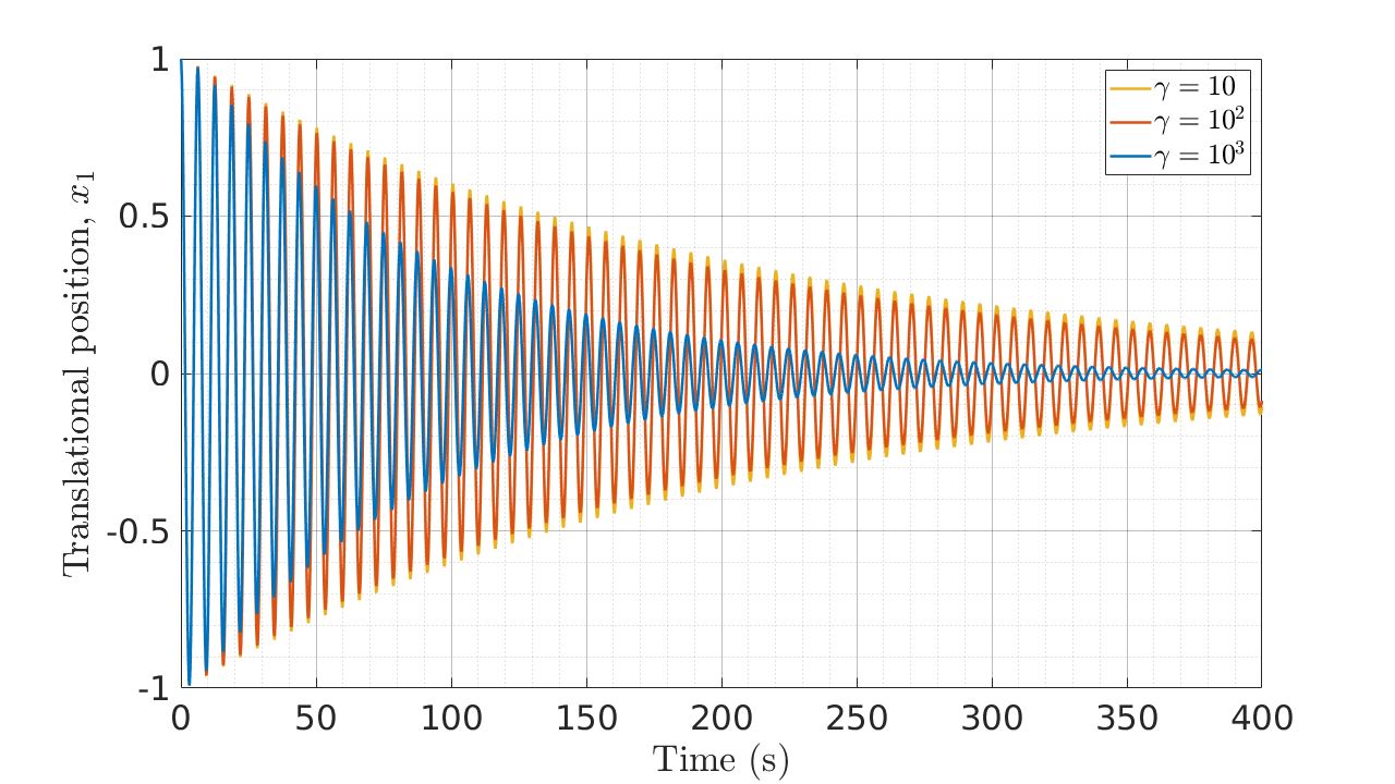
Figure 1: Evolution of the translational position of the TORA system ($\sigma=0.1$) controlled by an unstable FORE with soft resets and various values of the soft-reset parameter $\gamma$. With $\gamma=0$ the origin is not asymptotically stable. With $\gamma>0$ large enough, the origin is asymptotically stable; oscillations are smaller and the convergence is faster for larger $\gamma$.

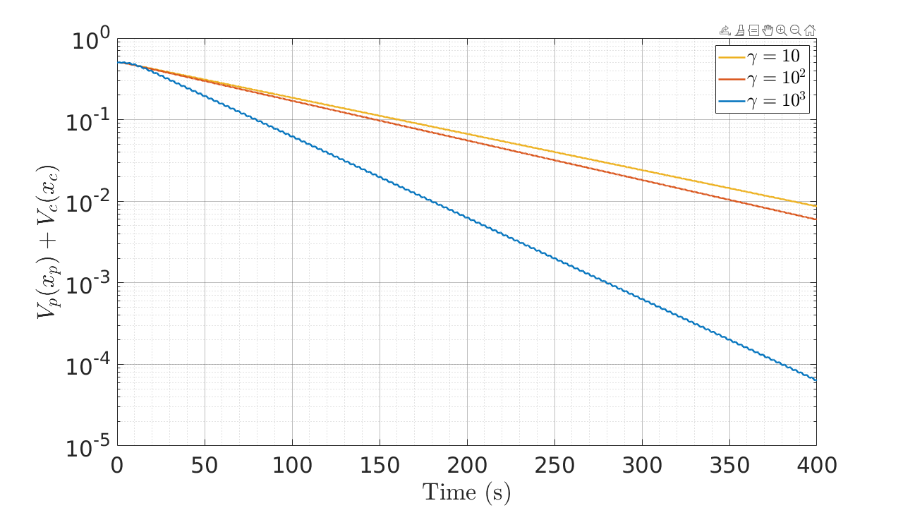
Figure 2: Evolution of the total energy for the TORA system ($\sigma=0.1$) controlled by an unstable FORE with soft resets and various values of the soft-reset parameter $\gamma$. The convergence rate increases as $\gamma$ increases.

VI-B Multi-link robotic manipulator

We consider the planar $2$-link robotic manipulator from [30, App. A.10]. The state variable is $q=(q_{1},q_{2})$, where $q_{1}$ is the angular position of the first link, measured with respect to the horizontal axis of the plane, and $q_{2}$ is the angular position of the second link, measured with respect to the line segment from the first joint to the second joint. We define the potential energy as

$$P(q) \coloneqq 784.8\sin(q_{1})+245.25\sin(q_{1}+q_{2})$$

$$\quad+\frac{\varrho}{2}\left(\left|q_{1}+\frac{\pi}{2}\right|^{2}+\left|q_{2}\right|^{2}\right),$$

where $\varrho$ is a small positive number to ensure radial unboundedness and positive definiteness of $q\mapsto P(q)-P(q^{*})$ with respect to $q^{*}\coloneqq(-\frac{\pi}{2},0)$. With $g(q)\coloneqq\partial{P}(q)/\partial{q}$ for all $q\in\mathbb{R}^{n}$, the dynamic equation of the manipulator is

$$\ddot{q}=M^{-1}(q)[u-C(q,\dot{q})\dot{q}-g(q)],$$ (62)

with $u$ being the system input, and with $M$ and $C$ given by [30, Eqs. A.36-A.38]. Defining the state $x_{p}=(q,\dot{q})$, passivity from $u$ to $\dot{q}$ can be shown using the continuously differentiable, positive definite, radially unbounded energy function

$$V_{p}(x_{p}) =\frac{1}{2}\dot{q}^{T}M(q)\dot{q}+P(q)-P(q^{*}).$$ (63)

For the system having the translated state $\tilde{x}_{p}\coloneqq(\tilde{q},\dot{q})$ with $\tilde{q}\coloneqq q-q^{*}$, global detectability does not hold because, for small $\varrho$, $g(q)$ can be zero at some points where $q\neq q^{*}$. However, $g(q)$ is uniquely zero at $q^{*}$ in the region where $q-q^{*}\in[-\pi,\pi]^{2}$. Thus, local detectability holds for trajectories $\tilde{x}_{p}$ for which $\tilde{q}(t)\in[-\pi,\pi]^{2}$ for all $t$. Figure 3 shows the trajectory of $q_{1}$ and Figure 4 shows the evolution of the energy when the system is controlled using measurements of $\dot{q}$, with the controller having input $u_{c}=-\dot{q}$ and having the form

$$f_{c}(z_{c}) =A_{c}x_{c}+B_{c}u_{c},$$ (64a)

$$g_{c}(z_{c}) =0,$$ (64b)

$$h_{c}(z_{c}) =C_{c}x_{c},$$ (64c)

with $A_{c}=-I_{n_{c}}$, $B_{c}=100I_{n_{c}}$, and $C_{c}=I_{n_{c}}$. With the chosen system matrices, the controller’s energy function is given by $V_{c}(x)=0.005|x_{c}|^{2}$. The initial condition is $(\pi/2,-\pi/4)$, which we have chosen so that, via the closed-loop stability verified by the Lyapunov function $V_{p}(x_{p})+V_{c}(x_{c})$, the trajectories satisfy $\tilde{q}(t)\in[-\pi,\pi]^{2}$ for all $t$. The soft resets are implemented with $\gamma=10^{3}$ and

$$M =\left[\begin{array}[]{cc}0&-\frac{1}{2}I_{n_{c}}\\ -\frac{1}{2}I_{n_{c}}&0\end{array}\right].$$ (67)

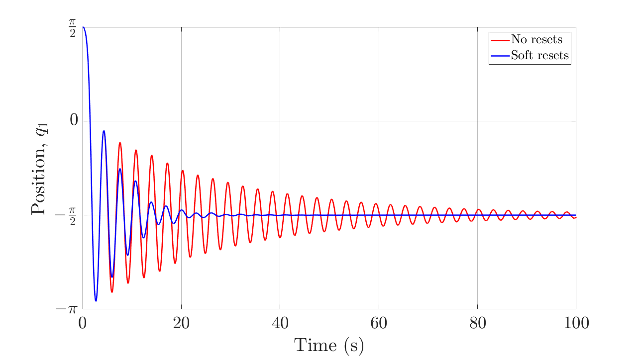
Figure 3: Angular position trajectory of the first link in a $2$-link robotic manipulator, controlled using a stable FORE with angular velocities as inputs and using soft resets.

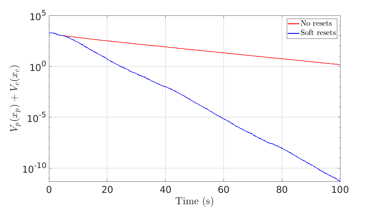
Figure 4: Evolution of the total energy of a $2$-link robotic manipulator, controlled using a stable FORE with angular velocities as inputs and using soft resets.

VI-C Strongly convex, non-quadratic accelerated optimization

We consider the strongly convex function $\phi:\mathbb{R}^{n_{p}}\to\mathbb{R}$ from [31, Eq. 17], given by

$$\phi(x) =\sum_{i=1}^{p}\hat{\phi}(a_{i}^{T}x-b_{i})+\frac{1}{2}|x|^{2},$$ (68)

$$\hat{\phi}(\alpha) =\begin{dcases}\frac{1}{2}\alpha^{2}\exp(-r/\alpha),&\alpha>0\\ 0&\alpha\leq 0,\end{dcases}$$ (69)

with $r=10^{-6}$. We randomly generate the entries of $A$ and $b$ as described in [31], such that $|A|=\sqrt{L-1}$, where $L=10^{4}$ is the Lipschitz constant of $\nabla\phi$. To apply our proposed reset control approach toward the minimization of $\phi$, we define the plant system

$$f_{p}(x_{p},u_{p}) =u_{p},$$ (70)

$$h_{p}(x_{p},u_{p}) =\nabla\phi(x_{p}),$$ (71)

and we take the control system to be defined by (64) with $n_{c}=n_{p}$, $A_{c}=-KI_{n_{c}}$, $B_{c}=I_{n_{c}}$, and $C_{c}=I_{n_{c}}$, where $K\in\mathbb{R}_{>0}$ is a tuning parameter. The top plot in Figure 5 shows the evolution of $|\nabla\phi(x_{p})|$ for the case of $n_{p}=5$, $p=10$, and $K=2$. The soft resets are implemented with $K=1$, $\gamma=30$, and $M$ given by (67). The bottom plot in Figure 5 shows the evolution of $|\nabla\phi(x_{p})|$ for the case of $n_{p}=50$, $p=5$, and $K=2$. The soft resets are implemented with $K=2$, $\gamma=20$, and $M$ given by (67).

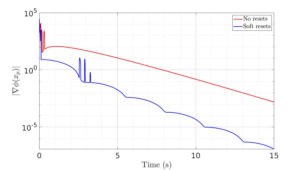
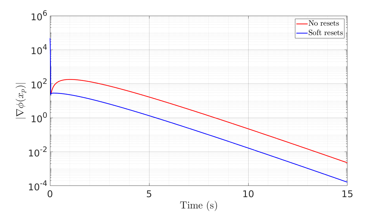
Figure 5: Performance of reset control for strongly convex optimization.

VII Conclusions

We have introduced nonlinear, passive, soft-reset control systems as an alternative to hard-reset control systems. Soft-reset control systems avoid the formalism of hybrid systems and are straightforward to implement, without any temporal regularization of other “robustifying” mechanisms. A passive hard-reset control system can be implemented as a soft-reset control system when it admits a strongly convex energy function. Asymptotic stability for the origin of the interconnection of a passive soft-reset control system with a nonlinear, passive plant has been established, under weak detectability conditions. The theory has been illustrated on two mechanical systems and also in the context of optimization of a strongly convex, non-quadratic objective function.

References

• [1] J. C. Clegg. A nonlinear integrator for servomechanisms. Transactions A.I.E.E., 77 (Part II):41–42, 1958.
• [2] K.R. Krishnan and I.M. Horowitz. Synthesis of a non-linear feedback system with significant plant-ignorance for prescribed system tolerances. International Journal of Control, 19(4):689–706, 1974.
• [3] I.M. Horowitz and P. Rosenbaum. Non-linear design for cost of feedback reduction in systems with large parameter uncertainty. International Journal of Control, 21(6):977–1001, 1975.
• [4] C.V. Hollot. Revisiting Clegg integrators: periodicity, stability and IQCs. In IFAC Proceedings, volume 30, pages 31–38, 1997.
• [5] H. Hu, Y. Zheng, Y. Chait, and C. V. Hollot. On the zero-input stability of control systems with Clegg integrators. In Proceedings of the 1997 American Control Conference, volume 1, pages 408–410, 1997.
• [6] C. V. Hollot, Y. Zheng, and Y. Chait. Stability analysis for control systems with reset integrators. In Proceedings of the 36th IEEE Conference on Decision and Control, volume 2, pages 1717–1719 vol.2, 1997.
• [7] H. Hu, Y. Zheng, C.V. Hollot, and Y. Chait. On the stability of control systems having Clegg integrators. In Topics in Control and its Applications. Springer, London, 1999.
• [8] Q. Chen, C. V. Hollot, and Y. Chait. Stability and asymptotic performance analysis of a class of reset control systems. In Proceedings of the 39th IEEE Conference on Decision and Control, pages 251–256, 2000.
• [9] Orhan Beker, C.V. Hollot, Y. Chait, and H. Han. Fundamental properties of reset control systems. Automatica, 40(6):905 – 915, 2004.
• [10] R. Goebel, R. G. Sanfelice, and A. R. Teel. Hybrid Dynamical Systems: Modeling, Stability, and Robustness. Princeton University Press, 2012.
• [11] D. Nesic, L. Zaccarian, and A.R. Teel. Stability properties of reset systems. Automatica, 44(8):2019–2026, 2008.
• [12] D. Nesic, A. R. Teel, and L. Zaccarian. Stability and performance of SISO control systems with first-order reset elements. IEEE Transactions on Automatic Control, 56(11):2567–2582, 2011.
• [13] A. Baños and A. Barreiro. Reset Control Systems. Springer, 2012.
• [14] W.H.T.M. Aangenent, G. Witvoet, W.P.M.H. Heemels, M.J.G. van de Molengraft, and M. Steinbuch. Performance analysis of reset control systems. International Journal of Robust and Nonlinear Control, 20(11):1213–1233, 2010.
• [15] C. Prieur, I. Queinnec, S. Tarbouriech, and L. Zaccarian. Analysis and synthesis of reset control systems. In Foundations and Trends in Systems and Control, volume 6 (2-3), pages 117–338. NowPublishers, 2018.
• [16] R. T. Bupp, D. S. Bernstein, V. Chellaboina, and W. M. Haddad. Resetting virtual absorbers for vibration control. J. Vibr. Control, 6:61–83, 2000.
• [17] W.M. Haddad, V. Chellaboina, Q. Hui, and S.G. Nersesov. Energy- and entropy-based stabilization for lossless dynamical systems via hybrid controllers. IEEE Trans. Autom. Control, 52(9):1604–1614, 2007.
• [18] W.M. Haddad, V. Chellaboina, and S.G. Nersesov. Impulsive and Hybrid Dynamical Systems. Princeton University Press, 2006.
• [19] K. J. Astrom and B. M. Bernhardsson. Comparison of Riemann and Lebesgue sampling for first order stochastic systems. In Proceedings of the 41st IEEE Conference on Decision and Control, pages 2011–2016, 2002.
• [20] P. Tabuada. Event-triggered real-time scheduling of stabilizing control tasks. IEEE Trans. Automat. Control, 52(9):1680–1685, 2007.
• [21] S.J.L.M. van Loon, B.G.B. Hunnekens, W.P.M.H. Heemels, N. van de Wouw, and H. Nijmeijer. Split-path nonlinear integral control for transient performance improvement. Automatica, 66:262–270, 2016.
• [22] J.H. Le and A.R. Teel. Hybrid heavy-ball systems: Reset methods for optimization with uncertainty. In 2021 American Control Conference (ACC), pages 2236–2241, 2021.
• [23] M. Baradaran, J.H. Le, and A.R. Teel. Analyzing the effect of persistent asset switches on a class of hybrid-inspired optimization algorithms. In 2021 American Control Conference (ACC), pages 3422–3427, 2021.
• [24] A.R. Teel. Continuous-time implementation of reset control systems. In Trends in Nonlinear and Adaptive Control – A tribute to Laurent Praly for his 65th birthday, Lecture Notes in Control and Information Sciences. Springer, 2021.
• [25] S. Boyd and L. Vandenberghe. Convex Optimization. Cambridge University Press, 2004.
• [26] E.P. Ryan. A universal adaptive stabilizer for a class of nonlinear systems. Systems & Control Letters, 16(3):209 – 218, 1991.
• [27] E. P. Ryan. An integral invariance principle for differential inclusions with applications in adaptive control. SIAM J. Control Optim., 36(3):960–980, 1998.
• [28] C-J. Wan, D.S. Bernstein, and V.T. Coppola. Global stabilization of the oscillating eccentric rotor. Nonlinear Dynamics, 10(1):49–62, 1996.
• [29] M. Jankovic, D. Fontaine, and P. V. Kokotovic. TORA example: cascade- and passivity-based control designs. IEEE Transactions on Control Systems Technology, 4(3):292–297, 1996.
• [30] H.K. Khalil. Nonlinear Control. Pearson Education, Inc., 2015.
• [31] B. Van Scoy, R. A. Freeman, and K. M. Lynch. The fastest known globally convergent first-order method for minimizing strongly convex functions. IEEE Control Systems Letters, 2(1):49–54, 2018.