Unsupervised Information Obfuscation for Split Inference of
Neural Networks

Abstract

Splitting network computations between the edge device and a server enables low edge-compute inference of neural networks but might expose sensitive information about the test query to the server. To address this problem, existing techniques train the model to minimize information leakage for a given set of sensitive attributes. In practice, however, the test queries might contain attributes that are not foreseen during training.

We propose instead an unsupervised obfuscation method to discard the information irrelevant to the main task. We formulate the problem via an information theoretical framework and derive an analytical solution for a given distortion to the model output. In our method, the edge device runs the model up to a split layer determined based on its computational capacity. It then obfuscates the obtained feature vector based on the first layer of the server’s model by removing the components in the null space as well as the low-energy components of the remaining signal. Our experimental results show that our method outperforms existing techniques in removing the information of the irrelevant attributes and maintaining the accuracy on the target label. We also show that our method reduces the communication cost and incurs only a small computational overhead.

1 Introduction

In recent years, the surge in cloud computing and machine learning has led to the emergence of Machine Learning as a Service (MLaaS), where the compute capacity of the cloud is used to analyze the data generated on edge devices. One shortcoming of the MLaaS framework is the leakage of the clients’ privacy-sensitive data to the cloud server. To address this problem, several cryptography-based solutions have been proposed which provide provable security at the cost of increasing the communication cost and delay of the cloud inference by orders of magnitude (Juvekar et al., 2018; Rathee et al., 2020). Such cryptography-based solutions are applicable in use-cases where delay is tolerable such as healthcare (Zhu et al., 2020), but not in scenarios where millions of clients request fast and low communication cost responses such as in Amazon Alexa or Apple Siri applications. A light-weight alternative to cryptographic solutions is to hide sensitive information on the edge device, e.g., by blurring images before sending them to the server (Vishwamitra et al., 2017). This approach, however, is task-specific and is not viable for generic applications.

Another approach is split inference which provides a generic and computationally efficient data obfuscation framework (Kang et al., 2017; Chi et al., 2018). In this approach, the service provider trains the model and splits it into two sub-models, $M_{c}$ and $M_{s}$, where $M_{c}$ contains the first few layers of the model and $M_{s}$ contains the rest. At inference time, the client runs $M_{c}$ on the edge device and sends the resulting feature vector $z=M_{c}(x)$ to the server, which then computes the target label as $\hat{y}^{\mathrm{tar}}=M_{s}(z)$. To protect the sensitive content of the client’s query, the model is required to be designed such that $z$ only contains the information related to the underlying task. This aligns well with the recent privacy laws, such as GDPR (EU, 2016), that restrict the amount of collected information to the necessary minimum. For instance, when sending facial features for cell-phone authentication, the client does not want to disclose other information such as their mood or their makeup. We denote such hidden attributes as $y^{\mathrm{hid}}$ in the remainder of this paper.

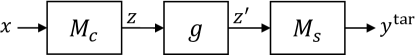
Figure 1: Unsupervised data obfuscation in split inference setting. $M_{c}$ and $M_{s}$ are the client and server models, respectively, and $g$ is the obfuscation function. The client computes $z^{\prime}=g(M_{c}(x))$ and sends $z^{\prime}$ to the server to predict the target attribute as $\hat{y}^{\mathrm{tar}}=M_{s}(z^{\prime})$. The obfuscator is designed to minimize the content in $z$ that is irrelevant to $y^{\mathrm{tar}}$, and also to be efficient enough to run on the edge device.

Current methods for data obfuscation in split inference aim to remove the information corresponding to a known list of hidden attributes. For example, adversarial training (Feutry et al., 2018) and noise injection (Mireshghallah et al., 2020) methods minimize the accuracy of an adversary model $M_{a}(z)$ on $y^{\mathrm{hid}}$, and the information bottleneck method (Osia et al., 2018) trains the model to minimize the mutual information between the query $z$ and $y^{\mathrm{hid}}$. The set of hidden attributes, however, can vary from one query to another. Hence, it is not feasible to foresee all types of attributes that could be considered sensitive for a specific MLaaS application. Moreover, the need to annotate inputs with all possible hidden attributes significantly increases the training cost as well.

In this paper, we propose an alternative solution in which, instead of removing the information that is related to a set of sensitive attributes, we discard the information that is not used by the server model to predict the target label. Our contributions are summarized in the following:

• We propose an unsupervised obfuscation mechanism, depicted in Figure 1, and formulate a general optimization problem for finding the obfuscated feature vector $z^{\prime}=g(z)$. The formulation is based on minimization of mutual information between $z$ and $z^{\prime}$, under a distortion constraint on model output $\|M_{s}(z)-M_{s}(z^{\prime})\|$. We then devise a practical solution for a relaxation of the problem using the SVD of the first layer of $M_{s}$.

• We perform extensive experiments on several datasets and show that our methods provide better tradeoffs between accuracy and obfuscation compared to existing approaches such as adversarial training, despite having no knowledge of the hidden attribute at training or inference phases. We also investigate the role of the edge computation and show that, with higher edge computation, the client obtains better obfuscation at the same target accuracy.

2 Problem Statement

Let $M_{c}$ and $M_{s}$ be the client and server models, respectively, and $g$ be the obfuscation function. We consider a split inference setup, where the model $M_{s}\circ M_{c}$ is trained with a set of examples $\{x_{i}\}_{i=1}^{N}$ and their corresponding target labels $\{y^{\mathrm{tar}}_{i}\}_{i=1}^{N}$. At inference phase, clients run $g\circ M_{c}$ on their data and send $z^{\prime}=g(z)$ to the server, where $z=M_{c}(x)$. The goal of the data obfuscation is to generate $z^{\prime}$ such that it contains minimal information about the sensitive attributes, yet the predicted target label for $z^{\prime}$ is similar to that of $z$, i.e., $M_{s}(z^{\prime})\approx M_{s}(z)$. We consider the unsupervised data obfuscation setting, where the sensitive attributes are not available at training or inference phases, i.e., the obfuscation algorithm is required to be generic and remove information about any attribute that is irrelevant to the target label.

2.1 Threat Model

Client model. Upon receiving the service, the client decides on the best tradeoff of accuracy, data obfuscation, and computational efficiency, based on their desired level of information protection and also the computational capability of the edge device. Similar mechanisms are already in use in AI-on-the-edge applications. For example, in the application of unlocking smart phones with face recognition, the client can specify the required precision in face recognition, where a lower precision will provide faster authentication at the cost of lower security (Chokkattu, 2019).

Server model. The server is assumed to be honest-but-curious. It cooperates in providing an inference mechanism with minimum information leakage to abide by law enforcement (EU, 2016) or to have competitive advantage in an open market. The server performs inference of the target attribute $y^{\mathrm{tar}}$, but might try to extract the sensitive information from the obfuscated feature vector, $z^{\prime}$, as well.

Adversary model. The adversary tries to infer sensitive attribute(s), $y^{\mathrm{hid}}$, from the obfuscated feature vector, $z^{\prime}$. We consider a strong adversary with full knowledge of the client and server models, the training data and training algorithm, and the client’s obfuscation algorithm and setting. The client and the server, however, do not know the adversary’s algorithm and are not aware of the sensitive attributes that the adversary tries to infer.

3 Related Work

Prior work has shown that representations learned by neural networks can be used to extract sensitive information (Song and Shmatikov, 2019) or even reconstruct the raw data (Mahendran and Vedaldi, 2015). Current methods for data obfuscation can be categorized as follows.

Cryptography-based Solutions. A class of public-key encryption algorithms protects the data in the transmission phase (Al-Riyami and Paterson, 2003), but cannot prevent data exposure to a curious server. Nevertheless, these methods can be used in conjunction with our approach to strengthen the defense against external adversaries. Another type of cryptographic methods allows running inference directly on the encrypted data (Rathee et al., 2020) at the cost of significant communication and computation overhead. As an example, using the state-of-the-art cryptographic method, performing inference on a single ImageNet data takes about half an hour and requires $\sim 32$GB data transmission (Rathee et al., 2020). We consider scenarios where the server provides service to millions of users (e.g., in Amazon Alexa or Apple Siri applications), and users expect low communication and fast response. Hence, classic solutions for secure function evaluation are not applicable to our scenario due to their high computational and communication cost.

Noise Injection. In this method, the client sends a noisy feature $z^{\prime}\sim h_{\theta}(z)$ instead of $z$ to the server, where $z^{\prime}$ is drawn from a randomized mechanism $h_{\theta}(\cdot)$ parameterized by $\theta$ (e.g., a Gaussian distribution). A typical approach one could employ is differential privacy (DP) (Dwork, 2006; Dwork et al., 2006, 2014), which guarantees that the distribution of $z^{\prime}$ does not differ too much for any two inputs $z_{1}$ and $z_{2}$. Using DP, however, can lead to a large loss of accuracy  (Kasiviswanathan et al., 2011; Ullman, 2018; Kairouz et al., 2019). To maintain the utility of the model, (Mireshghallah et al., 2020) proposed to solve the following:

$$\small\underset{\theta}{\min}\ \ \mathcal{L}(M_{s}(z^{\prime}),y^{\mathrm{tar}})-\gamma\mathcal{L}(M_{a}(z^{\prime}),y^{\mathrm{hid}})-\alpha|z^{\prime}-z|,$$ (1)

where the first and second terms denote the cross entropy loss for the server and adversary, respectively. In general, while noise addition improves the privacy, it has been shown to significantly reduce the accuracy (Liu et al., 2019; Li et al., 2019).

Information Bottleneck (IB) is proposed to obfuscate the information related to a known set of sensitive attributes, $y^{\mathrm{hid}}$. Let $I(\cdot,\cdot)$ denote mutual information. The idea is to train $M_{c}$ that maximizes $I(z,y^{\mathrm{tar}})$ while minimizing $I(z,y^{\mathrm{hid}})$ (Osia et al., 2018; Moyer et al., 2018). The optimization is formulated as follows:

$$\underset{M_{c}}{\max}\quad I(M_{c}(x),y^{\mathrm{tar}})-\gamma I(M_{c}(x),y^{\mathrm{hid}})-\beta I(M_{c}(x),x).$$ (2)

Adversarial Training (AT) is an effective method for obfuscating the information of a known set of sensitive attributes, while maintaining the accuracy on the target label. AT solves the following min-max optimization problem:

$$\underset{M_{c},M_{s}}{\max}\ \underset{M_{a}}{\min}\ \underset{x,y^{\mathrm{tar}},y^{\mathrm{hid}}}{\mathbb{E}}[\gamma\mathcal{L}(y^{\mathrm{hid}},M_{a}\circ M_{c}(x))-\mathcal{L}(y^{\mathrm{tar}},M_{s}\circ M_{c}(x))],$$ (3)

where $\mathcal{L}$ denotes the cross-entropy loss. The above objective can be achieved through an adversarial training method (Edwards and Storkey, 2016; Hamm, 2017; Xie et al., 2017; Li et al., 2018; Feutry et al., 2018; Li et al., 2019; Huang et al., 2017). Upon convergence, the model $M_{c}$ generates $z$, using which $M_{a}$ cannot accurately estimate $y^{\mathrm{hid}}$, yet $M_{s}$ accurately predicts $y^{\mathrm{tar}}$.

Existing obfuscation methods for split inference have several limitations. Except differential privacy which often significantly reduces the accuracy on $y^{\mathrm{tar}}$, the underlying assumption in the above methods is that a set of hidden attributes $y^{\mathrm{hid}}$ is provided at training time. In practice, however, it might not be feasible to foresee and identify all possible sensitive attributes and annotate the training data accordingly. It also contradicts deployment at-scale since whenever a new attribute needs to be protected, the client model has to be retrained and re-distributed to all edge devices that use the service. Current approaches also often provide a poor tradeoff between accuracy and preventing the information leakage. Moreover, the tradeoff of accuracy and obfuscation with the client-side computation is not well studied in the split learning framework. In this paper, we characterize this tradeoff and propose to remove the content irrelevant to the main task, instead of obfuscating a predefined set of sensitive attributes. We empirically show that our method reduces the attack accuracy on hidden attributes, which are not known to the client or the server at training or inference times, at a small or no cost to the accuracy on the target label.

4 The Proposed Method

4.1 Problem Formulation

Let $z\in\mathbb{R}^{n\times 1}$ be the feature vector and $y^{\mathrm{tar}}$ be the corresponding label. Our goal is to design the obfuscation function, $g$, such that $z^{\prime}=g(z)$ contains the necessary and sufficient information about $y^{\mathrm{tar}}$. Specifically, we want to (i) minimize the information that $z^{\prime}$ carries about $z$, while (ii) maintaining the utility of the model for predicting $y^{\mathrm{tar}}$ as much as possible. We formulate the problem as follows:

$$\underset{z^{\prime}}{\min\ }I(z^{\prime},z)\quad\mbox{ s.t. }\|M_{s}(z^{\prime})-M_{s}(z)\|\leq\epsilon.$$ (4)

The objective function in (4) minimizes the mutual information of $z^{\prime}$ and $z$, while bounding the distortion to the model output. Note that our formulation is different from the information bottleneck (1) proposed by (Osia et al., 2018; Moyer et al., 2018) in that it does not use $y^{\mathrm{hid}}$ and, hence, is unsupervised with respect to hidden attributes.

Let $H(\cdot)$ denote the entropy function. We have:

$$I(z^{\prime},z)=H(z^{\prime})-H(z^{\prime}|z)=H(z^{\prime}),$$

where the second equality holds since the obfuscation function $g$ is a deterministic algorithm and thus $H(z^{\prime}|z)=0$. The objective in (4) can therefore be written as:

$$\underset{z^{\prime}}{\min\ }H(z^{\prime})\quad\mbox{ s.t. }\|M_{s}(z^{\prime})-M_{s}(z)\|\leq\epsilon.$$ (5)

Intuitively, a small $H(z^{\prime})$ indicates that, from the server’s point of view, the incoming queries look similar. For example, in face recognition applications, only basic properties of face images are transmitted to the server and other irrelevant attributes that would make the images different in each query, such as the background or makeup, are obfuscated.

4.2 Obfuscation for Linear Layers

Our goal is to develop a low-complexity obfuscation function, $g$, that solves (5) with respect to the server’s model, $M_{s}$. Figure 1 shows the block diagram of the method. In its general form, the function $g$ can be viewed as an auto-encoder (AE) network that is trained with the objective of (5). Such a network would be, however, computationally complex to run on edge devices and defeats the purpose of sending activations to the server for low-complexity inference.

To address the computational complexity problem, we design the obfuscation function with respect to the first linear layer (a convolutional or fully-connected layer) of $M_{s}$. For linear models, the objective in (5) can be written as:

$$\underset{z^{\prime}}{\min\ }H(z^{\prime})\quad\mbox{ s.t. }\|Wz-Wz^{\prime}\|\leq\epsilon,$$ (6)

where $W\in\mathbb{R}^{m\times n}$ is the weight matrix. In the following, we present our analysis for the linear models.

Definition 1.

Let $W_{m\times n}=U_{m\times m}S_{m\times n}V_{n\times n}^{T}$ denote the singular value decomposition (SVD) of $W$. The columns of $V^{T}$ provide an orthonormal basis $\{v_{k}\}_{k=1}^{n}$. We write:

$$z=\sum_{k=1}^{n}\alpha_{k}v_{k}=\sum_{k=1}^{n}z_{k},\quad\alpha_{k}=v_{k}^{T}\cdot z.$$ (7)

We have the following Lemmas.

Lemma 1.

If $z\sim N(\mathbf{0},\sigma^{2}\mathbf{I})$, then $\alpha_{k}$’s are independent random variables with $\alpha_{k}\sim N(0,\sigma^{2})$.

Proof.

Since $\alpha_{k}=v_{k}^{T}\cdot z$, it is Gaussian with the following mean and variance:

$$\mathbb{E}[\alpha_{k}]=v_{k}^{T}\cdot\mathbb{E}[z]=0,\qquad\mathbb{E}[\alpha^{2}_{k}]=v_{k}^{T}\cdot\mathbb{E}[zz^{T}]\cdot v_{k}=\sigma^{2}v_{k}^{T}\cdot v_{k}=\sigma^{2}.$$

Assume $i\neq j$. We have:

$$cov(\alpha_{i},\alpha_{j})=\mathbb{E}[\alpha_{i}\cdot\alpha_{j}]-\mathbb{E}[\alpha_{i}]\cdot\mathbb{E}[\alpha_{j}]=v_{i}^{T}\cdot\mathbb{E}[zz^{T}]\cdot v_{j}=0.$$

Also, $\beta=c_{1}\alpha_{i}+c_{2}\alpha_{j}=(c_{1}v_{i}^{T}+c_{2}v_{j}^{T})\cdot z=v^{\prime T}z$. Therefore, since $cov(\alpha_{i},\alpha_{j})=0$ and $\beta$ is Gaussian for any $c_{1}$ and $c_{2}$, $\alpha_{k}$’s are independent random variables. ∎

Lemma 2.

For $z\sim N(\mathbf{0},\sigma^{2}\mathbf{I})$, we have $H(z_{i}|z_{j})=H(z_{i}),\forall i\neq j$.

Proof.

Assume $i\neq j$. We have:

$$cov(z_{i},z_{j}) =\mathbb{E}[z_{i}\cdot z_{j}^{T}]-\mathbb{E}[z_{i}]\cdot\mathbb{E}[z_{j}]^{T}=\mathbb{E}[\alpha_{i}\alpha_{j}]v_{i}\cdot v_{j}^{T}-\mathbb{E}[\alpha_{i}]\mathbb{E}[\alpha_{j}]v_{i}\cdot v_{j}^{T}=\mathbf{0}.$$

Also, $x=c_{1}z_{i}+c_{2}z_{j}=c_{1}\alpha_{i}v_{i}+c_{2}\alpha_{j}v_{j}$. According to Lemma 1, $\alpha_{k}$’s are independent Gaussian random variables. Thus, $x$ is multivariate Gaussian for any $c_{1}$ and $c_{2}$. Hence, $z_{k}$’s are independent random vectors and $H(z_{i}|z_{j})=H(z_{i}),\forall i\neq j$. ∎

Lemma 3.

For $z\sim N(\mathbf{0},\sigma^{2}\mathbf{I})$, we have $H(z)=\sum_{k=1}^{n}H(\alpha_{k})$.

Proof.

Since $z_{k}=\alpha_{k}v_{k}=(v_{k}^{T}z)v_{k}$, we have $H(z_{k}|z)=0$. Lemma 2 also shows $H(z_{i}|z_{j})=H(z_{i}),\forall i\neq j$. Hence:

$$H(z,z_{1},\dots,z_{n})=H(z)+\sum\limits_{k=1}^{n}H(z_{k}|z,z_{1},\dots,z_{k-1})=H(z).$$

The left hand side can be also written as:

$$H(z,z_{1},\dots,z_{n}) =H(z_{1})+H(z|z_{1})+\sum\limits_{k=2}^{n}H(z_{k}|z,z_{1},\dots,z_{k-1})$$

$$=H(z_{1})+H(z|z_{1})$$

$$=H(z_{1})+H(z_{2},\dots,z_{n})$$

$$=H(z_{1})+\sum\limits_{k=2}^{n}H(z_{k}|z_{2},\dots,z_{k-1})$$

$$=\sum\limits_{k=1}^{n}H(z_{k}).$$

Hence, $H(z)=\sum\limits_{k=1}^{n}H(z_{k})$. We also have:

$$\begin{array}[]{lll}H(z_{k},\alpha_{k})&=H(z_{k})+H(\alpha_{k}|z_{k})&=H(z_{k})\\ &=H(\alpha_{k})+H(z_{k}|\alpha_{k})&=H(\alpha_{k}).\end{array}$$

Therefore, $H(z_{k})=H(\alpha_{k})$, and $H(z)=\sum\limits_{k=1}^{n}H(\alpha_{k})$. ∎

Lemma 4.

Let $z=\sum_{k=1}^{n}\alpha_{k}v_{k}$ and $z^{\prime}=\sum_{k=1}^{n}\alpha^{\prime}_{k}v_{k}$. We have $\|W(z-z^{\prime})\|=\sqrt{\sum_{k=1}^{m}(\alpha_{k}-\alpha^{\prime}_{k})^{2}s_{k}^{2}}$, where $s_{k}$ is the $k$-th singular value of $W$.

Proof.

We have:

$$\ W(z-z^{\prime})=USV(z-z^{\prime}) =\sum\limits_{k=1}^{n}USV((\alpha_{k}-\alpha_{k}^{\prime})v_{k})$$

$$=\sum\limits_{k=1}^{n}US((\alpha_{k}-\alpha_{k}^{\prime})\delta_{k})$$

$$=\sum\limits_{k=1}^{n}U(s_{k}(\alpha_{k}-\alpha_{k}^{\prime})\delta_{k})$$

$$=\sum\limits_{k=1}^{n}s_{k}(\alpha_{k}-\alpha_{k}^{\prime})U_{k},$$

where $\delta_{k}$ is a one-hot vector with its $k$-th element set to 1 and $U_{k}$ is the $k$-th column of $U$. Since $U_{k}$’s are orthonormal, we have $\|W(z-z^{\prime})\|=\sqrt{\sum_{k=1}^{m}(\alpha_{k}-\alpha^{\prime}_{k})^{2}s_{k}^{2}}$. ∎

The following theorem provides the solution of the objective in (6).

Theorem 1.

Let $W=USV^{T}$ as defined in Definition 1. Let $z=\sum_{k=1}^{n}\alpha_{k}v_{k}$ where $z\sim N(\mathbf{0},\sigma^{2}\mathbf{I})$ and $\alpha_{k}$’s are sorted based on the singular values of $W$. The objective in (6) is minimized by $z^{\prime}=\sum_{k=1}^{m}\alpha^{\prime}_{k}v_{k}$ where

$$\alpha^{\prime}_{k}=\begin{cases}\alpha_{k}&k<m^{\prime}\\ \alpha_{k}-\gamma\operatorname{sign}(\alpha_{k})&k=m^{\prime}\\ 0&k>m^{\prime}\end{cases},$$ (8)

where $m^{\prime}=\underset{k}{\operatorname*{argmin}}\ \epsilon_{k}\leq\epsilon$, $\epsilon_{k}=\sqrt{\sum_{i=k+1}^{m}\alpha_{i}^{2}s_{i}^{2}}$ and $\gamma=\frac{\sqrt{\epsilon^{2}-\epsilon_{m^{\prime}}^{2}}}{s_{m^{\prime}}}$.

Proof.

Using Lemmas 1 and 3, we have $H(z)=\sum_{k=1}^{n}H(\alpha_{k})$, where $\alpha_{k}\sim N(0,\sigma^{2})$. We have $H(\alpha_{k})=\frac{1}{2}\ln(2\pi e\sigma^{2})$ which is monotonically increasing in $var(\alpha_{k})=\sigma^{2}$. Hence, $H(\alpha_{k})$ can be reduced by suppressing the variance of $\alpha_{k}$, i.e., making $\alpha_{k}$’s closer to zero.

Given a distortion budget, $\epsilon$, the question now is which $\alpha_{k}$ should be modified and by how much. From the entropy perspective, based on the assumptions above and Lemma 3, reducing the variance of each $\alpha_{k}$ reduces the entropy by the same amount for all $k$. Lemma 4, however, states that modifying $\alpha_{k}$ by $\gamma$ causes a distortion of $|\gamma|s_{k}$, where $s_{k}$ is the $k$-th singular value of $W$. Since smaller $s_{k}$’s cause smaller distortion, the solution is achieved by sorting the singular values and then modifying the $\alpha_{k}$’s corresponding to the smaller singular values towards zero one at a time until the budget $\epsilon$ is exhausted.

The following provides the solution more specifically. If $m<n$ in the weight matrix, the last $n-m$ coefficients do not contribute to $W\cdot z$ and thus can be set to zero without causing any distortion. Now, assume the coefficients in range of $m^{\prime}+1$ to $m$ are to be set to zero. The total distortion will be $\epsilon_{m^{\prime}}=\sqrt{\sum_{i=m^{\prime}+1}^{m}s_{i}^{2}\alpha_{i}^{2}}$. Also, the distortion caused by modifying $\alpha_{m^{\prime}}$ by $\gamma$ is $s_{m^{\prime}}|\gamma|$, which we will set to be equal to the remaining distortion, $\sqrt{\epsilon^{2}-\epsilon_{m^{\prime}}^{2}}$, i.e., $\gamma=\frac{\sqrt{\epsilon^{2}-\epsilon_{m^{\prime}}^{2}}}{s_{m^{\prime}}}$. This completes the proof. ∎

Definition 2.

The signal content of $z$ with respect to a matrix $W$, or simply the signal content of $z$, is the solution to (6) with $\epsilon=0$. It is denoted by $z_{\mathcal{S}}$ and defined as follows:

$$z_{\mathcal{S}}=\sum\limits_{k=1}^{m}\alpha_{k}v_{k}.$$ (9)

The remaining $n-m$ components of $z$ are called the null content defined as follows:

$$z_{\mathcal{N}}=z-z_{\mathcal{S}}=\sum_{k=m+1}^{n}\alpha_{k}v_{k}.$$ (10)

The signal content is the information that is kept after multiplying $z$ by $W$, and the null content is the discarded information. By setting $z^{\prime}=z_{\mathcal{S}}$, the client reduces the entropy without introducing any distortion to the output of $M_{s}$. We call this method distortion-free obfuscation herein. The entropy can be further reduced by removing components from the signal content as well, for which the optimal way for a desired distortion $\epsilon$ is determined by Theorem 1. We call this method distortion-bounded obfuscation in the remainder of the paper.

4.3 The Proposed Obfuscation Method

In the following, we present our framework for unsupervised data obfuscation in the split inference setup.

Training. The server trains the model $M_{s}\circ M_{c}$ with inputs $\{x_{i}\}_{i=1}^{N}$ and target labels $\{y^{\mathrm{tar}}_{i}\}_{i=1}^{N}$, where, at each epoch, various fractions of the signal content of different layers are removed (one layer at a time), so that the model becomes robust to removing the components of the signal content. The model is also trained to generate feature vectors, $z$, with uncorrelated Gaussian activations as specified in Theorem 1. To learn models with decorrelated activations, we used the penalty term proposed in (Cogswell et al., 2015) as $L_{deCov}=\frac{1}{2}(\|C\|_{F}^{2}-\|\operatorname{diag}(C)\|_{2}^{2})$, where $C$ is the covariances between activation pairs, $\|\cdot\|_{F}$ is the Frobenius norm, and the $\operatorname{diag}(\cdot)$ operator extracts the main diagonal of a matrix into a vector. Additionally, the distribution of $z$ is forced to be close to Gaussian using the VAE approach (Kingma and Welling, 2013), i.e., by learning to generate $z$ from a variational distribution with a Gaussian prior.

Inference. Upon providing the service, the server also provides a profile of the average reduction in target accuracy by removing a given fraction of the signal content for each split layer. The client first decides on the number of layers to be run locally on the edge device (determined based on the compute capacity) and then on the fraction of the signal content to maintain (determined based on the desired accuracy). For inference, the client computes the obfuscated feature vector $z^{\prime}=g(M_{c}(x))$ and sends it to the server. The server then performs the rest of the computation and obtains $\hat{y}^{\mathrm{tar}}=M_{s}(z^{\prime})$.

Our framework provides a tradeoff between accuracy, obfuscation, and computational efficiency. Specifically, by running more layers locally (more edge computation), the client can achieve a better accuracy-obfuscation tradeoff, i.e., the same obfuscation can be obtained by discarding a smaller fraction of the signal content. Moreover, for a given split layer, the client can adjust the fraction of the signal content to be removed in order to obtain a desired tradeoff between accuracy and obfuscation. In Section 5, we provide empirical validations for the aforesaid tradeoffs.

Computational and Communication cost. Performing obfuscation requires the client to compute $m^{\prime}$ coefficients $\{\alpha^{\prime}_{k}\}_{k=1}^{m^{\prime}}$ on the edge device, where the overhead of computing each $\alpha^{\prime}_{k}$ is equivalent to $\frac{1}{m}$-th of total computation in the first layer of $M_{s}$. Therefore, the client performs an extra computation equivalent to $\frac{m^{\prime}}{m}\times$ the first layer of $M_{s}$, where $m^{\prime}\ll m$ in practice. Note that the client is not required to recover $z^{\prime}=\sum_{k=1}^{m^{\prime}}\alpha^{\prime}_{k}v_{k}$, and can send only $\{\alpha^{\prime}_{k}\}_{k=1}^{m^{\prime}}$ to the server, who has the $\{v_{k}\}$ basis and can compute $z^{\prime}$ accordingly. Therefore, our obfuscation method reduces the communication cost by a factor of $\frac{m^{\prime}}{n}$ compared to the case that the raw feature vector $z$ is sent to the server.

5 Experimental Results

5.1 Experiment Setup

Model architecture and training settings. We present the experimental results on an architecture used in prior work (Song and Shmatikov, 2019), shown in Table 1. The adversary model $M_{a}$ has the same architecture as the server model $M_{s}$. We train the models for $50$ epochs using Adam optimizer with an initial learning rate of $0.001$, which we drop by a factor of $10$ after $20$ and $40$ epochs.

Datasets. We perform our experiments on four visual datasets described below. Table 2 lists the target and hidden attributes of the datasets used.

• EMNIST (Cohen et al., 2017) is an extended version of the MNIST dataset where the labels are augmented with writer IDs. We select $13000$ samples from EMNIST written by $100$ writers with $130$ examples per writer. We then split this dataset into $10000$, $1500$, and $1500$ for training, validation, and testing. We use the digit and writer ID as the target and the hidden attributes, respectively.

• FaceScrub (Ng and Winkler, 2014; FaceScrub, 2020) is a dataset of celebrity faces labeled with gender and identity. We use gender as the target and identity as the hidden attribute. In experiments, we crop images using the face region bounding boxes specified in the annotations and resize them to $50\times 50$.

• UTKFace (Zhang et al., 2017) is a dataset of face images labeled with gender and race, which we treat as the target and the hidden attributes, respectively. The face region bounding boxes are cropped and resized to $50\times 50$.

• CelebA (Liu et al., 2015) is a dataset of celebrity images. Each image is labeled with 40 binary attributes, out of which, we select Smiling as the target attribute and {Male, Heavy_Makeup, High_Cheekbones, Mouth_Slightly_Open, Wearing_Lipstick, Attractive} as hidden attributes. These attributes have near balanced distribution of positive and negative examples. In experiments, we crop images to the face region and resize them to $73\times 60$.

Table 1: Network Architecture. Each row shows a split layer, i.e., for the split layer $i$, the input of that layer is sent to the server.

Layer	Architecture
1	CONV($3,16$), ReLU, Maxpool($2\times 2$), Batchnorm
2	CONV($3,32$), ReLU, Maxpool($2\times 2$), Batchnorm
3	CONV($3,64$), ReLU, Maxpool($2\times 2$), Batchnorm
4	FC(128), ReLU, Batchnorm
5	FC(64), ReLU, Batchnorm
6	FC($n_{\mbox{\tiny classes}}$), Softmax

Table 2: Target and hidden attributes of the datasets used.

Dataset	Target Attribute ($y^{\mathrm{tar}}$)		Hidden Attribute ($y^{\mathrm{hid}}$)
	Attribute	No. Classes	Attribute	No. Classes
EMNIST	digit	10	writer ID	100
UTKFace	gender	2	race	5
FaceScrub	gender	2	identity	530
CelebA	smiling	2	gender	2
		2	makeup	2
		2	cheekbones	2
		2	mouth-open	2
		2	lipstick	2
		2	attractive	2

Measuring obfuscation. Several methods have been proposed to measure the information leakage of intermediate feature vectors in neural networks. One approach is computing the mutual information between the query $x$ and the feature vector $z^{\prime}$ (Kraskov et al., 2004). In practice, measuring the mutual information is not tractable for high-dimensional random variables, unless certain assumptions are made about the probability distribution of the random variables of interest. A more practical approach computes the reconstruction error, $\|\widetilde{x}-x\|$, where $\widetilde{x}$ is estimated using the feature vector (Mahendran and Vedaldi, 2015). Finally, attribute leakage can be defined based on the accuracy of an adversary model that predicts the hidden label from intermediate features.

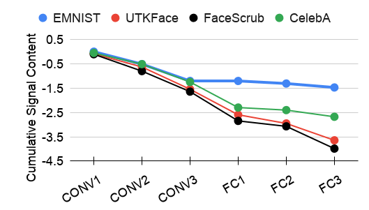
Figure 2: Cumulative preserved signal content at different layers of $M_{s}\circ M_{c}$. The model acts as an obfuscator, gradually removing the content irrelevant to the target label from one layer to the next.

In this paper, we follow the approach of predicting hidden attributes using an adversary model. Assume that each example $\{x_{i}\}_{i=1}^{N}$ has a target label $\{y^{\mathrm{tar}}_{i}\}_{i=1}^{N}$ and a hidden label $\{y^{\mathrm{hid}}_{i}\}_{i=1}^{N}$. The adversary trains the model $M_{a}$ with $(z^{\prime}_{i},y_{i}^{\mathrm{hid}})$, where $z^{\prime}_{i}=g(M_{c}(x_{i}))$ is the same feature vector that the server also receives to do inference of the target label. Note that the training of $M_{a}$ is used as a post hoc process to evaluate the leakage of sensitive attributes and does not influence the client or server’s processing. We refer to the accuracy of $M_{s}\circ g\circ M_{c}$ on $y^{\mathrm{tar}}$ as target accuracy and the accuracy of $M_{a}\circ g\circ M_{c}$ on $y^{\mathrm{hid}}$ as attack accuracy.

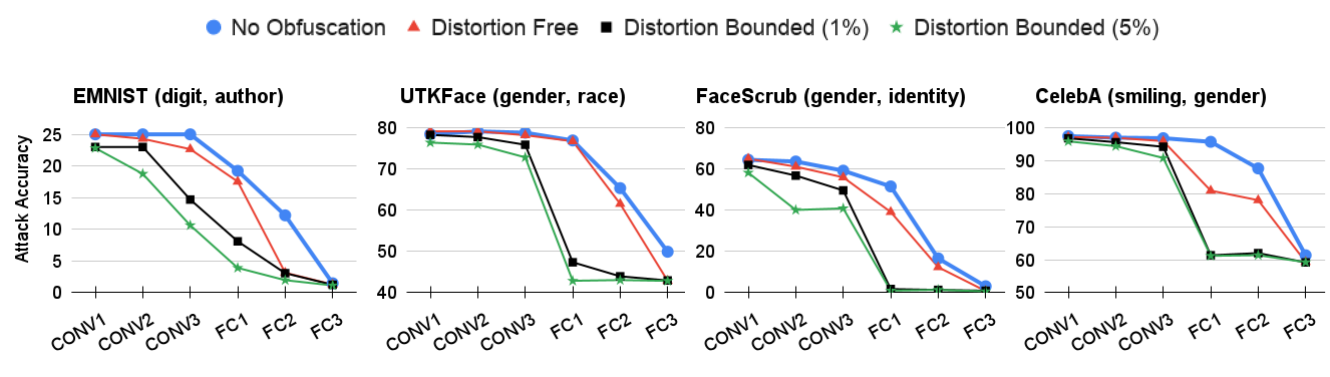
Figure 3: Attack accuracy versus the split layer for each dataset. The target/attack attributes are mentioned in the title of each sub-figure. Each colored curve corresponds to a different obfuscation method. The horizontal and vertical axes represent split layer and attack accuracy, respectively. It is desired to have a lower attack accuracy at earlier layers. The blue curves show the attack accuracy without obfuscation; the red curve represents our distortion-free obfuscation (with no loss of target accuracy); The black and green curves correspond to $1\%$ and $5\%$ of reduction in target accuracy, respectively. We observe two trends: (1) by performing more computation on the edge device (e.g., splitting at FC1 layer instead of CONV1 layer), one can achieve a lower attack accuracy. (2) for a certain split layer, our distortion free obfuscation reduces the attack accuracy of the baseline without reducing target accuracy. Our distortion-bounded accuracy provides a tradeoff between target accuracy and target accuracy. In this figure, for instance, we can see that the attack accuracy of the green curve ($5\%$ distortion) is lower than the black curve ($1\%$ distortion).

5.2 Evaluations

Cumulative signal content. We start our analysis by computing the norm of the null and signal contents in every layer of $M=M_{s}\circ M_{c}$. At each layer, the null content $z_{\mathcal{N}}$ is discarded and the signal content $z_{\mathcal{S}}$ is passed through the next layer. We compute the normalized amount of the information passed from the $i$-th layer to the next as $C_{\mathcal{S}}(z^{(i)})=\log(\frac{\|z_{\mathcal{S}}^{(i)}\|_{2}^{2}}{\|z^{(i)}\|_{2}^{2}})$, where $z^{(i)}$ and $z_{\mathcal{S}}^{(i)}$ are the activation vector and its signal content at the $i$-th layer, respectively. Figure 2 shows the cumulative amount of the signal content preserved up to the $i$-th layer, computed as $\sum_{j=1}^{i}C_{\mathcal{S}}(z^{(j)})$. The plot suggests that the model gradually removes the content irrelevant to the target label from one layer to the next, thus acting as an obfuscator.

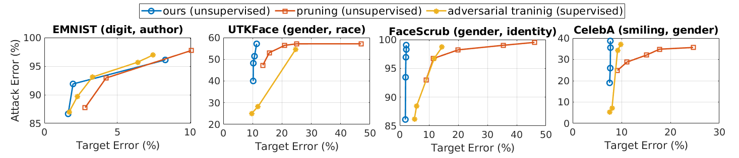
Figure 4: Comparison between our method, feature pruning, and adversarial training when splitting the model at the input of the FC1 layer. The target/attack attributes are mentioned in the title of each sub-figure. The horizontal and vertical axes show the classification error on $y^{\mathrm{tar}}$ and $y^{\mathrm{hid}}$, respectively. To extract the points of the blue curve, we obfuscate the features at the split layer with different distortion rates. For pruning, the curves are obtained by pruning the features at the split layer with different pruning ratios. For adversarial training, each point on the curve represents an adversarially trained network with different $\gamma$ parameter. Our goal is to have low error on $y^{\mathrm{tar}}$ and high error on $y^{\mathrm{hid}}$, hence, points to the upper left corner of the figures are desirable. In most cases, our method outperforms both adversarial training and pruning.

Investigating tradeoffs. Figure 3 shows the attack accuracy versus the split layer for four settings: (1) without obfuscation, (2) with distortion-free obfuscation (i.e., when $m^{\prime}=m$), and (3),(4) with distortion-bounded obfuscation such that the drop in target accuracy is at most $1\%$ and $5\%$, respectively. The results illustrate the tradeoffs between edge computation, obfuscation, and target accuracy, described in the following.

• In all four cases, the attack accuracy decreases as the network is split at deeper layers. This observation indicates that more edge computation results in lower attack accuracy at the same target accuracy.

• For each split layer, the attack accuracy of distortion-free obfuscation is less than that of the baseline (no obfuscation). This observation shows that even without decreasing the target accuracy, the feature vector can be modified to obtain a better obfuscation.

• For each split layer, the distortion-bounded obfuscation further reduces the attack accuracy at the cost of a small reduction in target accuracy. In the example analysis of Figure 3, we include the attack accuracy when the target accuracy is dropped by $1\%$ and $5\%$. As seen, by losing more target accuracy, the attack accuracy can be further reduced. The tradeoff between attack and target accuracy is controlled by the the number of preserved features, $m^{\prime}$.

Comparison to prior work. We compare our obfuscation method to two general categories of prior work:

• Supervised Obfuscation. Among existing supervised obfuscation methods introduced in Section 3, adversarial training generally provides the best tradeoff between accuracy and obfuscation. Therefore, we use adversarial training as a natural comparison baseline. We implemented the adversarial training framework proposed by (Feutry et al., 2018) and trained the models in multiple settings with different $\gamma$ parameters (Eq. 3) in range of $[0.1,1]$ to achieve the best performance.

• Unsupervised Obfuscation. Similar to our approach, pruning network weights eliminates features that do not contribute to the classification done by $M_{s}$. Since pruning does not require access to the sensitive labels, it is a natural unsupervised obfuscation baseline. We adopt the pruning algorithm proposed by (Li et al., 2016) which works based on the $L_{1}$ norm of the columns of the following layer’s weight matrix. After pruning, we fine-tune $M_{s}$ to improve its accuracy.

Figure 4 compares the tradeoffs achieved by our method with those achieved by (supervised) adversarial training and (unsupervised) pruning. In this example study, we split the network at the middle layer, i.e., the input of the $FC1$ layer. Since adversarial training specifically trains the model to obfuscate the sensitive attribute, it achieves a better tradeoff than the unsupervised pruning method. Although our method is unsupervised too, it outperforms the supervised adversarial training in most cases. The superior performance of our method is rooted in minimizing the distortion to the target accuracy while maximizing the obfuscated “unrelated” information.

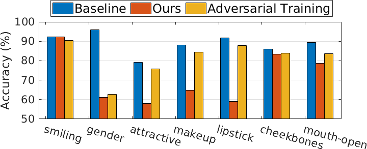
Figure 5: Accuracy on the target (Smiling) and hidden attributes. Our method obfuscates the feature vector without the knowledge of hidden attributes at training or inference times. Adversarial training (AT) method maximizes the accuracy on Smiling, while minimizing the accuracy on Gender. As seen, AT successfully reduces accuracy on Gender attribute but, unlike our method, fails to obfuscate information of other attributes. This highlights the applicability of our method in practical settings as a generic obfuscator compared to specialized techniques such as AT.

Experiment with multiple private attributes. To highlight the independence of our method from private attributes, we also do the experiments with multiple (unseen) hidden labels. Specifically, we consider the CelebA model trained to detect Smiling and evaluate two methods, (1) our method: we keep only $m^{\prime}=1$ component from the signal content of feature vector and then train one separate adversary model per hidden attribute, and (2) adversarial training: we first adversarially train an $M_{c}$ model to obfuscate Gender, and then train one separate adversary model to predict each hidden attribute.

For both of the above methods, the network is split at the input of the $FC1$ layer. As shown in Figure 5, our method outperforms adversarial training in both the target and attack accuracy. Specifically, our method results in a significantly lower attack accuracy on all hidden attributes compared to the baseline attack accuracy. The only exceptions are High_Cheekbones and Mouth_Open attributes, which highly correlate with the target attribute (a smiling person is likely to have high cheekbones and open mouth). The correlation between target and hidden attributes causes the signal content of the server and adversary models to have large overlaps and, hence, results in high attack accuracy. Also, as seen, the adversarially trained model successfully hides the information that it has been trained to obfuscate (Gender). The model, however, fails to remove information of other attributes such as Makeup or Lipstick. The results highlight the importance of the generic unsupervised obfuscation in scenarios where the sensitive attributes are not known. In such cases, unlike supervised obfuscation methods, our method successfully reduces the information leakage.

6 Conclusion

We proposed an obfuscation method for split edge-server inference of neural networks. We formulated the problem as an optimization problem based on minimizing the mutual information between the obfuscated and original features, under a distortion constraint on the model output. We derived an analytic solution for the class of linear operations on feature vectors. The obfuscation method is unsupervised with respect to sensitive attributes, i.e., it does not require the knowledge of sensitive attributes at training or inference phases. By measuring the information leakage using an adversary model, we empirically supported the effectiveness of our method when applied to models trained on various datasets. We also showed that our method outperforms existing techniques by achieving better tradeoffs between accuracy and obfuscation.

References

- Al-Riyami and Paterson (2003) Sattam S Al-Riyami and Kenneth G Paterson. Certificateless public key cryptography. In International conference on the theory and application of cryptology and information security, 2003.
- Chi et al. (2018) Jianfeng Chi, Emmanuel Owusu, Xuwang Yin, Tong Yu, William Chan, Patrick Tague, and Yuan Tian. Privacy partitioning: Protecting user data during the deep learning inference phase. arXiv preprint arXiv:1812.02863, 2018.
- Chokkattu (2019) Julian Chokkattu. How to make face unlock more secure in the Samsung Galaxy S10 line, 2019. https://www.digitaltrends.com/mobile/how-to-make-face-unlock-secure-galaxy-s10-s10-plus-s10e/.
- Cogswell et al. (2015) Michael Cogswell, Faruk Ahmed, Ross Girshick, Larry Zitnick, and Dhruv Batra. Reducing overfitting in deep networks by decorrelating representations. arXiv preprint arXiv:1511.06068, 2015.
- Cohen et al. (2017) Gregory Cohen, Saeed Afshar, Jonathan Tapson, and Andre Van Schaik. EMNIST: Extending MNIST to handwritten letters. In International Joint Conference on Neural Networks, 2017.
- Dwork (2006) Cynthia Dwork. Differential privacy. In 33rd International Colloquium on Automata, Languages and Programming, part II (ICALP 2006), volume 4052 of Lecture Notes in Computer Science, pages 1–12. Springer Verlag, July 2006. ISBN 3-540-35907-9. URL https://www.microsoft.com/en-us/research/publication/differential-privacy/.
- Dwork et al. (2006) Cynthia Dwork, Frank McSherry, Kobbi Nissim, and Adam Smith. Calibrating noise to sensitivity in private data analysis. In Theory of cryptography conference, pages 265–284. Springer, 2006.
- Dwork et al. (2014) Cynthia Dwork, Aaron Roth, et al. The algorithmic foundations of differential privacy. Foundations and Trends in Theoretical Computer Science, 9(3-4):211–407, 2014.
- Edwards and Storkey (2016) Harrison Edwards and Amos Storkey. Censoring representations with an adversary. In International Conference on Learning Representations, 2016.
- EU (2016) EU. European parliament and council of european union (2016) regulation (EU) 2016/679, 2016. URL https://eur-lex.europa.eu/legal-content/EN/TXT/HTML/?uri=CELEX:32016R0679&from=EN.
- FaceScrub (2020) FaceScrub. The FaceScrub dataset, 2020. http://engineering.purdue.edu/~mark/puthesis, (accessed July 3, 2020).
- Feutry et al. (2018) Clément Feutry, Pablo Piantanida, Yoshua Bengio, and Pierre Duhamel. Learning anonymized representations with adversarial neural networks. arXiv preprint arXiv:1802.09386, 2018.
- Hamm (2017) Jihun Hamm. Minimax filter: learning to preserve privacy from inference attacks. The Journal of Machine Learning Research, 2017.
- Huang et al. (2017) Chong Huang, Peter Kairouz, Xiao Chen, Lalitha Sankar, and Ram Rajagopal. Context-aware generative adversarial privacy. Entropy, 19(12):656, 2017.
- Juvekar et al. (2018) Chiraag Juvekar, Vinod Vaikuntanathan, and Anantha Chandrakasan. GAZELLE: A low latency framework for secure neural network inference. In USENIX Security Symposium, 2018.
- Kairouz et al. (2019) Peter Kairouz, H Brendan McMahan, Brendan Avent, Aurélien Bellet, Mehdi Bennis, Arjun Nitin Bhagoji, Keith Bonawitz, Zachary Charles, Graham Cormode, Rachel Cummings, et al. Advances and open problems in federated learning. arXiv preprint arXiv:1912.04977, 2019.
- Kang et al. (2017) Yiping Kang, Johann Hauswald, Cao Gao, Austin Rovinski, Trevor Mudge, Jason Mars, and Lingjia Tang. Neurosurgeon: Collaborative intelligence between the cloud and mobile edge. ACM SIGARCH Computer Architecture News, 2017.
- Kasiviswanathan et al. (2011) Shiva Prasad Kasiviswanathan, Homin K Lee, Kobbi Nissim, Sofya Raskhodnikova, and Adam Smith. What can we learn privately? SIAM Journal on Computing, 40(3):793–826, 2011.
- Kingma and Welling (2013) Diederik P Kingma and Max Welling. Auto-encoding variational bayes. arXiv preprint arXiv:1312.6114, 2013.
- Kraskov et al. (2004) Alexander Kraskov, Harald Stögbauer, and Peter Grassberger. Estimating mutual information. Physical review E, 2004.
- Li et al. (2019) Ang Li, Jiayi Guo, Huanrui Yang, and Yiran Chen. Deepobfuscator: Adversarial training framework for privacy-preserving image classification. In Advances in Neural Information Processing Systems Workshops, 2019.
- Li et al. (2016) Hao Li, Asim Kadav, Igor Durdanovic, Hanan Samet, and Hans Peter Graf. Pruning filters for efficient convnets. In International Conference on Learning Representations, 2016.
- Li et al. (2018) Yitong Li, Timothy Baldwin, and Trevor Cohn. Towards robust and privacy-preserving text representations. In Annual Meeting of the Association for Computational Linguistics, 2018.
- Liu et al. (2019) Sicong Liu, Anshumali Shrivastava, Junzhao Du, and Lin Zhong. Better accuracy with quantified privacy: representations learned via reconstructive adversarial network. arXiv preprint arXiv:1901.08730, 2019.
- Liu et al. (2015) Ziwei Liu, Ping Luo, Xiaogang Wang, and Xiaoou Tang. Deep learning face attributes in the wild. In International Conference on Computer Vision, 2015.
- Mahendran and Vedaldi (2015) Aravindh Mahendran and Andrea Vedaldi. Understanding deep image representations by inverting them. In Conference on Computer Vision and Pattern Recognition, 2015.
- Mireshghallah et al. (2020) Fatemehsadat Mireshghallah, Mohammadkazem Taram, Prakash Ramrakhyani, Ali Jalali, Dean Tullsen, and Hadi Esmaeilzadeh. Shredder: Learning noise distributions to protect inference privacy. In International Conference on Architectural Support for Programming Languages and Operating Systems, 2020.
- Moyer et al. (2018) Daniel Moyer, Shuyang Gao, Rob Brekelmans, Aram Galstyan, and Greg Ver Steeg. Invariant representations without adversarial training. In Advances in Neural Information Processing Systems, 2018.
- Ng and Winkler (2014) Hong-Wei Ng and Stefan Winkler. A data-driven approach to cleaning large face datasets. In IEEE international conference on image processing, 2014.
- Osia et al. (2018) Seyed Ali Osia, Ali Taheri, Ali Shahin Shamsabadi, Kleomenis Katevas, Hamed Haddadi, and Hamid R Rabiee. Deep private-feature extraction. In IEEE Transactions on Knowledge and Data Engineering, 2018.
- Rathee et al. (2020) Deevashwer Rathee, Mayank Rathee, Nishant Kumar, Nishanth Chandran, Divya Gupta, Aseem Rastogi, and Rahul Sharma. Cryptflow2: Practical 2-party secure inference. In Proceedings of the 2020 ACM SIGSAC Conference on Computer and Communications Security, pages 325–342, 2020.
- Song and Shmatikov (2019) Congzheng Song and Vitaly Shmatikov. Overlearning reveals sensitive attributes. In International Conference on Learning Representations, 2019.
- Ullman (2018) Jonathan Ullman. Tight lower bounds for locally differentially private selection. arXiv preprint arXiv:1802.02638, 2018.
- Vishwamitra et al. (2017) Nishant Vishwamitra, Bart Knijnenburg, Hongxin Hu, Yifang P Kelly Caine, et al. Blur vs. block: Investigating the effectiveness of privacy-enhancing obfuscation for images. In Conference on Computer Vision and Pattern Recognition Workshops, 2017.
- Xie et al. (2017) Qizhe Xie, Zihang Dai, Yulun Du, Eduard Hovy, and Graham Neubig. Controllable invariance through adversarial feature learning. In Advances in Neural Information Processing Systems, 2017.
- Zhang et al. (2017) Zhifei Zhang, Yang Song, and Hairong Qi. Age progression/regression by conditional adversarial autoencoder. In Conference on Computer Vision and Pattern Recognition, 2017.
- Zhu et al. (2020) Xiaoyong Zhu, George Iordanescu, and Ilia Karmanov. Using microsoft ai to build a lung-disease prediction model using chest x-ray images, 2020. URL https://docs.microsoft.com/en-us/archive/blogs/machinelearning/using-microsoft-ai-to-build-a-lung-disease-prediction-model-using-chest-x-ray-images.