Kernel Adversarial Learning for Real-world Image Super-resolution

Abstract

Current deep image super-resolution (SR) approaches attempt to restore high-resolution images from down-sampled images or by assuming degradation from simple Gaussian kernels and additive noises. However, such simple image processing techniques represent crude approximations of the real-world procedure of lowering image resolution. In this paper, we propose a more realistic process to lower image resolution by introducing a new Kernel Adversarial Learning Super-resolution (KASR) framework to deal with the real-world image SR problem. In the proposed framework, degradation kernels and noises are adaptively modeled rather than explicitly specified. Moreover, we also propose an iterative supervision process and high-frequency selective objective to further boost the model SR reconstruction accuracy. Extensive experiments validate the effectiveness of the proposed framework on real-world datasets.

I Introduction

In the image super-resolution (SR) task, low-resolution images will be inserted into an SR model and the corresponding high-resolution images are expected to be restored. SR techniques can be applied to a wide range of real-world applications, such as high-definition (HD) television displays, zooming processes on phones, security and surveillance of cameras, etc. Similarly to many computer vision applications, SR methods are currently mostly based on deep learning approaches. Dong et al. [1] proposed the first deep learning method based on a three-layer convolutional neural network for the SR task. Since then, deep learning SR research has flourished, with the proposal of many powerful models [2, 3, 4, 5, 6].

According to [7], the SR process can be explained with the simple formulation below. The low-resolution image can be obtained by a process that combines a degradation kernel with additive noise, formulated as follows:

$$I_{LR}=(I_{HR}\ast k)\downarrow_{s}+\delta,$$ (1)

where a low-resolution image $I_{LR}$ is formed from a high-resolution image $I_{HR}$ by blurring it with kernel $k$ (using the convolution operator $\ast$), then down-sampling it with scale $s$ using the operator $\downarrow_{s}$, and adding noise $\delta$.

Although useful for training SR models, the degradation process in (1) is a crude approximation of real-world image degradation. Nevertheless, naive image down-sampling and Gaussian blur kernels combined with additive Poisson or Gaussian noises are still adopted to produce low-resolution images for the construction of SR datasets because of their simplicity. A more realistic degradation process is more difficult to model because real-world sRGB noise is formed by an image signal processing (ISP) pipeline with a series of non-linear operations. In 2000, Tian et al.[8] analysed the temporal noise caused by CMOS image sensors. Similarly, in 2006, Liu et al.[9, 10] studied the relationship between changes of noise level and brightness. They also tried to infer the noise level and function from an image, using Bayesian MAP inference. However, the noise types they tried to model turned out to be extremely non-additive, where the noise types and levels varied across different CCD digital cameras.

Many existing SR papers [1, 11, 12, 3, 4, 5] assume that low-resolution images are formed by down-sampling high-resolution images with naive bicubic interpolation. This strong assumption results in an inconsistency between the synthetically degraded training images using (1) and the naturally degraded real-world images. In real-world image super-resolution scenarios, arbitrary highly non-additive noise types may be generated from motion blur, defocus, image compression, or simply because of particular characteristics associated with CMOS image sensors. Such training and testing image inconsistencies can cause a poor generalisation of the SR model trained on bicubic down-sampled (or Gaussian-kernel degraded) LR images.

Some existing super-resolution models [13, 14] attempt to alleviate this problem by estimating the real-world kernel from a few-shot learning perspective. Another typical solution [15] is to maintain a finite set of estimated degradation kernels and additive noises to accommodate the SR process. However, none of the methods above can be applied directly in the inference phase because they require to be trained with the testing images. Also, they still need to estimate linear kernels that may not reliably represent a complex degradation process in the real world.

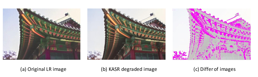
Figure 1: The image in (c) highlights (in pink) the differences between the original low-resolution image in (a) and the LR image down-sampled by the proposed model in (b). Notice that the differences are mainly due to color changes combined with some texture distortions.

In this paper, we introduce a generic framework to better represent the real-world image super-resolution process, named Kernel Adversarial Learning Super-Resolution (KASR). KASR can adversarially generate degradation kernels and inject noises, but without requiring prior knowledge of the kernels or noises. It is designed to allow a seamless integration with many mainstream SR models. The LR images generated by KASR and the differences with the original LR ones are shown in Figure 1. Furthermore, we introduce an optimisation process named Iterative Supervision to gradually refine the SR images. Also, a high-frequency selective loss function is proposed to further force the model to attend to high-frequency areas within SR images. Experimental results demonstrate that, when compared to multiple strong baselines on real-world datasets, mainstream SR models equipped with KASR are able to generate high-quality SR images in real-world scenarios. Our contributions are summarised as follows:

• We propose the KASR framework from an adversarial training perspective to deal with the real-world image super-resolution task. The proposed framework is able to model the image degradation process implicitly (i.e., without explicitly specifying kernels and noises [15]) by exploring an end-to-end training of neural networks.

• To effectively utilise existing supervision signals, we introduce the Iterative Supervision optimisation process to gradually refine the SR image.

• Given the need of SR models to focus on high-frequency areas of the image, we design a high-frequency selective objective function to assign more attention to high-frequency regions of the images during the minimisation of the super-resolution reconstruction error.

We show extensive experiments which demonstrate that mainstream SR models equipped with KASR achieve superior performance over competitive methods across two real-world datasets.

II Related Work

II-A Real-world Image Super-resolution

Low-resolution images can be viewed as degraded high-resolution images after blurring, down-sampling and noise interference. An important premise of deep learning, and machine learning in general, is that the distribution from which test images are drawn is the same as the distribution used to generate the training data. When the naive degradation process in the training phase is inconsistent with the degradation process in real-world images, the SR result will not be accurate. Therefore, the simulation of a real-world complex degradation process is crucial.

Gaussian kernel is the most widely adopted blur kernel [16, 17], but it differs from real-world blur kernels significantly. Therefore, some papers attempted to simulate the degradation process in a more complicated manner by considering a variety of degradation kernels and noise levels. Zhang et al.[18] examine the performance of SR models under a set of Gaussian blur kernels and receives different results under different kernel assumptions. Another typical idea is to estimate a finite set of down-sampling kernels/noises and inject them into training images as [15]. However, such finite set of kernels and noises still represent a strong assumption.

Approaching the problem from a few-shot learning perspective, Shocher et al.[14] proposed a kernel estimation approach by further down-sampling the given low-resolution image and learning a super-resolution function from these low-high resolution image pairs. However, this method is not practical to be applied directly in the inference phase since training is required on each test image, which is time-consuming. A similar idea has been adopted by KernelGAN [13]. Nevertheless, in the models above, the unrealistic assumption of Gaussian blur kernels still exists in model training.

II-B Adversarial Training

As shown in [19], deep neural network models are very sensitive to small perturbations of the inputs. In particular, tiny pixel-wise distortions can lead deep neural networks to produce entirely different results. This issue can be mitigated with adversarial training that trains models to be robust against attacks formed by dynamically and adaptively adding perturbations to the training samples.

In real-world SR scenarios, models usually suffer from poor generalisation performance due to unknown degradation kernels and noise in the inference phase. Furthermore, non-additive noise can be injected by different CMOS image sensors. Although GANs [6, 20] have been introduced in SR to serve as objective functions to generate more photo-realistic images, they were used in a different context from what we are exploring. In our paper, we adopt adversarial training to model unknown kernels and non-additive noises. To the best of our knowledge, we are the first to introduce adversarial training into the SR task for end-to-end implicit simulation of the degradation process without extra training.

III The Proposed Method

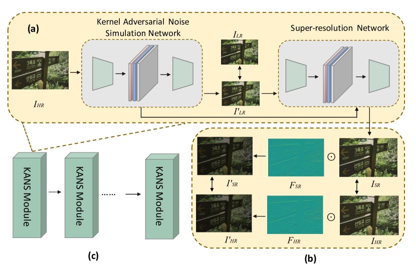
Figure 2: The overall framework of the proposed KASR framework. The framework consists of three parts: (a) the Kernel Adversarial Noise Simulation (KANS) to adaptively simulate the image degradation process; (b) the High-frequency Selective Objective to force the model to focus on high-frequency regions within images due to the higher importance placed in the image regions containing high-frequency for the SR task; and (c) the stacking of multiple KANS modules, where the Iterative Supervision (IS) can leverage the supervision signals to accurately refine the SR image reconstruction.

III-A Overall Framework

The proposed KASR framework is divided into three parts: the Kernel Adversarial Noise Simulation (KANS) to implicitly and dynamically simulate the image degradation process for robust SR model training; the High-frequency Selective Objective (HFSO) to constrain the model to focus on high-frequency regions of the images; and the Iterative Supervision (IS) to leverage the provided supervision signals in a better manner by repeatedly stacking KANS modules for SR reconstruction refinement. These parts are designed to complement each other and to be combined seamlessly with mainstream SR models.

High-frequency Selective Objective. As shown in Figure 2, a high-resolution image $I_{HR}$ is fed into the KANS network to generate a low-resolution image $I^{\prime}_{LR}$ perturbed with non-additive noises. We constrain the $I^{\prime}_{LR}$ to be visually similar to the original low-resolution image $I_{LR}$, but the injected perturbations will try to interfere with the downstream super-resolution image restoration process by maximising the super-resolution loss. After the super-resolution image is generated, the HFSO constrains the model to focus on the high-frequency regions of the images since an accurate reconstruction in those regions is crucial for a reliable SR model. In HFSO, we extract high-frequency maps from the HR and SR images and normalise them to be in the range $[0,1]$ to form the high-frequency attention masks. Next, we apply the Hadamard product between the high-frequency attention masks and the HR/SR images to get the high-frequency filtered images. Moreover, the IS iteratively refines the results.

Iterative Supervision. In standard SR models, high-resolution images are directly generated from low-resolution images. Different from that, we propose to perform iterative optimisation by repeating the degradation and the super-resolution processes. The ground-truth high-resolution images will be used to train each KANS module. The gradients are able to flow all the way back through the chain by providing supervision to the iteratively generated images. Therefore, supervision signals can be more effectively used to better supervise the super-resolution process.

III-B Kernel Adversarial Noise Simulation

In this section, we propose the Kernel Adversarial Noise Simulation (KANS) module. Adversarial training techniques were initially proposed to defend against adversarial attacks [19, 21]. However, in the context of real-world SR, we adopt adversarial training to actively generate adaptive blur kernels and non-trivial simulated noises to be injected into the low-resolution image with the goals of reconstructing well the low resolution image and adversarially reconstructing the super-resolution image. This problem is formulated as an optimisation problem to search for the suitable blur kernel $k$ and noise $\delta$ subject to get the optimal parameters $\theta_{\eta}^{*}$ for super-resolution. This optimisation is a minimisation maximisation problem that adversarially reconstructs the super-resolution image, as follows:

$$\begin{split}\min_{k,\delta}\;\;\;&\|((I_{HR}\ast k)\!\downarrow_{\bf{s}}+\delta)-I_{LR}\|_{p}-\\ &\|\eta((I_{HR}\ast k)\!\downarrow_{\bf{s}}+\delta;\theta_{\eta}^{*})-I_{HR}\|_{p}\\ s.t.\;\;\;&\theta_{\eta}^{*}=\operatorname*{arg\,min}\|\eta((I_{HR}\ast k)\!\downarrow_{\bf{s}}+\delta;\theta_{\eta})-I_{HR}\|_{p},\end{split}$$ (2)

where $s$ is the scale, $(I_{HR}\ast k)\!\downarrow_{\bf{s}}$ is the degradation process, $\eta(\cdot)$ is the super-resolution function parameterised by $\theta_{\eta}$, and $||\cdot||_{p}$ denotes the p-norm operator. In super-resolution, the direct optimization of Equation 2 is not trivial because we need to define an appropriate domain for the kernel and the noise optimisation can be computationally expensive. Alternatively, we propose to solve this optimisation by adopting neural networks to directly generate the degradation kernel and the noise to down-sampled images, such that the noise can be generated dynamically with little computational increment. Hence, the optimisation from Equation 2 can be re-formulated as the following two-step optimization:

where the $\phi(\cdot)$ is the degradation neural network function with parameter $\theta_{\phi}$. By doing so, complex blur kernels and highly non-additive noises can be injected into the generated low-resolution image. More specifically, as mentioned above, a data-driven approach is adopted to solve the non-additive blur kernel and noise injection problem by minimising the reconstruction error over the generated and real low-resolution image pairs but maximising the super-resolution image restoration error.

III-C Objective Functions

In the super-resolution task, high-frequency (HF) areas of an image ought to be explored more than low-frequency (LF) areas to improve the reconstruction quality. Naive pixel-wise losses (e.g., MSE objective) assign the same weight to each pixel, independently if it is part of a low or high-frequency region, and average the errors that come from these pixels. Inevitably, this strategy will result in blurred SR image reconstruction because images tend to have a disproportionally larger amount of LF regions than of HF regions, so these LF regions will be better reconstructed than the HF areas, resulting in such blurred reconstruction. Thus, pixels should be assigned with different weights depending if they lie in an LF or HF region of the image for SR tasks. Due to the imbalanced distribution of HF and LF regions, pixels located in HF regions require more attention. Therefore, we adopt the HFSO to attend more to the HF regions within an image. Formally, the HFSO is represented as:

$$L_{HFSO}(\theta_{\eta})=\|\psi(f(I_{HR}))\odot I_{HR}-\psi(f(I_{SR}))\odot I_{SR}\|_{p},$$ (4)

where the super-resolution image $I_{SR}=\eta(\phi(I_{HR};\theta_{\phi});\theta_{\eta})$ has the same dimensions as $I_{HR}$, $f(\cdot)$ is the high-frequency filter, $\psi(\cdot)$ denotes the normalisation operator, and $\odot$ represents the element-wise Hadamard product. Similar to Equation (3), $p$-norm is performed in the Equation (4).

Besides the aforementioned objectives of KANS and HFSO, the pixel-wise super-resolution reconstruction objective has been adopted:

$$L_{REC}(\theta_{\eta})=\|I_{SR}-I_{HR}\|_{p},$$ (5)

where $I_{SR}$ is defined in Equation (4).

Therefore, the total objective function for the super-resolution network is:

$$L_{SR}(\theta_{\eta})=L_{REC}(\theta_{\eta})+\omega L_{HFSO}(\theta_{\eta}),$$ (6)

where $\omega$ is the trade-off factor between this two objectives. From the adversarial training perspective, besides the Equation 3, a discriminative objective $L_{d}$ is also adopted to train a discriminator to classify the original and generated LR images into real or fake. This is designed to further ensure the visual quality of the generated images. So the overall objective for KANS can be presented as:

$$L_{KANS}(\theta_{\phi})=\|I^{\prime}_{LR}-I_{LR}\|_{p}-\beta\|I_{SR}-I_{HR}\|_{p}+\gamma L_{d},$$ (7)

where $I^{\prime}_{LR}=\phi(I_{HR};\theta_{\phi})$, $\beta$ and $\gamma$ are weight factors to balance the three terms. The training process of KASR can be found in Algorithm 1.

Input: Low-resolution image $I_{LR}$, degradation neural network parameter $\theta_{\phi}$, super-resolution network parameter $\theta_{\eta}$, number of KANS Modules $N$ for iterative supervision, and learning rate $\alpha$

Output: Super-resolution image $I_{SR}$

Initialize model parameters $\theta_{\phi}$ and $\theta_{\eta}$

while training has not converged do

       $I_{SR}\leftarrow I_{HR}$

       for n=1 to N do

             Generate LR image $I^{\prime}_{LR}=\phi(I_{SR};\theta_{\phi})$

             Evaluate loss $L_{KANS}(\theta_{\phi})=||I^{\prime}_{LR}-I_{LR}||_{p}-\beta\|I_{SR}-I_{HR}\|_{p}+\gamma L_{d}$

             Update $\theta_{\phi}\leftarrow\theta_{\phi}-\alpha\nabla_{\theta_{\phi}}L_{KANS}(\theta_{\phi})$

              

             Generate SR image $I_{SR}=\eta(I^{\prime}_{LR};\theta_{\eta})$

             Evaluate loss $L_{SR}(\theta_{\eta})=\|I_{SR}-I_{HR}\|_{p}+\omega\|\psi(f(I_{HR}))\odot I_{HR}-\psi(f(I_{SR}))\odot I_{SR}\|_{p}$

             Update $\theta_{\eta}\leftarrow\theta_{\eta}-\alpha\nabla_{\theta_{\eta}}L_{SR}(\theta_{\eta})$

       end for

      

end while

Algorithm 1 The training process of KASR

IV Experiments

In the experiments, we examine the effectiveness of the proposed KASR framework combined with multiple mainstream super-resolution models on two real-world datasets. Then, comparisons between the proposed model with existing SR models are performed. In the ablation study, the effectiveness of each component is validated.

IV-A Experimental Setup

Evaluation measures. We adopt Peak Signal to Noise Ratio (PSNR) [16] and Structural Similarity (SSIM) [22] as our evaluation measures. Moreover, since PSNR and SSIM only take pixel-wise distance into consideration, we further include the widely adopted Learned Perceptual Image Patch Similarity (LPIPS) [23] for perceptual evaluation. LPIPS aims to emulate human observations by depicting the perceptual similarities between SR images and real HR ones.

Datasets. We conduct model training and evaluation on two real-world image SR datasets, namely: RealSR [24] (including both $\times 2$ and $\times 4$ super-resolution) and City100 [25] ($\times 3$ super-resolution). In the RealSR dataset, there are 506 and 500 low-resolution/high-resolution image pairs taken by Canon and Nikon cameras for $\times 2$ and $\times 4$ up-scaling, respectively. From RealSR dataset, we adopt 406 images for $\times 2$ model training and 400 images for $\times 4$ model training. The remaining 100 images for each case are useed for model testing. The City100 dataset contains 100 real-world low-resolution/high-resolution image pairs taken by a Nikon camera with $\times 3$ up-scaling. We adopt the first 95 images for model training and the remaining 5 images for model evaluation.

Implementation details. During the training of models, batches of size 32 are adopted, and Adam optimizer is chosen for model optimization. Following the setup by Lim et al. [4], we randomly flip images vertically/horizontally and rotate them by 90 degrees for data augmentation. The initial learning rate is set to $10^{-4}$. The models are trained for 300 epochs with a multi-step learning rate reduction strategy. The hyper-parameter $\omega$ to compute $L_{SR}(\theta_{\eta})$ in Equation (6) is set to 0.5; $\beta$ to compute $L_{KANS}(\theta_{\phi})$ in Equation (7) is set to 1.0; and $\gamma$, also in in Equation (7), is set to 0.5. For the implementation of the KANS Network, three convolutional layers are combined with the LeakyReLU activation function and Max-pooling operation, where $2\times 10^{-1}$ is selected as the negative slope of LeakyReLU activation. 32 neural units are set for each hidden layer of the KANS Network. In the experiments, the $p$-norm in all losses for the KANS module are defined as the $L_{1}$ norm, and we use $N=2$ KANS modules for the iterative supervision training. We use the Sobel filter as the high-frequency filter $f(\cdot)$ and min-max normalisation as $\psi(\cdot)$ in Equation (4). By default, the model labelled as ’Ours’ in the experiments below consists of our proposed KASR paired with the EDSR model [4]. The models are implemented with PyTorch and trained/tested on one NVIDIA GTX 1080 Ti graphic card. The experimental settings are kept the same across all experiments for fair comparisons.

IV-B Overall Performance

We compare the proposed model with existing super-resolution models. Following the mainstream evaluation of SR models [4], we present our model performance with self-ensemble [26], which forms the model Ours+, to further enhance the model performance. During the evaluation of Ours+, instead of inputting a single low-resolution image, we augment it to produce seven images using different rotations, which together with the original image are processed the SR model. After getting the corresponding SR images and rotating the images back to original angles, pixel-level weighted average is performed to obtain the final SR result. The experiments are conducted on RealSR dataset (both $\times 2$ and $\times 4$ up-scalings) and City100 dataset, and results are shown in Tables I, II, and III.

TABLE I: The comparison of our proposed model and existing super-resolution models on RealSR dataset with $\times 2$ up-scaling. The best results per column are bolded, $\uparrow$ indicates that larger is better and $\downarrow$ shows that lower is better.

Methods	Scale	PSNR $\uparrow$	SSIM $\uparrow$	LPIPS $\downarrow$
Bicubic	$\times 2$	30.270	0.874	0.210
ZSSR [14]	$\times 2$	30.563	0.879	0.176
KernelGAN [13]	$\times 2$	30.240	0.891	0.134
MZSR [27]	$\times 2$	27.960	0.816	0.211
DBPI [28]	$\times 2$	27.860	0.829	0.178
DAN [29]	$\times 2$	30.630	0.882	0.131
SRResCGAN [30]	$\times 2$	26.260	0.798	0.209
FSSR [31]	$\times 2$	30.397	0.874	0.142
DASR [32]	$\times 2$	29.887	0.867	0.129
CinCGAN [33]	$\times 2$	28.099	0.867	0.166
ESRGAN [6]	$\times 2$	30.648	0.880	0.097
Ours	$\times 2$	32.454	0.922	0.080
Ours+	$\times 2$	32.519	0.923	0.082

TABLE II: The comparison of our proposed model and existing super-resolution models on RealSR dataset with $\times 4$ up-scaling. The best results per column are bolded, $\uparrow$ indicates that larger is better and $\downarrow$ shows that lower is better.

Methods	Scale	PSNR $\uparrow$	SSIM $\uparrow$	LPIPS $\downarrow$
Bicubic	$\times 4$	25.740	0.741	0.467
ZSSR [14]	$\times 4$	26.007	0.748	0.386
KernelGAN [13]	$\times 4$	24.090	0.724	0.298
DBPI [28]	$\times 4$	22.360	0.656	0.311
DAN [29]	$\times 4$	26.200	0.760	0.410
IKC [34]	$\times 4$	25.600	0.749	0.319
SRResCGAN [30]	$\times 4$	25.840	0.746	0.375
FSSR [31]	$\times 4$	25.992	0.739	0.265
DASR [32]	$\times 4$	26.782	0.782	0.228
CinCGAN [33]	$\times 4$	25.094	0.746	0.405
ESRGAN [6]	$\times 4$	27.569	0.774	0.415
RCAN [5]	$\times 4$	27.647	0.780	0.442
Noise-injection [15]	$\times 4$	25.768	0.772	0.215
Ours	$\times 4$	27.850	0.824	0.148
Ours+	$\times 4$	27.991	0.827	0.150

We compare our results with the results by multiple state-of-the-art super-resolution methods obtained from [35] and [32] in Tables I and  II. The competing methods are: naive Bicubic up-sampling; ZSSR [14] and KernelGAN [13] that are degradation estimation models performed on testing data; MZSR [27] that combines Zero-Shot Learning and Meta Transfer Learning; DBPI [28] which is a unified internal learning-based super-resolution model; DAN [29] that separates the kernel estimation and restoration as two sub-steps; IKC [34] which iteratively conducts kernel correction; SRResCGAN [30] that introduces generative adversarial residual CNN into Real-World Super-Resolution domain; FSSR [31] that considers low frequency and high frequency separately for real super-resolution images; DASR [32] which adopts domain-gap aware training strategy and domain-distance weighted supervision; CinCGAN [33] that represents Cycle-in-Cycle GAN to use domain translation in real SR domain; ESRGAN [6] and RCAN [5] which are two of the most popular models, where ESRGAN is an upgraded version of SRGAN based on the introduction of a residual-in-residual dense block and a new structure, and RCAN proposed a very deep residual network architecture for SR tasks; and the Noise-injection model [15] that is a baseline real-world super-resolution model. The noise-injection model estimates a finite set of degradation kernels and noises from pre-collected real images by adopting KernelGAN [13] and ZSSR [14]. In order to deal with real-world SR noises, the noise-injection model performs a degradation operation from the degradation pool during training. However, extra training time for kernel collection is required.

On the RealSR results from Tables I and II, our model outperforms competing approaches by a large margin for all three measures, especially on LPIPS evaluations. The DASR model and Noise-injection model have better perceptual results than other competing models, but they are still not as good as our model. On $\times 4$ scaling, compared with the DASR model, the LPIPS obtained by our KASR model is 35% better. Compared with the Noise-injection model, our model improves the LPIPS measure from 0.215 to 0.148.

TABLE III: The comparison of our proposed model and existing super-resolution models on City100 dataset with $\times 3$ up-scaling. The best results of a column are bolded, $\uparrow$ indicates that larger is better and $\downarrow$ shows that lower is better.

Methods	Scale	PSNR $\uparrow$	SSIM $\uparrow$	LPIPS $\downarrow$
RCAN [5]	$\times 3$	28.114	0.811	0.384
RCAN* [5]	$\times 3$	30.016	0.864	0.260
CinCGAN [33]	$\times 3$	26.221	0.703	0.303
CamSR-SRGAN [25]	$\times 3$	25.257	0.764	0.195
CamSR-VDSR [25]	$\times 3$	30.260	0.868	0.263
Ours	$\times 3$	30.714	0.824	0.112
Ours+	$\times 3$	30.831	0.827	0.113

Similar results are shown in Table III on City100 dataset. The competing methods include RCAN and RCAN* [5], where RCAN* is trained with real low-resolution and high-resolution pairs; CinCGAN [33]; CamSR-SRGAN [25] and CamSR-VDSR [25] which are two variants of CameraSR model based on SRGAN and VDSR. Our model improves the PSNR value from 30.260 to 30.714, compared to the second best model CamSR-VDSR. When compared with CamSR-based models, the proposed model improves the LPIPS measure by a large margin.

Interestingly, from these tables, we can verify that models with self-ensemble (Ours+ models) are able to boost performance for both PSNR and SSIM, but not for LPIPS. This can be because the self-ensemble operation performs a pixel-level ensemble that may not effectively increase the perceptual quality of the images.

IV-C Ablation Study

Experiments on RealSR. We equip the proposed KASR framework on three modern super-resolution models, namely: EDSR [4], SRResNet [3] and SRGAN [3]. From Table IV, we can see that the models equipped with KASR are able to consistently obtain better results, when compared with the original models. Under $\times 2$ up-scaling, SRResNet-KASR increases PSNR by 0.322 compared with the original SRResNet model. SRGAN-KASR also increases the PSNR result by 0.301. For $\times 4$ up-scaling, EDSR-KASR increases the PSNR results of the EDSR model from 27.494 to 27.850 and SSIM from 0.813 to 0.824. Similarly, we notice a PSNR improvement of 0.294 for the SRResNet-KASR model and 0.279 for the SRGAN-KASR model. The performance improvements are not only for the pixel-level evaluation measures (PSNR and SSIM) since the models equipped with KASR are able to produce better results on the perceptual measure LPIPS as well. Empirically, we also notice that SSIM scores are generally more consistent across all models than PSNR results. Only on $\times 4$ setting, the SRGAN with KASR model is slightly worse than the baseline in terms of SSIM, but it performs better on the perceptual measure LPIPS, possibly because GAN-based models are generally able to capture the semantic information of images than non-GAN models in a better manner.

TABLE IV: The comparison between original models and the ones equipped with the proposed KASR framework on RealSR dataset with $\times 2$ and $\times 4$ up-scaling.

Methods	Scale	PSNR $\uparrow$	SSIM $\uparrow$	LPIPS $\downarrow$
EDSR [4]	$\times 2$	32.378	0.922	0.081
EDSR-KASR (Ours)	$\times 2$	32.454	0.922	0.080
SRResNet [3]	$\times 2$	31.630	0.915	0.086
SRResNet-KASR (Ours)	$\times 2$	31.952	0.915	0.083
SRGAN [3]	$\times 2$	31.611	0.915	0.086
SRGAN-KASR (Ours)	$\times 2$	31.912	0.915	0.081
EDSR [4]	$\times 4$	27.494	0.813	0.157
EDSR-KASR (Ours)	$\times 4$	27.850	0.824	0.148
SRResNet [3]	$\times 4$	27.366	0.819	0.153
SRResNet-KASR (Ours)	$\times 4$	27.660	0.820	0.153
SRGAN [3]	$\times 4$	27.355	0.819	0.156
SRGAN-KASR (Ours)	$\times 4$	27.634	0.818	0.151

Experiments on City100. Similarly, we equip the KASR framework on EDSR [4], SRResNet [3] and SRGAN [3] for the City100 experiment. The quantitative comparisons are shown on Table V. On the City100 dataset, a 0.743 PSNR increment is obtained by the EDSR-KASR model. We find from this table that the perceptual performance improvements of the model equipped with the KASR framework are clearer on City100 than on RealSR. For instance, on City100, EDSR-KASR improves the LPIPS measure from 0.138 to 0.112; both SRResNet-KASR and SRGAN-KASR improve the LPIPS measure from 0.117 to 0.109. This phenomenon may be caused by the different distribution of data in different datasets.

TABLE V: The comparison between original models and the ones equipped with the proposed KASR framework on City100 dataset with $\times 3$ up-scaling.

Methods	Scale	PSNR $\uparrow$	SSIM $\uparrow$	LPIPS $\downarrow$
EDSR [4]	$\times 3$	29.971	0.765	0.138
EDSR-KASR (Ours)	$\times 3$	30.714	0.824	0.112
SRResNet [3]	$\times 3$	30.305	0.817	0.117
SRResNet-KASR (Ours)	$\times 3$	30.309	0.816	0.109
SRGAN [3]	$\times 3$	30.181	0.815	0.117
SRGAN-KASR (Ours)	$\times 3$	30.253	0.815	0.109

Effect of different components. This section examines the contribution of different components of the proposed KASR framework, including the Kernel Adversarial Noise Simulation network (KANS), High-frequency Selective Objective (HFSO) and Iterative Supervision (IS). The quantitative results are shown in the Table VI. Starting from the backbone model EDSR in model #1, we add KANS to build model #2, which improves PSNR from 27.494 to 27.718; SSIM from 0.813 to 0.823; LPIPS from 0.157 to 0.151. By introducing HFSO and IS, the performance of the model can be further boosted to our best model #4 with 27.850 on PSNR, 0.824 on SSIM and 0.148 on LPIPS. It is worth noting that the KANS module in model #2 contributes the most to improve the results, producing better results on pixel-level measures (PSNR and SSIM) and the perceptual measure (LPIPS) than model #1. HFSO and IS also show to further boost model performance.

TABLE VI: Ablation study of each proposed component. The experiments are conducted on the RealSR dataset with $\times 4$ up-scaling. The backbone model is EDSR.

Model #	KANS	HFSO	IS	PSNR $\uparrow$	SSIM $\uparrow$	LPIPS $\downarrow$
1				27.494	0.813	0.157
2	✓			27.718	0.823	0.151
3	✓	✓		27.762	0.823	0.151
4	✓	✓	✓	27.850	0.824	0.148

IV-D Analysis

Number of KANS Modules. We conduct experiments to examine the number of KANS modules for Iterative Supervision (IS) on Table VII. We notice that there is a general trend of evaluation measures improving and then decreasing with a growing number of KANS modules. When number of KANS modules is 2, the performance reaches the peak.

TABLE VII: The examination of the number of KANS modules for Iterative Supervision (IS). The experiments are conducted on the RealSR dataset with $\times 4$ up-scaling and the backbone model is EDSR.

KANS modules #	PSNR $\uparrow$	SSIM $\uparrow$	LPIPS $\downarrow$
1	27.762	0.823	0.151
2	27.850	0.824	0.148
3	27.764	0.823	0.148

High-frequency Selective Objective Versus High-frequency loss only. We perform a comparison between the proposed HFSO objective and the loss HF-only computed using only the high-frequency maps of generated SR images and ground-truth images without the element-wise product with the image shown in Equation (4). From Table VII, the model trained with HFSO shows better results across the three evaluation measures when compared to HF-loss only. In particular, compared with the HF-only, HFSO increases PSNR from 27.734 to 27.850 and LPIPS from 0.153 to 0.148. The HFSO objective works more effectively than HF-only since it softly weights pixels which enables a richer information content than just using the HF maps.

TABLE VIII: The comparison of the proposed HFSO objective versus high-frequency loss only. The experiments are conducted on the RealSR dataset with $\times 4$ up-scaling and the backbone model is EDSR.

Objective	PSNR $\uparrow$	SSIM $\uparrow$	LPIPS $\downarrow$
HF-only	27.734	0.821	0.153
HFSO	27.850	0.824	0.148

Sensitivity of $L_{KANS}(\theta_{\phi})$ to $\beta$ in Equation (7). The factor $\beta$ in Equation (7) controls the intensity of adversarial training when computing $L_{KANS}(\theta_{\phi})$, thus playing an important role in the model performance. Table IX shows the model sensitivity to $\beta$. The experiments are conducted on the RealSR dataset with $\times 4$ up-scaling and backbone model EDSR. It is interesting to note that the results show that our model has a rather stable performance as a function of $\beta$ in terms of PSNR, SSIM and LPIPS measures. It is also worth noting that all results show a slight improvement with the increase of $\beta$. In general, we suggest the use of $\beta=1.0$ to obtain the results shown in this paper.

TABLE IX: Sensitivity of $L_{KANS}(\theta_{\phi})$ to $\beta$ in Equation (7) on the RealSR dataset with $\times 4$ up-scaling and backbone model EDSR.

$\beta$	PSNR $\uparrow$	SSIM $\uparrow$	LPIPS $\downarrow$
$\beta$ = 0.1	27.722	0.823	0.150
$\beta$ = 0.3	27.768	0.824	0.149
$\beta$ = 0.5	27.829	0.824	0.150
$\beta$ = 0.7	27.795	0.824	0.150
$\beta$ = 1.0	27.850	0.824	0.148

Sensitivity of $L_{KANS}(\theta_{\phi})$ to $\gamma$ in Equation (7). We also examine the sensitivity of our method to $\gamma$ in Equation (7), which is the weight of the discriminant loss to classify the original and generated LR images into real or fake. As shown in Table X, the model’s performance is quite stable with respect to $\gamma$, with a slight upward trend for $\gamma\in[0.1,0.5]$ followed by a downward trend for $\gamma\in[0.7,1.0]$. Hence, $\gamma=0.5$ shows the peak performance, so we recommend $\gamma=0.5$.

TABLE X: Sensitivity of $L_{KANS}(\theta_{\phi})$ to $\gamma$ in Equation (7) on the RealSR dataset with $\times 4$ up-scaling and backbone model EDSR.

$\gamma$	PSNR $\uparrow$	SSIM $\uparrow$	LPIPS $\downarrow$
$\gamma$ = 0.1	27.730	0.822	0.151
$\gamma$ = 0.3	27.781	0.823	0.149
$\gamma$ = 0.5	27.850	0.824	0.148
$\gamma$ = 0.7	27.802	0.823	0.149
$\gamma$ = 1.0	27.801	0.822	0.151

Visualization of generated LR images from KANS. Figures 3(a)-(e) show comparisons of original low-resolution images $I_{LR}$ and KANS-generated low-resolution images $I^{\prime}_{LR}$. The distortions include texture changes, colour modifications and blur. As shown in the figure, $I_{LR}$ and $I^{\prime}_{LR}$ are visually similar, but small perturbations are present in $I^{\prime}_{LR}$ to mislead deep super-resolution models. In (a), $I^{\prime}_{LR}$ shows changes in terms of colour and texture when compared with $I_{LR}$. In (b), texture modifications are shown in $I^{\prime}_{LR}$. In (c), colour changes are displayed on $I^{\prime}_{LR}$. In (d), blur is shown in $I^{\prime}_{LR}$ compared with $I_{LR}$. In (e), some fine details are added to $I^{\prime}_{LR}$.

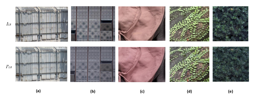
Figure 3: Illustration of the differences between original images $I_{LR}$ and KASR produced images $I^{\prime}_{LR}$.

Visualization of SR images. From the visualization in Figure 4, we notice that the proposed model KASR can generate clearer SR images than the Bicubic method and RCAN model in real-world image scenarios. Similar results are shown in Figure 5, where our KASR model shows clearer SR images than the competitors. It is worth noting that the Noise-injection model [15] can generate clear SR images in some cases, but it can create small artifacts as the character and the man’s beard shown in the figures. This may be because its estimated kernels and noises cannot cover all the real degradation kernels.

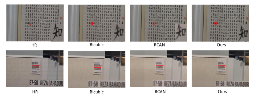
Figure 4: Visual comparison between the original HR image, Bicubic interpolation, RCAN and our proposed KASR model.

Figure 5: Visual comparison between the original HR image, Bicubic interpolation, Noise-injection and the proposed model.

V Conclusion

In this paper, we proposed the Kernel Adversarial Learning Super-resolution (KASR) to assist SR models to implicitly simulate the complex image degradation process. Besides, an iterative supervision process and a high-frequency selective objective were also proposed to further boost the model performance. The experiments combining KASR with three SR models indicated that our proposed framework can be equipped into modern SR models seamlessly. Promising results are shown in real-world SR scenarios by KASR when compared with other models. Furthermore, an extensive ablation study was performed to examine the effectiveness of each component of the proposed framework. From the visualization of SR images, the proposed approach is able to generate clear SR images compared with its competitors.

References

- [1] C. Dong, C. C. Loy, K. He, and X. Tang, “Image super-resolution using deep convolutional networks,” IEEE transactions on pattern analysis and machine intelligence, vol. 38, no. 2, pp. 295–307, 2015.
- [2] J. Kim, J. Kwon Lee, and K. Mu Lee, “Accurate image super-resolution using very deep convolutional networks,” in Proceedings of the IEEE conference on computer vision and pattern recognition, 2016, pp. 1646–1654.
- [3] C. Ledig, L. Theis, F. Huszár, J. Caballero, A. Cunningham, A. Acosta, A. Aitken, A. Tejani, J. Totz, Z. Wang et al., “Photo-realistic single image super-resolution using a generative adversarial network,” in Proceedings of the IEEE conference on computer vision and pattern recognition, 2017, pp. 4681–4690.
- [4] B. Lim, S. Son, H. Kim, S. Nah, and K. Mu Lee, “Enhanced deep residual networks for single image super-resolution,” in Proceedings of the IEEE conference on computer vision and pattern recognition workshops, 2017, pp. 136–144.
- [5] Y. Zhang, K. Li, K. Li, L. Wang, B. Zhong, and Y. Fu, “Image super-resolution using very deep residual channel attention networks,” in Proceedings of the European Conference on Computer Vision (ECCV), 2018, pp. 286–301.
- [6] X. Wang, K. Yu, S. Wu, J. Gu, Y. Liu, C. Dong, Y. Qiao, and C. Change Loy, “Esrgan: Enhanced super-resolution generative adversarial networks,” in Proceedings of the European Conference on Computer Vision (ECCV), 2018, pp. 0–0.
- [7] Z. Wang, J. Chen, and S. C. Hoi, “Deep learning for image super-resolution: A survey,” IEEE transactions on pattern analysis and machine intelligence, vol. 43, no. 10, pp. 3365–3387, 2020.
- [8] H. Tian, B. Fowler, and A. E. Gamal, “Analysis of temporal noise in cmos photodiode active pixel sensor,” IEEE Journal of Solid-State Circuits, vol. 36, no. 1, pp. 92–101, 2001.
- [9] C. Liu, W. T. Freeman, R. Szeliski, and S. B. Kang, “Noise estimation from a single image,” in IEEE Conf. Comput. Vis. Pattern Recog., vol. 1. IEEE, 2006, pp. 901–908.
- [10] C. Liu, R. Szeliski, S. B. Kang, C. L. Zitnick, and W. T. Freeman, “Automatic estimation and removal of noise from a single image,” IEEE transactions on pattern analysis and machine intelligence, vol. 30, no. 2, pp. 299–314, 2007.
- [11] J. Kim, J. Kwon Lee, and K. Mu Lee, “Deeply-recursive convolutional network for image super-resolution,” in Proceedings of the IEEE conference on computer vision and pattern recognition, 2016, pp. 1637–1645.
- [12] W. Shi, J. Caballero, F. Huszár, J. Totz, A. P. Aitken, R. Bishop, D. Rueckert, and Z. Wang, “Real-time single image and video super-resolution using an efficient sub-pixel convolutional neural network,” in Proceedings of the IEEE conference on computer vision and pattern recognition, 2016, pp. 1874–1883.
- [13] S. Bell-Kligler, A. Shocher, and M. Irani, “Blind super-resolution kernel estimation using an internal-gan,” arXiv preprint arXiv:1909.06581, 2019.
- [14] A. Shocher, N. Cohen, and M. Irani, ““zero-shot” super-resolution using deep internal learning,” in Proceedings of the IEEE Conference on Computer Vision and Pattern Recognition, 2018, pp. 3118–3126.
- [15] X. Ji, Y. Cao, Y. Tai, C. Wang, J. Li, and F. Huang, “Real-world super-resolution via kernel estimation and noise injection,” in IEEE Conf. Comput. Vis. Pattern Recog. Workshops, 2020, pp. 466–467.
- [16] C.-Y. Yang, C. Ma, and M.-H. Yang, “Single-image super-resolution: A benchmark,” in European conference on computer vision. Springer, 2014, pp. 372–386.
- [17] W. Dong, L. Zhang, G. Shi, and X. Li, “Nonlocally centralized sparse representation for image restoration,” IEEE transactions on Image Processing, vol. 22, no. 4, pp. 1620–1630, 2012.
- [18] K. Zhang, L. V. Gool, and R. Timofte, “Deep unfolding network for image super-resolution,” in Proceedings of the IEEE/CVF Conference on Computer Vision and Pattern Recognition, 2020, pp. 3217–3226.
- [19] I. J. Goodfellow, J. Shlens, and C. Szegedy, “Explaining and harnessing adversarial examples,” arXiv preprint arXiv:1412.6572, 2014.
- [20] H. Ren, A. Kheradmand, M. El-Khamy, S. Wang, D. Bai, and J. Lee, “Real-world super-resolution using generative adversarial networks,” in Proceedings of the IEEE/CVF Conference on Computer Vision and Pattern Recognition Workshops, 2020, pp. 436–437.
- [21] F. Tramèr, A. Kurakin, N. Papernot, I. Goodfellow, D. Boneh, and P. McDaniel, “Ensemble adversarial training: Attacks and defenses,” arXiv preprint arXiv:1705.07204, 2017.
- [22] Z. Wang, A. C. Bovik, H. R. Sheikh, and E. P. Simoncelli, “Image quality assessment: from error visibility to structural similarity,” IEEE transactions on image processing, vol. 13, no. 4, pp. 600–612, 2004.
- [23] R. Zhang, P. Isola, A. A. Efros, E. Shechtman, and O. Wang, “The unreasonable effectiveness of deep features as a perceptual metric,” in IEEE Conf. Comput. Vis. Pattern Recog., 2018, pp. 586–595.
- [24] J. Cai, H. Zeng, H. Yong, Z. Cao, and L. Zhang, “Toward real-world single image super-resolution: A new benchmark and a new model,” in IEEE Conf. Comput. Vis. Pattern Recog., 2019, pp. 3086–3095.
- [25] C. Chen, Z. Xiong, X. Tian, Z.-J. Zha, and F. Wu, “Camera lens super-resolution,” in IEEE Conf. Comput. Vis. Pattern Recog., 2019, pp. 1652–1660.
- [26] R. Timofte, R. Rothe, and L. Van Gool, “Seven ways to improve example-based single image super resolution,” in Proceedings of the IEEE conference on computer vision and pattern recognition, 2016, pp. 1865–1873.
- [27] J. W. Soh, S. Cho, and N. I. Cho, “Meta-transfer learning for zero-shot super-resolution,” in Proceedings of the IEEE/CVF Conference on Computer Vision and Pattern Recognition, 2020, pp. 3516–3525.
- [28] J. Kim, C. Jung, and C. Kim, “Dual back-projection-based internal learning for blind super-resolution,” IEEE Signal Processing Letters, vol. 27, pp. 1190–1194, 2020.
- [29] Y. Huang, S. Li, L. Wang, T. Tan et al., “Unfolding the alternating optimization for blind super resolution,” Advances in Neural Information Processing Systems, vol. 33, pp. 5632–5643, 2020.
- [30] R. M. Umer, G. L. Foresti, and C. Micheloni, “Deep generative adversarial residual convolutional networks for real-world super-resolution,” in Proceedings of the IEEE/CVF Conference on Computer Vision and Pattern Recognition Workshops, 2020, pp. 438–439.
- [31] M. Fritsche, S. Gu, and R. Timofte, “Frequency separation for real-world super-resolution,” in 2019 IEEE/CVF International Conference on Computer Vision Workshop (ICCVW). IEEE, 2019, pp. 3599–3608.
- [32] Y. Wei, S. Gu, Y. Li, R. Timofte, L. Jin, and H. Song, “Unsupervised real-world image super resolution via domain-distance aware training,” in Proceedings of the IEEE/CVF Conference on Computer Vision and Pattern Recognition, 2021, pp. 13 385–13 394.
- [33] Y. Yuan, S. Liu, J. Zhang, Y. Zhang, C. Dong, and L. Lin, “Unsupervised image super-resolution using cycle-in-cycle generative adversarial networks,” in Proceedings of the IEEE Conference on Computer Vision and Pattern Recognition Workshops, 2018, pp. 701–710.
- [34] J. Gu, H. Lu, W. Zuo, and C. Dong, “Blind super-resolution with iterative kernel correction,” in Proceedings of the IEEE/CVF Conference on Computer Vision and Pattern Recognition, 2019, pp. 1604–1613.
- [35] H. Chen, X. He, L. Qing, Y. Wu, C. Ren, R. E. Sheriff, and C. Zhu, “Real-world single image super-resolution: A brief review,” Information Fusion, vol. 79, pp. 124–145, 2022.