The cross–product conjecture for width two posets

Abstract.

The cross–product conjecture (CPC) of Brightwell, Felsner and Trotter (1995) is a two-parameter quadratic inequality for the number of linear extensions of a poset $P=(X,\prec)$ with given value differences on three distinct elements in $X$. We give two different proofs of this inequality for posets of width two. The first proof is algebraic and generalizes CPC to a four-parameter family. The second proof is combinatorial and extends CPC to a $q$-analogue. Further applications include relationships between CPC and other poset inequalities, and the equality part of the CPC for posets of width two.

1. Introduction

Among combinatorial objects, linear extensions of posets occupy a remarkable middle ground between chaos and order. Posets themselves come in a variety of shapes and sizes, with applications to many different areas of mathematics and other sciences. Consequently, linear extensions can also seem unwieldy, and counting them is known to be computationally intractable (see $\S$11.1). And yet, there are many positive results for the number of linear extensions in some special cases, including product and determinant formulas, polynomial time dynamic programming and approximation algorithms via Markov chains.

In this paper, we prove several new inequalities between the numbers of linear extensions for the important special case of posets of width two. Notably, we resolve the cross–product conjecture in this case and generalize it. We also show that this generalization is extremely powerful as it implies a number of (known) results, thus uniting them under one roof.

1.1. Classical poset inequalities

Throughout the paper, let  $P=(X,\prec)$  be a finite poset. A linear extension of $P$ is a bijection  $L:X\to[n]$, such that  $L(x)<L(y)$  for all  $x\prec y$. Let  $\operatorname{\mathcal{E}}(P)$  be the set of linear extensions of $P$, and let  $e(P):=|\operatorname{\mathcal{E}}(P)|$. Much of research in the area is motivated by the following:

Conjecture 1.1 ( $\frac{1}{3}-\frac{2}{3}$ conjecture [Kis68, Fre75]).

In every finite poset  $P=(X,\prec)$ that is not totally ordered, there are two distinct elements  $x,y\in X$, such that

$$\frac{1}{3}\,\leq\,\frac{\bigl{|}\bigl{\{}L\in\operatorname{\mathcal{E}}(P)~{}:~{}L(x)<L(y)\bigr{\}}\bigr{|}}{e(P)}\,\leq\,\frac{2}{3}\,.$$

While open in full generality, the conjecture is proved in several other special cases (see $\S$11.2). Notably, it was proved by Linial [Lin84] for posets of width two, where the conjecture is tight. For general posets, a breakthrough was made by Kahn and Saks [KS84] who showed a slightly weaker  $\frac{3}{11}-\frac{8}{11}$  version of the conjecture by using the following remarkable inequality.

Theorem 1.2 ([KS84, Thm 2.5]).

Let  $x,y\in X$  be distinct elements of a finite poset  $P=(X,\prec)$. Denote by  $\textrm{\em F}(k)$  the number of linear extensions  $L\in\operatorname{\mathcal{E}}(P)$, such that  $L(y)-L(x)=k$. Then:

(1.1) $$\textrm{\em F}(k)^{2}\,\hskip 1.70709pt\geq\,\hskip 1.70709pt\textrm{\em F}(k-1)\,\hskip 1.70709pt\textrm{\em F}(k+1)\quad\text{for all}\quad k\hskip 1.70709pt>\hskip 1.70709pt1\hskip 0.85355pt.$$

In a special case when  $x=\widehat{0}$  is the minimal element, the Kahn–Saks inequality (1.1) reduces to the earlier Stanley inequality [Sta81, Thm 3.1], see also $\S$6.1. Both Stanley and Kahn–Saks inequalities are proved geometrically, by using the Alexandrov–Fenchel inequalities.

In an effort to improve the constants in the Kahn–Saks  $\frac{3}{11}-\frac{8}{11}$  theorem, Brightwell, Felsner and Trotter formulated the following cross–product conjecture (CPC) generalizing Theorem 1.2 (see $\S$11.3):

Conjecture 1.3 (cross–product conjecture [BFT95, Conj. 3.1]).

Let  $x,y,z\in X$  be distinct elements of a finite poset  $P=(X,\prec)$. Denote by   $\textrm{\em F}(k,\ell)$  the number of linear extensions $L\in\operatorname{\mathcal{E}}(P)$, such that  $L(y)-L(x)=k$  and  $L(z)-L(y)=\ell$. Then:

(1.2) $$\textrm{\em F}(k,\ell)\ \textrm{\em F}(k+1,\ell+1)\ \leq\ \textrm{\em F}(k,\ell+1)\ \textrm{\em F}(k+1,\ell)\quad\text{for all}\quad k,\hskip 0.85355pt\ell\hskip 1.70709pt\geq\hskip 1.70709pt1\hskip 0.85355pt.$$

As a motivation, the authors proved the cross–product inequality (1.2) for  $k=\ell=1$  [BFT95, Thm 3.2]. Their proof was based on the classical Ahlswede–Daykin Four Functions Theorem (see e.g. [AS16, $\S$6.1]). The authors lamented: “something more powerful seems to be needed” to prove the general form of (1.2).

1.2. New results

Here is the central result of this paper:

Theorem 1.4.

The Cross–Product Conjecture 1.3 holds for all posets of width two.

We present two different proofs for this theorem, which both have their own unique advantages. The first proof use the technique of characteristic matrices which arise in the forthcoming paper [CP21] by the first two authors. Roughly speaking, this approach translates the dynamic programming approach to computing  $e(P)$  into the language of matrix multiplication. This approach is versatile enough to allow extensive computations for all width two posets.

The CPC-type inequalities translate into nonpositivity of all  $2\times 2$  minors of the matrix  $\textbf{{F}}\hskip-0.85355pt{}_{P}=\bigl{(}\textrm{F}(k,\ell)\bigr{)}$, cf. $\S$11.5. We note that this property is preserved under matrix multiplication (see $\S$2.6); this observation turned out to be the key to the otherwise very technical proof. After a rather extensive setup, we prove that matrix  $\textbf{{F}}\hskip-0.85355pt{}_{P}$  is a product of certain elementary matrices, which implies Theorem 1.4. Our approach also proves the following extension of the theorem, and suggests the following conjecture:

Conjecture 1.5 (generalized cross–product conjecture).

Let  $x,y,z\in X$  be distinct elements of a finite poset  $P=(X,\prec)$. Denote by   $\textrm{\em F}(k,\ell)$  the number of linear extensions $L\in\operatorname{\mathcal{E}}(P)$, such that  $L(y)-L(x)=k$  and  $L(z)-L(y)=\ell$. Then:

(1.3) $$\textrm{\em F}(k,\ell)\ \textrm{\em F}(k+i,\ell+j)\ \leq\ \textrm{\em F}(k,\ell+j)\ \textrm{\em F}(k+i,\ell)\quad\text{for all}\quad i,\hskip 0.85355ptj,\hskip 0.85355ptk,\hskip 0.85355pt\ell\hskip 1.70709pt\geq\hskip 1.70709pt1\hskip 0.85355pt.$$

Theorem 1.6.

The Generalized Cross–Product Conjecture 1.5 holds for all posets of width two.

Note that Conjecture 1.5  contains Conjecture 1.3  when  $i=j=1$ (see also $\S$11.7 for more on the relation). Thus, Theorem 1.6  contains Theorem 1.4  in that case.

Our second proof is entirely combinatorial and gives a surprising $q$-analogue of Theorem 1.4. In the notation of the theorem, fix a partition $P$ into two chains  $\mathcal{C}_{1},\mathcal{C}_{2}\subset X$, where  $\mathcal{C}_{1}\cap\mathcal{C}_{2}=\varnothing$. The weight of a linear extension $L\in\operatorname{\mathcal{E}}(P)$ is defined as

(1.4) $$\operatorname{\mathtt{wt}}(L)\ :=\ \sum_{x\in\mathcal{C}_{1}}\hskip 1.70709ptL(x)\hskip 1.70709pt.$$

The  $q$-analogue  of  $\textrm{F}(k,\ell)$  is now defined as:

(1.5) $$\textrm{F}_{q}(k,\ell)\ :=\ \sum_{L}\,q^{\operatorname{\mathtt{wt}}(L)}\hskip 1.70709pt,$$

where the summation is over all linear extensions  $L\in\operatorname{\mathcal{E}}(P)$, such that  $L(y)-L(x)=k$  and  $L(z)-L(y)=\ell$. We think of  $\textrm{F}_{q}(k,\ell)\in\mathbb{N}[\hskip 0.85355ptq]$  as a polynomial with integer coefficients. Note that the definitions of both  $\operatorname{\mathtt{wt}}(L)$  and  $\textrm{F}_{q}(k,\ell)$  depend on the chain partition (cf. $\S$11.8).

Theorem 1.7 ($q$-cross–product inequality).

Let  $P=(X,\prec)$  be a finite poset of width two, let $(\mathcal{C}_{1},\mathcal{C}_{2})$ be a partition of $P$ into two chains. For all distinct elements  $x,y,z\in X$, we have:

(1.6) $$\textrm{\em F}_{q}(k,\ell)\ \textrm{\em F}_{q}(k+1,\ell+1)\ \leqslant\ \textrm{\em F}_{q}(k,\ell+1)\ \textrm{\em F}_{q}(k+1,\ell)\quad\text{for all}\quad k,\hskip 0.85355pt\ell\hskip 1.70709pt\geq\hskip 1.70709pt1\hskip 0.85355pt,$$

where  $\textrm{\em F}_{q}(k,\ell)$  is defined in (1.5), and the inequality between polynomials is coefficient-wise.

Clearly, by setting  $q=1$  we recover Theorem 1.4. Our final application of the lattice path approach is the following necessary and sufficient condition for equality in (1.2) and (1.6).

Theorem 1.8 (cross–product equality).

Let  $P=(X,\prec)$  be a finite poset of width two, $|X|=n$, and let $(\mathcal{C}_{1},\mathcal{C}_{2})$ be a partition of $P$ into two chains. Fix distinct elements  $x,y,z\in X$, and integers  $k,\ell$, s.t.  $1\leq k,\ell\leq n-1$. Denote by   $\textrm{\em F}(k,\ell)$  the number of linear extensions $L\in\operatorname{\mathcal{E}}(P)$, such that  $L(y)-L(x)=k$  and  $L(z)-L(y)=\ell$. Then the equality

(1.7) $$\textrm{\em F}(k,\ell)\ \textrm{\em F}(k+1,\ell+1)\ =\ \textrm{\em F}(k,\ell+1)\ \textrm{\em F}(k+1,\ell)$$

holds  if and only if  one of the following holds:

(a)   $\textrm{\em F}(k,\ell)\hskip 0.85355pt=\hskip 0.85355pt\textrm{\em F}(k+1,\ell)$  and  $\textrm{\em F}(k,\ell+1)\hskip 0.85355pt=\hskip 0.85355pt\textrm{\em F}(k+1,\ell+1)$,

(b)   $\textrm{\em F}(k,\ell)\hskip 0.85355pt=\hskip 0.85355pt\textrm{\em F}(k,\ell+1)$  and  $\textrm{\em F}(k+1,\ell)\hskip 0.85355pt=\hskip 0.85355pt\textrm{\em F}(k+1,\ell+1)$,

(c)   $\textrm{\em F}(k+1,\ell)\ \textrm{\em F}(k,\ell+1)\hskip 1.70709pt=\hskip 0.85355pt0$,

(d)  There exists an integer $\hskip 0.85355ptm$, s.t.  $L(y)=m$  for every  $L\in\operatorname{\mathcal{E}}(P)$.

Moreover, the equality (1.7) holds  if and only if

(1.8) $$\textrm{\em F}_{q}(k,\ell)\ \textrm{\em F}_{q}(k+1,\ell+1)\ =\ \textrm{\em F}_{q}(k,\ell+1)\ \textrm{\em F}_{q}(k+1,\ell+1)\hskip 0.85355pt.$$

In other words, the theorem says that the cross–product equality (1.7) can occur only in some degenerate cases when the equality is straightforward. For example, item (c)  says that there are zero terms on both sides of the equality. Similarly, item (d)  says that poset $P$ can be written as a series composition  $P^{\prime}\ast y\ast P^{\prime\prime}$, where $P^{\prime}$ is an induced order on $(m-1)$ elements smaller than $y$, and $P^{\prime}$ is an induced order on $(n-m)$ elements greater than $y$. In that case both the LHS and the RHS of (1.7) split into products of four identical terms.

We should mention that Theorem 1.8 is modeled after a remarkable recent result by Shenfeld and van Handel [SvH20+, Thm 15.3], which gave an equality criterion for Stanley’s inequality (6.4) in the generality of all finite posets. We postpone until $\S$11.10 further discussion of poset equalities.

Our proof of Theorem 1.7 is based on interpreting linear extensions of width two posets as lattice paths, a classical approach recently employed by the authors in [CPP20]. To prove inequalities, we construct explicit injections in the style of the Lindström–Gessel–Viennot (LGV) lemma, by looking at first intersections of certain lattice paths [GV89]. Theorem 1.8 is then derived by careful analysis of these injections.

Now, to prove “$q$-inequalities”, we observe that the $q$-statistic given by the weight in (1.4), counts the area below the corresponding paths, and are preserved under our injections. We refer to [GJ83, Ch. 5] for both background on lattice paths, the LGV lemma, and the $q$-statistics by the area.

1.3. The importance of CPC

We believe that our Generalized Cross–Product Conjecture 1.5 should be viewed as a central problem in the area. Our Theorem 1.6 is one justification, but we have other reasons to support this claim. We show that Conjecture 3.2, which is a minor extension of Conjecture 1.5, implies the following classical inequalities in the area:

$\bullet$  the Kahn–Saks inequality (1.1), see $\S$3.1,

$\bullet$  the Graham–Yao–Yao inequality (3.2), see $\S$3.3 (see also $\S$11.9),

$\bullet$  the XYZ inequality (3.5) by Shepp, see $\S$3.5 (see also $\S$11.11).

Each of these implications is a relatively short probabilistic argument largely independent of the rest of the paper. We collect them in Section 3.

1.4. Structure of the paper

We begin with a short Section 2 which covers notation and some background definitions which we use throughout the paper. In a warmup Section 3, we expound on the importance of the cross–product conjectures by showing that it implies several known inequalities, see above.

The remaining sections are split into two parts giving the algebraic proof of Theorem 1.6 and combinatorial proof of Theorem 1.7. Both parts are rather technical and lengthy; the algebraic part is presented in Sections 4–7, while the combinatorial part is presented in Sections 8–9. In Section 10, we derive the equality case (Theorem 1.8), using our combinatorial approach. We conclude with final remarks and open problems in Section 11.

2. Preliminaries

2.1. Basic notation

We use  $[n]=\{1,\ldots,n\}$,  $\mathbb{N}=\{0,1,2,\ldots\}$, and  $\mathbb{P}=\{1,2,\ldots\}$. Throughout the paper we use $q$ as a variable. For polynomials  $f,g\in\mathbb{Z}[q]$, we write  $f\leqslant g$  if the difference  $(g-f)\in\mathbb{N}[q]$, i.e. if  $(g-f)$  is a polynomial with nonnegative coefficients. Finally, we use relation  “”  for vectors, to indicate a property in Definition 5.1. Note the difference between relations

$$x\hskip 0.85355pt\preccurlyeq_{P}y\,,\quad a\hskip 0.85355pt\leq\hskip 0.85355ptb\,,\quad f\leqslant\hskip 0.85355ptg\quad\text{and}\quad\operatorname{\mathbf{v}}\hskip 0.85355pt\lescc\hskip 0.85355pt\operatorname{\mathbf{w}}\hskip 0.85355pt,$$

for posets elements, integers, polynomials and vectors, respectively.

2.2. Fonts and letters

We adopt somewhat nonstandard notation for both vectors and matrices. Most matrices are written in bold, with their integer entries in Roman font with indices in parentheses. For example, we use a matrix  A  with entries  $\operatorname{A}(i,j)$, $1\leq i,j\leq n$. Same goes for vectors: we write  $\operatorname{\mathbf{a}}=\bigl{(}\operatorname{a}(1),\ldots,\operatorname{a}(n)\bigr{)}$. There are several reasons for this, notably because a lot of action happen to these entries, and the fact that we need space for subscripts as these vectors are indexed by posets and their elements.

What makes it more complicated, is that we use the usual English notation for certain especially simple matrices, such as $S,T,W$, etc., and the fact that both our vectors and matrices are infinite dimensional. Everything we do can actually be done in $|X|=n$ dimensions, but fixing dimension brings a host of other technical and notational problems that we avoid with our choices.

In the second half of the paper we use small Greek letters to denote the lattice paths, and capital English letters to denote the start and end points of these paths in $\operatorname{\mathbb{Z}}^{2}$. The coordinates are denoted by the corresponding small letters. So e.g. we can have a lattice path  $\gamma:A\to B$, where  $A=(a_{1},a_{2})$  and  $B=(b_{1},b_{2})$. We also use a nonstandard notation for polynomials, writing e.g.  $\textrm{K}_{q}(A,B)$  for a $q$-polynomial K which counts certain paths from $A$ to $B$. Finally, we use curvy English letters to denote sets of path, i.e. we would write that  $\textrm{K}=|\mathcal{K}|$  is the number of lattice paths in the set $\mathcal{K}$. Note the difference in fonts in all these cases.

2.3. Posets

Let  $P=(X,\prec_{P})$  be a finite poset with ground set $X$ of size $n$. We write $\prec$ in place of $\prec_{P}$ whenever the underlying poset is clear. For every $x\in X$, denote

$$\operatorname{\text{less}}_{P}(x)\ :=\ \bigl{|}\{\hskip 0.85355pty\in X~{}:~{}y\prec x\hskip 0.85355pt\}\bigr{|}\qquad\text{and}\qquad\operatorname{\textnormal{inc}}_{P}(x)\ :=\ \bigl{|}\{\hskip 0.85355pty\in X~{}:~{}y\neq x,\ y\nprec x\ \text{and}\ y\nsucc x\hskip 0.85355pt\}\bigr{|}$$

the numbers of poset elements that are strictly smaller and that are incomparable to $x$, respectively.

A linear extension of $P$ is a bijection  $L:X\to[n]$, such that  $L(x)<L(y)$  for all  $x\prec y$. Denote by  $\operatorname{\mathcal{E}}(P)$  the set of linear extensions of $P$, and write  $e(P):=|\operatorname{\mathcal{E}}(P)|$. For a subset $Y\subset X$ and a poset $P=(X,\prec_{P})$, define a restriction $P^{\prime}=P|_{Y}$ to be a poset $P^{\prime}:=(Y,\prec_{Y})$ with the order $\prec_{Y}$ induced by $\prec_{P}$. Similarly, a for a linear extension $L\in\operatorname{\mathcal{E}}(P)$, define a restriction $L^{\prime}=L|_{Y}\in\operatorname{\mathcal{E}}(P^{\prime})$, with the linear order on $Y$ induced by the linear order on $L$.

2.4. Correlation matrix

Fix three distinct elements $z_{1},z_{2},z_{3}$ of $X$ throughout this paper. For every  $i,j\geq 1$, denote by  $\operatorname{\mathcal{F}}(i,j)$  the set of linear extensions of $X$ defined as

(2.1) $$\operatorname{\mathcal{F}}(i,j)\ :=\ \bigl{\{}\hskip 1.70709ptL\in\operatorname{\mathcal{E}}(X)\hskip 1.70709pt\mid\hskip 1.70709ptL(z_{2})-L(z_{1})=i\hskip 1.70709pt,\ L(z_{3})-L(z_{2})=j\hskip 1.70709pt\bigr{\}}\hskip 1.70709pt.$$

Let  $\textrm{F}(i,j)\hskip 1.70709pt:=\hskip 1.70709pt\bigl{|}\operatorname{\mathcal{F}}(i,j)\bigr{|}$, for all  $i,j\geq 1$.

Denote by  $\textbf{{F}}\hskip-0.85355pt{}=\textbf{{F}}\hskip-0.85355pt{}_{P}$  the  $\mathbb{P}\times\mathbb{P}$  matrix with integer entries  $\textrm{F}(i,j)$. We call it the correlation matrix of poset $P$. While this matrix has a bounded support for all finite posets, for technical reasons it is convenient to keep it infinite. We do the same for the $q$-correlation matrix  $\textbf{{F}}\hskip-0.85355pt{}_{q}=\textbf{{F}}\hskip-0.85355pt{}_{q,P}$  with polynomial entries $\textrm{F}_{q}(i,j)\in\mathbb{N}[q]$ defined as in the introduction:

$$\textrm{F}_{q}(i,j)\ :=\ \sum_{L\in\operatorname{\mathcal{F}}(i,j)}\hskip 1.70709ptq^{\operatorname{\mathtt{wt}}(L)}\qquad\text{for all \ $i,\hskip 0.85355ptj\hskip 1.70709pt\geq\hskip 1.70709pt1$}\hskip 0.85355pt.$$

2.5. Cross–product inequalities

We can now restate the inequalities in the new notation. First, the cross–product inequality (1.2) can be written concisely in the matrix form:

(2.2) $$\det\hskip 1.70709pt\begin{bmatrix}\textrm{F}(i,j)&\textrm{F}(i,j+1)\\ \textrm{F}(i+1,j)&\textrm{F}(i+1,j+1)\end{bmatrix}\ \leq\ 0\qquad\text{for all \ \, $i,\,j\hskip 1.70709pt\geq 1$\hskip 0.85355pt.}$$

Similarly, the generalized cross–product inequality (1.3) can be written as:

(2.3) $$\det\hskip 1.70709pt\begin{bmatrix}\textrm{F}(i,j)&\textrm{F}(i,\ell)\\ \textrm{F}(k,j)&\textrm{F}(k,\ell)\end{bmatrix}\ \leq\ 0\qquad\text{for all \ \, $1\leq i\leq k,\ 1\leq j\leq\ell$\hskip 0.85355pt.}$$

This is the form in which we prove these inequalities for posets of width two.

Note that for the purposes of these inequalities, without loss of generality we can always assume that elements $z_{1},z_{2},z_{3}$ satisfy

(2.4) $$z_{1}\ \prec_{P}\ z_{2}\ \prec_{P}\ z_{3}\hskip 1.70709pt.$$

Indeed, since  $i,j,k,\ell\geq 1$, all the linear extensions  $L\in\operatorname{\mathcal{E}}(P)$  counted by $\textrm{F}(i,j)$, $\textrm{F}(i,\ell)$, $\textrm{F}(k,j)$ and $\textrm{F}(k,\ell)$, satisfy  $L(z_{1})<L(z_{2})<L(z_{3})$. Thus the ordering in (2.4) can always be added to $\prec_{P}$ .

2.6. Cauchy–Binet formula

Below we rewrite the Cauchy–Binet formula for  $2\times 2$  minors in our matrix notation. For every three  $n\times n$  matrices  $\textbf{{A}}\hskip-0.85355pt{}=\textbf{{B}}\hskip-0.85355pt{}\hskip 0.85355pt\textbf{{C}}\hskip-0.85355pt{}$, we have:

(2.5) $$\det\begin{bmatrix}\mathrm{A}(i,j)&\mathrm{A}(i,\ell)\\ \mathrm{A}(k,j)&\mathrm{A}(k,\ell)\end{bmatrix}\ =\ \sum_{1\hskip 1.70709pt\leq t\hskip 1.70709pt\leq\hskip 1.70709ptm\hskip 1.70709pt\leq\hskip 1.70709ptn}\ \det\begin{bmatrix}\mathrm{B}(i,t)&\mathrm{B}(i,m)\\ \mathrm{B}(k,t)&\mathrm{B}(k,m)\end{bmatrix}\,\det\begin{bmatrix}\mathrm{C}(t,j)&\mathrm{C}(t,\ell)\\ \mathrm{C}(m,j)&\mathrm{C}(m,\ell)\end{bmatrix}\hskip 0.85355pt,$$

for all  $1\leq i\leq k\leq n$  and  $1\leq j\leq\ell\leq n$. In particular, when both  B  and  C  have nonnegative  $2\times 2$  minors, the so does A. This simple property will be used several times in the algebraic proof.

2.7. Posets of width two

Width of a poset is the size of the maximal antichain. Unless stated otherwise, we assume that all posets have width two. By the Dilworth theorem, every poset  $P=(X,\prec)$  of width two can be partitioned into two chains. From this point on, without loss of generality, we fix a partition of $P$ into chains  $\mathcal{C}_{1},\mathcal{C}_{2}\subset X$ :

$$\mathcal{C}_{1}\ :=\ \{\hskip 1.70709pt\alpha_{1}\prec\ldots\prec\alpha_{\emph{{a}}}\hskip 1.70709pt\}\hskip 1.70709pt,\ \quad\mathcal{C}_{2}\ :=\ \{\hskip 1.70709pt\beta_{1}\prec\ldots\prec\beta_{\emph{{b}}}\hskip 1.70709pt\}\hskip 1.70709pt,\ \quad\text{for some \ $\emph{{a}}+\emph{{b}}=n$\hskip 1.70709pt,}$$

where  $\mathcal{C}_{1}\cup\mathcal{C}_{2}=X$  and  $\mathcal{C}_{1}\cap\mathcal{C}_{2}=\varnothing$. The weight of a linear extension  $L\in\operatorname{\mathcal{E}}(P)$  can then be written as:

(2.6) $$\operatorname{\mathtt{wt}}(L)\ =\ \sum_{x\in\mathcal{C}_{1}}\hskip 1.70709ptL(x)\ =\ \sum_{j=1}^{\emph{{a}}}\hskip 1.70709ptL(\alpha_{j})\hskip 1.70709pt.$$

We will use this notation throughout the paper.

3. The power of CPC

In this short section we show the power of the Cross–Product Conjecture by deriving three earlier results directly from it: the Kahn–Saks inequality (Theorem 1.2), the Graham–Yao–Yao inequality (Theorem 3.5), and the  $XYZ$  inequality (Theorem 3.7).

3.1. Conjecture 1.3 implies Theorem 1.2

Let  $P=(X,\prec)$  be a finite poset, let $|X|=n$, and let  $x,z\in X$. Denote by  $Q=(X^{\prime},\prec^{\prime})$  be a poset on a set  $X^{\prime}=X+y$, with added element  $y$  incomparable with $X$ in the order $\prec^{\prime}$.

We compare the Kahn–Saks inequality (1.1) for the poset $P$ with and the cross–product inequality (1.2) for the poset $Q$. Expounding on the notation in the introduction, denote

$$\textrm{F}_{P}(k\hskip 0.85355pt;\hskip 0.85355ptx,z) :=\,\bigl{|}\{\hskip 0.85355ptL\in\operatorname{\mathcal{E}}(P)~{}:~{}L(z)-L(x)=k\hskip 0.85355pt\}\bigr{|}\hskip 0.85355pt,$$

$$\textrm{F}_{Q}(i,j\hskip 0.85355pt;\hskip 0.85355ptx,y,z) :=\,\bigl{|}\{\hskip 0.85355ptL\in\operatorname{\mathcal{E}}(Q)~{}:~{}L(z)-L(y)=i,\hskip 1.70709ptL(y)-L(x)=j\hskip 0.85355pt\}\bigr{|}\hskip 0.85355pt.$$

Observe that in the construction above, we have:

$$\textrm{F}_{P}(k+\ell-1\hskip 0.85355pt;\hskip 0.85355ptx,z)\,=\,\textrm{F}_{Q}(k,\ell\hskip 0.85355pt;\hskip 0.85355ptx,y,z)\quad\text{for all \ \hskip 1.70709pt$k,\ell\geq 1$}\hskip 0.85355pt.$$

Indeed, the only constraint on $L(y)$ in the RHS is the difference with $L(x)$ and $L(z)$. Since  $|X^{\prime}|=n+1$, the restriction of $L\in\operatorname{\mathcal{E}}(Q)$ to $X$ give the bijection.

Now, the cross–product inequality (1.2) gives:

$$\textrm{F}_{Q}(k+1,\ell\hskip 0.85355pt;\hskip 0.85355ptx,y,z)\ \textrm{F}_{Q}(k,\ell+1\hskip 0.85355pt;\hskip 0.85355ptx,y,z)\ \geq\ \textrm{F}_{Q}(k,\ell\hskip 0.85355pt;\hskip 0.85355ptx,y,z)\ \textrm{F}_{Q}(k+1,\ell+1\hskip 0.85355pt;\hskip 0.85355ptx,y,z)\hskip 0.85355pt.$$

This translates into

$$\textrm{F}_{P}(k+\ell\hskip 0.85355pt;\hskip 0.85355ptx,z)^{2}\ \geq\ \textrm{F}_{P}(k+\ell-1\hskip 0.85355pt;\hskip 0.85355ptx,z)\ \textrm{F}_{P}(k+\ell+1\hskip 0.85355pt;\hskip 0.85355ptx,z)\hskip 0.85355pt,$$

which is the desired Kahn–Saks inequality (1.1). ∎

Remark 3.1.

Note that this reduction increases the width of the poset. Thus, the cross–product inequality for posets of width two does not imply anything about the Kahn–Saks inequality by this argument. We do, however, prove the $q$-Kahn–Saks inequality for posets of width two in a followup paper, see $\S$11.4.

3.2. The (even more) generalized cross–product inequality

From the point of view of this paper, it is best to state the Generalized Cross–Product Conjecture 1.5 in an even more general form:

Conjecture 3.2.

In conditions of Conjecture 1.5, we have:

(3.1) $$\textrm{\em F}(i,j)\ \textrm{\em F}(k,\ell)\ \leq\ \textrm{\em F}(i,\ell)\ \textrm{\em F}(k,j)\quad\text{for all}\quad i\leq k,\hskip 0.85355ptj\leq\ell\hskip 0.85355pt.$$

Substantively, the only difference is that in notation of Conjecture 1.5 we now allow integers  $i$  and  $j$  to be negative. This corresponds to changing the relative order of elements $z_{1},z_{2},z_{3}$ in (2.4). While this makes a large number of (easy) change of sign implications, the proof of this conjecture for posets of width two follows verbatim.

Theorem 3.3.

Conjecture 3.2 holds for posets of width two.

Fix  $x,z\in X$  and define  $\textrm{R}(i,j):=\textrm{R}_{P}(i,j)$  as follows:

$$\textrm{R}(i,j)\ :=\ \big{|}\{\hskip 1.70709ptL\in\operatorname{\mathcal{E}}(P)\,~{}:~{}\,L(x)=i\hskip 1.70709pt,\ L(z)=j\hskip 1.70709pt\}\big{|}\qquad\text{for all \ \hskip 1.70709pt$i,\hskip 0.85355ptj\in\mathbb{N}$.}$$

Corollary 3.4.

In notation above, we have:

$$\textrm{\em R}(i,j)\ \textrm{\em R}(k,\ell)\ \geq\ \textrm{\em R}(i,\ell)\ \textrm{\em R}(k,j)\quad\text{for all \ \ $i\leq k$ \ and \ $j\leq\ell$.}$$

Proof.

This inequality follows immediately from Theorem 3.3, by setting $x\leftarrow x$, $y\leftarrow\widehat{0}$, and $z\leftarrow z$, where  $\widehat{0}$  is a global minimal element added to $P$. The details are straightforward. ∎

3.3. GYY inequality

For the rest of this section we use a probabilistic language on the set $\operatorname{\mathcal{E}}(P)$ of linear extensions of $P$.

An event is a subset of $\operatorname{\mathcal{E}}(P)$. A forward atomic event is an event that is of the form

$$\bigl{\{}\hskip 1.70709ptL\in\operatorname{\mathcal{E}}(P)\,~{}:~{}\,L(\alpha_{i})<L(\beta_{j})\hskip 1.70709pt\bigr{\}},$$

for some  $\alpha_{i}\in\mathcal{C}_{1}$  and  $\beta_{j}\in\mathcal{C}_{2}$. A forward event $A$ is an intersection  $A_{1}\cap\ldots\cap A_{k}$  of forward atomic events $A_{1},\ldots,A_{k}$. We denote by  ${\text{\bf P}}:={\text{\bf P}}_{P}$  the uniform measure on linear extensions of $P$.

Theorem 3.5 ([GYY80, Thm 1]).

Let $P$ be a finite poset of width two, and let $A$ and $B$ be forward events. Then:

(3.2) $${\text{\bf P}}[A\cap B]\ \geq\ {\text{\bf P}}[A]\,{\text{\bf P}}[B]\hskip 0.85355pt.$$

The theorem was originally proved by Graham, Yao and Yao in [GYY80] using a lattice paths argument, and soon after reproved by Shepp [She80] using the FKG inequality. We refer to (3.2) as the Graham–Yao–Yao (GYY) inequality.

Below we rederive the GYY inequality first for atomic, and then for general forward events. The aim is to give an elementary self-contained proof of Theorem 3.5.

3.4. CPC implies GYY inequality

We start with the following lemma:

Lemma 3.6.

GYY inequality (3.2) holds for atomic forward events.

Proof.

Let

$$A\ =\ \bigl{\{}\hskip 1.70709ptL\in\operatorname{\mathcal{E}}(P)\,~{}:~{}\,L(\alpha_{r})<L(\beta_{s})\hskip 1.70709pt\bigr{\}},\qquad B\ =\ \bigl{\{}\hskip 1.70709ptL\in\operatorname{\mathcal{E}}(P)\,~{}:~{}\,L(\alpha_{t})<L(\beta_{u})\hskip 1.70709pt\bigr{\}},$$

where  $r,t\in[\emph{{a}}]$  and  $s,u\in[\emph{{b}}]$.

Suppose  $L\in A$. Then $L$ satisfies  $L(\alpha_{r})<L(\alpha_{r+1})<\ldots<L(\alpha_{\emph{{a}}})$  and  $L(\alpha_{r})<L(\beta_{s})<\ldots<L(\beta_{\emph{{b}}})$. This implies that  $L(\alpha_{r})<r+s$. In the opposite direction, for every  $L\in\operatorname{\mathcal{E}}(P)$,  $L(\alpha_{r})<r+s$, we have  $L\in A$. We conclude:

$$A\ =\ \bigl{\{}\hskip 1.70709ptL\in\operatorname{\mathcal{E}}(P)\,~{}:~{}\,L(\alpha_{r})<r+s\hskip 1.70709pt\bigr{\}},\qquad B\ =\ \bigl{\{}\hskip 1.70709ptL\in\operatorname{\mathcal{E}}(P)\,~{}:~{}\,L(\alpha_{t})<t+u\hskip 1.70709pt\bigr{\}}\hskip 0.85355pt.$$

Now let  $x=\alpha_{r}$,  $z=\alpha_{t}$, and let $L\in\operatorname{\mathcal{E}}(P)$ be a uniform random linear extension of $P$. Write  $c_{1}:=r+s$  and  $c_{2}:=t+u$. Under this notation, we have:

$${\text{\bf P}}[A\cap B]\ =\,{\text{\bf P}}\bigl{[}L(\alpha_{r})<r+s,\hskip 0.85355ptL(\alpha_{t})<t+u\bigr{]}\ =\sum_{i<c_{1},\hskip 0.85355ptj<c_{2}}\,{\text{\bf P}}\bigl{[}L(x)=i,\hskip 0.85355ptL(z)=j\bigr{]}\ =\sum_{i<c_{1},j<c_{2}}\frac{\textrm{R}(i,j)}{e(P)}\hskip 1.70709pt.$$

By the same reasoning, we have:

$${\text{\bf P}}[A\cap B^{c}]\ =\ \sum_{i<c_{1},\ell\geq c_{2}}\frac{\textrm{R}(i,\ell)}{e(P)}\hskip 0.85355pt,\qquad{\text{\bf P}}[A^{c}\cap B]\ =\sum_{k\geq c_{1},j<c_{2}}\frac{\textrm{R}(k,j)}{e(P)}\hskip 0.85355pt,\qquad{\text{\bf P}}[A^{c}\cap B^{c}]\ =\sum_{k\geq c_{1},\ell\geq c_{2}}\frac{\textrm{R}(k,\ell)}{e(P)}\hskip 0.85355pt.$$

It then follows from these equations that

$${\text{\bf P}}[A\cap B]\ {\text{\bf P}}[A^{c}\cap B^{c}]\ =\ \sum_{i<c_{1},j<c_{2}}\,\sum_{k\geq c_{1},\hskip 1.70709pt\ell\geq c_{2}}\,\frac{\textrm{R}(i,j)\,\textrm{R}(k,\ell)}{e(P)^{2}}\,,$$

$${\text{\bf P}}[A\cap B^{c}]\ {\text{\bf P}}[A^{c}\cap B]\ =\ \sum_{i<c_{1},j<c_{2}}\,\sum_{k\geq c_{1},\hskip 1.70709pt\ell\geq c_{2}}\hskip 1.70709pt\frac{\textrm{R}(i,\ell)\,\textrm{R}(k,j)}{e(P)^{2}}\,.$$

Note that in the two equations above, we have $i\leq k$ and $j\leq\ell$. It then follows from Corollary 3.4 that

(3.3) $${\text{\bf P}}[A\cap B]\ {\text{\bf P}}[A^{c}\cap B^{c}]\ \geq\ {\text{\bf P}}[A\cap B^{c}]\ {\text{\bf P}}[A^{c}\cap B]\hskip 1.70709pt.$$

On the other hand, by the inclusion exclusion we have:

(3.4) $$\begin{split}{\text{\bf P}}[A\cap B]\ {\text{\bf P}}[A^{c}\cap B^{c}]\ &=\ {\text{\bf P}}[A\cap B]\ -\ {\text{\bf P}}[A\cap B]\,{\text{\bf P}}[A\cup B]\hskip 0.85355pt,\\ {\text{\bf P}}[A\cap B^{c}]\ {\text{\bf P}}[A^{c}\cap B]\ &=\ \bigl{(}{\text{\bf P}}[A]-{\text{\bf P}}[A\cap B]\bigr{)}\,\bigl{(}{\text{\bf P}}[B]-{\text{\bf P}}[A\cap B]\bigr{)}\\ &=\ {\text{\bf P}}[A]\ {\text{\bf P}}[B]\ -\ {\text{\bf P}}[A\cap B]\ {\text{\bf P}}[A\cup B]\hskip 1.70709pt.\end{split}$$

The lemma now follows by combining (3.3) and (3.4). ∎

Proof of Theorem 3.5.

Let  $A=A_{1}\cap\ldots\cap A_{k}$  and  $B=B_{1}\cap\ldots\cap B_{\ell}$  be forward events, where  $A_{1},\ldots,A_{k}$  and  $B_{1},\ldots,B_{\ell}$  are forward atomic events. We prove the theorem by induction on  $k+\ell$. The base of induction  $k=\ell=1$  is given in Lemma 3.6.

For  $\ell>1$, let  $C:=B_{1}\cap\ldots\cap B_{\ell-1}$  and  $D:=B_{\ell}$. Without loss of generality, assume that  ${\text{\bf P}}[C]>0$, as otherwise  ${\text{\bf P}}[B]\leq{\text{\bf P}}[C]=0$ and (3.2) is trivially true. Note that

$${\text{\bf P}}[A\cap B]\ =\ {\text{\bf P}}[A\cap C\cap D]\ =\ {\text{\bf P}}\big{[}A\cap D\mid C\big{]}\,{\text{\bf P}}[C]\hskip 0.85355pt.$$

Now let  $P^{\prime}:=(X,\prec^{\prime})$  be the poset for which the relation  $\prec^{\prime}$  is defined by $C$. Formally, we have  $x\prec^{\prime}y$  if and only if $L(x)<L(y)$  for all $L\in C$. Since  ${\text{\bf P}}[C]>0$, poset $P^{\prime}$ is well defined. Clearly, $\operatorname{\mathcal{E}}(P^{\prime})\subseteq\operatorname{\mathcal{E}}(P)$.

Write  ${\text{\bf P}}^{\prime}:={\text{\bf P}}_{P^{\prime}}$  for the uniform measure on $\operatorname{\mathcal{E}}(P^{\prime})$. Note that the probability measure ${\text{\bf P}}^{\prime}[\hskip 0.85355ptH\hskip 0.85355pt]$ is equal to the conditional probability measure  ${\text{\bf P}}[\hskip 0.85355ptH\hskip 0.85355pt\mid\hskip 0.85355ptC\hskip 0.85355pt]$, for all  $H\subseteq\operatorname{\mathcal{E}}(P^{\prime})$. It then follows that

$${\text{\bf P}}\big{[}A\cap D\mid C\big{]}\ {\text{\bf P}}[C]\ \ =\ \ {\text{\bf P}}^{\prime}[A\cap D]\ {\text{\bf P}}[C]\ \ \geq\ \ {\text{\bf P}}^{\prime}[A]\ {\text{\bf P}}^{\prime}[D]\ {\text{\bf P}}[C]\hskip 1.70709pt,$$

where the last inequality is by applying (3.2) to the event  $A$  and  $D$  on the poset $P^{\prime}$. Rewriting the right side of the equation above in terms of the measure  P, we obtain:

$${\text{\bf P}}^{\prime}[A]\ {\text{\bf P}}^{\prime}[D]\ {\text{\bf P}}[C]\ \ =\ \ {\text{\bf P}}\big{[}A\mid C\big{]}\ {\text{\bf P}}\big{[}D\mid C\big{]}\ {\text{\bf P}}[C]\ \ =\ \ {\text{\bf P}}\big{[}A\mid C\big{]}\ {\text{\bf P}}[D\cap C]$$

$$=\ \ {\text{\bf P}}[A\mid C]\ {\text{\bf P}}[B]\quad\ \geq\quad{\text{\bf P}}\big{[}A\big{]}\ {\text{\bf P}}[B]\hskip 1.70709pt,$$

where the last inequality is by applying (3.2) to the events  $A$ and  $C$  on the poset $P$. The case  $k>1$  follows analogously. ∎

3.5. XYZ inequality

This following remarkable inequality is saying that there is a positive correlation on random linear orders of events recording partial information.

Theorem 3.7 ($XYZ$ inequality, Shepp [She82]).

Let  $x,y,z\in X$  be distinct elements of a finite poset  $P=(X,\prec)$. Then:

(3.5) $${\text{\bf P}}\big{[}L(x)<L(y),\hskip 0.85355ptL(x)<L(z)\big{]}\ \ \geq\ \ {\text{\bf P}}\big{[}L(x)<L(y)\big{]}\ {\text{\bf P}}\big{[}L(x)<L(z)\big{]}\hskip 1.70709pt.$$

We show that it follows from the (unproven) Generalized Cross–Product Conjecture.

Theorem 3.8.

Conjecture 3.2 implies Theorem 3.7.

Proof.

To avoid the clash of notation, we will prove the “$uvw$ inequality” instead:

$${\text{\bf P}}\big{[}L(u)<L(v),\hskip 0.85355ptL(u)<L(w)\big{]}\ \ \geq\ \ {\text{\bf P}}\big{[}L(u)<L(v)\big{]}\ {\text{\bf P}}\big{[}L(u)<L(w)\big{]}\hskip 1.70709pt.$$

Let  $A,B\subseteq\operatorname{\mathcal{E}}(P)$  given by

$$A\ :=\ \bigl{\{}\hskip 1.70709ptL\in\operatorname{\mathcal{E}}(P)\hskip 1.70709pt:\hskip 1.70709ptL(u)<L(v)\hskip 1.70709pt\bigr{\}},\qquad B\ :=\ \big{\{}\hskip 1.70709ptL\in\operatorname{\mathcal{E}}(P)\hskip 1.70709pt:\hskip 1.70709ptL(u)<L(w)\hskip 1.70709pt\big{\}}\hskip 0.85355pt.$$

The theorem can then be restated as

$${\text{\bf P}}[A\cap B]\ \geq\ {\text{\bf P}}[A]\ {\text{\bf P}}[B]\hskip 0.85355pt.$$

In the notation of Conjecture 1.5, let  $x\leftarrow v$,  $y\leftarrow u$  and  $z\leftarrow w$. Then we have:

$${\text{\bf P}}[A\cap B]\ =\ {\text{\bf P}}\bigl{[}L(y)<L(x),L(y)<L(z)\bigr{]}\ =\ \sum_{i<0,\,\ell>0}{\text{\bf P}}\bigl{[}L(y)-L(x)=i,L(z)-L(y)=\ell\bigr{]}$$

$$=\ \sum_{i<0,\,\ell>0}\frac{\textrm{F}(i,\ell)}{e(P)}\,.$$

By the same reasoning, we have

$${\text{\bf P}}[A\cap B^{c}]\ =\sum_{i<0,\,j<0}\frac{\textrm{F}(i,j)}{e(P)}\,,\quad{\text{\bf P}}[A^{c}\cap B]\ =\sum_{k>0,\,\ell>0}\frac{\textrm{F}(k,\ell)}{e(P)}\,,\quad{\text{\bf P}}[A^{c}\cap B^{c}]\ =\sum_{k>0,\,j<0}\frac{\textrm{F}(k,j)}{e(P)}\,.$$

It then follows from these equations that

(3.6) $${\text{\bf P}}[A\cap B]\ {\text{\bf P}}[A^{c}\cap B^{c}]\ -\ {\text{\bf P}}[A\cap B^{c}]\ {\text{\bf P}}[A^{c}\cap B]\ =\ \sum_{\begin{subarray}{c}i<0,\,j<0\\ k>0,\,\ell>0\end{subarray}}\frac{\textrm{F}(i,\ell)\ \textrm{F}(k,j)\ -\ \textrm{F}(i,j)\ \textrm{F}(k,\ell)}{e(P)^{2}}\,.$$

Now note that the right side (3.6) is a sum of nonnegative terms by Conjecture 3.2. The rest of the proof follows verbatim the proof of Lemma 3.6 given above. The minor changes in the summation ranges are straightforward. ∎

4. Characteristic matrices

In this section we convert the basic dynamic programming approach to computing the number of linear extensions of posets of width two into an algebraic statement as a matrix product of certain characteristic matrices. These matrices will be further analyzed in the next section.

4.1. Recursion formula

Let $P$ be a finite poset of width two. Denote by  $\textbf{{N}}\hskip-1.42271pt{}_{P}$  the  $\mathbb{P}\times\mathbb{P}$  matrix with entries

$$N_{P}(i,j)\ :=\ \bigl{|}\bigl{\{}L\in\operatorname{\mathcal{E}}(P)~{}:~{}L(\beta_{1})=i\,,\ L(\beta_{\emph{{b}}})=j+\operatorname{\text{less}}_{P}(\beta_{\emph{{b}}})\bigr{\}}\bigr{|}\hskip 1.70709pt.$$

Let $x_{1}$ be the element of $X$ given by

$$x_{1}\ :=\ \begin{cases}\,\alpha_{1}\,&\ \text{ if \ }\alpha_{1}\hskip 1.70709pt\prec_{P}\hskip 1.70709pt\beta_{1}\,,\\ \,\beta_{1}\,&\ \text{ otherwise\hskip 0.85355pt.}\end{cases}$$

Denote  $X^{\prime}:=X-\{x_{1}\}$, and let  $P^{\prime}=(X^{\prime},\prec)$  be the induced subposet.

Lemma 4.1.

Let  $i,j\geq 1$. If $x_{1}=\alpha_{1}$, then we have

(4.1) $$N_{P}(i,j)\quad=\quad\begin{cases}0&\text{ if }\ i=1\hskip 0.85355pt,\\ N_{P^{\prime}}(i-1,j)&\text{ if }\ i>1\hskip 0.85355pt.\end{cases}$$

If $x_{1}=\beta_{1}$, then we have

(4.2) $$N_{P}(i,j)\quad=\quad\begin{cases}\sum_{k=i}^{\infty}N_{P^{\prime}}(k,j)&\text{ if }\ i\leq\operatorname{\textnormal{inc}}_{P}(x_{1})+1,\\ 0&\text{ if }\ i>\operatorname{\textnormal{inc}}_{P}(x_{1})+1\hskip 1.70709pt.\end{cases}$$

Proof.

We associate to each linear extension  $L\in\operatorname{\mathcal{E}}(P)$  a restriction  $L^{\prime}\in\operatorname{\mathcal{E}}(P^{\prime})$ defined as in $\S$2.3. Note that this map $\phi:\operatorname{\mathcal{E}}(P)\to\operatorname{\mathcal{E}}(P^{\prime})$ is a surjection, since for every  $L^{\prime}\in\operatorname{\mathcal{E}}(P^{\prime})$  we can always set  $L(x_{1}):=1$, $L(y):=L^{\prime}(y)$ for all $y\neq x_{1}$.

There are two possibilities. First, if $x_{1}=\alpha_{1}$, then the map $\phi$ is a bijection. This follows from  $L(x_{1})=1$  for every $L\in\operatorname{\mathcal{E}}(X)$, and this implies (4.1), as desired.

Second, if $x_{1}=\beta_{1}$, let $\ell:=\operatorname{\textnormal{inc}}_{P}(\beta_{1})+1$. Then every linear extension  $L\in\operatorname{\mathcal{E}}(P)$  satisfies $L(\beta_{1})<L(\alpha_{\ell})$. This implies that, every $x\in X$ satisfying $L(x)<L(\beta_{1})$, is contained in $\{\alpha_{1},\ldots,\alpha_{\ell-1}\}$. This in turn implies that $L(\beta_{1})\leq\ell$. We then conclude that  $N_{P}(i,j)=0$  if  $i=L(\beta_{1})>\ell$ , which proves the second part of (4.2).

Now suppose that $x_{1}=\beta_{1}$ and $i\leq\ell$. Let $L^{\prime}\in\operatorname{\mathcal{E}}(P^{\prime})$, and let $k:=L^{\prime}(\beta_{2})$. Then every linear extension  $L\in\operatorname{\mathcal{E}}(P)$  such that  $L\in\phi^{-1}(L^{\prime})$  satisfies  $L(\beta_{1})<L(\beta_{2})=k+1$. In fact, if  $i<k+1$, then  $\phi^{-1}(L^{\prime})$  contains a linear extension  $L\in\operatorname{\mathcal{E}}(P)$  such that  $L(\beta_{1})=i$. Indeed, this is the unique linear extension  $L\in\operatorname{\mathcal{E}}(P)$  for which  $L(\alpha_{i-1})<L(\beta_{1})<L(\alpha_{i})$  and  $L|_{X^{\prime}}=L^{\prime}$. Hence we have  $N_{P}(i,j)=\sum_{k=i}^{\infty}N_{P^{\prime}}(k,j)$ , which proves the first part of (4.2). This completes the proof of the lemma. ∎

4.2. Main definitions

Define the minimal linear extension $L_{\circ}$ of $P$ to be the unique linear extension of $P$, such that  $L_{\circ}(x)\leq L_{\circ}(y)$  if  $x\prec y$, and  $L_{\circ}(y)\leq L_{\circ}(x)$  if  $x\nprec y$, for all $x\in\mathcal{C}_{1}$ and $y\in\mathcal{C}_{2}$. Equivalently, $L_{\circ}$ is the linear extension of $P$ which assigns the smallest possible values to the elements of $\mathcal{C}_{2}$. Note that $x_{1}$ in the previous recursion is equal to  $L_{\circ}^{-1}(1)$.

Let  $S:=(s_{i,j})_{i,j\geq 1}$  and  $T:=(t_{i,j})_{i,j\geq 1}$  be the  $\mathbb{P}\times\mathbb{P}$  matrices given by

$$s_{i,j}\ :=\ \begin{cases}\hskip 1.70709pt1&\text{ if }i-j=1\\ \hskip 1.70709pt0&\text{ if }i-j\neq 1\end{cases}\hskip 1.70709pt\qquad\text{ and }\qquad t_{i,j}\ :=\ \begin{cases}\hskip 1.70709pt1&\text{ if }i-j\leq 0\\ \hskip 1.70709pt0&\text{ if }i-j>0\end{cases}\hskip 1.70709pt.$$

In other words,

$$S\ :=\ \begin{bmatrix}0&0&0&\\ 1&0&0&\ddots\\ 0&1&0&\ddots\\ &\ddots&\ddots&\ddots\end{bmatrix},\qquad T\ :=\ \begin{bmatrix}1&1&1&\\ 0&1&1&\ddots\\ 0&0&1&\ddots\\ &\ddots&\ddots&\ddots\end{bmatrix}\hskip 1.70709pt.$$

Similarly, for $k\geq 1$, denote by  $W_{k}:=(w_{i,j})_{i,j\geq 1}$  the  $\mathbb{P}\times\mathbb{P}$  matrix given by

$$w_{i,j}\ :=\ \begin{cases}1&\text{ if $i=j\leq k$},\\ 0&\text{ otherwise.}\end{cases}$$

In other words,

$$W_{1}\ :=\ \begin{bmatrix}1&0&0&\\ 0&0&0&\ddots\\ 0&0&0&\ddots\\ &\ddots&\ddots&\ddots\end{bmatrix},\qquad W_{2}\ :=\ \begin{bmatrix}1&0&0&\\ 0&1&0&\ddots\\ 0&0&0&\ddots\\ &\ddots&\ddots&\ddots\end{bmatrix},\qquad\text{etc.}$$

Definition 4.2.

Let  $x:=L_{\circ}^{-1}(i)$.  The characteristic matrices  $M_{1},\ldots,M_{n}$  of the poset $P$ are defined as:

(4.3) $$M_{i}\ :=\ \begin{cases}\hskip 1.70709ptS&\text{ if }\ x\in\mathcal{C}_{1}\hskip 1.70709pt,\\ \hskip 1.70709ptW_{\operatorname{\textnormal{inc}}(x)+1}\hskip 1.70709ptT&\text{ if }\ x\in\mathcal{C}_{2}\ \text{ and }\ x\neq\beta_{\emph{{b}}}\hskip 1.70709pt,\\ \hskip 1.70709ptW_{\operatorname{\textnormal{inc}}(x)+1}&\text{ if }\ x=\beta_{\emph{{b}}}\hskip 1.70709pt.\end{cases}$$

Note that  $M_{1},\ldots M_{n}$  are nonnegative, nonzero matrices. Also note that the products of these infinite matrices are well defined (as every entry below the first subdiagonal are equal to 0). Finally, note that the product  $M_{i}\operatorname{\mathbf{v}}$  is well defined for every vector  $\operatorname{\mathbf{v}}:=\bigl{(}\operatorname{{v}}(1),\operatorname{{v}}(2),\ldots\bigr{)}$  with bounded support.

4.3. Product formula

We now turn to the main result of this section.

Lemma 4.3.

For every poset $P$ of width two, we have:

$$\textbf{{N}}\hskip-1.42271pt{}_{P}\ =\ M_{1}\,M_{2}\ \cdots\ M_{{\textsf{d}}}\hskip 1.70709pt,$$

where ${\textsf{d}}:=L_{\circ}^{-1}(\beta_{\emph{{b}}})$.

Proof.

We prove the lemma by induction on the value of d. Let the base case be when d is equal to $1$. In this case, we have $\beta_{1}=\beta_{\emph{{b}}}$, and $P$ has exactly $\operatorname{\textnormal{inc}}(\beta_{\emph{{b}}})+1$ linear extensions, namely the linear extensions $L_{i}$ ($i\in\{1,\ldots,\operatorname{\textnormal{inc}}(\beta_{\emph{{b}}})+1\}$) for which $\beta_{\emph{{b}}}$ is the $i$-th smallest element of the linear extension. It then follows that, for all $i,j\geq 1$,

$$N_{P}(i,j)\ =\ \begin{cases}\hskip 1.70709pt1&\text{ if }\ i=j\ \text{ and }\ i\leq\operatorname{\textnormal{inc}}(\beta_{\emph{{b}}})+1,\\ \hskip 1.70709pt0&\text{ otherwise.}\end{cases}$$

This implies that  $\textbf{{N}}\hskip-1.42271pt{}_{P}=W_{\operatorname{\textnormal{inc}}(\beta_{\emph{{b}}})+1}$ , which proves the base case.

Now let $x_{1}$ be the special element in the recursion outlined above, and let $P^{\prime}$ be the induced subposet on  $X^{\prime}:=X-\{x_{1}\}$  . Note that the characteristic matrices  $M_{1}^{\prime},\ldots,M_{{\textsf{d}}-1}^{\prime}$  of $P^{\prime}$ satisfy

$$M_{i}^{\prime}\ =\ M_{i+1}\qquad\text{ for }i\in\{1,\ldots,{\textsf{d}}-1\}\hskip 1.70709pt.$$

Also note that, by the induction assumption, the matrix $\textbf{{N}}\hskip-1.42271pt{}_{P^{\prime}}$ for $P^{\prime}$ satisfies

$$\textbf{{N}}\hskip-1.42271pt{}_{P^{\prime}}\quad=\quad M_{1}^{\prime}\,\cdots\,M^{\prime}_{{\textsf{d}}-1}\hskip 1.70709pt.$$

Thus it suffices to show that

(4.4) $$\textbf{{N}}\hskip-1.42271pt{}_{P}\quad=\quad M_{1}\textbf{{N}}\hskip-1.42271pt{}_{P^{\prime}}\hskip 1.70709pt.$$

We split the proof of (4.4) into two cases. For the first case, suppose that  $x_{1}=\alpha_{1}$ . It then follows from (4.1) that  $\textbf{{N}}\hskip-1.42271pt{}_{P}=S\textbf{{N}}\hskip-1.42271pt{}_{P^{\prime}}$ . On the other hand, we have  $M_{1}=S$  by definition. Combining these two observations proves (4.4) in the first case.

For the second case, suppose that  $x_{1}=\beta_{1}$ . It then follows from (4.2) that  $\textbf{{N}}\hskip-1.42271pt{}_{P}=W_{\operatorname{\textnormal{inc}}_{P}(x_{1})+1}T\textbf{{N}}\hskip-1.42271pt{}_{P^{\prime}}$ . On the other hand, we have  $M_{1}=W_{\operatorname{\textnormal{inc}}_{P}(x_{1})+1}T$  by definition. Combining these two observations proves (4.4) in the second case. This proves the induction step. ∎

5. Cross–product relations

In this section we define an additional algebraic structures called cross–product relations, which will be useful in checking if every $2\times 2$ minor of the matrix $\textbf{{F}}\hskip-0.85355pt{}_{P}$ as in (2.3) is nonpositive.

5.1. Admissible vectors

Let  $\operatorname{\mathbf{v}}=(\operatorname{{v}}(1),\operatorname{{v}}(2),\ldots)\in\mathbb{N}^{\mathbb{P}}$  be a sequence of nonnegative integers. We say that $\operatorname{\mathbf{v}}$ is an admissible vector, if

$$\operatorname{{v}}(i)>0\ \text{ and }\ \operatorname{{v}}(k)>0\ \quad\text{ implies }\ \quad\operatorname{{v}}(j)>0\hskip 0.85355pt,$$

for all  $i\leq j\leq k$. The support  $\operatorname{\textnormal{supp}}(\operatorname{\mathbf{v}})$  is the set  $\{\hskip 1.70709pti\in\mathbb{P}~{}:~{}\operatorname{{v}}(i)>0\hskip 1.70709pt\}$. For a nonzero admissible vector $\operatorname{\mathbf{v}}$, we denote by $\operatorname{\textnormal{up}}(\operatorname{\mathbf{v}})$ the smallest integer in the support of $\operatorname{\mathbf{v}}$, and by $\operatorname{\textnormal{down}}(\operatorname{\mathbf{v}})$ the largest integer in the support of $\operatorname{\mathbf{v}}$.

Definition 5.1 (cross–product relation).

For all admissible vectors  $\operatorname{\mathbf{v}}$  and  $\operatorname{\mathbf{w}}$, we write  $\operatorname{\mathbf{v}}\hskip 1.70709pt\lescc\hskip 1.70709pt\operatorname{\mathbf{w}}$  if, for all  $1\leq i\leq j$, we have:

(5.1) $$\operatorname{{v}}(i)\operatorname{{w}}(j)\ -\ \operatorname{{v}}(j)\operatorname{{w}}(i)\quad=\quad\det\begin{bmatrix}\operatorname{{v}}(i)&\operatorname{{w}}(i)\\ \operatorname{{v}}(j)&\operatorname{{w}}(j)\end{bmatrix}\quad\geq\quad 0\hskip 1.70709pt.$$

Note that    is not a transitive relation, since we have  $\operatorname{\mathbf{v}}\hskip 1.70709pt\lescc\hskip 1.70709pt\operatorname{\mathbf{0}}$  and  $\operatorname{\mathbf{0}}\hskip 1.70709pt\lescc\hskip 1.70709pt\operatorname{\mathbf{w}}$  for all admissible vectors $\operatorname{\mathbf{v}},\operatorname{\mathbf{w}}$, while  $\operatorname{\mathbf{v}}\lescc\operatorname{\mathbf{w}}$  does not always hold. However, the relation will be a transitive relation when restricted to nonzero admissible vectors, as shown in the next lemma.

Lemma 5.2.

For all nonzero admissible vectors  $\operatorname{\mathbf{v}}$  and  $\operatorname{\mathbf{w}}$, we have:

(5.2) $$\operatorname{\mathbf{v}}\lescc\operatorname{\mathbf{w}} \operatorname{\textnormal{up}}(\operatorname{\mathbf{v}})\leq\operatorname{\textnormal{up}}(\operatorname{\mathbf{w}}) \operatorname{\textnormal{down}}(\operatorname{\mathbf{v}})\leq\operatorname{\textnormal{down}}(\operatorname{\mathbf{w}}).$$  implies      and   

Furthermore, for all nonzero admissible vectors  $\operatorname{\mathbf{v}},\operatorname{\mathbf{w}},\operatorname{\mathbf{u}}$ ,

(5.3) $$\operatorname{\mathbf{v}}\hskip 1.70709pt\lescc\hskip 1.70709pt\operatorname{\mathbf{w}}\ \text{ and }\ \operatorname{\mathbf{w}}\hskip 1.70709pt\lescc\hskip 1.70709pt\operatorname{\mathbf{u}}\qquad\text{ implies }\qquad\operatorname{\mathbf{v}}\hskip 1.70709pt\lescc\hskip 1.70709pt\operatorname{\mathbf{u}}\hskip 1.70709pt.$$

Proof.

We first prove (5.2). Fix  $j\in\operatorname{\textnormal{supp}}(\operatorname{\mathbf{v}})$  (note that $j$ exists since $\operatorname{\mathbf{v}}$ is a nonzero vector), and let $i$ be an integer strictly smaller than  $\operatorname{\textnormal{up}}(\operatorname{\mathbf{v}})$. Note that $i\leq j$ and $\operatorname{{v}}(i)=0$ by definition. Then, we have

$$0\quad=\quad\operatorname{{v}}(i)\operatorname{{w}}(j)\quad\geq_{\eqref{eqcp determinant}}\quad\operatorname{{v}}(j)\operatorname{{w}}(i)\hskip 1.70709pt.$$

Since $\operatorname{{v}}(j)>0$, it then follows from the equation above that $\operatorname{{w}}(i)=0$. Since the choice of $i\in\operatorname{\textnormal{up}}(\operatorname{\mathbf{v}})$ is arbitrary, it follows that  $\operatorname{\textnormal{up}}(\operatorname{\mathbf{v}})\leq\operatorname{\textnormal{up}}(\operatorname{\mathbf{w}})$ . The proof that  $\operatorname{\textnormal{down}}(\operatorname{\mathbf{v}})\leq\operatorname{\textnormal{down}}(\operatorname{\mathbf{w}})$  follows from an analogous argument. This concludes the proof of (5.2).

We now prove (5.3). Let $i,j$ be positive integers satisfying $1\leq i\leq j$. It suffices to show that

(5.4) $$\operatorname{{v}}(i)\,\mathrm{u}(j)\ -\ \operatorname{{v}}(j)\,\mathrm{u}(i)\ \geq\ 0\hskip 1.70709pt.$$

We will assume without loss of generality that  $\operatorname{{v}}(j)>0$ . Indeed, if  $\operatorname{{v}}(j)=0$ , then  $\operatorname{{v}}(j)\,\mathrm{u}(i)=0$ , and (5.1) follows immediately. By an analogous reasoning, we will also assume that  $\mathrm{u}(i)>0$ .

Since  $\operatorname{{v}}(j),\mathrm{u}(i)>0$  and  $\operatorname{\textnormal{down}}(\operatorname{\mathbf{v}})\leq\operatorname{\textnormal{down}}(\operatorname{\mathbf{w}})\leq\operatorname{\textnormal{down}}(\operatorname{\mathbf{u}})$  (by (5.2)), it then follows that $\operatorname{{w}}(j)>0$ and $\mathrm{u}(j)>0$. We can then apply (5.1) consecutively to  $\operatorname{\mathbf{v}}\lescc\operatorname{\mathbf{w}}$  and  $\operatorname{\mathbf{w}}\lescc\operatorname{\mathbf{u}}$  to get

$$\frac{\operatorname{{v}}(i)}{\operatorname{{v}}(j)}\quad\geq\quad\frac{\operatorname{{w}}(i)}{\operatorname{{w}}(j)}\quad\geq\quad\frac{\mathrm{u}(i)}{\mathrm{u}(j)}\hskip 1.70709pt.$$

This proves (5.4), and the proof is complete. ∎

5.2. Multiplication properties

We now collect several properties of the matrices $S$ and $T$ in relations to the cross–product relation. Let $U=I-W_{1}$, which differs from the identity matrix by $U(1,1)=0$. We now have

(5.5) $$TS\ =\ \begin{bmatrix}1&1&1&\\ 1&1&1&\ddots\\ 0&1&1&\ddots\\ &\ddots&\ddots&\ddots\end{bmatrix}\hskip 1.70709pt,\qquad ST\ =\ UTS\ =\ \begin{bmatrix}0&0&0&\cdots\\ 1&1&1&\cdots\\ 0&1&1&\ddots\\ &\ddots&\ddots&\ddots\end{bmatrix}\hskip 1.70709pt.\$$

We also have, for all $k\geq 0$,

(5.6) $$S\hskip 1.70709ptW_{k}\ =\ W_{k+1}S\hskip 1.70709pt,$$

and combining (5.5) and (5.6) gives us

(5.7) $$S\hskip 1.70709ptW_{k}\hskip 1.70709ptT\ =\ W_{k+1}\hskip 1.70709ptU\hskip 1.70709ptT\hskip 1.70709ptS\hskip 1.70709pt.$$

It can be directly verified from the definition that all  $2\times 2$  minors of matrices  $S$, $T$, $W_{k}$  and  $U$, are nonnegative.

Lemma 5.3.

Let $M$ be a matrix such that

$$M\ \in\ \{\hskip 1.70709ptS,T,U\}\ \cup\ \{\hskip 1.70709ptW_{k}\,~{}:~{}k\geq 1\hskip 1.70709pt\}.$$

Then, for all admissible vectors $\operatorname{\mathbf{v}},\operatorname{\mathbf{w}}$, we have  $M\operatorname{\mathbf{v}}$  and  $M\operatorname{\mathbf{w}}$  are also admissible vectors. Furthermore,

(5.8) $$\operatorname{\mathbf{v}}\ \lescc\ \operatorname{\mathbf{w}}\qquad\text{ implies }\qquad M\operatorname{\mathbf{v}}\ \lescc\ M\operatorname{\mathbf{w}}\hskip 1.70709pt.$$

Proof.

It is straightforward to check by a direct computation that  $M\operatorname{\mathbf{v}}$  and  $M\operatorname{\mathbf{w}}$  are admissible vectors. Now note that, by the Cauchy–Binet formula (2.5) in this case, we have:

$$\det\begin{bmatrix}[M\operatorname{\mathbf{v}}](i)&[M\operatorname{\mathbf{w}}](i)\\ [M\operatorname{\mathbf{v}}](j)&[M\operatorname{\mathbf{w}}](j)\end{bmatrix}\quad=\quad\sum_{1\leq k<\ell<\infty}\ \det\begin{bmatrix}M(i,k)&M(i,\ell)\\ M(j,k)&M(j,\ell)\end{bmatrix}\ \det\begin{bmatrix}\operatorname{{v}}(k)&\operatorname{{w}}(k)\\ \operatorname{{v}}(\ell)&\operatorname{{w}}(\ell)\end{bmatrix},$$

for all  $1\leq i\leq j$. Since  $\operatorname{\mathbf{v}}\hskip 1.70709pt\lescc\hskip 1.70709pt\operatorname{\mathbf{w}}$  and every  $2\times 2$  minor of $M$ is nonnegative, it follows that the right side of the equation above is nonnegative. This completes the proof. ∎

Lemma 5.4.

For every admissible vector $\operatorname{\mathbf{v}}$ and every $k\geq 1$, we have  $W_{k}\operatorname{\mathbf{v}}\ \lescc\ W_{k+1}U\operatorname{\mathbf{v}}$ .

Proof.

This follows from a straightforward computation. ∎

Lemma 5.5.

For every admissible vector  $\operatorname{\mathbf{v}}\in\mathbb{N}^{\mathbb{P}}$  and every  $1\leq i\leq n$, we have:

$$M_{i}S\operatorname{\mathbf{v}}\ \lescc\ SM_{i}\operatorname{\mathbf{v}}\hskip 0.85355pt,$$

where $M_{i}$ is the characteristic matrix defined in (4.3).

Proof.

We split the proof into three cases. For the first case, suppose that  $M_{i}=S$. Then  $M_{i}S=S^{2}=SM_{i}\hskip 1.70709pt,$ and the lemma immediately follows. For the second case, suppose that  $M_{i}=W_{k}T$  for some  $k\geq 1$. We then have

$$M_{i}S\operatorname{\mathbf{v}}\ =\ W_{k}TS\operatorname{\mathbf{v}}\ {}_{\text{Lem}~{}\ref{lemmonotone basic}}\ W_{k+1}UTS\operatorname{\mathbf{v}}\ =_{\eqref{eqSWT--WTS}}\ SW_{k}T\operatorname{\mathbf{v}}\ =\ SM_{i}\operatorname{\mathbf{v}}.$$

For the third case, suppose that $M_{i}=W_{k}$ for some $k\geq 1$. We then have

$$M_{i}S\operatorname{\mathbf{v}}\ =\ W_{k}S\operatorname{\mathbf{v}}\ =_{\eqref{eqSW--WS}}\ SW_{k-1}\operatorname{\mathbf{v}}\quad\lescc\ SW_{k}\operatorname{\mathbf{v}}\ =\quad SM_{i}\operatorname{\mathbf{v}}\hskip 0.85355pt,$$

where the inequality  $SW_{k-1}\operatorname{\mathbf{v}}\,\lescc\,SW_{k}\operatorname{\mathbf{v}}$  follows from a direct computation. This completes the proof. ∎

Lemma 5.6.

For every nonzero admissible vector $\operatorname{\mathbf{v}}$, we have:

(5.9) $$\textbf{{N}}\hskip-1.42271pt{}_{P}S\hskip 0.85355pt\operatorname{\mathbf{v}}\ \lescc\ S\hskip 0.85355pt\textbf{{N}}\hskip-1.42271pt{}_{P}\hskip 0.85355pt\operatorname{\mathbf{v}}\hskip 0.85355pt.$$

Proof.

For all  $i\in\{0,\ldots,{\textsf{d}}\}$ , we denote by $\operatorname{\mathbf{v}}_{i}$ the vector given by

(5.10) $$\operatorname{\mathbf{v}}_{i}\quad :=\quad M_{1}\,\cdots\,M_{i}\ S\ M_{i+1}\,\cdots\,M_{{\textsf{d}}}\hskip 1.70709pt\operatorname{\mathbf{v}}\hskip 1.70709pt.$$

Note that each $\operatorname{\mathbf{v}}_{i}$ is an admissible vector by Lemma 5.3. It suffices to show that  $\operatorname{\mathbf{v}}_{{\textsf{d}}}\hskip 1.70709pt\lescc\hskip 1.70709pt\operatorname{\mathbf{v}}_{0}$ .

Now note that, if either  $M_{{\textsf{d}}}\hskip 0.85355pt\operatorname{\mathbf{v}}$  or  $M_{{\textsf{d}}}\hskip 0.85355ptS\hskip 0.85355pt\operatorname{\mathbf{v}}$  is equal to the zero vector, then either  $\operatorname{\mathbf{v}}_{0}$  or  $\operatorname{\mathbf{v}}_{{\textsf{d}}}$  is equal to the zero vector, and the lemma follows immediately. We now assume that  $M_{{\textsf{d}}}\hskip 0.85355pt\operatorname{\mathbf{v}}$  and  $M_{{\textsf{d}}}\hskip 0.85355ptS\hskip 0.85355pt\operatorname{\mathbf{v}}$  are nonzero vectors. Since all matrices $M_{i}$, for $i<{\textsf{d}}$, and matrix $S$ map nonzero admissible vectors to nonzero admissible vectors, it then follows from (5.10) that $\operatorname{\mathbf{v}}_{0},\ldots,\operatorname{\mathbf{v}}_{{\textsf{d}}}$ are nonzero admissible vectors. Now note that, for all $\in\{0,\ldots,{\textsf{d}}-1\}$, we have:

$$\operatorname{\mathbf{v}}_{i+1}\quad =\ M_{1}\,\cdots\,M_{i}\ M_{i+1}\ S\ M_{i+2}\,\cdots\,M_{{\textsf{d}}}\operatorname{\mathbf{v}}$$

$${}_{\text{Lem}~{}\ref{l:CPtransferrable},\ \text{Lem}~{}\ref{l:Milogconcave}}\quad M_{1}\,\cdots\,M_{i}\ S\ M_{i+1}\ M_{i+2}\ \ldots M_{{\textsf{d}}}\hskip 1.70709pt\operatorname{\mathbf{v}}\ =\ \operatorname{\mathbf{v}}_{i}\hskip 1.70709pt.$$

By Lemma 5.2, this implies that  $\operatorname{\mathbf{v}}_{{\textsf{d}}}\hskip 1.70709pt\lescc\hskip 1.70709pt\operatorname{\mathbf{v}}_{0}$ , which completes the proof, as desired. ∎

6. Log-concavity

In this section we collect various variations of poset log-concave inequalities that will be used in the first proof of Theorem 1.4.

6.1. Stanley type inequalities

Fix  $1\leq k\leq\ell\leq\emph{{b}}$. For every  $1\leq t\leq n$, let  $\operatorname{\mathbf{r}}_{t}=(\operatorname{r}_{1},\operatorname{r}_{2},\ldots)$  be the vector given by

(6.1) $$\operatorname{r}_{t}(i)\ :=\ \bigl{|}\{\hskip 1.70709ptL\in\operatorname{\mathcal{E}}(P)~{}:~{}L(\beta_{k})=i\ \ \text{and}\ \ L(\beta_{\ell})=t\hskip 1.70709pt\}\bigr{|}\hskip 0.85355pt.$$

Lemma 6.1.

In notation above, $\operatorname{\mathbf{r}}_{t}$  is an admissible vector. Furthermore, we have:

(6.2) $$\operatorname{\mathbf{r}}_{t}\, \lescc\,S\operatorname{\mathbf{r}}_{m}\quad\text{for all}\ \ t-1\leq m\ \ \text{and}\ \ 1\leq m\leq n\hskip 0.85355pt.$$

For every $x\in X$, denote by  $\operatorname{\mathbf{q}}=\operatorname{\mathbf{q}}_{x}:=\bigl{(}\operatorname{q}(1),\operatorname{q}(2),\ldots)$  the vector given by

(6.3) $$\operatorname{q}(i)\,=\,\operatorname{q}_{x}(i)\ :=\ \bigl{|}\{\hskip 1.70709ptL\in\operatorname{\mathcal{E}}(P)~{}:~{}L(x)=i\}\bigr{|}\hskip 0.85355pt.$$

Lemma 6.2.

In notation above, $\operatorname{\mathbf{q}}_{x}$ is an admissible vector that satisfies

$$\operatorname{\mathbf{q}}_{x}\quad\lescc\quad S\operatorname{\mathbf{q}}_{x}.$$

Corollary 6.3 (Stanley inequality, [Sta81, Thm 3.1]).

For every poset $P=(X,\prec)$ of width two and element $x\in X$, we have:

(6.4) $$\operatorname{q}_{x}(i)^{2}\,-\,\operatorname{q}_{x}(i-1)\hskip 1.70709pt\operatorname{q}_{x}(i+1)\ \geq\ 0\hskip 0.85355pt.$$

Proof.

In notation above, by Lemma 6.2, we have:

(6.5) $$\operatorname{q}_{x}(i)^{2}\ -\ \operatorname{q}_{x}(i-1)\hskip 1.70709pt\operatorname{q}_{x}(i+1)\quad=\quad\det\begin{bmatrix}\operatorname{q}_{x}(i)&[S\operatorname{\mathbf{q}}](i)\\ \operatorname{q}_{x}(i+1)&[S\operatorname{\mathbf{q}}](i+1)\\ \end{bmatrix}\quad\geq\quad 0,$$

for all $i\geq 1$. ∎

Remark 6.4.

Lemma 6.3 is a special case of Stanley’s original log-concavity for general posets. Stanley’s proof uses the (non-elementary) Alexandrov–Fenchel inequality for mixed volumes, the approach was generalized in [KS84] to prove inequality (1.1). Thus our approach provides the first elementary proof of (6.5) for width two posets (cf. $\S$11.3).

6.2. Setting up the argument

We now build toward the proof of Lemma 6.1 and Lemma 6.2.

Let  $\operatorname{\mathbf{a}}=\operatorname{\mathbf{a}}_{P}\hskip 0.85355pt=\hskip 0.85355pt\bigl{(}\operatorname{a}(1),\operatorname{a}(2),\ldots\bigr{)}$  and  $\operatorname{\mathbf{b}}:=\operatorname{\mathbf{b}}_{P}\hskip 0.85355pt=\hskip 0.85355pt\bigl{(}\operatorname{b}(1),\operatorname{b}(2),\ldots\bigr{)}$  be the vectors given by

$$\operatorname{a}(i)\ :=\ \bigl{|}\{\hskip 1.70709ptL\in\operatorname{\mathcal{E}}(P)~{}:~{}L(\beta_{1})=i\hskip 1.70709pt\}\bigr{|}\hskip 1.70709pt,$$

$$\operatorname{b}(i)\ :=\ \bigl{|}\{\hskip 1.70709ptL\in\operatorname{\mathcal{E}}(P)~{}:~{}L(\beta_{\emph{{b}}})=i+\operatorname{\text{less}}_{P}(\beta_{\emph{{b}}})\hskip 1.70709pt\}\bigr{|}\hskip 1.70709pt.$$

Lemma 6.5.

In notation above,  $\operatorname{\mathbf{a}}$  and  $\operatorname{\mathbf{b}}$  are admissible vectors that satisfy

$$\operatorname{\mathbf{a}}\ \lescc\ S\operatorname{\mathbf{a}}\quad\text{ and }\quad\operatorname{\mathbf{b}}\ \lescc\ S\operatorname{\mathbf{b}}.$$

Proof.

Let  $\operatorname{\mathbf{1}}=(1,1,\ldots)$  and observe that  $\operatorname{\mathbf{1}}$  is an admissible vector. Note that  $\operatorname{\mathbf{a}}=\textbf{{N}}\hskip-1.42271pt{}_{P}\operatorname{\mathbf{1}}$  by definition. Thus, Lemma 5.3 implies that $\operatorname{\mathbf{a}}$ is also admissible vector.

For the first inequality, since  $\operatorname{\mathbf{1}}\hskip 0.85355pt\lescc\hskip 0.85355ptS\operatorname{\mathbf{1}}$  from direct computation, it then follows that

$$\begin{split}\operatorname{\mathbf{a}}\ =\ \textbf{{N}}\hskip-1.42271pt{}_{P}\operatorname{\mathbf{1}}\quad{}_{\eqref{eq:CPCauchy-Binet}}\quad\textbf{{N}}\hskip-1.42271pt{}_{P}S\operatorname{\mathbf{1}}\quad{}_{\eqref{eq:monotone S}}\ S\textbf{{N}}\hskip-1.42271pt{}_{P}\operatorname{\mathbf{1}}\ =\ S\operatorname{\mathbf{a}}.\end{split}$$

Since every vector in the equation above is nonzero, it then follows from Lemma 5.2 that  $\operatorname{\mathbf{a}}\lescc S\operatorname{\mathbf{a}}$ , as desired.

For the second inequality, let  $P^{\prime}:=(X,\prec_{P^{\prime}})$  be the order dual of $P$, i.e.,  $x\prec_{P^{\prime}}y$  if and only if  $y\prec_{P}x$  for all  $x,y\in X$. Let $\operatorname{\mathbf{a}}^{\prime}:=\operatorname{\mathbf{a}}_{P^{\prime}}$. It follows from the duality that for all  $i\geq 1$, we have:

$$\operatorname{b}(i)\ =\ \big{|}\{\hskip 1.70709ptL\in\operatorname{\mathcal{E}}(P)~{}:~{}L(\beta_{\emph{{b}}})=i+c+1\hskip 1.70709pt\}\big{|}\ =\ \big{|}\{\hskip 1.70709ptL^{\prime}\in\operatorname{\mathcal{E}}(P^{\prime})~{}:~{}L^{\prime}(\beta_{\emph{{b}}})=n-i-c\hskip 1.70709pt\}\big{|}\ =\ \operatorname{\mathbf{a}}^{\prime}(n-i-c),$$

where  $c:=\operatorname{\text{less}}_{P}(\beta_{\emph{{b}}})-1$ . Since $\operatorname{\mathbf{a}}^{\prime}$ is an admissible vector, it then follows that $\operatorname{\mathbf{b}}$ is also an admissible vector. Now note that, for all $1\leq i\leq j$, we have:

$$\det\begin{bmatrix}\operatorname{b}(i)&[S\operatorname{\mathbf{b}}](i)\\ \operatorname{b}(j)&[S\operatorname{\mathbf{b}}](j)\end{bmatrix}\ =\ \det\begin{bmatrix}\operatorname{b}(i)&\operatorname{b}(i-1)\\ \operatorname{b}(j)&\operatorname{b}(j-1)\end{bmatrix}\ =\ \det\begin{bmatrix}\operatorname{a}^{\prime}(n-i-c)&\operatorname{a}^{\prime}(n-i-c+1)\\ \operatorname{a}^{\prime}(n-j-c)&\operatorname{a}^{\prime}(n-j-c+1)\end{bmatrix}$$

$$\quad=\ \det\begin{bmatrix}[S\operatorname{\mathbf{a}}^{\prime}](n-i-c+1)&\operatorname{a}^{\prime}(n-i-c+1)\\ [S\operatorname{\mathbf{a}}^{\prime}](n-j-c+1)&\operatorname{a}^{\prime}(n-j-c+1)\end{bmatrix}\ =\ \det\begin{bmatrix}\operatorname{a}^{\prime}(n-j-c+1)&[S\operatorname{\mathbf{a}}^{\prime}](n-j-c+1)\\ \operatorname{a}^{\prime}(n-i-c+1)&[S\operatorname{\mathbf{a}}^{\prime}](n-i-c+1)\end{bmatrix}.$$

Note that the rows of the matrix in the right hand side are in the increasing order. On the other hand, we also have  $\operatorname{\mathbf{a}}^{\prime}\hskip 1.70709pt\lescc\hskip 1.70709ptS\operatorname{\mathbf{a}}^{\prime}$  from the first part of the lemma, which implies that the right side of the equation above is nonnegative. Thus we conclude that that  $\operatorname{\mathbf{b}}\hskip 1.70709pt\lescc\hskip 1.70709ptS\operatorname{\mathbf{b}}$, as desired. ∎

Let  $\textbf{{A}}\hskip-0.85355pt{}_{P}$  and  $\textbf{{B}}\hskip-0.85355pt{}_{P}$  be the diagonal  $\mathbb{P}\times\mathbb{P}$  matrices given by

$$\operatorname{A}_{P}(i,j)\ :=\ \begin{cases}\operatorname{a}(i)&\text{ if }i=j\\ 0&\text{ otherwise}\end{cases}\qquad\text{and}\qquad\operatorname{B}_{P}(i,j)\ :=\ \begin{cases}\operatorname{b}(j)&\text{ if }i=j\\ 0&\text{ otherwise}\end{cases}$$

Lemma 6.6.

For every admissible vector $\operatorname{\mathbf{v}}$, we have:

(6.6) $$\textbf{{A}}\hskip-0.85355pt{}_{P}S\operatorname{\mathbf{v}}\,\lescc\,S\textbf{{A}}\hskip-0.85355pt{}_{P}\operatorname{\mathbf{v}}\qquad\text{ and }\qquad\textbf{{B}}\hskip-0.85355pt{}_{P}S\operatorname{\mathbf{v}}\,\lescc\,S\textbf{{B}}\hskip-0.85355pt{}_{P}\operatorname{\mathbf{v}}.$$

Proof.

We will show only the proof of the first inequality as the other inequality is analogous. For all $1\leq i\leq j$, we have:

$$[\textbf{{A}}\hskip-0.85355pt{}_{P}S\operatorname{\mathbf{v}}](i)\,\cdot\,[S\textbf{{A}}\hskip-0.85355pt{}_{P}\operatorname{\mathbf{v}}](j)\ =\ \operatorname{a}(i)\hskip 1.70709pt\operatorname{a}(j-1)\hskip 1.70709pt\operatorname{{v}}(i-1)\hskip 1.70709pt\operatorname{{v}}(j-1)$$

$$\hskip 28.45274pt\geq_{\text{Lem~{}\ref{l:logconcavity}}}\ \operatorname{a}(i-1)\hskip 1.70709pt\operatorname{a}(j)\hskip 1.70709pt\operatorname{{v}}(i-1)\hskip 1.70709pt\operatorname{{v}}(j-1)\ =\ [S\textbf{{A}}\hskip-0.85355pt{}_{P}\operatorname{\mathbf{v}}](i)\,\cdot\,[\textbf{{A}}\hskip-0.85355pt{}_{P}S\operatorname{\mathbf{v}}](j).$$

This proves the claim. ∎

6.3. Proof of Lemma 6.1

Let  $1\leq i\leq t\leq n$, and let $L\in\operatorname{\mathcal{E}}(P)$ be a fixed linear extension of $P$, such that  $L(\beta_{k})=i$  and  $L(\beta_{\ell})=t$. We will decompose $L$ into three linear extensions $L_{1},L_{2},L_{3}$ (of smaller posets), where the linear extension $L_{1}$ will encode the total ordering of elements before $L(\beta_{k})$, the linear extension $L_{2}$ will encode the total ordering of elements between $L(\beta_{k})$ and $L(\beta_{\ell})$, and the linear extension $L_{3}$ will encode the ordering of elements after $L(\beta_{\ell})$.

Let $P_{1},P_{2},P_{3}$ be the induced subposet of $P$ on the subsets of $X$ given by

$$X_{1}\ :=\ X\hskip 1.70709pt\smallsetminus\hskip 1.70709pt\{\hskip 1.70709ptx\in X\hskip 1.70709pt~{}:~{}\hskip 1.70709ptx\ \succ_{P}\ \beta_{k}\hskip 1.70709pt\},$$

$$X_{2}\ :=\ X\hskip 1.70709pt\smallsetminus\hskip 1.70709pt\{\hskip 1.70709ptx\in X\hskip 1.70709pt~{}:~{}\hskip 1.70709pt\hskip 1.70709ptx\ \prec_{P}\ \beta_{k}\ \,\text{ or }\ \,x\ \succ_{P}\ \beta_{\ell}\hskip 1.70709pt\},$$

$$X_{3}\ :=\ X\hskip 1.70709pt\smallsetminus\hskip 1.70709pt\{\hskip 1.70709ptx\in X\hskip 1.70709pt~{}:~{}\hskip 1.70709ptx\ \prec_{P}\ \beta_{\ell}\hskip 1.70709pt\}.$$

Note that $\beta_{k}$ is a maximal element of $X_{1}$, that $\beta_{k}$ is a minimal element of $X_{2}$ and $\beta_{\ell}$ is a maximal element of $X_{2}$, and that $\beta_{\ell}$ is a minimal element of $X_{3}$. Note also that $X_{1}$ contains all elements of $X$ that are smaller than $\beta_{k}$ w.r.t. the linear extension $L$, that $X_{2}$ contains all elements all of $X$ that lie between $\beta_{k}$ and $\beta_{\ell}$ w.r.t. $L$, and that $X_{3}$ contains all elements of $X$ that are greater than $\beta_{\ell}$ w.r.t. $L$.

Let $P_{1}$, $P_{2}$ and $P_{3}$ be the restrictions of $P$ to $X_{1}$, $X_{2}$ and $X_{3}$, respectively. Similarly, let  $L_{1}\in\operatorname{\mathcal{E}}(P_{1})$,  $L_{2}\in\operatorname{\mathcal{E}}(P_{2})$ and $L_{3}\in\operatorname{\mathcal{E}}(P_{3})$  be the restrictions of $L$ to  $X_{1}$, $X_{2}$ and $X_{3}$, respectively. Note that the three linear extensions satisfy the following equations:

(6.7) $$\begin{split}&L_{1}(\beta_{k})\,=\,i\,,\quad L_{2}(\beta_{k})\,=\,i-\operatorname{\text{less}}_{P}(\beta_{k})\,,\quad L_{2}(\beta_{\ell})\,=\,t-\operatorname{\text{less}}_{P}(\beta_{k})\,,\quad L_{3}(\beta_{\ell})\,=\,t-\operatorname{\text{less}}_{P}(\beta_{\ell})\hskip 1.70709pt,\end{split}$$

because in $X_{2}$ elements strictly less than $\beta_{k}$ are removed, and in $X_{3}$ elements strictly less than $\beta_{\ell}$ are removed. On the other hand, given a triplet $(L_{1},L_{2},L_{3})$ that satisfies (6.7), we can recover the original linear extension $L$ by

$$L(x)\quad=\quad\begin{cases}L_{1}(x)&\text{ if }\ L_{1}(x)\leq i,\\ L_{2}(x)+\operatorname{\text{less}}_{P}(\beta_{k})&\text{ if }\ i-\operatorname{\text{less}}_{P}(\beta_{k})\hskip 1.70709pt\leq\hskip 1.70709ptL_{2}(x)\hskip 1.70709pt\leq\hskip 1.70709ptt-\operatorname{\text{less}}_{P}(\beta_{k}),\\ L_{3}(x)+\operatorname{\text{less}}_{P}(\beta_{\ell})&\text{ if }\ L_{3}(x)\hskip 1.70709pt\geq\hskip 1.70709ptt-\operatorname{\text{less}}_{P}(\beta_{\ell}).\end{cases}$$

It follows from (6.7) that $L$ is well-defined and is a linear extension of $X$. This shows that the given correspondence associating $L$ to $(L_{1},L_{2},L_{3})$ is a bijection. It then follows from the correspondence above that for all  $i\geq 1$,

(6.8) $$\begin{split}\operatorname{r}_{t}(i)\ &=\ \big{|}\{\hskip 1.70709ptL\in\operatorname{\mathcal{E}}(P)\hskip 1.70709pt~{}:~{}\hskip 1.70709ptL(\beta_{k})=i,\ L(\beta_{\ell})=t\hskip 1.70709pt\}\big{|}\\ &=\ \big{|}\{\hskip 1.70709ptL_{1}\in\operatorname{\mathcal{E}}(P_{1})\hskip 1.70709pt~{}:~{}\hskip 1.70709ptL_{1}(\beta_{k})=i\hskip 1.70709pt\}\big{|}\,\cdot\,\big{|}\{\hskip 1.70709ptL_{2}\in\operatorname{\mathcal{E}}(P_{2})\hskip 1.70709pt~{}:~{}\hskip 1.70709ptL_{2}(\beta_{k})=i-c_{1},\ L_{2}(\beta_{\ell})=t-c_{1}\hskip 1.70709pt\}\big{|}\\ &\hskip 149.94614pt\cdot\,\big{|}\{\hskip 1.70709ptL_{3}\in\operatorname{\mathcal{E}}(P_{3})\hskip 1.70709pt~{}:~{}\hskip 1.70709ptL_{3}(\beta_{\ell})=t-c_{2}\hskip 1.70709pt\}\big{|}\\ &=\ \operatorname{b}_{P_{1}}(i)\ \textbf{{N}}\hskip-1.42271pt{}_{P_{2}}(i-c_{1},t-c_{2})\ \operatorname{a}_{P_{3}}(t-c_{2})\hskip 1.70709pt,\end{split}$$

where  $c_{1}:=\operatorname{\text{less}}_{P}(\beta_{k})$  and  $c_{2}:=\operatorname{\text{less}}_{P}(\beta_{\ell})=c_{1}+\operatorname{\text{less}}_{P_{2}}(\beta_{\ell})$.

Let $\operatorname{\mathbf{e}}_{1},\operatorname{\mathbf{e}}_{2},\ldots$ be the standard unit vectors for $\operatorname{\mathbb{R}}^{\mathbb{P}}$, and let $\operatorname{\mathbf{v}}$ and $\operatorname{\mathbf{w}}$ be two admissible vectors given by

$$\operatorname{\mathbf{v}}\ :=\ \operatorname{a}_{P_{3}}(t-1-c_{2})\hskip 1.70709pt\operatorname{\mathbf{e}}_{t-1-c_{2}}\quad\text{and}\quad\operatorname{\mathbf{w}}\ :=\ \operatorname{a}_{P_{3}}(m-c_{2})\hskip 1.70709pt\operatorname{\mathbf{e}}_{m-c_{2}}\hskip 0.85355pt.$$

Note that  $\operatorname{\mathbf{v}}\hskip 0.85355pt\lescc\hskip 0.85355pt\operatorname{\mathbf{w}}$  by the assumption that $t-1\leq m$. Also note that, from (6.8), we have:

$$\operatorname{\mathbf{r}}_{t}\ =\ \textbf{{B}}\hskip-0.85355pt{}_{P_{1}}S^{c_{1}}\textbf{{N}}\hskip-1.42271pt{}_{P_{2}}\hskip 1.70709ptS\hskip 1.70709pt\operatorname{\mathbf{v}}\quad\text{and}\quad S\operatorname{\mathbf{r}}_{m}\ =\ S\hskip 1.70709pt\textbf{{B}}\hskip-0.85355pt{}_{P_{1}}S^{c_{1}}\textbf{{N}}\hskip-1.42271pt{}_{P_{2}}\operatorname{\mathbf{w}}.$$

It then follows from the equation above that $\operatorname{\mathbf{r}}_{t}$ is an admissible vector.

If either  $\textbf{{N}}\hskip-1.42271pt{}_{P_{2}}S\operatorname{\mathbf{v}}$  or  $\textbf{{N}}\hskip-1.42271pt{}_{P_{2}}\operatorname{\mathbf{w}}$  is equal to the zero vector, then either  $\operatorname{\mathbf{r}}_{t}$  or  $\operatorname{\mathbf{r}}_{m}$ is equal to the zero vector, and the lemma follows immediately. We now assume that  $\textbf{{N}}\hskip-1.42271pt{}_{P_{2}}S\operatorname{\mathbf{v}}$  and  $\textbf{{N}}\hskip-1.42271pt{}_{P_{2}}\operatorname{\mathbf{w}}$  are nonzero vectors. Then we have:

$$\begin{split}\operatorname{\mathbf{r}}_{t}\ =\ \textbf{{B}}\hskip-0.85355pt{}_{P_{1}}S^{c_{1}}\textbf{{N}}\hskip-1.42271pt{}_{P_{2}}S\operatorname{\mathbf{v}}\ &{}_{\eqref{eq:monotone S}}\ \textbf{{B}}\hskip-0.85355pt{}_{P_{1}}S^{c_{1}+1}\textbf{{N}}\hskip-1.42271pt{}_{P_{2}}\operatorname{\mathbf{v}}\ {}_{\eqref{eq:monotone ab}}\ S\hskip 1.70709pt\textbf{{B}}\hskip-0.85355pt{}_{P_{1}}S^{c_{1}}\textbf{{N}}\hskip-1.42271pt{}_{P_{2}}\operatorname{\mathbf{v}}\\ &{}_{\eqref{eq:CPCauchy-Binet}}\ S\hskip 1.70709pt\textbf{{B}}\hskip-0.85355pt{}_{P_{1}}S^{c_{1}}\textbf{{N}}\hskip-1.42271pt{}_{P_{2}}\operatorname{\mathbf{w}}\ =\ S\operatorname{\mathbf{r}}_{m}.\end{split}$$

Note that every vector in the equation above is nonnegative. It then follows from Lemma 5.2 that  $\operatorname{\mathbf{r}}_{t}\lescc\operatorname{\mathbf{r}}_{m}$, as desired. ∎

6.4. Proof of Lemma 6.2

By exchanging the label of $\mathcal{C}_{1}$ and $\mathcal{C}_{2}$ if necessary, we can assume without loss of generality that $x\in\mathcal{C}_{2}$. Let $k$ be the integer such that $x=\beta_{k}$. By adding an extra maximum element to the poset if necessary, we can assume that $k<\emph{{b}}$. Let $\ell:=\emph{{b}}$.

Let $P_{1},P_{2},P_{3}$, and $c_{1}$ be as in the proof of Lemma 6.1. It then follows from the argument analogous to the proof of Lemma 6.1, that

(6.9) $$\operatorname{\mathbf{q}}_{x}\ =\ \textbf{{B}}\hskip-0.85355pt{}_{P_{1}}S^{c_{1}}\textbf{{N}}\hskip-1.42271pt{}_{P_{2}}\operatorname{\mathbf{v}},$$

where  $\operatorname{\mathbf{v}}=\operatorname{\mathbf{a}}_{P_{3}}$ . Since $\operatorname{\mathbf{v}}=\operatorname{\mathbf{a}}_{P_{3}}$ is an admissible vector by Lemma 6.5, it then follows from (6.9) and Lemma 5.3 that $\operatorname{\mathbf{q}}_{x}$ is an admissible vector.

We can always assume that $\operatorname{\mathbf{v}}$  is a nonzero vector. Indeed, if  $\operatorname{\mathbf{v}}$ is a zero vector, then both  $\operatorname{\mathbf{q}}$  and  $S\operatorname{\mathbf{q}}$  are equal to the zero vector, and the lemma follows immediately.

Now note that

(6.10) $$\begin{split}\operatorname{\mathbf{q}}\quad=\quad\textbf{{B}}\hskip-0.85355pt{}_{P_{1}}S^{c_{1}}\textbf{{N}}\hskip-1.42271pt{}_{P_{2}}\hskip 1.70709pt\operatorname{\mathbf{v}}\ &\lescc\ \textbf{{B}}\hskip-0.85355pt{}_{P_{1}}S^{c_{1}}\textbf{{N}}\hskip-1.42271pt{}_{P_{2}}S\hskip 1.70709pt\operatorname{\mathbf{v}}\ {}_{\eqref{eq:monotone S}}\ \textbf{{B}}\hskip-0.85355pt{}_{P_{1}}S^{c_{1}+1}\textbf{{N}}\hskip-1.42271pt{}_{P_{2}}\hskip 1.70709pt\operatorname{\mathbf{v}}\\ &{}_{\eqref{eq:monotone ab}}\quad\ S\hskip 1.70709pt\textbf{{B}}\hskip-0.85355pt{}_{P_{1}}S^{c_{1}}\textbf{{N}}\hskip-1.42271pt{}_{P_{2}}\operatorname{\mathbf{v}}\ =\ S\operatorname{\mathbf{q}}.\end{split}$$

Also note that every vector in the equation above are nonzero vectors by assumption. It then follows from Lemma 5.2 that  $\operatorname{\mathbf{q}}\hskip 1.70709pt\lescc\hskip 1.70709ptS\operatorname{\mathbf{q}}$, as desired. ∎

7. Algebraic proof of Theorem 1.6

7.1. Matrix formulation

Let  $z_{1},z_{2},z_{3}\in X$  be the fixed elements in the Cross–product Conjecture 1.3, and let $|X|=n$. Consider two  $\mathbb{P}\times n$  matrices  $\textbf{{G}}\hskip-0.85355pt{}=\textbf{{G}}\hskip-0.85355pt{}_{P}$  and  $\textbf{{H}}\hskip-0.85355pt{}=\textbf{{H}}\hskip-0.85355pt{}_{P}$, with entries

(7.1) $$\begin{split}G_{P}(i,t)\ :=\ \bigl{|}\{\hskip 1.70709ptL\in\operatorname{\mathcal{E}}(P)~{}:~{}L(z_{1})=t-i,\,L(z_{2})=t\hskip 1.70709pt\}\bigr{|},\\ H_{P}(i,t)\ :=\ \bigr{|}\{\hskip 1.70709ptL\in\operatorname{\mathcal{E}}(P)~{}:~{}L(z_{3})=t+i,\,L(z_{2})=t\hskip 1.70709pt\}\bigr{|}.\end{split}$$

These matrices are related to the matrix $\textbf{{F}}\hskip-0.85355pt{}_{P}$ in Theorem 1.4 in the following way. Let $i,j\geq 1$, $1\leq t\leq n$, and let  $L\in\operatorname{\mathcal{E}}(P)$  such that $L(z_{1})=t-i$, $L(z_{2})=t$, and $L(z_{3})=t+j$. Note that $L\in\operatorname{\mathcal{F}}(i,j)$. We will split $L$ into two linear extensions of smaller posets, with the former encoding the total ordering for elements before $L(z_{2})$, and the latter encoding the total ordering elements after $L(z_{2})$.

Let $Q$ and $R$ be the induced subposets of $P$ on the sets

$$X_{1}\ :=\ X-\{\hskip 1.70709ptx\in X\hskip 1.70709pt\mid\hskip 1.70709ptx\succ_{P}z_{2}\hskip 1.70709pt\}\,\quad\text{and}\quad X_{2}\ :=\ X-\{\hskip 1.70709ptx\in X\hskip 1.70709pt\mid\hskip 1.70709ptx\hskip 1.70709pt\prec_{P}\hskip 1.70709ptz_{2}\hskip 1.70709pt\}\hskip 1.70709pt.$$

Let $L_{1}$ and $L_{2}$ be the restrictions of $L$ onto subsets $X_{1}$ and $X_{2}$, respectively. We write  $(L_{1},L_{2})=\eta(L)$. Note that $L_{1}$ and $L_{2}$ satisfy

$$L_{1}(z_{2})\ =\ t,\qquad L_{1}(z_{1})\ =\ t-i,$$

$$L_{2}(z_{2})\ =\ t-\operatorname{\text{less}}_{P}(z_{2}),\qquad L_{2}(z_{3})\ =\ t-\operatorname{\text{less}}_{P}(z_{2})+j.$$

On the other hand, given a pair  $(L_{1},L_{2})$  that satisfies the equation above, we can recover the original linear extension  $L$  as

$$L(x)\ =\ \begin{cases}L_{1}(x)&\text{ if }\ x\in X_{1}\text{ and }L_{1}(x)\leq t,\\ L_{2}(x)+\operatorname{\text{less}}_{P}(z_{2})&\text{ otherwise.}\end{cases}$$

Hence the correspondence  $\eta:L\to(L_{1},L_{2})$  as above is a bijection.

Let  $c:=\operatorname{\text{less}}_{P}(z_{2})$ . It then follows from the correspondence $\eta$ above, that

$$\textrm{F}_{P}(i,j)\ =\ \sum_{t=1}^{n}\ \bigl{|}\{\hskip 1.70709ptL\in\operatorname{\mathcal{E}}(P)\,~{}:~{}\,L(z_{1})=t-i,\,L(z_{2})=t,\,L(z_{3})=t+j\hskip 1.70709pt\}\bigr{|}$$

$$=\ \sum_{t=1}^{n}\ \bigl{|}\{\hskip 1.70709ptL_{1}\in\operatorname{\mathcal{E}}(Q)\,~{}:~{}\,L_{1}(z_{1})=t-i,\,L_{1}(z_{2})=t\hskip 1.70709pt\}\bigr{|}\ \,\times$$

$$\hskip 71.13188pt\times\ \bigl{|}\{\hskip 1.70709ptL_{2}\in\operatorname{\mathcal{E}}(R)\,~{}:~{}\,L_{2}(z_{2})=t-c,\,L_{2}(z_{3})=t-c+j\hskip 1.70709pt\}\bigr{|}$$

$$=\ \sum_{t=1}^{n}\ G_{Q}(i,t)\,\hskip 1.70709ptH_{R}(j,t-c)\hskip 1.70709pt,$$

for all  $i,j\geq 1$. This is equivalent to

(7.2) $$\textbf{{F}}\hskip-0.85355pt{}_{P}\ =\ \bigl{(}\textbf{{G}}\hskip-0.85355pt{}_{Q}\bigr{)}\hskip 1.70709pt\hskip 0.85355ptS^{c}\hskip 1.70709pt\hskip 0.85355pt\bigl{(}\textbf{{H}}\hskip-0.85355pt{}_{R}\bigr{)}^{\top}.$$

Use the definition of  $S$  to expand (7.2) as a sum, and then apply Cauchy–Binet formula (2.5) to it. We conclude:

(7.3) $$\begin{split}&\det\begin{bmatrix}\textrm{F}_{P}(i,j)&\textrm{F}_{P}(i,\ell)\\ \textrm{F}_{P}(k,j)&\textrm{F}_{P}(k,\ell)\end{bmatrix}\ =\ \sum_{1\leq t\leq m\leq n}\hskip 1.70709pt\det\begin{bmatrix}\textrm{G}_{Q}(i,t)&\textrm{G}_{Q}(i,m)\\ \hskip 0.85355pt\textrm{G}_{Q}(k,t)&\hskip 0.85355pt\textrm{G}_{Q}(k,m)\end{bmatrix}\ \det\begin{bmatrix}\textrm{H}_{R}(j,t-c)&\textrm{H}_{R}(\ell,t-c)\\ \hskip 1.70709pt\textrm{H}_{R}(j,m-c)&\hskip 1.70709pt\textrm{H}_{R}(\ell,m-c)\end{bmatrix}\hskip 0.85355pt,\end{split}$$

for all  $1\leq i\leq k$  and  $1\leq j\leq\ell$. This reduces Theorem 1.6 to checking signs of  $2\times 2$  minors of matrices  $\textbf{{G}}\hskip-0.85355pt{}_{Q}$  and  $\textbf{{H}}\hskip-0.85355pt{}_{R}$  separately.

7.2. Matrix  $\textbf{{G}}\hskip-0.85355pt{}_{P}$  minors

We now show that all  $2\times 2$  minors of  $\textbf{{G}}\hskip-0.85355pt{}_{P}$  are nonnegative, for all $P$. We start with the following lemma covering a special case of this claim.

Lemma 7.1.

Let $P=(X,\prec)$ be a poset of width two, and let $\textbf{{G}}\hskip-0.85355pt{}_{P}$ be a matrix defined in (7.1). We have:

$$\det\hskip 1.70709pt\begin{bmatrix}G(i,t-1)&G(i,t)\\ G(j,t-1)&G(j,t)\end{bmatrix}\ \geq\ 0\hskip 0.85355pt,$$

for all  $1\leq i\leq j$  and  $1\leq t\leq n$.

Proof.

Without loss of generality, assume that $z_{1}\in\mathcal{C}_{2}$, since we can exchange the labels of $\mathcal{C}_{1}$ and $\mathcal{C}_{2}$ otherwise. We split the proof into two cases.

First, suppose that  $z_{2}\in\mathcal{C}_{2}$. Let $k,\ell$ be integers such that

$$z_{1}\,=\,\beta_{k}\qquad\text{ and }\qquad z_{2}\,=\,\beta_{\ell}\,.$$

Let  $\operatorname{\mathbf{r}}_{t}:=\operatorname{\mathbf{r}}_{k,\ell,t}$  be the vector defined in (6.1). It then follows from the definition that  $G(i,t)=\operatorname{r}_{t}(t-i)$, for all  $i\geq 1$  and  $1\leq t\leq n$. It then follows that the given minor of $\textbf{{G}}\hskip-0.85355pt{}_{P}$ is equal to

$$\det\hskip 1.70709pt\begin{bmatrix}G(i,t-1)&G(i,t)\\ G(j,t-1)&G(j,t)\end{bmatrix}\ =\ \det\hskip 1.70709pt\begin{bmatrix}\operatorname{r}_{t-1}(t-1-i)&\operatorname{r}_{t}(t-i)\\ \operatorname{r}_{t-1}(t-1-j)&\operatorname{r}_{t}(t-j)\end{bmatrix}\ =\ \det\hskip 1.70709pt\begin{bmatrix}[S\operatorname{\mathbf{r}}_{t-1}](t-i)&\operatorname{r}_{t}(t-i)\\ [S\operatorname{\mathbf{r}}_{t-1}](t-j)&\operatorname{r}_{t}(t-j)\end{bmatrix}.$$

Note that the rows of the matrix in the right hand side are in the decreasing order. On the other hand, we also have  $\operatorname{\mathbf{r}}_{t}\hskip 1.70709pt\lescc\hskip 1.70709ptS\operatorname{\mathbf{r}}_{t-1}$  from (6.2). Combining these two observations, we conclude that the determinant above is nonnegative, as desired.

Second, suppose that  $z_{2}\in\mathcal{C}_{1}$. Let  $1\leq k\leq\emph{{b}}$  and  $1\leq h\leq\emph{{a}}$  be such that

$$z_{1}\,=\,\beta_{k}\qquad\text{ and }\qquad z_{2}\,=\,\alpha_{h}\,.$$

Since the determinant in the lemma involves counting only linear extensions that satisfy  $L(z_{2})\in\{t-1,t\}$, without loss of generality we can assume that  $t-1\hskip 1.70709pt\leq\hskip 1.70709ptL(z_{2})\hskip 1.70709pt\leq\hskip 1.70709ptt$ . This is equivalent to assuming that

$$(\ast)\qquad\beta_{t-h-1}\ \prec\ z_{2}\ \prec\ \beta_{t-h+1}\hskip 1.70709pt.$$

Let  $\ell:=t-h$ . Under the assumption $(\ast)$ above, it then follows that

$$L(z_{2})=t\quad L(\beta_{\ell})<t,\quad\text{ and }$$ is equivalent to

$$L(z_{2})=t-1\quad L(\beta_{\ell})\geq t.$$ is equivalent to

Let  $\operatorname{\mathbf{r}}_{u}:=\operatorname{\mathbf{r}}_{k,\ell,u}$  be the vector defined in (6.1), for $u\geq 1$. It then follows that, under this scenario, for all $i\geq$1,

$$G(i,t-1)\ =\ \bigl{|}\{\hskip 1.70709ptL\in\operatorname{\mathcal{E}}(P)~{}:~{}L(\beta_{k})=t-1-i,\,L(\beta_{\ell})<t\hskip 1.70709pt\}\bigr{|}\ =\ \sum_{u=t}^{\infty}\,\operatorname{r}_{u}(t-1-i)\hskip 0.85355pt,$$

$$G(i,t)\ =\ \bigl{|}\{\hskip 1.70709ptL\in\operatorname{\mathcal{E}}(P)~{}:~{}L(\beta_{k})=t-i,\,L(\beta_{\ell})\geq t\hskip 1.70709pt\}\bigr{|}\ =\ \sum_{v=1}^{t-1}\,\operatorname{r}_{v}(t-i)\hskip 0.85355pt.$$

The minor of $\textbf{{G}}\hskip-0.85355pt{}_{P}$ as in the lemma is then equal to

$$\det\hskip 1.70709pt\begin{bmatrix}G(i,t-1)&G(i,t)\\ G(j,t-1)&G(j,t)\end{bmatrix}\ =\ \det\hskip 1.70709pt\begin{bmatrix}\displaystyle\sum_{u=t}^{\infty}\operatorname{r}_{u}(t-1-i)&\displaystyle\sum_{v=1}^{t-1}\operatorname{r}_{v}(t-i)\\ \displaystyle\sum_{u=t}^{\infty}\operatorname{r}_{u}(t-1-j)&\displaystyle\sum_{v=1}^{t-1}\operatorname{r}_{v}(t-j)\end{bmatrix}$$

$$\qquad=\ \sum_{u=t}^{\infty}\,\sum_{v=1}^{t-1}\hskip 1.70709pt\det\hskip 1.70709pt\begin{bmatrix}\operatorname{r}_{u}(t-1-i)&\operatorname{r}_{v}(t-i)\\ \operatorname{r}_{u}(t-1-j)&\operatorname{r}_{v}(t-j)\end{bmatrix}\ =\ \sum_{u=t}^{\infty}\,\sum_{v=1}^{t-1}\hskip 1.70709pt\det\hskip 1.70709pt\begin{bmatrix}[S\operatorname{\mathbf{r}}_{u}](t-i)&\operatorname{r}_{v}(t-i)\\ [S\operatorname{\mathbf{r}}_{u}](t-j)&\operatorname{r}_{v}(t-j)\end{bmatrix}.$$

Again, note that the rows of the matrices in the right hand side is in the decreasing order. On the other hand, we also have  $\operatorname{r}_{v}\hskip 1.70709pt\lescc\hskip 1.70709ptS\operatorname{r}_{u}$, for all  $v<u$  from (6.2). Combining these two observations, we conclude that the determinant above is nonnegative, as desired. This completes the proof of the second case. ∎

To generalize the lemma to all  $2\times 2$  minors, we need the following technical result.

Lemma 7.2.

Let  $\operatorname{\mathbf{g}}_{t}:=\bigl{(}\operatorname{g}_{t}(1),\operatorname{g}_{t}(2),\ldots\bigr{)}$  be the vector given by  $\operatorname{g}_{t}(i)\hskip 1.70709pt:=\hskip 1.70709ptG(i,t)$, for all  $i\geq 1$  and  $1\leq t\leq n$. Then  $\operatorname{\mathbf{g}}_{t}$  is an admissible vector, for all  $1\leq t\leq n$. Furthermore, the set

$$\{\hskip 1.70709ptt\in[n]\hskip 1.70709pt~{}:~{}\hskip 1.70709pt\operatorname{\mathbf{g}}_{t}\text{ is a nonzero admissible vector}\hskip 1.70709pt\}$$

is a closed interval of integers.

Proof.

Again, without loss of generality assume that $z_{2}\in\mathcal{C}_{2}$. Let $\ell$ be the integer such that  $z_{2}=\beta_{\ell}$ . Since  $\operatorname{\mathbf{g}}_{t}$  counts only linear extensions satisfying  $L(z_{2})=t$, without loss of generality we can assume that

$$\beta_{t-h}\ \prec\ z_{2}\ \prec\ \beta_{t-h+1}\hskip 1.70709pt.$$

It then follows that  $\operatorname{g}_{t}(i)=\operatorname{q}_{z_{1}}(t-i)$  for all  $i\geq 1$, where $\operatorname{\mathbf{q}}$ is defined in (6.3). Since  $\operatorname{\mathbf{q}}_{z_{1}}$  is an admissible vector from Lemma 6.2, it then follows that  $\operatorname{\mathbf{g}}_{t}$  is also an admissible vector. This proves the first part.

For the second part, note that

$$\operatorname{q}_{z_{2}}(t)\ =\ \sum_{i\geq 1}\,\operatorname{g}_{t}(i)\quad\text{for all \ \hskip 1.70709pt$1\leq t\leq n$}\hskip 0.85355pt.$$

Hence $\operatorname{\mathbf{g}}_{t}$ is a nonzero vector if and only if $\operatorname{\mathbf{q}}_{z_{2}}(t)$ is nonzero. On the other, we have that $\operatorname{\mathbf{q}}_{z_{2}}$ is an admissible vector by Lemma 6.2. The second claim now follows by combining these two observations. ∎

Lemma 7.3.

Every  $2\times 2$  minor of  $\textbf{{G}}\hskip-0.85355pt{}_{P}$  is nonnegative.

Proof.

Note that it suffices to show that  $\operatorname{\mathbf{g}}_{t}\hskip 1.70709pt\lescc\hskip 1.70709pt\operatorname{\mathbf{g}}_{m}$  for all  $1\leq t\leq m\leq n$. The claim is vacuously true if either $\operatorname{\mathbf{g}}_{t}$ or $\operatorname{\mathbf{g}}_{m}$ is equal to zero, so we assume that both $\operatorname{\mathbf{g}}_{t}$ and $\operatorname{\mathbf{g}}_{m}$ are nonzero vectors. It then follows from Lemma 7.2 that  $\operatorname{\mathbf{g}}_{t}$, $\operatorname{\mathbf{g}}_{t+1}$, …, $\operatorname{\mathbf{g}}_{m}$  are nonzero admissible vectors. On the other hand, we have $\operatorname{\mathbf{g}}_{i}\lescc\operatorname{\mathbf{g}}_{i+1}$  for all  $t\leq i\leq m-1$ by Lemma 7.1. It then follows from Lemma 5.2 that  $\operatorname{\mathbf{g}}_{t}\hskip 1.70709pt\lescc\hskip 1.70709pt\operatorname{\mathbf{g}}_{m}$. This implies the result. ∎

7.3. Matrix  $\textbf{{H}}\hskip-0.85355pt{}_{P}$  minors

This case follows via reduction to the previous case.

Lemma 7.4.

Every  $2\times 2$  minor of  $\textbf{{H}}\hskip-0.85355pt{}_{P}$  is nonpositive.

Proof.

Let  $P^{\ast}:=(X,\prec^{\ast})$  be the order dual of $P$ obtained by reversing $\prec_{P}$. Let  $z_{1}^{\ast}\leftarrow z_{3}$,  $z_{2}^{\ast}\leftarrow z_{2}$  and  $z_{3}^{\ast}\leftarrow z_{1}$. Similarly, let  $\textbf{{G}}\hskip-0.85355pt{}^{\ast}=\textbf{{G}}\hskip-0.85355pt{}_{P^{\ast}}$  be the matrix in (7.1) that corresponds to poset $P^{\ast}$ and elements $z_{1}^{\ast},z_{2}^{\ast},z_{3}^{\ast}$. Therefore,

$$\textbf{{H}}\hskip-0.85355pt{}_{P}(i,t)=\ \textbf{{G}}\hskip-0.85355pt{}(i,n-t+1)\quad\text{for all \ $i\geq 1$ \ and \ $1\leq t\leq n$. }$$

Hence we have:

$$\det\hskip 1.70709pt\begin{bmatrix}\textrm{H}(i,t)&\textrm{H}(i,m)\\ \textrm{H}(j,t)&\textrm{H}(j,m)\end{bmatrix}\ \ = \ \ \det\hskip 1.70709pt\begin{bmatrix}G^{\ast}(i,n-t+1)&G^{\ast}(i,n-m+1)\\ G^{\ast}(j,n-t+1)&G^{\ast}(j,n-m+1)\end{bmatrix}$$

$$\ \ = \ -\ \det\hskip 1.70709pt\begin{bmatrix}G^{\ast}(i,n-m+1)&G^{\ast}(i,n-t+1)\\ G^{\ast}(j,n-m+1)&G^{\ast}(j,n-t+1)\end{bmatrix},$$

for every $1\leq i\leq j$ and $1\leq t\leq m\leq n$. In the second equality, we swap the first row and the second row of the matrix, so that the rows and columns are indexed in the increasing order. It then follows from Lemma 7.3 that the determinant above is nonpositive, as desired. ∎

7.4. Proof of Theorem 1.6

Let  $\textbf{{G}}\hskip-0.85355pt{}_{Q}$  and  $\textbf{{H}}\hskip-0.85355pt{}_{R}$  be as in (7.2). Note that every  $2\times 2$  minor of  $\textbf{{G}}\hskip-0.85355pt{}_{Q}$ is nonnegative by Lemma 7.3, every  $2\times 2$  minor of  $S^{c}$  is $0$ or $1$, and every  $2\times 2$  minor of  $\textbf{{H}}\hskip-0.85355pt{}_{R}$ is nonpositive by Lemma 7.4. By the Cauchy–Binet formula in $\S$2.6, this implies that every  $2\times 2$  minor of  $\textbf{{F}}\hskip-0.85355pt{}_{P}$  is nonpositive, as desired.

To make this argument even more explicit, the RHS of (7.3) is a sum of products of nonnegative numbers with nonpositive numbers. This sum is thus a nonpositive number, which proves the result. ∎

8. Lattice paths preliminaries

In this section we interpret the linear extensions of $P$ as monotonic lattice paths and setup towards the proof of Theorem 1.7 given in the next section.

8.1. Lattice path interpretation

Recall the notation for posets $P$ of width two given in $\S$2.7, with two chains $\mathcal{C}_{1}$ and $\mathcal{C}_{2}$. Denote by  $\operatorname{\mathbf{0}}=(0,0)$  the origin and by  $\textbf{\hskip 0.85355pt{e}${}_{1}$}=(1,0)$,  $\textbf{\hskip 0.85355pt{e}${}_{2}$}=(0,1)$  two standard unit vectors in $\operatorname{\mathbb{Z}}^{2}$.

Informally, the lattice path is obtained from a linear extension $L$ by interpreting it as a sequence of North and East steps, where the step at position $k$ is North if and only if $L^{-1}(k)\in\mathcal{C}_{2}$. Formally, let $L\in\operatorname{\mathcal{E}}(P)$. We associate to $L$ a North–East (NE) lattice path  $\phi(L):=(Z_{t})_{1\leq t\leq n}$  in  $\operatorname{\mathbb{Z}}^{2}$  from  $\operatorname{\mathbf{0}}=(0,0)$ to $(\emph{{a}},\emph{{b}})$. The path  $(Z_{t})=\bigl{(}Z_{t}(1),Z_{t}(2)\bigr{)}$  is defined recursively as follows:

$$Z_{0}\,=\,\operatorname{\mathbf{0}},\qquad Z_{t}\ :=\ \begin{cases}\hskip 0.85355ptZ_{t-1}\hskip 0.85355pt+\hskip 0.85355pt\textbf{\hskip 0.85355pt{e}${}_{1}$}&\text{ if }\ L^{-1}(t)\in\mathcal{C}_{1}\hskip 1.70709pt,\\ \hskip 0.85355ptZ_{t-1}\hskip 0.85355pt+\hskip 0.85355pt\textbf{\hskip 0.85355pt{e}${}_{2}$}&\text{ if }\ L^{-1}(t)\in\mathcal{C}_{2}\hskip 1.70709pt.\end{cases}$$

We now characterize all the lattice paths that arise from this correspondence.

Denote by $\operatorname{\textnormal{C}}(P)$ the set

$$\operatorname{\textnormal{C}_{\textnormal{up}}}(P)\ :=\ \bigg{\{}\left(h-\frac{1}{2},k-\frac{1}{2}\right)\in\operatorname{\mathbb{R}}^{2}\ :\ \alpha_{h}\hskip 1.70709pt\prec_{P}\hskip 1.70709pt\beta_{k}\,,\ 1\leq h\leq\emph{{a}},\ 1\leq k\leq\emph{{b}}\hskip 1.70709pt\bigg{\}}\hskip 1.70709pt,$$

$$\operatorname{\textnormal{C}_{\textnormal{down}}}(P)\ :=\ \bigg{\{}\left(h-\frac{1}{2},k-\frac{1}{2}\right)\in\operatorname{\mathbb{R}}^{2}\ :\ \alpha_{h}\hskip 1.70709pt\succ_{P}\hskip 1.70709pt\beta_{k}\,,\ 1\leq h\leq\emph{{a}},\ 1\leq k\leq\emph{{b}}\hskip 1.70709pt\bigg{\}}\hskip 1.70709pt.$$

Let $F_{\textnormal{up}}(P)$ and $F_{\textnormal{down}}(P)$ be the set of unit squares in $[0,\emph{{a}}]\times[0,\emph{{b}}]$ whose centers are in $\operatorname{\textnormal{C}_{\textnormal{up}}}(P)$ and $\operatorname{\textnormal{C}_{\textnormal{down}}}(P)$, respectively. Note that the region $F_{\textnormal{up}}(P)$ lies above the region $F_{\textnormal{down}}(P)$, and their interiors do not intersect. Let $\operatorname{\textnormal{Reg}}(P)$ be the (closed) region of $[0,\emph{{a}}]\times[0,\emph{{b}}]$ that is bounded from above by the region $F_{\textnormal{up}}(P)$, and from below by the region $F_{\textnormal{down}}(P)$, see Figure 8.1.

It follows directly from the definition that $\operatorname{\textnormal{Reg}}(P)$ is a connected row and column convex region, with boundary defined by two lattice paths. Indeed, the upper boundary is the lattice path corresponding to the minimal linear extension $L_{\circ}$ from $\S$4.2, and the lower boundary is the lattice path corresponding to the minimal linear extension with the labels of $\mathcal{C}_{1}$ and $\mathcal{C}_{2}$ exchanged.

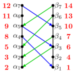
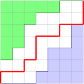
(a)	(b)

Figure 8.1. (a) The Hasse diagram of a poset $P$, and a linear extension $L$ of $P$ (written in red). (b) The corresponding region $\operatorname{\textnormal{Reg}}(P)$, with $F_{\textnormal{up}}(P)$ in green and $F_{\textnormal{down}}(P)$ in blue, and the lattice path $\phi(L)$ in red.

Lemma 8.1.

The map $\phi$ described above is a bijection between  $\operatorname{\mathcal{E}}(P)$  and NE lattice paths in  $\operatorname{\textnormal{Reg}}(P)$  from  $\operatorname{\mathbf{0}}$  to  $(\emph{{a}},\emph{{b}})$.

Proof.

We first show that, for each linear extension $L$, the corresponding lattice path $(Z_{t})_{1\leq t\leq n}$ is contained in  $\operatorname{\textnormal{Reg}}(P)$. Let  $t\in[n]$  and let  $(h,k):=Z_{t}$. Without loss of generality, we assume that $L^{-1}(t)\in\mathcal{C}_{1}$. This implies that $L(\alpha_{h})=t$, which in turn implies that

$$L(\beta_{k})\ <\ L(\alpha_{h})\ <\ L(\beta_{k+1})\hskip 0.85355pt.$$

Now note that  $L(\beta_{k})<L(\alpha_{h})$  implies that  $\beta_{k}\nsucc_{P}\alpha_{h}$, and hence  $\big{(}h-\frac{1}{2},k-\frac{1}{2}\big{)}\notin\operatorname{\textnormal{C}_{\textnormal{up}}}(P)$. By the same reasoning, we have  $\big{(}h-\frac{1}{2},k+\frac{1}{2}\big{)}\notin\operatorname{\textnormal{C}_{\textnormal{down}}}(P)$. This implies that the edge  $\big{[}(h-1,k)\hskip 1.70709pt,\hskip 1.70709pt(h,k)\big{]}\in\operatorname{\textnormal{Reg}}(P)$. Since the choice of $t$ is arbitrary, this implies that the lattice path $(Z_{t})_{1\leq t\leq n}$ is contained in $\operatorname{\textnormal{Reg}}(P)$.

We now construct the inverse map $\phi^{-1}$. Given a lattice path $(Z_{t})_{1\leq t\leq n}$, we construct the corresponding linear extension $L$ as follows. For each $t\in[n]$, let

$$L(\alpha_{h})\ :=\ t\quad\ \text{ if }\ \quad Z_{t}-Z_{t-1}=\textbf{\hskip 0.85355pt{e}${}_{1}$}\ \ \text{ and }\ \ h=Z_{t}(1),$$

$$L(\beta_{k})\ :=\ t\quad\ \text{ if }\ \quad Z_{t}-Z_{t-1}=\textbf{\hskip 0.85355pt{e}${}_{2}$}\ \ \text{ and }\ \ k=Z_{t}(2).$$

It follows from the similar reasoning as above that $L$ respects the poset relations $\prec_{P}$. This completes the proof. ∎

Let  $A=(a_{1},a_{2}),B=(b_{1},b_{2})$  be two integral vertices in $\operatorname{\textnormal{Reg}}(P)$, and let $\zeta$ be a NE lattice path in $\operatorname{\textnormal{Reg}}(P)$ from $A$ to $B$. Define the weight of $\zeta$ by

$$\operatorname{\mathtt{wt}}(\zeta)\ :=\ \text{number of unit boxes in \hskip 0.85355pt$[0,\emph{{a}}]\times[0,\emph{{b}}]$ \hskip 0.85355ptthat lie below $\zeta$}.$$

Recall from (2.6) the definition of the weight function for a linear extension. It is easy to see that $\operatorname{\mathtt{wt}}(\phi(L))\hskip 0.85355pt=\hskip 0.85355pt\operatorname{\mathtt{wt}}(L)-\binom{\emph{{a}}+1}{2}$  for every $L\in\operatorname{\mathcal{E}}(P)$.

8.2. Injective maps between pairs of lattice paths

Let $A,B\in\operatorname{\textnormal{Reg}}(P)$. Denote by  $\mathcal{K}(A,B)$  the set of NE lattice paths $\zeta\in\operatorname{\textnormal{Reg}}(P)$ that starts at $A$ and ends at $B$. Similarly, denote by  $\textrm{K}_{q}(A,B)$  the polynomial

$$\textrm{K}_{q}(A,B)\ :=\ \sum_{\zeta\in\mathcal{K}(A,B)}\hskip 1.70709ptq^{\operatorname{\mathtt{wt}}(\zeta)}\hskip 1.70709pt.$$

Lemma 8.2.

Let  $A,B\in\operatorname{\textnormal{Reg}}(P)$  be on the same vertical line and with $A$ above $B$, i.e.,  $a_{1}=b_{1}$  and  $a_{2}\geq b_{2}$. Let  $C,D\in\operatorname{\textnormal{Reg}}(P)$  be on a vertical line to the right of the line $(AB)$, and with $C$ above $D$.

1. If  $|AB|>|CD|$, i.e.,  $a_{2}-b_{2}>c_{2}-d_{2}$, then

   $$\textrm{\em K}_{q}(A-{\textbf{\hskip 0.85355pt{e}${}_{2}$}},C)\,\cdot\,\textrm{\em K}_{q}(B+{\textbf{\hskip 0.85355pt{e}${}_{2}$}},D)\ \geqslant\ \textrm{\em K}_{q}(A,C)\,\cdot\,\textrm{\em K}_{q}(B,D).$$

2. If  $|CD|>|AB|$, then

   $$\textrm{\em K}_{q}(A,C-{\textbf{\hskip 0.85355pt{e}${}_{2}$}})\,\cdot\,\textrm{\em K}_{q}(B,D+{\textbf{\hskip 0.85355pt{e}${}_{2}$}})\ \geqslant\ \textrm{\em K}_{q}(A,C)\,\cdot\,\textrm{\em K}_{q}(B,D).$$

Informally, the lemma says that there are more pairs of paths closer to the inside than towards the outside of the region. We give a direct combinatorial proof of the lemma by an explicit injection. The injection works by translating the path $B\to D$ upwards so that it starts at $A-\textbf{\hskip 0.85355pt{e}${}_{2}$}$ and ends at $D^{\prime}$. Its translation intersects the path $A\to C$ and by choosing the first intersection point we can swap the paths after the intersection, creating paths $A\to D^{\prime}$ and $A-\textbf{\hskip 0.85355pt{e}${}_{2}$}\to C$. Translating the first path back, we obtain paths $B+\textbf{\hskip 0.85355pt{e}${}_{2}$}\to D$ and $A-\textbf{\hskip 0.85355pt{e}${}_{2}$}\to C$. We show that these paths belong to $\operatorname{\textnormal{Reg}}(P)$, and the map is an injection.

Proof.

We present only the proof of part (a), as the proof of part (b) is analogous. It suffices to show that there exists a weight-preserving injection between two set of pairs of paths

$$\varkappa\,:\ \mathcal{K}(A,C)\hskip 1.70709pt\times\hskip 1.70709pt\mathcal{K}(B,D)\quad\to\quad\mathcal{K}(A-\textbf{\hskip 0.85355pt{e}${}_{2}$},C)\hskip 1.70709pt\times\hskip 1.70709pt\mathcal{K}(B+\textbf{\hskip 0.85355pt{e}${}_{2}$},D).$$

Let  $(\gamma,\zeta)\in\mathcal{K}(A,C)\times\mathcal{K}(B,D)$. We construct a pair  $(\widehat{\gamma},\widehat{\zeta})=\varkappa(\gamma,\zeta)$  as follows.

Figure 8.2. The lattice paths $\gamma$ and $\zeta$ (drawn in blue), the lattice paths $\gamma^{\prime}$ and $\zeta^{\prime}$ (drawn in green), and the lattice paths $\widehat{\gamma}$ and $\widehat{\zeta}$ (drawn in red).

Let $\zeta^{\prime}$ be the path obtained by translating $\zeta$ by  $(0,a_{2}-b_{2}-1)$ , so $\zeta^{\prime}$ starts at  $A^{\prime}=A-\textbf{\hskip 0.85355pt{e}${}_{2}$}$  and ends at  $D^{\prime}=(d_{1},d_{2}+a_{2}-b_{2}-1)$ . Note that $\zeta^{\prime}$ lies above $\zeta$, that $A^{\prime}$ lies below $A$, and that $D^{\prime}$ lies above $C$, by the assumption that  $a_{2}-b_{2}>c_{2}-d_{2}$ . Note also that $\zeta^{\prime}$ does not necessarily belong in $\operatorname{\textnormal{Reg}}(P)$. This implies that paths $\zeta$ and $\zeta^{\prime}$ must intersect, and let $E$ be the first intersection point along these paths.

Let  $\widehat{\gamma}:=\zeta^{\prime}(A^{\prime}\to E)\circ\gamma(E\to C)$  be the NE lattice path $A^{\prime}\to C$, such that $\widehat{\gamma}$ follows the path $\zeta^{\prime}:A^{\prime}\to E$, then follows the path $\gamma:E\to C$. Note that $\widehat{\gamma}\in\operatorname{\textnormal{Reg}}(P)$ since both  $\zeta^{\prime}(A^{\prime}\to E)$  and  $\gamma(E\to C)$  are contained in $\operatorname{\textnormal{Reg}}(P)$. Indeed, the former is due to the minimality of $E$, which implies that this portion of $\zeta^{\prime}$ is below  $\zeta\in\operatorname{\textnormal{Reg}}(P)$.

Similarly, let $\gamma^{\prime}$ be the path obtained by translating  $\gamma$  by  $(0,-a_{2}+b_{2}+1)$. Note that $\gamma^{\prime}$ starts at $B^{\prime}=B+\textbf{\hskip 0.85355pt{e}${}_{2}$}$, and that the first intersection point between $\gamma^{\prime}$ and $\zeta$ is  $E^{\prime}:=E+(0,-a_{2}+b_{2}+1)$. Let  $\widehat{\zeta}:=\gamma^{\prime}(B^{\prime}\to E^{\prime})\circ\zeta(E^{\prime}\to D)$  be the NE lattice path $B^{\prime}\to D$, such that  $\widehat{\zeta}$  follows the path $\gamma^{\prime}:B^{\prime}\to E^{\prime}$, then follows the path $\zeta:E^{\prime}\to D$. Note that  $\widehat{\zeta}\in\operatorname{\textnormal{Reg}}(P)$, since  $\gamma^{\prime}(B^{\prime}\to E^{\prime}),\hskip 1.70709pt\zeta(E^{\prime}\to D)\in\operatorname{\textnormal{Reg}}(P)$.

It follows from the construction above that  $(\gamma^{\prime},\zeta^{\prime})\in\mathcal{K}(A-\textbf{\hskip 0.85355pt{e}${}_{2}$},C)\times\mathcal{K}(B+\textbf{\hskip 0.85355pt{e}${}_{2}$},D)$. This map is injective as $\gamma$ and $\zeta$ can be recovered uniquely by identifying the first intersection point $E$. Furthermore, this is a weight-preserving map, since

(8.1) $$\operatorname{\mathtt{wt}}(\gamma)\hskip 1.70709pt+\hskip 1.70709pt\operatorname{\mathtt{wt}}(\zeta) =\ \operatorname{\mathtt{wt}}\big{(}\gamma(A\to E)\big{)}\hskip 1.70709pt+\hskip 1.70709pt\operatorname{\mathtt{wt}}\big{(}\gamma(E\to C)\big{)}\hskip 1.70709pt+\hskip 1.70709pt\operatorname{\mathtt{wt}}\big{(}\zeta(B\to E^{\prime})\big{)}\hskip 1.70709pt+\hskip 1.70709pt\operatorname{\mathtt{wt}}\big{(}\zeta(E^{\prime}\to D)\big{)}$$

$$=\ \operatorname{\mathtt{wt}}\big{(}\gamma^{\prime}(B^{\prime}\to E^{\prime})\big{)}\hskip 1.70709pt+\hskip 1.70709pt(e_{1}-a_{1})\times(a_{2}+b_{2}-1)\hskip 1.70709pt+\hskip 1.70709pt\operatorname{\mathtt{wt}}\big{(}\gamma(E\to C)\big{)}$$

$$\hskip 45.52458pt+\,\operatorname{\mathtt{wt}}\big{(}\zeta^{\prime}(A^{\prime}\to E)\big{)}\hskip 1.70709pt-\hskip 1.70709pt(e_{1}-a_{1})\times(a_{2}+b_{2}-1)\hskip 1.70709pt+\hskip 1.70709pt\operatorname{\mathtt{wt}}\big{(}\zeta(E^{\prime}\to D)\big{)}$$

$$=\ \operatorname{\mathtt{wt}}\big{(}\zeta^{\prime}(A^{\prime}\to E)\big{)}\hskip 1.70709pt+\hskip 1.70709pt\operatorname{\mathtt{wt}}\big{(}\gamma(E\to C)\big{)}\hskip 1.70709pt+\hskip 1.70709pt\operatorname{\mathtt{wt}}\big{(}\gamma^{\prime}(B^{\prime}\to E^{\prime})\big{)}\hskip 1.70709pt+\hskip 1.70709pt\operatorname{\mathtt{wt}}\big{(}\zeta(E^{\prime}\to D)\big{)}$$

$$=\ \operatorname{\mathtt{wt}}(\widehat{\gamma})\hskip 1.70709pt+\hskip 1.70709pt\operatorname{\mathtt{wt}}(\widehat{\zeta})\hskip 1.70709pt.$$

This completes the proof. ∎

Remark 8.3.

The equation (8.1) may seem remarkably coincidental, but can be easily explained. Note that when we switch paths at intersections, the areas below paths can change but the sum of areas remain the same via  $|U|+|V|=|U\cap V|+|U\cap V|$  for all finite sets  $U,V$  of lattice squares.

Lemma 8.4.

Let  $A,B,C,D\in\operatorname{\textnormal{Reg}}(P)$  be as in Lemma 8.2. We then have the following conditions for equalities in Lemma 8.2:

1. If  $|AB|>|CD|$, i.e.,  $a_{2}-b_{2}>c_{2}-d_{2}$, then

   $$\textrm{\em K}(A-{\textbf{\hskip 0.85355pt{e}${}_{2}$}},C)\,\cdot\,\textrm{\em K}(B+{\textbf{\hskip 0.85355pt{e}${}_{2}$}},D)\ =\ \textrm{\em K}(A,C)\,\cdot\,\textrm{\em K}(B,D)$$

   if and only if both sides are zero, or

   $$\textrm{\em K}(A-{\textbf{\hskip 0.85355pt{e}${}_{2}$}},C)\ =\ \textrm{\em K}(A,C)\qquad\text{and}\qquad\textrm{\em K}(B+{\textbf{\hskip 0.85355pt{e}${}_{2}$}},D)\ =\ \textrm{\em K}(B,D)\ =\ \textrm{\em K}(A,D).$$

2. If  $|CD|>|AB|$, then

   $$\textrm{\em K}(A,C-{\textbf{\hskip 0.85355pt{e}${}_{2}$}})\,\cdot\,\textrm{\em K}(B,D+{\textbf{\hskip 0.85355pt{e}${}_{2}$}})\ =\ \textrm{\em K}(A,C)\,\cdot\,\textrm{\em K}(B,D)$$

   if and only if both sides are zero, or

   $$\textrm{\em K}(A,C-{\textbf{\hskip 0.85355pt{e}${}_{2}$}})\ =\ \textrm{\em K}(A,C)\ =\ \textrm{\em K}(A,D)\qquad\text{and}\qquad\textrm{\em K}(B,D+{\textbf{\hskip 0.85355pt{e}${}_{2}$}})\ =\ \textrm{\em K}(B,D).$$

In both cases, the equality of the number of paths implies the corresponding path collections coincide, so the $q$-weights are also preserved.

This lemma analyzes when equality in Lemma 8.2 occurs, which is equivalent to the lattice path involution $\varkappa$ being a bijection. We show that unless all these paths pass vertically through points $A$ and $B$, see Figure 8.3, there will always be an “extreme” pair of paths not contained in the image of $\varkappa$.

Figure 8.3. The proof of the equality case, Lemma 8.4. The green path $\eta$ is the lowest in $\operatorname{\textnormal{Reg}}(P)$ from $A^{\prime}\to C$, and the blue path $\xi$ is the highest in the region from $B^{\prime}\to D$. The cyan $\xi^{\prime}=\xi+v$ is the vertical translation of $\xi$, which intersects $\eta$ at point $E$ (first such intersection). The inverse paths $\varkappa^{-1}(\eta,\xi)=(\widehat{\eta},\widehat{\xi})$ are drawn on top in red and brown.

Proof.

We prove only part (a), as part (b) follows analogously. Clearly, the “if” direction follows immediately.

For the “only if” direction, assume that the products are equal. We will show that  $\textrm{\em K}(A-{\textbf{\hskip 0.85355pt{e}${}_{2}$}},C)\,=\,\textrm{\em K}(A,C)$  and  $\textrm{\em K}(B+{\textbf{\hskip 0.85355pt{e}${}_{2}$}},D)\,=\,\textrm{\em K}(B,D)$. From the proof of Lemma 8.2, the equality implies that the injection $\varkappa$ is a bijection, and hence surjective.

Let $\hskip 1.70709pt\eta:A^{\prime}=A-\textbf{\hskip 0.85355pt{e}${}_{2}$}\to C$  be the lowest possible path within  $\operatorname{\textnormal{Reg}}(P)$  between these two points, and similarly  $\xi:B^{\prime}=B+\textbf{\hskip 0.85355pt{e}${}_{2}$}\to D$  be the highest possible path within  $\operatorname{\textnormal{Reg}}(P)$  between the given points, see Figure 8.3. Let  $\xi^{\prime}:A\to D^{\prime}$  (which passes above the point $C$) be the vertical translation of $\xi$. Since $\varkappa$ is a bijection, we must have that $\eta$ and $\xi^{\prime}$ intersect and their preimages belong to  $\operatorname{\textnormal{Reg}}(P)$.

First, if $d_{2}\leq a^{\prime}_{2}$, then the paths are $\xi=B^{\prime}\to(b_{1}^{\prime},d_{2})\to D$ and $\eta:A^{\prime}\to(c_{1},a_{2}^{\prime})\to C$. Thus $\xi^{\prime}$ lies strictly above $\eta$. Therefore, these paths do not intersect, and hence  $d_{2}>a_{2}^{\prime}$. Since $A^{\prime}\in\operatorname{\textnormal{Reg}}(P)$, $A^{\prime}$ is lower than $D$ and $\xi$ is the highest path from $B^{\prime}$ to $D$, so we must have that $\xi=B^{\prime}\to A^{\prime}\to D$. Similarly, the lowest path must pass through $D$, so $\eta:A^{\prime}\to D\to C$. Furthermore, the path $\eta(A^{\prime}\to D)$ is weakly below the path $\xi(A^{\prime}\to D)$. Let $v=(0,a_{2}-b_{2}-1)$, the translation vector.

Since there exists a preimage  $\varkappa^{-1}(\eta,\xi)$, this implies that paths  $\xi^{\prime}$ and $\eta$  intersect. Let $E$ be the first intersection of  $\xi^{\prime}$ and $\eta$. Since  $\eta(A^{\prime}\to D)$  is weakly below paths  $\xi$ and $\xi+v$, the point $E$ must belong to all three paths. Then

$$\varkappa^{-1}\bigl{(}\eta,\xi\bigr{)}\,=\,\bigl{(}\hskip 0.85355pt\widehat{\eta},\hskip 0.85355pt\widehat{\xi}\hskip 1.70709pt\bigr{)}\hskip 0.85355pt,$$

where  $\widehat{\eta}=(\xi(B^{\prime}\to E^{\prime})+v)\circ\eta(E\to C)$  is a path from  $A$ to $C$, and  $\widehat{\xi}=(\eta(A^{\prime}\to E)-v)\circ\xi(E^{\prime}\to D)$  is a path from  $B\to D$. Now note that through our assumption of $\varkappa$ being a bijection, we must have that $\widehat{\eta}$ and $\widehat{\xi}$ are both in $\operatorname{\textnormal{Reg}}(P)$. Note that $\widehat{\eta}$ begins with the translation of $\xi$ by $v$, and the point  $E\in\eta(A^{\prime}\to D)\subset\operatorname{\textnormal{Reg}}(P)$. Hence  $(B^{\prime}\to A)\circ\widehat{\eta}(A\to E)\circ\xi(E\to D)\in\operatorname{\textnormal{Reg}}(P)$  is a path which is higher than $\xi$ in $\operatorname{\textnormal{Reg}}(P)$. This causes a contradiction except in the case when $E$ is on the line through $A^{\prime}B^{\prime}$ (and has to be equal to $A$). This means that the lowest path  $\eta:A^{\prime}\to C$  starts with a vertical step, i.e. $A^{\prime}+\textbf{\hskip 0.85355pt{e}${}_{1}$}\not\in\operatorname{\textnormal{Reg}}(P)$, and hence the lower border of  $\operatorname{\textnormal{Reg}}(P)$  contains the segment $(B,A)$. This implies that, every path in $\operatorname{\textnormal{Reg}}(P)$ that passes through a point in  $\{B,B^{\prime},A^{\prime}\}$  must also pass through $A$.

We conclude that  $\textrm{K}(A,C)=\textrm{K}(A^{\prime},C)$, and every path  $A^{\prime}\to C$ in $\operatorname{\textnormal{Reg}}(P)$ passes through $A$. Similarly, we have  $\textrm{K}(B,D)=\textrm{K}(B^{\prime},D)=\textrm{K}(A,D)$. Finally, for the $q$-analogues we also have  $\textrm{K}_{q}(A,C)=\textrm{K}_{q}(A^{\prime},C)$  and  $\textrm{K}_{q}(B,D)=\textrm{K}_{q}(B^{\prime},D)$, since the weights are preserved under $\varkappa$. ∎

Lemma 8.5.

Let   $A,B\in\operatorname{\textnormal{Reg}}(P)$  be in the same horizontal line and with $A$ to the left of $B$, i.e.  $a_{2}=b_{2}$  and  $a_{1}\leq b_{1}$. Let $C,D\in\operatorname{\textnormal{Reg}}(P)$ be in a vertical line that is above the line  $(AB)$, i.e.  $c_{2},d_{2}\geq a_{2}$, and with $C$ below $D$.

1. If  $|AB|>0$, i.e.  $b_{1}-a_{1}>0$, then:

   $$\textrm{\em K}_{q}(A+{\textbf{\hskip 0.85355pt{e}${}_{1}$}},C)\,\cdot\,\textrm{\em K}_{q}(B-{\textbf{\hskip 0.85355pt{e}${}_{1}$}},D)\ \geqslant\ \textrm{\em K}_{q}(A,C)\,\cdot\,\textrm{\em K}_{q}(B,D).$$

2. If  $|CD|>0$, then:

   $$\textrm{\em K}_{q}(A,C+{\textbf{\hskip 0.85355pt{e}${}_{2}$}})\,\cdot\,\textrm{\em K}_{q}(B,D-{\textbf{\hskip 0.85355pt{e}${}_{2}$}})\ \geqslant\ \textrm{\em K}_{q}(A,C)\,\cdot\,\textrm{\em K}_{q}(B,D).$$

Proof.

We present only the proof of part (a), as the proof of part (b) is analogous. It suffices to show that there exists a weight-preserving injection between two set of pairs of paths

$$\varkappa\,:\,\mathcal{K}(A,C)\hskip 1.70709pt\times\hskip 1.70709pt\mathcal{K}(B,D)\ \to\ \mathcal{K}(A+\textbf{\hskip 0.85355pt{e}${}_{1}$},C)\hskip 1.70709pt\times\hskip 1.70709pt\mathcal{K}(B-\textbf{\hskip 0.85355pt{e}${}_{1}$},D).$$

Let  $(\gamma,\zeta)\in\mathcal{K}(A,C)\hskip 0.85355pt\times\hskip 0.85355pt\mathcal{K}(B,D)$. We construct a pair  $(\widehat{\gamma},\widehat{\zeta})=\varkappa(\gamma,\zeta)$  as follows.

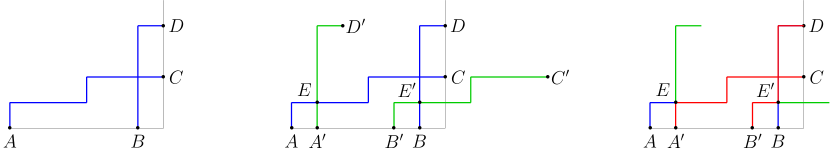
Figure 8.4. The lattice paths $\gamma$ and $\zeta$ (drawn in blue), the lattice paths $\gamma^{\prime}$ and $\zeta^{\prime}$ (drawn in green), and the lattice paths $\widehat{\gamma}$ and $\widehat{\zeta}$ (drawn in red).

Let $\zeta^{\prime}$ be the path obtained by translating $\zeta$ by  $(a_{1}-b_{1}+1,0)$ , so $\zeta^{\prime}$ starts at  $A^{\prime}=A+(1,0)$  and ends at  $D^{\prime}=(d_{1}+a_{1}-b_{1}+1,d_{2})$ . Note that $\zeta^{\prime}$ lies to the left of $\zeta$, that $A^{\prime}$ lies to right of $A$, and that $D^{\prime}$ lies to the left of $D$, by the assumption that  $b_{1}-a_{1}>0$ . This implies that the path $\zeta$ and $\zeta^{\prime}$ must intersect, and let $E$ be the first intersection point along these paths. Let  $\widehat{\gamma}:=\zeta^{\prime}(A^{\prime}\to E)\circ\gamma(E\to C)$  be the NE lattice path from  $A^{\prime}\to C$, such that  $\widehat{\gamma}$  follows the path  $\zeta^{\prime}:A^{\prime}\to E$, then follows the path  $\gamma:E\to C$.

Let $\gamma^{\prime}$ be the path obtained by translating $\gamma$ by  $(-a_{2}+b_{2}-1,0)$ . Note that $\gamma^{\prime}$ starts at $B^{\prime}=B-(1,0)$, and that the first intersection point between $\gamma^{\prime}$ and $\zeta$ is  $E^{\prime}:=E+(-a_{2}+b_{2}-1,0)$ . Let  $\widehat{\zeta}:=\gamma^{\prime}(B^{\prime}\to E^{\prime})\hskip 1.70709pt\zeta(E^{\prime},D)$  be the NE lattice path from $B^{\prime}$ to $D$, such that  $\widehat{\zeta}$  follows the path  $\gamma^{\prime}:B^{\prime}\to E^{\prime}$, then follows the path  $\zeta:E^{\prime}\to D$.

It follows from the same argument as in the proof of Lemma 8.2, that $\varkappa$ is an injective, weight-preserving map from  $\mathcal{K}(A,C)\hskip 1.70709pt\times\hskip 1.70709pt\mathcal{K}(B,D)$  to  $\mathcal{K}(A+\textbf{\hskip 0.85355pt{e}${}_{1}$},C)\hskip 1.70709pt\times\hskip 1.70709pt\mathcal{K}(B-\textbf{\hskip 0.85355pt{e}${}_{1}$},D)$. This completes the proof. ∎

9. Lattice paths proof of Theorem 1.7

9.1. Setting up the injection

We should mention that to simplify the notation, from this point on we will use  $z_{1}\leftarrow x$,  $z_{2}\leftarrow y$, and  $z_{3}\leftarrow z$, and also $i\leftarrow k$, $j\leftarrow\ell$ in Theorem 1.7. By relabeling $\mathcal{C}_{1}$ and $\mathcal{C}_{2}$ and substituting $q$ with $q^{-1}$ if necessary, we will without loss of generality assume that  $z_{2}\in\mathcal{C}_{1}$.

The idea is to consider the lattice paths in $\operatorname{\textnormal{Reg}}(P)$ based on the position of the horizontal step above $z_{2}$, which also corresponds to the value of $L(z_{2})$. The summands in $\textrm{F}_{q}(i,j)$ correspond to lattice paths, which can be grouped according to their horizontal steps above $z_{2}$, say $Y\to Y+\textbf{\hskip 0.85355pt{e}${}_{1}$}$. The $i$ and $j$ give the grid distance to $Y$ from this step to the horizontal (when all $z$s are in $\mathcal{C}_{1}$) step above $z_{1}$ and $z_{3}$ respectively, see Figure 9.2. We can expand the difference

$$\textrm{F}_{q}(i,j)\ \textrm{F}_{q}(i+1,j+1)\ -\ \textrm{F}_{q}(i+1,j)\ \textrm{F}_{q}(i,j+1)$$

as sums of pairs of lattice paths passing through the same two points above $z_{2}$. Then $i,i+1$ and $j,j+1$ determine which paths pass closer to each other, and we can derive the inequality by multiple applications of Lemmas 8.2 and 8.5 depending on which chains $z_{1},z_{3}$ belong to.

Let $i,j\geq 1$ and let $Y\in\operatorname{\textnormal{Reg}}(P)$. We denote by $\operatorname{\mathcal{G}}(i,Y)$ the set of NE lattice paths  $\operatorname{\mathbf{0}}\to Y$ in $\operatorname{\textnormal{Reg}}(P)$  that pass through  $Y-I$  and  $Y-I+U_{1}$ , where  $I=I(i,Y)$  and  $U_{1}$  are defined as

$$I\ :=\ \begin{cases}(y_{1}-k+1,i-y_{1}+k-1)\ \ &\text{ if \ \, $z_{1}\in\mathcal{C}_{1}$\hskip 0.85355pt, \, and \, $z_{1}=\alpha_{k}$\hskip 1.70709pt,}\\ (i-y_{2}+k-1,y_{2}-k+1)\ \ &\text{ if \ \, $z_{1}\in\mathcal{C}_{2}$\hskip 0.85355pt, \, and \, $z_{1}=\beta_{k}$\hskip 1.70709pt.}\end{cases}$$

$$U_{1}\ :=\ \begin{cases}\textbf{\hskip 0.85355pt{e}${}_{1}$}&\ \,\text{ if }\ \,z_{1}\in\mathcal{C}_{1}\hskip 1.70709pt,\\ \textbf{\hskip 0.85355pt{e}${}_{2}$}&\ \,\text{ if }\ \,z_{1}\in\mathcal{C}_{2}\hskip 1.70709pt.\end{cases}$$

Similarly, denote by $\operatorname{\mathcal{H}}(j,Y)$ the set of NE lattice paths  $Y+\textbf{\hskip 0.85355pt{e}${}_{1}$}\to(\emph{{a}},\emph{{b}})$  in $\operatorname{\textnormal{Reg}}(P)$ that pass through  $Y+J$  and  $Y+J+U_{3}$ , where  $J=J(j,Y)$  and  $U_{3}$  are defined as

$$J\ :=\ \begin{cases}(m-y_{1}-1,j+y_{1}-m+1)\ \ &\text{ if \ \, $z_{3}\in\mathcal{C}_{1}$\hskip 0.85355pt, \, and \, $z_{3}\hskip 1.70709pt=:\hskip 1.70709pt\alpha_{m}$\hskip 1.70709pt,}\\ (j+y_{2}-m+1,m-y_{2}-1)\ \ &\text{ if \ \, $z_{3}\in\mathcal{C}_{2}$\hskip 0.85355pt, \, and \, $z_{3}\hskip 1.70709pt=:\hskip 1.70709pt\beta_{m}$\hskip 1.70709pt.}\\ \end{cases}$$

$$U_{3}\ :=\ \begin{cases}\textbf{\hskip 0.85355pt{e}${}_{1}$}&\ \,\text{ if }\ \,z_{3}\in\mathcal{C}_{1}\hskip 1.70709pt,\\ \textbf{\hskip 0.85355pt{e}${}_{2}$}&\ \,\text{ if }\ \,z_{3}\in\mathcal{C}_{2}\hskip 1.70709pt.\end{cases}$$

Finally, denote

$$\textrm{G}_{q}(i,Y)\ :=\ \sum_{\gamma\in\operatorname{\mathcal{G}}(i,Y)}\hskip 1.70709ptq^{\operatorname{\mathtt{wt}}(\gamma)}\qquad\text{and}\qquad\textrm{H}_{q}(j,Y)\ :=\ \sum_{\gamma\in\operatorname{\mathcal{H}}(j,Y)}\hskip 1.70709ptq^{\operatorname{\mathtt{wt}}(\gamma)}\hskip 1.70709pt.$$

Recall the map $\phi$ defined in the previous section. Each linear extension $L\in\operatorname{\mathcal{E}}(P)$ such that

$$L(z_{2})=u,\quad L(z_{2})-L(z_{1})=i\quad\text{and}\quad L(z_{3})-L(z_{2})=j,$$

corresponds to a NE lattice path  $(0,0)\to(\emph{{a}},\emph{{b}})$ in $\operatorname{\textnormal{Reg}}(P)$ that passes through

$${Y^{\langle u\rangle}}-I,\quad{Y^{\langle u\rangle}}-I+U_{1},\quad{Y^{\langle u\rangle}},\quad{Y^{\langle u\rangle}}+\textbf{\hskip 0.85355pt{e}${}_{1}$},\quad{Y^{\langle u\rangle}}+J,\quad{Y^{\langle u\rangle}}+J+U_{3}\hskip 1.70709pt,$$

where  ${Y^{\langle u\rangle}}\hskip 1.70709pt:=\hskip 1.70709pt(\ell-1,u-\ell)$ , and $\ell$ is the integer such that  $z_{2}=\alpha_{\ell}$. That is, such a linear extension corresponds to a lattice path where the first half is contained in  $\operatorname{\mathcal{G}}\bigl{(}i,{Y^{\langle u\rangle}}\bigr{)}$  and the second half is contained in  $\operatorname{\mathcal{H}}\bigl{(}j,{Y^{\langle u\rangle}}\bigr{)}$ . See Figure 9.1 for an example.

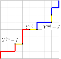
Figure 9.1. A lattice path that corresponds to a linear extension in $\operatorname{\mathcal{F}}(i,j)$, with $i=j=4$ and $L(z_{2})=u=8$. Note that $z_{1},z_{2}\in\mathcal{C}_{1}$ and $z_{3}\in\mathcal{C}_{2}$. The first half of the lattice path $(0,0)\to(4,4)$ (in red) is contained in  $\operatorname{\mathcal{G}}\bigl{(}i,{Y^{\langle u\rangle}}\bigr{)}$, and the second half of the path $(5,4)\to(8,8)$ (in blue) is contained in  $\operatorname{\mathcal{H}}\bigl{(}j,{Y^{\langle u\rangle}}\bigr{)}$.

It now follows from the correspondence above that

$$\textrm{F}_{q}(i,j)\ =\ q^{\binom{\emph{{a}}+1}{2}}\,\sum_{u=1}^{n}\,q^{u-\ell}\hskip 1.70709pt\textrm{G}_{q}\bigl{(}i,{Y^{\langle u\rangle}}\bigr{)}\,\textrm{H}_{q}\bigl{(}j,{Y^{\langle u\rangle}}\bigr{)}\hskip 0.85355pt.$$

Applying the formula above to the polynomials  $\textrm{F}_{q}(i,j)\hskip 1.70709pt\textrm{F}_{q}(i+1,j+1)$ and  $\textrm{F}_{q}(i+1,j)\hskip 1.70709pt\textrm{F}_{q}(i,j+1)$ , we get

$$\begin{split}&\textrm{F}_{q}(i,j)\,\textrm{F}_{q}(i+1,j+1)\ =\ q^{\emph{{a}}(\emph{{a}}+1)}\,\sum_{u=1}^{n}\,\sum_{w=1}^{n}\,q^{u+w-2\ell}\hskip 1.70709pt\textrm{G}_{q}\bigl{(}i,{Y^{\langle u\rangle}}\bigr{)}\hskip 1.70709pt\textrm{H}_{q}\bigl{(}j,{Y^{\langle u\rangle}}\bigr{)}\ \textrm{G}_{q}\big{(}i+1,{Y^{\langle w\rangle}}\big{)}\ \textrm{H}_{q}(j+1,{Y^{\langle w\rangle}}),\\ &\textrm{F}_{q}(i+1,j)\hskip 1.70709pt\textrm{F}_{q}(i,j+1)\ =\ q^{\emph{{a}}(\emph{{a}}+1)}\,\sum_{u=1}^{n}\hskip 1.70709pt\sum_{w=1}^{n}\,q^{u+w-2\ell}\hskip 1.70709pt\textrm{G}_{q}\big{(}i+1,{Y^{\langle u\rangle}}\big{)}\hskip 1.70709pt\textrm{H}_{q}(j,{Y^{\langle u\rangle}})\ \textrm{G}_{q}\big{(}i,{Y^{\langle w\rangle}}\big{)}\ \textrm{H}_{q}\big{(}j+1,{Y^{\langle w\rangle}}\big{)}.\end{split}$$

Taking the difference between the two equation above, we get

(9.1) $$\begin{split}&\textrm{F}_{q}(i,j)\hskip 1.70709pt\textrm{F}_{q}(i+1,j+1)\hskip 1.70709pt-\hskip 1.70709pt\textrm{F}_{q}(i+1,j)\hskip 1.70709pt\textrm{F}_{q}(i,j+1)\\ &\hskip 28.45274pt=\ q^{\emph{{a}}(\emph{{a}}+1)}\,\sum_{u=1}^{n}\hskip 1.70709pt\sum_{w=1}^{n}\,q^{u+w-2\ell}\hskip 1.70709pt\textrm{H}_{q}\big{(}j,{Y^{\langle u\rangle}}\big{)}\ \textrm{H}_{q}\big{(}j+1,{Y^{\langle w\rangle}}\big{)}\ \times\\ &\hskip 85.35826pt\times\ \bigl{[}\textrm{G}_{q}\big{(}i,{Y^{\langle u\rangle}}\big{)}\ \textrm{G}_{q}\big{(}i+1,{Y^{\langle w\rangle}}\big{)}\ -\ \textrm{G}_{q}\big{(}i+1,{Y^{\langle u\rangle}}\big{)}\ \textrm{G}_{q}\big{(}i,{Y^{\langle w\rangle}}\big{)}\bigr{]}\\ &\hskip 28.45274pt=\ q^{\emph{{a}}(\emph{{a}}+1)}\,\sum_{1\leq u<w\leq n}\,q^{u+w-2\ell}\,\operatorname{\textnormal{GCP}}_{q}\big{(}i,{Y^{\langle u\rangle}},{Y^{\langle w\rangle}}\big{)}\,\operatorname{\textnormal{HCP}}_{q}\big{(}j,{Y^{\langle u\rangle}},{Y^{\langle w\rangle}}\big{)}\hskip 1.70709pt,\end{split}$$

where

$$\operatorname{\textnormal{GCP}}_{q}(i,Y,V)\ :=\ \textrm{G}_{q}(i,Y)\ \textrm{G}_{q}(i+1,V)\ -\ \textrm{G}_{q}(i+1,Y)\ \textrm{G}_{q}(i,V),$$

$$\operatorname{\textnormal{HCP}}_{q}(j,Y,V)\ :=\ \textrm{H}_{q}(j,Y)\ \textrm{H}_{q}(j+1,V)\ -\ \textrm{H}_{q}(j+1,Y)\ \textrm{H}_{q}(j,V).$$

Now observe that the theorem is reduced to the following result:

Lemma 9.1.

Let $Y,V\in\operatorname{\textnormal{Reg}}(P)$ be in the same vertical line and with $Y$ below $V$. Then

$$\operatorname{\textnormal{GCP}}_{q}(i,Y,V)\ \geqslant\ 0\qquad\text{ and }\qquad\operatorname{\textnormal{HCP}}_{q}(j,Y,V)\ \leqslant\ 0\hskip 1.70709pt.$$

Proof of Theorem 1.7.

To obtain the theorem, apply the lemma to all the terms in (9.1). This gives

$$\textrm{F}_{q}(i,j)\,\hskip 1.70709pt\textrm{F}_{q}(i+1,j+1)\ \geqslant\ \textrm{F}_{q}(i+1,j)\,\hskip 1.70709pt\textrm{F}_{q}(i,j+1)\hskip 0.85355pt,$$

as desired. ∎

9.2. Proof of Lemma 9.1

We prove only the inequality  $\operatorname{\textnormal{GCP}}_{q}(i,Y,V)\hskip 1.70709pt\geq\hskip 1.70709pt0$ as the proof of the other inequality is analogous.

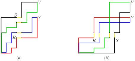
Figure 9.2. Two instances of lattice paths in $\operatorname{\mathcal{G}}(i,Y)$ (in blue), $\operatorname{\mathcal{G}}(i,V)$ (in black), $\operatorname{\mathcal{G}}(i+1,Y)$ (in red), and $\operatorname{\mathcal{G}}(i+1,V)$ (in green). Note that $z_{1}\in\mathcal{C}_{1}$ and $i=7$ in part (a), while $z_{1}\in\mathcal{C}_{2}$ and $i=10$ in part (b).

We split the proof into two cases. For the first case, suppose that $z_{1}\in\mathcal{C}_{1}$. Let

$$R\ :=\ Y\hskip 1.70709pt-\hskip 1.70709ptI(i+1,Y)\,=\,(r_{1},r_{2}),\qquad S\ :=\ V\hskip 1.70709pt-\hskip 1.70709ptI(i,V)\,=\,(s_{1},s_{2})\hskip 0.85355pt.$$

These are the points above $z_{1}$ where the lattice paths pass through. In particular, the lattice paths in  $\operatorname{\mathcal{G}}(i,Y)$  start at  $\operatorname{\mathbf{0}}$, ends at $Y$, and passes through  $R+\textbf{\hskip 0.85355pt{e}${}_{2}$}$  and  $R\hskip 0.85355pt+\hskip 0.85355pt\textbf{\hskip 0.85355pt{e}${}_{1}$}\hskip 0.85355pt+\hskip 0.85355pt\textbf{\hskip 0.85355pt{e}${}_{2}$}$. It then follows that

(9.2) $$\textrm{G}_{q}(i,Y)\ =\ \textrm{K}_{q}(\operatorname{\mathbf{0}},R+\textbf{\hskip 0.85355pt{e}${}_{2}$})\ q^{r_{2}+1}\ \textrm{K}_{q}(R+\textbf{\hskip 0.85355pt{e}${}_{1}$}+\textbf{\hskip 0.85355pt{e}${}_{2}$},Y)\hskip 1.70709pt.$$

By an analogous reasoning, we have

(9.3) $$\begin{split}\textrm{G}_{q}(i+1,Y)\ &=\ \textrm{K}_{q}(\operatorname{\mathbf{0}},R)\ q^{r_{2}}\,\textrm{K}_{q}(R+\textbf{\hskip 0.85355pt{e}${}_{1}$},Y)\hskip 0.85355pt,\\ \textrm{G}_{q}(i,V)\ &=\ \textrm{K}_{q}(\operatorname{\mathbf{0}},S)\ q^{s_{2}}\,\textrm{K}_{q}(S+\textbf{\hskip 0.85355pt{e}${}_{1}$},V)\hskip 0.85355pt,\\ \textrm{G}_{q}(i+1,V)\ &=\ \textrm{K}_{q}(\operatorname{\mathbf{0}},S-\textbf{\hskip 0.85355pt{e}${}_{2}$})\ q^{s_{2}-1}\,\textrm{K}_{q}(S+\textbf{\hskip 0.85355pt{e}${}_{1}$}-\textbf{\hskip 0.85355pt{e}${}_{2}$},V)\hskip 0.85355pt.\end{split}$$

It then follows from (9.2) and (9.3) that

$$\textrm{G}_{q}(i,Y)\,\textrm{G}_{q}(i+1,V)\ =\ q^{r_{2}+s_{2}}\,\bigg{(}\textrm{K}_{q}(\operatorname{\mathbf{0}},S-\textbf{\hskip 0.85355pt{e}${}_{2}$})\,\textrm{K}_{q}(\operatorname{\mathbf{0}},R+\textbf{\hskip 0.85355pt{e}${}_{2}$})\bigg{)}\,\bigg{(}\textrm{K}_{q}(S+\textbf{\hskip 0.85355pt{e}${}_{1}$}-\textbf{\hskip 0.85355pt{e}${}_{2}$},V)\,\textrm{K}_{q}(R+\textbf{\hskip 0.85355pt{e}${}_{1}$}+\textbf{\hskip 0.85355pt{e}${}_{2}$},Y)\bigg{)}.$$

We now apply Lemma 8.2 (a) to the last product term  $\textrm{K}_{q}(S+\textbf{\hskip 0.85355pt{e}${}_{1}$}-\textbf{\hskip 0.85355pt{e}${}_{2}$},V)\hskip 1.70709pt\textrm{K}_{q}(R+\textbf{\hskip 0.85355pt{e}${}_{1}$}+\textbf{\hskip 0.85355pt{e}${}_{2}$},Y)$  in the equation above, with  $A=S+\textbf{\hskip 0.85355pt{e}${}_{1}$}$ ,  $B=R+\textbf{\hskip 0.85355pt{e}${}_{1}$}$ ,  $C=V$  and  $D=Y$. We get:

$$\textrm{G}_{q}(i,Y)\ \textrm{G}_{q}(i+1,V)\ \geqslant\ q^{r_{2}+s_{2}}\ \bigg{(}\textrm{K}_{q}(\operatorname{\mathbf{0}},S-\textbf{\hskip 0.85355pt{e}${}_{2}$})\ \textrm{K}_{q}(\operatorname{\mathbf{0}},R+\textbf{\hskip 0.85355pt{e}${}_{2}$})\bigg{)}\,\bigg{(}\textrm{K}_{q}(S+\textbf{\hskip 0.85355pt{e}${}_{1}$},V)\ \textrm{K}_{q}(R+\textbf{\hskip 0.85355pt{e}${}_{1}$},Y)\bigg{)}.$$

We now apply Lemma 8.2 (b) to first product term  $\textrm{K}_{q}(\operatorname{\mathbf{0}},S-\textbf{\hskip 0.85355pt{e}${}_{2}$})\hskip 1.70709pt\textrm{K}_{q}(\operatorname{\mathbf{0}},R+\textbf{\hskip 0.85355pt{e}${}_{2}$})$  in the equation above. We get: with  $A=B=\operatorname{\mathbf{0}}$ ,  $C=S$  and  $D=R$,

$$\textrm{G}_{q}(i,Y)\ \textrm{G}_{q}(i+1,V)\ \geqslant\ q^{r_{2}+s_{2}}\ \bigg{(}\textrm{K}_{q}(\operatorname{\mathbf{0}},S)\ \textrm{K}_{q}(\operatorname{\mathbf{0}},R)\bigg{)}\,\bigg{(}\textrm{K}_{q}(S+\textbf{\hskip 0.85355pt{e}${}_{1}$},V)\ \textrm{K}_{q}(R+\textbf{\hskip 0.85355pt{e}${}_{1}$},Y)\bigg{)}.$$

It then follows from (9.3) that

$$\textrm{G}_{q}(i,Y)\ \textrm{G}_{q}(i+1,V)\ \geqslant\ \textrm{G}_{q}(i+1,Y)\ \textrm{G}_{q}(i,V)\hskip 0.85355pt.$$

This proves that  $\operatorname{\textnormal{GCP}}_{q}(i,Y,V)\hskip 1.70709pt\geqslant\hskip 1.70709pt0$  for the first case.

For the second case, suppose that $z_{1}\in\mathcal{C}_{2}$. We write

$$R\ :=\ Y\hskip 1.70709pt-\hskip 1.70709ptI(i,Y),\qquad S\ :=\ V\hskip 1.70709pt-\hskip 1.70709ptI(i+1,V)\hskip 1.70709pt.$$

It then follows that

(9.4) $$\begin{split}\textrm{G}_{q}(i,Y)\ &=\ \textrm{K}_{q}(\operatorname{\mathbf{0}},R+\textbf{\hskip 0.85355pt{e}${}_{1}$})\ \textrm{K}_{q}(R+\textbf{\hskip 0.85355pt{e}${}_{1}$}+\textbf{\hskip 0.85355pt{e}${}_{2}$},Y)\hskip 0.85355pt,\\ \textrm{G}_{q}(i+1,Y)\ &=\ \textrm{K}_{q}(\operatorname{\mathbf{0}},R)\ \textrm{K}_{q}(R+\textbf{\hskip 0.85355pt{e}${}_{2}$},Y)\hskip 0.85355pt,\\ \textrm{G}_{q}(i,V)\ &=\ \textrm{K}_{q}(\operatorname{\mathbf{0}},S)\ \textrm{K}_{q}(S+\textbf{\hskip 0.85355pt{e}${}_{2}$},V)\hskip 0.85355pt,\\ \textrm{G}_{q}(i+1,V)\ &=\ \textrm{K}_{q}(\operatorname{\mathbf{0}},S-\textbf{\hskip 0.85355pt{e}${}_{1}$})\ \textrm{K}_{q}(S-\textbf{\hskip 0.85355pt{e}${}_{1}$}+\textbf{\hskip 0.85355pt{e}${}_{2}$},V)\hskip 0.85355pt.\end{split}$$

It then follows from (9.4) that

$$\textrm{G}_{q}(i,Y)\ \textrm{G}_{q}(i+1,V)\ =\ \bigg{(}\textrm{K}_{q}(\operatorname{\mathbf{0}},R+\textbf{\hskip 0.85355pt{e}${}_{1}$})\ \textrm{K}_{q}(\operatorname{\mathbf{0}},S-\textbf{\hskip 0.85355pt{e}${}_{1}$})\bigg{)}\ \bigg{(}\textrm{K}_{q}(R+\textbf{\hskip 0.85355pt{e}${}_{1}$}+\textbf{\hskip 0.85355pt{e}${}_{2}$},Y)\ \textrm{K}_{q}(S-\textbf{\hskip 0.85355pt{e}${}_{1}$}+\textbf{\hskip 0.85355pt{e}${}_{2}$},V)\bigg{)}\hskip 1.70709pt.$$

We now apply Lemma 8.5 (a) to the second product term  $\textrm{K}_{q}(R+\textbf{\hskip 0.85355pt{e}${}_{1}$}+\textbf{\hskip 0.85355pt{e}${}_{2}$},Y)\hskip 1.70709pt\textrm{K}_{q}(S-\textbf{\hskip 0.85355pt{e}${}_{1}$}+\textbf{\hskip 0.85355pt{e}${}_{2}$},V)$  in the equation above, with  $A=R+\textbf{\hskip 0.85355pt{e}${}_{2}$}$ ,  $B=S+\textbf{\hskip 0.85355pt{e}${}_{2}$}$ ,  $C=Y$,  $D=V$,

$$\textrm{G}_{q}(i,Y)\ \textrm{G}_{q}(i+1,V)\ \geqslant\ \bigg{(}\textrm{K}_{q}(\operatorname{\mathbf{0}},R+\textbf{\hskip 0.85355pt{e}${}_{1}$})\ \textrm{K}_{q}(\operatorname{\mathbf{0}},S-\textbf{\hskip 0.85355pt{e}${}_{1}$})\bigg{)}\ \bigg{(}\textrm{K}_{q}(R+\textbf{\hskip 0.85355pt{e}${}_{2}$},Y)\ \textrm{K}_{q}(S+\textbf{\hskip 0.85355pt{e}${}_{2}$},V)\bigg{)}\hskip 1.70709pt.$$

We now apply Lemma 8.5 (b) to the first product term  $\textrm{K}_{q}(\operatorname{\mathbf{0}},R+\textbf{\hskip 0.85355pt{e}${}_{1}$})\hskip 1.70709pt\textrm{K}_{q}(\operatorname{\mathbf{0}},S-\textbf{\hskip 0.85355pt{e}${}_{1}$})$  in the equation above, with  $A=B=\operatorname{\mathbf{0}}$,  $C=R$,  $D=S$,

$$\textrm{G}_{q}(i,Y)\ \textrm{G}_{q}(i+1,V)\ \geqslant\ \bigg{(}\textrm{K}_{q}(\operatorname{\mathbf{0}},R)\ \textrm{K}_{q}(\operatorname{\mathbf{0}},S)\bigg{)}\ \bigg{(}\textrm{K}_{q}(R+\textbf{\hskip 0.85355pt{e}${}_{2}$},Y)\ \textrm{K}_{q}(S+\textbf{\hskip 0.85355pt{e}${}_{2}$},V)\bigg{)}\hskip 1.70709pt.$$

It then follows from (9.4) that

$$\textrm{G}_{q}(i,Y)\ \textrm{G}_{q}(i+1,V)\ \geqslant\ \textrm{G}_{q}(i+1,Y)\ \textrm{G}_{q}(i,V)\hskip 0.85355pt.$$

This proves that  $\operatorname{\textnormal{GCP}}_{q}(i,Y,V)\hskip 1.70709pt\geq\hskip 1.70709pt0$  for the second case, and our proof is complete. ∎

10. Proof of Theorem 1.8

The cross-product equality is obtained by analyzing the proof in Section 9 and applying Lemma 8.4. We consider only the case when $z_{1},z_{2},z_{3}\in\mathcal{C}_{1}$, as the other cases are analogous.

Clearly, we have  (a), (b), (c) $\Rightarrow$ (1.7). If  (d) holds, this implies that  $P=P_{1}\cup P_{2}$, where  $P_{1}:=\{x\,:\,x\preccurlyeq_{P}z_{2}\}$  and  $P_{2}:=\{y\,:\,y\succ_{P}z_{2}\}$ , and every element in $P_{1}$ is smaller than every element in $P_{2}$ by $\prec_{P}$. Then  $\textrm{F}(i,j)=\textrm{F}^{\prime}(i)\cdot\textrm{F}^{\prime\prime}(j)$, where $\textrm{F}^{\prime}(i)$ is the number of linear extensions $L_{1}$ of $P_{1}$  s.t.  $L_{1}(z_{2})-L_{1}(z_{1})=i$. Similarly, $\textrm{F}^{\prime\prime}(j)$  is the number of linear extensions $L_{2}$ of $P_{2}$  s.t.  $L_{2}(z_{3})=j-1$. Then:

$$\textrm{F}(i,j)\ \textrm{F}(i+1,j+1)\ =\ \textrm{F}^{\prime}(i)\ \textrm{F}^{\prime}(i+1)\ \textrm{F}^{\prime\prime}(j)\ \textrm{F}^{\prime\prime}(j+1)\ =\ \textrm{F}(i+1,j)\ \textrm{F}(i,j+1).$$

We now prove (1.7) $\Rightarrow$ (a), (b), (c), or (d). Suppose now that equation (1.7) holds. Suppose that  $\textrm{F}(i+1,j)\ \textrm{F}(i,j+1)>0$. Since  $\textrm{F}(i+1,j)>0$, then there is at least one linear extension $L$ of $P$, such that $L(z_{2})-L(z_{1})=i+1$ and $L(z_{3})-L(z_{2})=j$, and consider the one for which $L(z_{2})=w$ is maximal. Hence  $\textrm{G}(i+1,Y)\,\textrm{H}(j,Y)>0$  for  $Y={Y^{\langle w\rangle}}$, and   $\textrm{G}(i+1,Y)\,\textrm{H}(j,Y)=0$  for  $Y$ higher than ${Y^{\langle w\rangle}}$. Let $u$ be the minimal value for which  $\textrm{G}(i,{Y^{\langle u\rangle}})\,\textrm{H}\big{(}j+1,{Y^{\langle u\rangle}}\big{)}>0$.

Let us show that, if $L$ is a linear extension in one of the sets  $\operatorname{\mathcal{F}}(i,j)$,  $\operatorname{\mathcal{F}}(i+1,j)$,  $\operatorname{\mathcal{F}}(i,j+1)$, or $\operatorname{\mathcal{F}}(i+1,j+1)$, then  $u\leq L(z_{2})\leq w$. Formally, we will prove that if  $t<u$,  then  $\textrm{G}\bigl{(}i+1,{Y^{\langle t\rangle}}\bigr{)}\,\textrm{H}\bigl{(}j,{Y^{\langle t\rangle}}\bigr{)}=0$; the other cases are analogous. Suppose to the contrary, that  $\textrm{G}\bigl{(}i+1,{Y^{\langle t\rangle}}\bigr{)}\,\textrm{H}\bigl{(}j,{Y^{\langle t\rangle}}\bigr{)}>0$. Then there is a path in  $\operatorname{\textnormal{Reg}}(P)$  that goes through  $\operatorname{\mathbf{0}}$,  $A:={Y^{\langle u\rangle}}-I(i,{Y^{\langle u\rangle}})$,  $B:=A+\textbf{\hskip 0.85355pt{e}${}_{1}$}$  and $\hskip 0.85355pt{Y^{\langle u\rangle}}$. Similarly, there is a path in  $\operatorname{\textnormal{Reg}}(P)$  that goes through $\operatorname{\mathbf{0}}$, $C:={Y^{\langle t\rangle}}-I(i+1,{Y^{\langle t\rangle}})$, $D:=C+\textbf{\hskip 0.85355pt{e}${}_{1}$}$  and $\hskip 0.85355pt{Y^{\langle t\rangle}}$.

Since $\operatorname{\textnormal{Reg}}(P)$ is the region between two monotonous NE paths, it contains the segment  $\bigl{(}{Y^{\langle t\rangle}},{Y^{\langle u\rangle}}\bigr{)}$  and its  e₁ translate, and similarly the segment $AC$ and its  e₁ translate. Thus we can take $t=u-1$. Then the points $Y^{\langle u-1\rangle}-I\bigl{(}i,Y^{\langle u-1\rangle}\bigr{)}$,  $Y^{\langle u-1\rangle}-I\bigl{(}i,Y^{\langle u-1\rangle}\bigr{)}+\textbf{\hskip 0.85355pt{e}${}_{1}$}$,  $Y^{\langle u-1\rangle}$,  $Y^{\langle u-1\rangle}+\textbf{\hskip 0.85355pt{e}${}_{1}$}$ are in $\operatorname{\textnormal{Reg}}(P)$ and so $\textrm{G}\bigl{(}i,{Y^{\langle t\rangle}}\bigr{)}>0$. Similarly, since ${Y^{\langle u\rangle}}+J\bigl{(}j,{Y^{\langle u\rangle}}\bigr{)}=Y^{\langle u-1\rangle}+J\bigl{(}j+1,Y^{\langle u-1\rangle}\bigl{)}\in\operatorname{\textnormal{Reg}}(P)$ we have that $\textrm{H}\bigl{(}j+1,{Y^{\langle t\rangle}}\bigr{)}>0$. This contradicts the minimality of $u$ and completes the proof of this claim.

There are now two cases. Suppose first that $u<w$, then we have from the proof of Theorem 1.7, and in particular equation (9.1) and Lemma 9.1, that

$$\textrm{F}(i,j+1)\ \textrm{F}(i+1,j)\ -\ \textrm{F}(i,j)\ \textrm{F}(i+1,j+1)\ \geq\ -\,\operatorname{\textnormal{GCP}}\big{(}i,{Y^{\langle u\rangle}},{Y^{\langle w\rangle}}\big{)}\,\operatorname{\textnormal{HCP}}\big{(}j,{Y^{\langle u\rangle}},{Y^{\langle w\rangle}}\big{)}\hskip 1.70709pt,$$

since on the RHS, we have  $\operatorname{\textnormal{GCP}}(\cdot)\geq 0$  and  $\operatorname{\textnormal{HCP}}(\cdot)\leq 0$. Since by (1.7) the LHS is equal to zero, we must have  $\operatorname{\textnormal{GCP}}\big{(}i,{Y^{\langle u\rangle}},{Y^{\langle w\rangle}}\big{)}=0$  or  $\operatorname{\textnormal{HCP}}\big{(}j,{Y^{\langle u\rangle}},{Y^{\langle w\rangle}}\big{)}=0$.

We now show that $\operatorname{\textnormal{GCP}}(i,{Y^{\langle u\rangle}},{Y^{\langle w\rangle}})=0$ leads to (a). Let $S$ be the point above $z_{1}$, such that the grid distance between $S$ and ${Y^{\langle w\rangle}}$ is equal to $i$. In other words, define  $S:={Y^{\langle w\rangle}}-I\big{(}i,{Y^{\langle w\rangle}}\big{)}$. Then every linear extension $L\in\operatorname{\mathcal{E}}(P)$ for which  $L(z_{2})-L(z_{1})=i$  and  $L(z_{2})=w$, corresponds to a path which passes through the segment  $\bigl{(}S,S+\textbf{\hskip 0.85355pt{e}${}_{1}$}\bigr{)}$. Similarly, let $R$ be the point above $z_{1}$ at grid distance $(i+1)$ from ${Y^{\langle u\rangle}}$, and let  $R:={Y^{\langle u\rangle}}-I\big{(}i+1,{Y^{\langle u\rangle}}\big{)}$. See Figure 9.2 (a), where $V={Y^{\langle w\rangle}}$ and $Y={Y^{\langle u\rangle}}$.

Denote by  $M_{1}$  the number of pairs  $(\zeta,\gamma)$  of paths  $\zeta:\operatorname{\mathbf{0}}\to S\to(S+\textbf{\hskip 0.85355pt{e}${}_{1}$})\to{Y^{\langle w\rangle}}$  and  $\gamma:\operatorname{\mathbf{0}}\to R\to(R+\textbf{\hskip 0.85355pt{e}${}_{1}$})\to{Y^{\langle u\rangle}}$ in $\operatorname{\textnormal{Reg}}(P)$. Similarly, denote by  $M_{2}$  the number of pairs  $(\zeta^{\prime},\gamma^{\prime})$  of paths  $\zeta^{\prime}:\operatorname{\mathbf{0}}\to(S-\textbf{\hskip 0.85355pt{e}${}_{2}$})\to(S-\textbf{\hskip 0.85355pt{e}${}_{2}$}+\textbf{\hskip 0.85355pt{e}${}_{1}$})\to{Y^{\langle w\rangle}}$  and  $\gamma^{\prime}:\operatorname{\mathbf{0}}\to(R+\textbf{\hskip 0.85355pt{e}${}_{2}$})\to(R+\textbf{\hskip 0.85355pt{e}${}_{2}$}+\textbf{\hskip 0.85355pt{e}${}_{1}$})\to{Y^{\langle u\rangle}}$ in $\operatorname{\textnormal{Reg}}(P)$. Then  $\operatorname{\textnormal{GCP}}(i,{Y^{\langle u\rangle}},{Y^{\langle w\rangle}})=0$  is equivalent to  $M_{1}=M_{2}$.

On the other hand, by Lemma 8.2, we have:

$$\textrm{K}\bigl{(}S+\textbf{\hskip 0.85355pt{e}${}_{1}$},{Y^{\langle w\rangle}}\bigr{)}\ \textrm{K}\bigl{(}R+\textbf{\hskip 0.85355pt{e}${}_{1}$},{Y^{\langle u\rangle}}\bigr{)}\ \leq\ \textrm{K}\bigr{(}S-\textbf{\hskip 0.85355pt{e}${}_{2}$}+\textbf{\hskip 0.85355pt{e}${}_{1}$},{Y^{\langle w\rangle}}\bigr{)}\ \textrm{K}\big{(}R+\textbf{\hskip 0.85355pt{e}${}_{2}$}+\textbf{\hskip 0.85355pt{e}${}_{1}$},{Y^{\langle u\rangle}}\big{)}$$

and

$$\textrm{K}(\operatorname{\mathbf{0}},S)\ \textrm{K}(\operatorname{\mathbf{0}},R)\ \leq\ \textrm{K}(\operatorname{\mathbf{0}},S-\textbf{\hskip 0.85355pt{e}${}_{2}$})\ \textrm{K}(\operatorname{\mathbf{0}},R+\textbf{\hskip 0.85355pt{e}${}_{2}$}).$$

Since $\operatorname{\textnormal{GCP}}(i,{Y^{\langle u\rangle}},{Y^{\langle w\rangle}})=0$ both of these inequalities have to be equalities. We now apply Lemma 8.4 for these two cases (paths starting at $\operatorname{\mathbf{0}}$, and paths ending at ${Y^{\langle u\rangle}}$ and ${Y^{\langle w\rangle}}$) and its analysis on the possible paths in case of equality. It implies that, for every $T$ in the segment $SR$, all the paths  $(T+\textbf{\hskip 0.85355pt{e}${}_{1}$})\to{Y^{\langle u\rangle}}$  in $\operatorname{\textnormal{Reg}}(P)$ must pass through  $(S+\textbf{\hskip 0.85355pt{e}${}_{1}$})$. Similarly, all paths  $\operatorname{\mathbf{0}}\to T$  in $\operatorname{\textnormal{Reg}}(P)$ must pass through $R$. Thus, for all $t$ satisfying $u\leq t\leq w$, we have  $\textrm{G}\bigl{(}i,{Y^{\langle t\rangle}}\bigr{)}\hskip 1.70709pt=\hskip 1.70709pt\textrm{G}\bigl{(}i+1,{Y^{\langle t\rangle}}\bigr{)}$. In other words, the number of paths  $\operatorname{\mathbf{0}}\to{Y^{\langle t\rangle}}$  in  $\operatorname{\textnormal{Reg}}(P)$  passing through point  $T:={Y^{\langle t\rangle}}-I(i,{Y^{\langle t\rangle}})$ and $T+\textbf{\hskip 0.85355pt{e}${}_{1}$}$, is equal to the number of paths passing through  $T-\textbf{\hskip 0.85355pt{e}${}_{2}$}={Y^{\langle t\rangle}}-I(i+1,{Y^{\langle t\rangle}})$  and  $T-\textbf{\hskip 0.85355pt{e}${}_{2}$}+\textbf{\hskip 0.85355pt{e}${}_{1}$}$.

This implies:

$$\textrm{F}(i,j)\ =\ \sum_{u\leq t\leq w}\textrm{G}\bigl{(}i,{Y^{\langle t\rangle}}\bigr{)}\,\textrm{H}\bigl{(}j,{Y^{\langle t\rangle}}\bigr{)}\ =\ \sum_{u\leq t\leq w}\textrm{G}\bigl{(}i+1,{Y^{\langle t\rangle}}\bigr{)}\,\textrm{H}\bigl{(}j,{Y^{\langle t\rangle}}\bigr{)}\ =\ \textrm{F}(i+1,j),$$

$$\textrm{F}(i,j+1)\ =\ \sum_{u\leq t\leq w}\textrm{G}\bigl{(}i,{Y^{\langle t\rangle}}\bigr{)}\,\textrm{H}\bigl{(}j+1,{Y^{\langle t\rangle}}\bigr{)}\ =\ \sum_{u\leq t\leq w}\textrm{G}\bigl{(}i+1,{Y^{\langle t\rangle}}\bigr{)}\,\textrm{H}\bigl{(}j+1,{Y^{\langle t\rangle}}\bigr{)}\ =\ \textrm{F}(i+1,j+1),$$

which leads to case (a). The case  $\operatorname{\textnormal{HCP}}\big{(}j,{Y^{\langle u\rangle}},{Y^{\langle w\rangle}}\big{)}=0$  similarly leads to (b).

We now show that the case $u=w$ lead to case (d). Suppose to the contrary that there exists $t\neq u$ such that $L(z_{2})=t$, for some  $L\in\operatorname{\mathcal{E}}(P)$. Suppose $t<u$, the case $t>u$ follows analogously. Then ${Y^{\langle t\rangle}}$ is in $\operatorname{\textnormal{Reg}}(P)$. By the geometry of  $\operatorname{\textnormal{Reg}}(P)$, the segment  $\bigl{(}{Y^{\langle t\rangle}},{Y^{\langle u\rangle}}\bigr{)}$  is also in $\operatorname{\textnormal{Reg}}(P)$, and so  $Y^{\langle u-1\rangle}$  is in $\operatorname{\textnormal{Reg}}(P)$. Since  $\textrm{G}\big{(}i+1,{Y^{\langle u\rangle}}\big{)}>0$, we have points

$$R\,=\,{Y^{\langle u\rangle}}-I\big{(}i+1,{Y^{\langle u\rangle}}\big{)}\,=\,Y^{\langle u-1\rangle}-I\big{(}i,Y^{<u-1>}\big{)}\ \text{ and }\ R+\textbf{\hskip 0.85355pt{e}${}_{1}$}$$

both contained in  $\operatorname{\textnormal{Reg}}(P)$.

Since the boundaries of  $\operatorname{\textnormal{Reg}}(P)$  are NE paths, there must be a path  $\operatorname{\mathbf{0}}\to R\to(R+\textbf{\hskip 0.85355pt{e}${}_{1}$})\to Y^{\langle u-1\rangle}$  in  $\operatorname{\textnormal{Reg}}(P)$. Similarly, on the other side, there is a path  $\bigl{(}Y^{\langle u-1\rangle}+\textbf{\hskip 0.85355pt{e}${}_{2}$}\bigr{)}\to\bigl{(}{Y^{\langle u\rangle}}+J\bigr{)}\to\big{(}{Y^{\langle u\rangle}}+J+\textbf{\hskip 0.85355pt{e}${}_{1}$}\big{)}\to Q$, where $J:=J\big{(}j,{Y^{\langle u\rangle}}\big{)}$. Thus we have  $\textrm{G}\big{(}i,Y^{\langle u-1\rangle}\big{)}>0$  and  $\textrm{H}\big{(}j+1,Y^{\langle u-1\rangle}\big{)}>0$, contradicting the minimality of $u$. This completes the proof of the first part of the theorem.

For the second part, we clearly have (1.8) implies (1.7) by setting  $q=1$. In the opposite direction, the first part states that either of  (a)–(d)  holds. In case  (c)  both sides are zero, and in case  (d)  equality (1.8) follows immediately since both sides give a $q$-counting of the same family of quadruples of paths. In case  (a), we have  $\textrm{G}_{q}\bigl{(}i,{Y^{\langle t\rangle}}\bigr{)}=q\hskip 0.85355pt\textrm{G}_{q}\bigl{(}i+1,{Y^{\langle t\rangle}}\bigr{)}$ for every $t$, and the above calculation gives

$$\textrm{F}_{q}(i,j)\ =\ q\hskip 1.70709pt\textrm{F}_{q}(i+1,j)\quad\text{and}\quad\textrm{F}_{q}(i,j+1)\ =\ q\hskip 1.70709pt\textrm{F}_{q}(i+1,j+1)\hskip 0.85355pt.$$

This gives (1.8) as the $q$-terms cancel. Finally, the case  (b)  is analogous to  (a). This completes the proof of the second part of the theorem. ∎

11. Final remarks and open problems

11.1.

The number $e(P)=|\operatorname{\mathcal{E}}(P)|$ of linear extensions was shown to be #P-complete for general posets by Brightwell and Winkler [BW91]. Recently, it was shown to be #P-complete for dimension two posets, height two posets, and for incidence posets. In the opposite directions, there are several classes of posets where computing $e(P)$ can be done in polynomial time, see a historical overview in [DP18]. Note that in contrast to many other #P-complete problems, the decision problem  $e(P)>^{?}0$  is trivial, and that $e(P)$ has a polynomial time $(1\pm\varepsilon)$ approximation (ibid.) This make the problem most similar to the  BINARY PERMANENT, where the decision problem is classically in P.

11.2.

The  $\frac{1}{3}-\frac{2}{3}$ Conjecture 1.1  was posed independently by Kislitsyn [Kis68] and Fredman [Fre75] in the context of sorting. The currently best general bounds are obtained in [BFT95], which both used and extended the arguments in [KS84]. As mentioned in the introduction, the author’s main lemma is the proof of the Cross–Product Conjecture 1.3 for special values  $k=\ell=1$.

Note that there seem to be evidence that the  $\frac{1}{3}-\frac{2}{3}$ conjecture  is unattainable by means of general poset inequalities, see a discussion in [BFT95, p. 334]. In a different direction, much effort has been made to resolve the conjecture in special cases, see e.g. [CPP20, $\S$1.3] for a recent overview.

We should also mention that the constant  $\frac{1}{3}$  is tight for a $3$-element poset, but is likely not tight for many classes of posets such as posets of larger width and indecomposable posets. Notably, there is a robust recent literature on getting better bounds for posets of width two, see e.g. [Chen18, Sah18].

11.3.

When stating CPC in [BFT95], the authors were explicitly motivated by [KS84], but they did not seem to realize that CPC easily implies the Kahn–Saks Theorem 1.2. This implication is described in $\S$3.1. Note that it increases the width of the poset, so our proof of CPC for width two posets is by itself inapplicable.

The implication above suggests that in full generality, perhaps one should look for a geometric proof of CPC rather than refine combinatorial arguments. Indeed, as of now, there is no combinatorial proof of the Kahn–Saks inequality (1.1) in full generality. If anything, the passage of time since the powerful FKG and XYZ inequalities were discovered (see e.g. [AS16, Ch. 6]), suggests that inequalities such as CPC are fundamentally harder in their nature (cf. [Pak19]).

Perhaps, this can be explained by the FKG and XYZ inequalities being in the family of correlation inequalities (inequalities involving only relations $x\prec y$), while the Kahn–Saks and cross–product inequalities being in the family of coordinate-wise inequalities (inequalities involving the relations  $L(y)-L(x)=i$). In other words, the latter involve finer statistics of linear extensions.

Finally, CPC is closely related to the Rayleigh property which plays an important role in the study of negative dependence in probability and combinatorics, see [BBL09, BH20]. We also refer to [Huh18] for a recent broad survey of such quadratic inequalities from algebraic and geometric points of view.

11.4.

In a forthcoming paper [CPP21], we derive the $q$-analogue of the Kahn–Saks inequality (1.1) for width two posets using the lattice paths approach. Formally, let

(11.1) $$\textrm{F}_{q}(k)\ :=\ \sum_{L}\,q^{\operatorname{\mathtt{wt}}(L)}\hskip 1.70709pt,$$

where the summation is over all linear extensions  $L\in\operatorname{\mathcal{E}}(P)$, such that  $L(y)-L(x)=k$.

Theorem 11.1 ($q$-Kahn–Saks inequality [CPP21]).

Let  $P=(X,\prec)$  be a finite poset of width two, let $(\mathcal{C}_{1},\mathcal{C}_{2})$ be a partition of $P$ into two chains. For all distinct elements  $x,y,z\in X$, we have:

(11.2) $$\textrm{\em F}_{q}(k)^{2}\ \geqslant\ \textrm{\em F}_{q}(k-1)\ \textrm{\em F}_{q}(k+1)\quad\text{for all}\quad k\hskip 1.70709pt>\hskip 1.70709pt1\hskip 0.85355pt,$$

where  $\textrm{\em F}_{q}(k)$  is defined in (11.1), and the inequality between polynomials is coefficient-wise.

Note that the inequality (11.2) does not seem to follow from our $q$-analogue (1.6) of the cross–product inequality, because of the width increase described in $\S$11.3. Nor does (11.2) seem to follow from geometric techniques in [KS84, Sta81]. While the tools involved in the proof of Theorem 11.1 are somewhat similar to the tools in this paper, the details are surprisingly intricate and goes beyond the scope of this paper.

11.5.

There are classical connections between log-concavity and total positivity, see e.g. [Bre89]. Our property of nonnegative  $2\times 2$  minors is similar but weaker than the total nonnegativity. There are two reasons for us using this weaker property: practical and technical. On the one hand, the  $2\times 2$  minors suffice for our purposes, while signs of large size minors does not seem to follow from our analysis of admissible vectors in Section 5.

Initially we believed that our algebraic approach points towards total nonnegativity of matrix  $\textbf{{F}}\hskip-0.85355pt{}_{P}^{\hskip 0.85355pt\vee}$  obtained from  $\textbf{{F}}\hskip-0.85355pt{}_{P}$  by reversing the order of the second index. A counterexample to this natural conjecture was recently found by Jacob B. Zhang by computer experiments. Compare this with Lemma 4.3, which implies that the characteristic matrix $\textbf{{N}}\hskip-1.42271pt{}_{P}$ is totally nonnegative for all posets $P$ of width two.

11.6.

The fundamental idea of splitting linear extensions $\operatorname{\mathcal{E}}(P)$ into two parts is one common feature of the proof in [BFT95] and both our proofs (see Sections 7 and 9). Curiously, in [BFT95, p. 338] the authors suggest that the case  $k=\ell=1$  of the Generalized Cross–Product Conjecture 1.5 can be obtained by their methods. We also believe this to be the case. It would be interesting to see if this approach can be utilized to derive other results, perhaps beyond the cross–product inequality framework.

11.7.

A casual reader might conclude that Cross–Product Conjecture 1.3 implies Generalized Cross–Product Conjecture 1.5 by the following argument: write  $\textrm{F}(k+i,m)/\textrm{F}(k,m)$  as a telescoping product and apply the CPC to the factors shows that the ratio is non-increasing in $m$, giving the GCPC. This would be true if it was clear that all the factors are nonzero. As it happens, determining when  $\textrm{F}(i,j)=0$  is rather difficult; see [CPP21, $\S$8] where the Kahn–Saks inequality case of  $\textrm{F}(i)=0$  was resolved. We intend to pursue this direction in the forthcoming paper [CPP22+].

11.8.

The number  $e(P)=|\operatorname{\mathcal{E}}(P)|$  of linear extensions already has a notable $q$-analogue generalizing major index of permutations. This was introduced by Stanley, see e.g. [Sta99, $\S$3.15] and [KS17] for a more recent references. Note that this $q$-analogue depends only on the poset $P$, even though the underlying statistics depends on the fixed linear extension $L\in\operatorname{\mathcal{E}}(P)$. On the other hand, the $q$-analogue  $\textrm{F}_{q}(k,\ell)$  defined in the introduction, depends on the chain partition  $(\mathcal{C}_{1},\mathcal{C}_{2})$  as a polynomial.

11.9.

The Graham–Yao–Yao (GYY) inequality (3.2) is less known than the other poset inequalities in this paper, and can be viewed as an ultimate positive correlation inequality for posets of width two. Curiously, the original proof also used lattice paths; the authors acknowledged Knuth for simplifying it. A different proof using the powerful FKG inequality was given by Shepp [She80]. It would be interesting to see if another Shepp’s inequality [She80, Thm 2] can also be derived from the CPC.

11.10.

The equality part for the Stanley inequality (6.4) was recently characterized in [SvH20+, Thm 15.3] for all posets, as an application a difficult geometric argument. In notation of Corollary 6.3, they show that  $\operatorname{q}_{x}(i)^{2}\hskip 1.70709pt=\hskip 1.70709pt\operatorname{q}_{x}(i-1)\hskip 1.70709pt\operatorname{q}_{x}(i+1)$  if and only if  $\operatorname{q}_{x}(i-1)=\operatorname{q}_{x}(i)=\operatorname{q}_{x}(i+1)$. In [CP21], the first two authors extend this result to weighted linear extensions, but the weights there are quite different from the weights in (1.4).

In [CPP21], we extend the above equality conditions of Stanley’s inequality to the equality conditions of the Kahn–Saks inequality (1.1), but only in a special case. In the notation of Theorem 1.2, we prove that the equality  $\textrm{F}(k)^{2}\hskip 1.70709pt=\hskip 1.70709pt\textrm{F}(k-1)\hskip 1.70709pt\textrm{F}(k+1)$  implies  $\textrm{F}(k-1)\hskip 1.70709pt=\hskip 1.70709pt\textrm{F}(k)\hskip 1.70709pt=\hskip 1.70709pt\textrm{F}(k+1)$  for posets $P$ of width two, and when elements  $x,y\in X$  belong to the same chain in a partition of $P$ into two chains  $(\mathcal{C}_{1},\mathcal{C}_{2})$. As we mentioned above, this result does not follow from our Cross–Product Equality Theorem 1.8.

On the other hand, Theorem 1.8 does not hold for all posets. Indeed, let  $P=C_{m}+C_{m}+C_{1}$ be the disjoint sum of three chains of size  $m$,  $m$  and $\hskip 0.85355pt1$, respectively, where  $m\geq 3$. Denote these chains by $\mathcal{C}_{1}:=\{\alpha_{1},\ldots,\alpha_{m}\}$,  $\mathcal{C}_{2}:=\{\beta_{1},\ldots,\beta_{m}\}$,  $\mathcal{C}_{3}:=\{\gamma\}$. Let  $x:=\alpha_{1}$,  $y:=\gamma$,  $z:=\beta_{m}$. Then we have:

$$\textrm{F}(i,j)\ =\ 2^{i+j-2}\qquad\text{ for all }\ i,j\geq 1\ \text{ and }\ i+j\leq m+1.$$

Fix  $k,\ell\geq 1$  such that  $k+\ell\leq m-1$. The cross–product equality (1.7) holds in this case:

$$\textrm{F}(k,\ell)\ \textrm{F}(k+1,\ell+1)\ =\ \textrm{F}(k+1,\ell)\ \textrm{F}(k,\ell+1)\ =\ 2^{2k+2\ell-2},$$

but neither of the conditions  (a), (b), (c), (d)  in Theorem 1.8 applies.

Let us also mention that by using the argument in $\S$3.1, one can transform the example above into an equality case of Kahn–Saks inequality (1.1) for which  $\textrm{F}(k)^{2}=\textrm{F}(k+1)\textrm{F}(k+1)$  but $\textrm{F}(k)\neq\textrm{F}(k+1)\neq\textrm{F}(k-1)$, see [CPP21, Ex. 1.5] for further details.

11.11.

The remarkable $XYZ$ inequality (3.5) was originally conjectured by Rival and Sands (1981) and soon after proved by Shepp [She82] by a delicate use of the FKG inequality. To quote the original paper, the $XYZ$ inequality is “surprisingly difficult to prove in spite of much effort by combinatorialists” (ibid.) Winkler shows in [Win83] that in some sense all correlation inequalities of a certain type must follow from the $XYZ$ inequality.

Curiously, when $x,y$ and $z$ form an antichain, the $XYZ$ inequality (3.5) is always strict. This was proved by Fishburn [Fis84] with an explicit lower bound on the ratio. Applying this result to (3.6) for posets of width two, we see that the sum in the right side of (3.6) is always strictly positive. This implies that one can always find  $i,j<0$  and  $k,\ell>0$, such that the inequality (3.1) is strict. For example, for the poset  $P=C_{m}+C_{m}+C_{1}$  as above, strict inequality occurs for  $i=j=-1$ and $k=\ell=2$, since $\textrm{F}(i,j)=0$ and $\textrm{F}(i,\ell),\textrm{F}(k,j)>0$. Note that this is not the only instance of strict inequalities in this example.

Finally, let us mention [BT11] which shows the difficulty of the equality problem in a small special case of a related problem. We also refer to a somewhat dated survey [Win86], where Winkler emphasizes the importance of finding strict inequalities.

Acknowledgements

We are grateful to June Huh, Jeff Kahn and Nati Linial for interesting conversations. We thank Yair Shenfeld and Ramon van Handel for telling us about [SvH20+], and for helpful remarks on the subject. Additionally, we thank Ramon van Handel and Alan Yan for the Example 1.5 in [CPP21], which inspired our counterexample in $\S$11.10. Special thanks to Tom Trotter for suggesting we look into the cross–product conjecture. We also thank Jacob B. Zhang for careful reading of the paper and for providing the counterexample in §11.5. The last two authors were partially supported by the NSF.

References

- [AS16] N. Alon and J. H. Spencer, The probabilistic method (Fourth ed.), John Wiley, Hoboken, NJ, 2016.
- [BT11] C. Biró and W. T. Trotter, A combinatorial approach to height sequences in finite partially ordered sets, Discrete Math. 311 (2011), 563–569.
- [BBL09] J. Borcea, P. Brändén and T. M. Liggett, Negative dependence and the geometry of polynomials, J. AMS 22 (2009), 521–567.
- [BH20] P. Brändén and J. Huh, Lorentzian polynomials, Ann. of Math. 192 (2020), 821–891.
- [Bre89] F. Brenti, Unimodal, log-concave and Pólya frequency sequences in combinatorics, Mem. AMS 81 (1989), no. 413, 106 pp.
- [Bre94] F. Brenti, Log-concave and unimodal sequences in algebra, combinatorics, and geometry: an update, in Jerusalem combinatorics, AMS, Providence, RI, 1994, 71–89.
- [BFT95] G. R. Brightwell, S. Felsner and W. T. Trotter, Balancing pairs and the cross product conjecture, Order 12 (1995), 327–349.
- [BW91] G. R. Brightwell and P. Winkler, Counting linear extensions, Order 8 (1991), 225–242.
- [CP21] S. H. Chan and I. Pak, Log-concave poset inequalities, preprint (2021), 71 pp.; arXiv:2110.10740.
- [CPP20] S. H. Chan, I. Pak and G. Panova, Sorting probability for large Young diagrams, Discrete Analysis, Paper 2021:24 (2021), 57 pp.
- [CPP21] S. H. Chan, I. Pak and G. Panova, Extensions of the Kahn–Saks inequality for posets of width two, preprint (2021), 24 pp.; arXiv:2106.07133.
- [CPP22+] S. H. Chan, I. Pak and G. Panova, Effective combinatorics of poset inequalities, in preparation (2022).
- [Chen18] E. Chen, A family of partially ordered sets with small balance constant, Electron. J. Combin. 25 (2018), Paper No. 4.43, 13 pp.
- [DP18] S. Dittmer and I. Pak, Counting linear extensions of restricted posets, preprint (2018), 33 pp.; arXiv:1802.06312.
- [Fis84] P. C. Fishburn, A correlational inequality for linear extensions of a poset, Order 1 (1984), 127–137.
- [Fre75] M. L. Fredman, How good is the information theory bound in sorting?, Theoret. Comput. Sci. 1 (1975), 355–361.
- [GV89] I. M. Gessel and X. Viennot, Determinants, paths, and plane partitions, preprint (1989), 36 pp.; available at https://tinyurl.com/85z9v3m7
- [GJ83] I. P. Goulden and D. M. Jackson, Combinatorial enumeration, Wiley, New York, 1983, 569 pp.
- [GYY80] R. L. Graham, A. C. Yao and F. F. Yao, Some monotonicity properties of partial orders, SIAM J. Algebraic Discrete Methods 1 (1980), 251–258.
- [Huh18] J. Huh, Combinatorial applications of the Hodge–Riemann relations, in Proc. ICM Rio de Janeiro, Vol. IV, World Sci., Hackensack, NJ, 2018, 3093–3111.
- [KS84] J. Kahn and M. Saks, Balancing poset extensions, Order 1 (1984), 113–126.
- [KS17] J. S. Kim and D. Stanton, On -integrals over order polytopes, Adv. Math. 308 (2017), 1269–1317.
- [Kis68] S. S. Kislitsyn, A finite partially ordered set and its corresponding set of permutations, Math. Notes 4 (1968), 798–801.
- [Lin84] N. Linial, The information-theoretic bound is good for merging, SIAM J. Comput. 13 (1984), 795–801.
- [Pak19] I. Pak, Combinatorial inequalities, Notices AMS 66 (2019), 1109–1112; an expanded version of the paper is available at https://tinyurl.com/py8sv5v6
- [Sah18] A. Sah, Improving the – conjecture for width two posets, Combinatorica 41 (2020), 99–126.
- [SvH20+] Y. Shenfeld and R. van Handel, The extremals of the Alexandrov–Fenchel inequality for convex polytopes, Acta Math., to appear, 82 pp.; arXiv:2011.04059.
- [She80] L. A. Shepp, The FKG inequality and some monotonicity properties of partial orders, SIAM J. Algebraic Discrete Methods 1 (1980), 295–299.
- [She82] L. A. Shepp, The conjecture and the FKG inequality, Ann. Probab. 10 (1982), 824–827.
- [Sta81] R. P. Stanley, Two combinatorial applications of the Aleksandrov–Fenchel inequalities, J. Combin. Theory, Ser. A 31 (1981), 56–65.
- [Sta99] R. P. Stanley, Enumerative Combinatorics, vol. 1 (second ed.) and vol. 2, Cambridge Univ. Press, 2012 and 1999.
- [Win83] P. M. Winkler, Correlation among partial orders, SIAM J. Algebraic Discrete Methods 4 (1983), 1–7.
- [Win86] P. M. Winkler, Correlation and order, in Combinatorics and ordered sets, AMS, Providence, RI, 1986, 151–174.