Search for continuous gravitational waves from small-ellipticity sources at low frequencies

Abstract

We present the results of an all-sky search for continuous gravitational wave signals with frequencies in the 20-500 Hz range from neutron stars with ellipticity of $\approx 10^{-8}$. This frequency region is particularly hard to probe because of the quadratic dependence of signal strength on frequency. The search employs the Falcon analysis pipeline Dergachev:2019wqa on LIGO O2 public data. Compared to previous Falcon analyses the coherence length has been quadrupled, with a corresponding increase in sensitivity. This enables us to search for small ellipticity neutron stars in this low frequency region up to 44 pc away. The frequency derivative range is up to $3\times 10^{-13}$ Hz/s easily accommodating sources with ellipticities of $10^{-7}$ at a distance of a few hundred parsecs. New outliers are found, many of which we are unable to associate with any instrumental cause.

I Introduction

Detectable continuous gravitational waves are expected from fast rotating neutron stars if they present some sort of non-axially symmetric deformation. The deformation in this context is usefully described by the ellipticity of the object, defined as $I_{zz}/(I_{xx}-I_{yy})$, where $I$ is the moment of inertia tensor of the star and $\hat{z}$ is along the star’s rotation axis Jaranowski:1998qm .

In our previous papers O2_falcon ; O2_falcon2 we searched for gravitational wave emission in the 500-2000 Hz range, targeting objects with ellipticity of $10^{-8}$. We found a number of outliers, some corresponding to known instrumental artifacts, some in data with pristine spectrum (i.e., no visible artifacts).

Ellipticities of $10^{-8}$ are interesting: they are well within the range of what the neutron star crusts can sustain Gittins:2020cvx and observational indications exist that millisecond pulsars might have a minimum ellipticity of $\approx 10^{-9}$ ellipticity .

There have been two recent papers population1 ; population2 with models of populations of potentially detectable neutron stars.

In population1 the authors conclude that the most likely detection will happen in the frequency range covered by this search. Their conclusions are somewhat pessimistic due in part to a number of simplifying assumptions. In particular they assume an exponential model of frequency evolution, rather than a power law that one expects when spin down is dominated by gravitational or electromagnetic emission. We want to highlight that it is reasonable to make simplifications when starting work on such a complicated question, and with further study the predictions will get refined.

In population2 the authors favor higher frequencies and higher spindown rates than we have searched. This is due to the focus of paper population2 on “probing” neutron stars at a given ellipticity, without taking into account the frequency evolution of neutron stars. This approach is also reasonable, because finding a high-ellipticity source would be very interesting and thus it is important to know which parameter space to search.

However, finding a high-ellipticity and high frequency source is difficult. A source with a given ellipticity will lose energy due to the emission of gravitational waves and electromagnetic braking. The gravitational wave amplitude grows with the square of the rotation frequency. An isolated high frequency ($\sim 1000$ Hz) and high ellipticity source ($\sim 10^{-6}$) would have a fairly rapid frequency drift ($\sim-10^{-8}$ Hz/s) just due to emission of gravitational waves alone. At such spindown rate its frequency will decrease by $100$ Hz in the span of only 300 years. Thus we would need to be very lucky to be observing a high-ellipticity isolated neutron star at the very beginning of its spin down evolution.

Sources with smaller ellipticities and smaller spin rates, on the other hand, evolve more slowly. In this paper we explore these sources: with ellipticities of $10^{-8}$ and $10^{-7}$ and spin frequencies below $250$ Hz, corresponding to the $\ell=m=2$ gravitational wave mode emission at twice the rotation frequency. In addition, the distribution of known radio pulsars has many more sources in this range.

The spindown of the population of known pulsars has a considerably wider spread in our target frequency range, compared to our previous low-ellipticity searches O2_falcon ; O2_falcon2 . While there are known pulsars with frequency drift on the order of $10^{-10}$ Hz/s, most are well within $3\times 10^{-13}$ Hz/s which is the frequency drift tolerance used by this search.

Similarly to deep , we make a tradeoff between breadth and depth of search. Compared to lvc_O2_allsky ; EHO2 , this search concentrates on low ellipticity/low spindown objects and achieves a factor of 2 and 30% better sensitivity (Fig. 1), respectively, than lvc_O2_allsky and EHO2 . Compared to deep , that explored 1 Hz, our frequency range covers the entire $20-500$ Hz space. The improvements to the Falcon pipeline Dergachev:2019wqa ; loosely_coherent ; loosely_coherent2 ; loosely_coherent3 in computing speed allow 2 day coherence length for the first analysis stage, a factor of 4 longer than used in our previous searches O2_falcon ; O2_falcon2 .

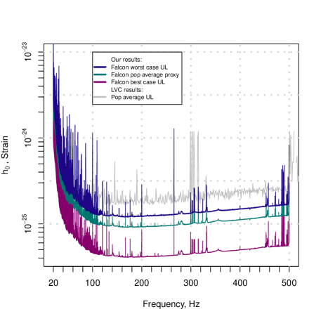
Figure 1: Gravitational wave intrinsic amplitude $h_{0}$ upper limits at 95% confidence as a function of signal frequency. The upper limits are a measure of the sensitivity of the search. We compare with the latest LIGO/Virgo all-sky results in this frequency range lvc_O2_allsky , which are a factor $\gtrsim$ 2 less constraining than ours, albeit able to detect sources with much larger distortions.

II The search and the parameter space

We use LIGO O2 open data losc ; o2_data ; o2_data2 . Our search looks for signals that are phase coherent over a certain time-span, called the coherence-length, and that evolve slowly over longer timescales. The search detects with highest efficiency IT2 signals. In O2_falcon2 we introduced the notion of the “IT2 model signal” for continuous gravitational wave signals because in the literature this signal model is used as a reference to measure search performance, and for upper limits. These are signals with constant amplitude and a frequency evolution that can be described by a Taylor expansion of order 2 around nominal frequency and frequency derivative values, see for example Section II of Jaranowski:1998qm . The “I” indicates the source being isolated and “T2” indicates an intrinsic frequency evolution given by a Taylor polynomial of degree 2.

Our target frequency range of 20-500 Hz is particularly difficult to analyze because of a multitude of detector artifacts, including combs below 100 Hz. Furthermore, for the same physical distortion of the neutron star, the putative signals are weaker at these frequencies, compared to higher frequencies.

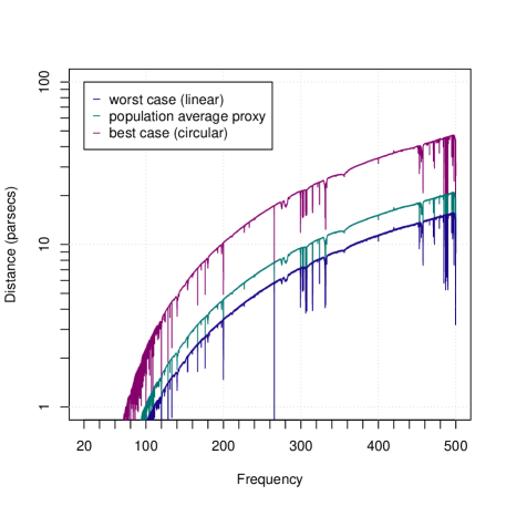
Figure 2: Reach of the search for stars with ellipticity of $10^{-8}$. The search is also sensitive to sources with ellipticities of $10^{-7}$ with a distance from Earth that is 10 times higher. The X axis is the gravitational wave frequency, which is twice the pulsar rotation frequency for emission due to an equatorial ellipticity. R-modes and other emission mechanisms give rise to emission at different frequencies. The top curve (purple) shows the reach for a population of circularly polarized sources; The middle curve (cyan) holds for a population of sources with random orientations; The bottom curve (blue) holds for linearly polarized sources.

In order to overcome this, we increase the sensitivity of the Falcon pipeline by using long coherence lengths at all stages of the search, as shown in Table 1. Regions of parameter space associated with high SNR results are searched again with progressively longer coherence length.

With these choices we would be able to see sources with ellipticity of $10^{-8}$ up to 44 pc away (Figure 2). The frequency derivative search range ($\pm 3\times 10^{-13}$ Hz/s) has been chosen to accommodate sources with ellipticities of $10^{-7}$. These sources could be seen up to a distance of $440$ pc.

Stage	Coherence length (days)	Minimum SNR
1	$2$	$6$
2	$3$	$9$
3	$4$	$11$
4	$6$	$12$
5	$9$	$16$
6	$16$	$16$
7	$16$	$16$

Table 1: Parameters for each stage of the search. Stage 7 refines outlier parameters by using denser sampling of parameter space, and then subjects them to an additional consistency check by comparing outlier parameters from analyses of individual interferometer data.

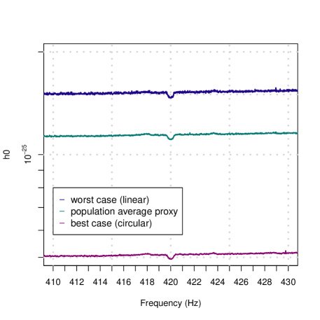
Figure 3: One of anomalies in our upper limits due to errors in public data. At these high frequencies the shot noise is dominant. A 60 Hz power line harmonic can add to it, but a dip below the shot noise is completely unphysical. We suspect that the origin of this type of feature is the cleaning procedure applied to the publicly released data. We would very much like the opportunity to understand and fully characterize this effect, as we explain in the text.

III Anomalies in O2 data

The O2 LIGO data have been cleaned. The procedure removes a number of instrumental artifacts by regressing against instrumental channels. The original implementation O2_cleaning was fairly conservative and was designed for searches of transient signals.

The procedure was then applied more aggressively using a significantly higher number of instrumental channels. In this type of procedure overfitting is a danger. One of the signs of overfitting is the appearance of artificially low values in the cleaned data. We see examples of this in lvc_O2_allsky in the upper limit and in the power spectral density plots. The presence of these unphysical data points is known o2_linespecs . We find such systematic anomalies also in the upper limits from this search, Figure 3. An argument that the low data values at certain frequencies are unphysical can also be made based on general grounds: at high frequencies the main contribution to the noise floor is shot noise, and regressing against auxiliary channels recording measurements from, say, magnetometers and microphones, cannot reduce the noise below this level.

Our pipeline establishes strict upper limits, within the stated calibration uncertainty Cahillane:2017vkb . If “overcleaning” happens, it will also affect a signal in the data, and compromise our upper limit results, unless the calibration uncertainty is correspondingly increased. Actually, all upper-limit methods need to know what any systematic from the cleaning procedure is, over the searched frequency range.

A systematic underestimation of the noise level is also problematic when considering the search algorithms. Gravitational wave searches usually combine separate measurements with weights that down-weigh noisier periods. Data with artificially low noise skew the weights and give more importance to unphysical data. The effect shown in Figure 3 is small and, if that is all that happens, we could simply excise affected bands.

In general we are concerned that whatever is causing the low-noise anomalies, has not been fully characterized and understood and hence could be affecting the data in subtle ways, without leaving such a visible signature, but still impacting the search results. If the auxiliary channels used to produce the cleaned data were publicly available, we would try and characterize features and magnitude of this effect and fold it in our strict upper limit values. In the absence of this, we present our upper limits taking the data at face value, but with the caveats explained in this Section.

IV Results

SNR	$f$	$\dot{f}$	$\textrm{RA}_{\textrm{J}2000}$	$\textrm{DEC}_{\textrm{J}2000}$	Comment
	Hz	pHz/s	degrees	degrees
$7417.8$	$265.57535$	$-1.0$	$71.591$	$-56.223$	Injection ip0
$6383.7$	$31.42473$	$-0.5$	$285.078$	$-58.269$	Injection ip11
$3712.5$	$52.80832$	$-0.2$	$302.538$	$-83.843$	Injection ip5
$1895.0$	$26.33722$	$-0.9$	$234.716$	$41.244$	Injection ip10
$1497.4$	$108.85716$	$0.0$	$178.369$	$-33.439$	Injection ip3
$27.1$	$83.43998$	$0.3$	$233.838$	$-41.127$
$27.0$	$59.99418$	$0.6$	$211.421$	$-21.567$	60 Hz line
$25.2$	$60.02252$	$-0.2$	$25.723$	$37.383$	60 Hz line
$25.1$	$80.40734$	$-0.9$	$225.641$	$77.846$	Line in H1
$21.9$	$465.58924$	$0.6$	$87.318$	$50.980$
$21.9$	$197.87552$	$-0.8$	$276.984$	$-62.431$
$21.6$	$400.01133$	$0.0$	$66.157$	$89.153$	Coincident lines
$21.6$	$31.84219$	$0.6$	$272.835$	$67.366$
$21.5$	$449.50129$	$0.7$	$308.074$	$-32.371$
$21.3$	$55.60198$	$0.7$	$218.116$	$-68.806$
$21.2$	$160.49660$	$0.5$	$90.941$	$32.384$	Line in L1
$21.0$	$140.26640$	$0.7$	$179.620$	$-19.718$	Line in H1
$21.0$	$357.19349$	$-0.6$	$202.263$	$-27.984$
$21.0$	$153.87728$	$-0.2$	$29.374$	$-53.913$	Line in H1
$21.0$	$440.03835$	$0.5$	$301.795$	$23.622$
$20.8$	$31.70025$	$-1.1$	$101.926$	$-66.112$	Line in H1
$20.8$	$260.10055$	$-0.5$	$85.537$	$17.565$
$20.7$	$180.10461$	$-0.8$	$122.697$	$-77.297$	60 Hz harmonic
$20.6$	$307.28973$	$1.1$	$330.582$	$28.601$	Near L1 line
$20.6$	$441.11365$	$-0.1$	$343.747$	$-58.935$
$20.6$	$442.38421$	$-0.0$	$20.788$	$-50.078$
$20.5$	$312.31246$	$0.6$	$284.115$	$-42.329$
$20.5$	$427.73851$	$0.8$	$259.995$	$-44.007$
$20.5$	$456.66685$	$0.8$	$161.618$	$67.993$	Broad line in H1
$20.4$	$457.11691$	$-0.0$	$147.143$	$44.056$	Broad line in H1
$20.4$	$245.06138$	$1.0$	$49.632$	$12.941$
$20.3$	$66.89584$	$0.8$	$177.962$	$-21.334$
$20.2$	$448.02463$	$0.8$	$263.539$	$46.220$
$20.2$	$153.97881$	$-0.5$	$131.683$	$-58.036$	Line in H1
$20.2$	$459.31715$	$0.0$	$341.763$	$20.999$
$20.2$	$192.60299$	$-0.6$	$340.182$	$50.884$
$20.1$	$394.38609$	$-0.1$	$257.670$	$-82.979$
$20.1$	$478.98702$	$0.3$	$151.593$	$-67.970$	Line in L1
$20.1$	$317.99684$	$-1.0$	$26.269$	$-22.945$
$20.0$	$436.12088$	$-1.3$	$342.703$	$-40.723$

Table 2: High SNR outliers produced by the detection pipeline. We list outliers with SNR above 20, and exclude those near ecliptic poles and associated with stationary lines. Only the highest-SNR outlier is shown for each 0.1 Hz frequency region. Outliers marked “ipX” are due to simulated signals “hardware-injected” during the science run for validation purposes. Their parameters are listed in Table 3. Outliers marked with “line” have strong narrowband disturbances near the outlier frequency. Signal frequencies refer to GPS epoch $1176425033$. Full list of outliers down to SNR$>16$ is available in data .

Label	Frequency	Spindown	$\textrm{RA}_{\textrm{J}2000}$	$\textrm{DEC}_{\textrm{J}2000}$
	Hz	pHz/s	degrees	degrees
ip0	$265.575343$	$-4.15$	$71.55193$	$-56.21749$
ip3	$108.857159$	$-1.46\times 10^{-5}$	$178.37257$	$-33.4366$
ip5	$52.808324$	$-4.03\times 10^{-6}$	$302.62664$	$-83.83914$
ip6	$145.860492$	$-6730$	$358.75095$	$-65.42262$
ip8	$190.634274$	$-8650$	$351.38958$	$-33.41852$
ip10	$26.338016$	$-85$	$221.55565$	$42.87730$
ip11	$31.424735$	$-0.507$	$285.09733$	$-58.27209$
ip12	$38.764787$	$-6250$	$331.85267$	$-16.97288$

Table 3: Parameters of the hardware-injected simulated continuous wave signals during the O2 data run (GPS epoch $1176425033$).

Based on the search results, we constrain the intrinsic strength $h_{0}$ of signals at the detectors. The $h_{0}$ upper limits also hold if a signal is present at a detectable level. In fact, in the band hosting loud outliers, for example due to the hardware injections, the upper limit values are higher than elsewhere.

In order to present the results in a concise way, each upper limit holds for signals with frequency from a certain frequency band, the whole sky and with spin-down values within the search range. This is completely standard practice in presenting continuous wave search results EHO2 ; lvc_O2_allsky ; O2_falcon2 . Details on the specific procedure that we use – the universal statistics algorithm – may be found in universal_statistics ; here we recap the main features.

The universal statistics algorithm establishes robust upper limits on the power of a single putative signal given a set of independent power measurements. The sets of power measurements are computed after filtering the data for each combination of frequency evolution parameters, sky position and polarization. Each measurement is then associated with 95% confidence level upper limit on signal amplitude. Because this procedure does not require injections it is computationally efficient to iterate over the entire parameter space. However, the volume of data produced is very large and the upper limits are aggregated by taking the maximum over marginalized parameters. A correction is applied to account for mismatch due to parameter space sampling. The upper limits are verified with Monte-Carlo injections.

The upper limit procedure is performed in narrow bands assuming that the input data have been perfectly calibrated. In reality, the calibration of the input data can be wrong in amplitude and phase Cahillane:2017vkb , but this varies slowly over frequency and can be assumed constant in each upper-limit band. The amplitude uncertainty simply translates in an uncertainty in the upper limit of the same magnitude, while the phase uncertainty is negligible.

Because we take the least favourable sky position and polarisation, the upper limit is the “worst-case” upper limit, and generally a signal will not need to be that loud to match our observation. The worst-case upper limits are in this sense conservative, but it is precisely because of this that they are strict upper limits, that hold true for any signal parameter combination. We also quote a “best-case” upper limit that corresponds to a population of circularly polarized signals, but still from the least favourable sky position.

It is common in the literature EHO2 ; lvc_O2_allsky to compute instead population-average upper limits, which do not hold at the given confidence for the least favourable signal parameter combinations. In order to ease comparison of our results with other methods, we compute a population-average proxy using a weighted sum of polarization-specific upper limits. We found that signals injected at the population average proxy level have between 90-95% chance of being recovered depending on the contamination of the underlying data by detector artifacts.

The gravitational wave amplitude upper limits from this search are shown in Figure 1 and are available in machine readable format at data .

Our upper limits can be translated into limits on gravitational waves from boson condensates around black holes boson1 ; boson2 , which are expected to emit monochromatic continuous wave signals discovering_axions with very small frequency drift. We leave it to the interested reader to constrain from our upper limits physical quantities of interest, based on the specific model they wish to consider (for example, an ensemble signal of Zhu:2020tht ).

The search also identifies small areas of parameter space containing waveforms that are unusually consistent with the data. These are the outliers of the search. The outliers are often caused by signals of terrestrial origin due to technical or environmental noise sources; the weaker ones may also be fluctuations. A key result of our search is a number of interesting outliers (Table IV), many of which are located in bands with clean frequency spectrum. Table IV only lists outliers with SNR above 20 and excludes outliers near ecliptic pole most likely associated with instrumental lines, in particular the outliers from the 0.5 Hz frequency comb. The full list of outliers down to SNR 16 is available in data .

Monte Carlo simulations show that we detect IT2 signals within $8\times 10^{-6}$ Hz of the signal frequency $f$, within $10^{-12}$ Hz/s of its frequency derivative, and within $0.12\textrm{\,Hz}/f$ radians from its sky location, the last calculated after projection on the ecliptic plane (“ecliptic distance”). For non-IT2 signals, or signals with frequency derivative outside search range, the tolerances should be widened. In particular, there is a degeneracy between sky location and frequency derivative, so a mismatch in the latter results in outlier offset from its true position on the sky.

Because the coherence length of our followup stage has been extended to 16 days, we have much tighter tolerance for the signals that pass our pipeline compared with previous searches. While we see 5 simulated signals clearly (ip0, ip3, ip5, ip10 and ip11, Table 3), the injections ip6 and ip12 do not produce any outliers as their frequency derivative smaller than $-5\times 10^{-9}$ Hz/s is well beyond our target parameter space. ip8 is loud enough to induce weak outliers with SNR below 20 even though its spindown is also outside of our target parameter space. The ip8 outliers are included in the supplemental materials file.

V Conclusions

We have performed the most sensitive search for continuous gravitational waves in the frequency band of 20-500 Hz. Just as in our previous papers O2_falcon ; O2_falcon2 , we have a number of interesting outliers. Our constraints are tighter than before, the signal-to-noise ratio is higher. Are they due to some sort of noise? Or are we seeing astrophysical sources? The latter is unlikely if we assume a classic IT2 source with ellipticity of $10^{-8}$ - we simply do not expect that many sources within 44 pc. Even widening the reach to 440 pc by including ellipticities of $10^{-7}$, it would be surprising that this many outliers are of astrophysical origin.

In order to make solid prediction on the number of detectable sources, one would need to have a mechanism that guarantees equatorial ellipticity in some minimal number of neutron stars rotating between a few tens and a few hundreds of Hz. We are not aware of any papers that provide such lower bounds, though there are efforts to characterise source populations under various assumptions population1 ; population2 . On the other hand, based on the null results of many different continuous wave searches, including all-sky surveys, directed searches and targeted searches - the latter probing significantly lower gravitational wave amplitude values than an all-sky search - a reasonable aspiration for results from an all-sky search is to find one signal.

We look forward to more data for further analysis.

- (1)
- (2) P. Jaranowski, A. Krolak and B. F. Schutz, “Data analysis of gravitational - wave signals from spinning neutron stars. 1. The Signal and its detection,” Phys. Rev. D 58 (1998), 063001
- (3) V. Dergachev, M. A. Papa, “Results from the first all-sky search for continuous gravitational waves from small-ellipticity sources”, Phys. Rev. Lett. 125, no.17, 171101 (2020)
- (4) V. Dergachev, M. A. Papa, “Results from high-frequency all-sky search for continuous gravitational waves from small-ellipticity sources”, Phys. Rev. D 103, 063019 (2021)
- (5) F. Gittins, N. Andersson and D. I. Jones, “Modelling neutron star mountains,” [arXiv:2009.12794 [astro-ph.HE]].
- (6) G. Woan, M. D. Pitkin, B. Haskell, D. I. Jones, and P. D. Lasky, Evidence for a Minimum Ellipticity in Millisecond Pulsars, ApJL 863 L40 (2018)
- (7) Detectability of continuous gravitational waves from isolated neutron stars in the Milky Way: the population synthesis approach, Marek Cieślar, Tomasz Bulik, Małgorzata Curyło, Magdalena Sieniawska, Neha Singh, Michał Bejger, arXiv:2102.08854
- (8) Modeling the Galactic Neutron Star Population for Use in Continuous Gravitational Wave Searches Brendan T. Reed, Alex Deibel, C. J. Horowitz, arXiv:2104.00771
- (9) Karl Wette, Liam Dunn, Patrick Clearwater, Andrew Melatos, Deep exploration for continuous gravitational waves at 171–172 Hz in LIGO second observing run data, arXiv:2103.12976
- (10) B. P. Abbott et al. (LIGO Scientific Collaboration and Virgo Collaboration), All-sky search for continuous gravitational waves from isolated neutron stars using Advanced LIGO O2 data, Phys. Rev. D 100 024004 (2019).
- (11) B. Steltner, M. A. Papa, H. B. Eggenstein, B. Allen, V. Dergachev, R. Prix, B. Machenschalk, S. Walsh, S. J. Zhu and S. Kwang, “Einstein@Home All-sky Search for Continuous Gravitational Waves in LIGO O2 Public Data,” Astrophys. J. 909, no.1, 79 (2021) doi:10.3847/1538-4357/abc7c9
- (12) V. Dergachev and M. A. Papa, “Sensitivity improvements in the search for periodic gravitational waves using O1 LIGO data,” Phys. Rev. Lett. 123, no.10, 101101 (2019) doi:10.1103/PhysRevLett.123.101101 [arXiv:1902.05530 [gr-qc]].
- (13) V. Dergachev, On blind searches for noise dominated signals: a loosely coherent approach, Class. Quantum Grav. 27, 205017 (2010).
- (14) V. Dergachev, Loosely coherent searches for sets of well-modeled signals, Phys. Rev. D 85, 062003 (2012)
- (15) V. Dergachev, Loosely coherent searches for medium scale coherence lengths, arXiv:1807.02351
- (16) M. Vallisneri et al. The LIGO Open Science Center, proceedings of the 10th LISA Symposium, University of Florida, Gainesville, 2015 J. Phys.: Conf. Ser. 610 012021
- (17) LIGO Open Science Center, https://doi.org/10.7935/CA75-FM95, (2019)
- (18) O2 Instrumental Lines https://www.gw-openscience.org/o2speclines/
- (19) R. Abbott et al. (LIGO Scientific Collaboration and Virgo Collaboration), Open data from the first and second observing runs of Advanced LIGO and Advanced Virgo, SoftwareX 13 (2021) 100658.
- (20) J.C. Driggers et al. (LIGO Scientific Collaboration Instrument Science Authors), Improving astrophysical parameter estimation via offline noise substraction for Advanced LIGO, Phys. Rev. D 99, 042001 (2019).
- (21) C. Cahillane, J. Betzwieser, D.A. Brown, E. Goetz, E.D. Hall, K. Izumi, S. Kandhasamy, S. Karki, J.S. Kissel, G. Mendell, R.L. Savage, D. Tuyenbayev, A. Urban, A. Viets, M. Wade, and A.J. Weinstein, Calibration uncertainty for Advanced LIGO?s first and second observing runs, Phys. Rev. D 96, 102001 (2017)
- (22) V. Dergachev, A Novel Universal Statistic for Computing Upper Limits in Ill-behaved Background, Phys. Rev. D 87, 062001 (2013).
- (23) See EPAPS Document No. [number will be inserted by publisher] for numerical values of upper limits, outlier tables and hardware injection parameters. Also at https://www.aei.mpg.de/continuouswaves/O2Falcon20-500
- (24) M. Baryakhtar, R. Lasenby, M. Teo, Black Hole Superradiance Signatures of Ultralight Vectors, Phys. Rev. D 96, 035006s (2017)
- (25) A. Arvanitaki, M. Baryakhtar, R. Lasenby, S. Dimopoulos, S. Dubovsky, Black Hole Mergers and the QCD Axion at Advanced LIGO, Phys. Rev. D 95, 043001 (2017)
- (26) A. Arvanitaki, M. Baryakhtar, and X. Huang, Discovering the QCD axion with black holes and gravitational waves, Phys. Rev. D 91, 084011 (2015)
- (27) S. J. Zhu, M. Baryakhtar, M. A. Papa, D. Tsuna, N. Kawanaka and H. Eggenstein, Characterizing the continuous gravitational-wave signal from boson clouds around Galactic isolated black holes, Phys. Rev. D 102, 063020 (2020)