A New Fast Monte Carlo Code for Solving Radiative Transfer Equations based on Neumann Solution

Abstract

In this paper, we proposed a new Monte Carlo radiative transport (MCRT) scheme, which is based completely on the Neumann series solution of Fredholm integral equation. This scheme indicates that the essence of MCRT is the calculation of infinite terms of multiple integrals in Neumann solution simultaneously. Under this perspective we redescribed MCRT procedure systematically, in which the main work amounts to choose an associated probability distribution function (PDF) for a set of random variables and the corresponding unbiased estimation functions. We can select a relatively optimal estimation procedure that has a lower variance from an infinite possible choices, such as the term by term estimation. In this scheme, MCRT can be regarded as a pure problem of integral evaluation, rather than as the tracing of random walking photons. Keeping this in mind, one can avert some subtle intuitive mistakes. In addition the $\delta$-functions in these integrals can be eliminated in advance by integrating them out directly. This fact together with the optimal chosen random variables can remarkably improve the Monte Carlo (MC) computational efficiency and accuracy, especially in systems with axial or spherical symmetry. An MCRT code, Lemon(Linear Integral Equations’ Monte Carlo Solver Based on the Neumann solution), has been developed completely based on this scheme. Finally, we intend to verify the validation of Lemon, a suite of test problems mainly restricted to flat spacetime have been reproduced and the corresponding results are illustrated in detail.

1. Introduction

Radiative transfer (RT) constantly plays an important role in astrophysical researches. It can not only give us the emergent spectra and light curves of various astrophysical systems directly but also participate the co-evolution of these systems indispensably. Naturally, RT process is completely dictated and described by the radiative transfer equation (RTE), which is an integro-differential equation when the scattering contributions are taken into account (Chandrasekhar, 1960; Pomraning, 1973). To solve RTE, various methods have been proposed over the last decades (Lindquist, 1966; Connors et al., 1980; Gorecki & Wilczewski, 1984; Hauschildt & Wehrse, 1991; Haardt, 1993; Poutanen & Svensson, 1996a; Zane et al., 1996; Böttcher & Liang, 2001; Dolence et al., 2009; Yuan et al., 2009; Gammie & Leung, 2012; Dexter et al., 2010; Schnittman & Krolik, 2010; Younsi et al., 2012; Schnittman & Krolik, 2013; Dexter, 2016; Takahashi & Umemura, 2017; Ryan & Dolence, 2020). Roughly speaking, these methods can be classified as analytical (López Ariste & Semel, 1999; Semel & López Ariste, 1999) and numerical (Janett et al., 2017a, b; Janett, 2019) ones.

The most relevant and widely used numerical method is MC method due to its remarkable simplicity and powerful efficiency in dealing with high-dimensional integrations (Pozdnyakov et al., 1983; Whitney, 2011; Noebauer & Sim, 2019), which is crucial to solve RTE. Especially, the accuracy of the MC method is only dependant on the sample size: N, but it is irrelevant with the dimension of the system. The MC method can deal with complicated problems provided it can be converted into probability ones with given PDFs. Usually the sampling algorithms of MC method are very simple and can be easily implemented by a program language. Even though with these virtues, the results produced by the MC method have a famous $N^{-1/2}$ convergent rate, which is quite low and means that a relatively higher accuracy needs a sufficient large set of samples.

The MC method is introduced mainly to treat the RT problems with scattering processes incorporated, which are dictated by the differentia-integral equations. Up to now, a lot of works based upon the MC method dedicated to solve such equations (which are even though not provided explicitly in these works) have been done (Connors et al., 1980; Stern et al., 1995; Hua, 1997; Dolence et al., 2009; Schnittman & Krolik, 2013; Ryan et al., 2015; Zhang et al., 2019; Mościbrodzka, 2020). Very early, Connors et al. (1980) used the MC method to trace the polarized RT around a Kerr black hole and calculated the spectra emerging from a hot electron cloud and accretion disk. They adopted the Walker-Penrose (Walker & Penrose (1970)) complex constant to calculate the parallel transported polarization vector. This scheme was widely used in polarized RT later. Dolence et al. (2009) proposed a new scheme and developed a public available code: grmonty, aiming to calculate the unpolarized synchrotron spectra of hot plasmas with Compton scattering considered in full general relativity. In grmonty, the superphoton, also called as ”photon packets”, plays a key role. Later, the scheme of grmonty, especially the scenario of superphoton, was fully adopted by the codes: bhlight (Ryan et al., 2015) and Pandurata (Schnittman & Krolik, 2013). Pandurata is an MC code aiming for polarized radiation transport around Kerr black holes, including arbitrary emission and absorption effects, as well as electron scattering. In Pandurata the superphotons have broadband energies, while in grmonty they are monoenergetic (Schnittman & Krolik, 2013). In order to implement a more self-consistent calculations of Comptonised energy spectra for extended coronae in Kerr spacetime, an MC polarized RT code, monk, has been developed by Zhang et al. (2019).

The descriptions of these codes and many other analogous ones are in a very physical intuitive manner, i.e., emitting a superphoton, then randomly tracing it until either it escapes from the radiative region or is absorbed by the medium. Of course, during the propagation, the photon experienced Compton scattering and absorption in the media. In this physical intuitive description, the RTE seems unimportant and is rarely mentioned. But one will see later that this is not true and we believe that the importance of RTE has been underestimated in the former works in some sense.

In contrast, an RTE without scattering is a differential equation and can usually be solved based on the ray-tracing approach, rather than the MC method (Broderick & Blandford, 2003; Li et al., 2009; Huang & Shcherbakov, 2011; Chen et al., 2015; Dexter, 2016; Meliani et al., 2017; Pihajoki et al., 2017, 2018; Mościbrodzka & Gammie, 2018; Bronzwaer et al., 2018; Chan et al., 2019; Tsunetoe et al., 2020; Vincent et al., 2020). In curved spacetime, the geodesics along which the radiation propagates (also including the polarization vector if the radiation is polarized) should be solved simultaneously. Hence a fast and accuracy geodesic solver is crucial (Dexter & Agol, 2009; Dauser et al., 2010; Vincent et al., 2011; Yang & Wang, 2013). Unlike the scattering incorporated cases, the RTE plays a central role in these works and is given explicitly.

There are two different paradigms when tracing a radiation, i.e., emitter-to-observer (Cunningham, 1975; Rauch & Blandford, 1994; Broderick & Blandford, 2003; Dovčiak et al., 2004; Schnittman et al., 2006) and observer-to-emitter (Laor et al., 1990; Kojima, 1991; Dolence et al., 2009; Psaltis & Johannsen, 2012; Schnittman & Krolik, 2013). They are suitable for RT circumstances with and without scattering incorporated, respectively. In the emitter-to-observer framework, the transfer function is crucial and needs to be evaluated numerically and tabulated in advance to obtain the observational quantities at infinity (Cunningham, 1975; Laor et al., 1990).

When one deals with polarized radiation transport, polarization vector is a relevant concept (Chandrasekhar, 1960). In fact the Stokes parameters of $I,Q,U,V$ are determined up to a rotation in the plane perpendicular to the propagation direction of the radiation. If the reference frame in that plane is rotated anticlockwise by a angle $\phi$, the components $Q$ and $U$ will change as $Q^{\prime}=Q\cos 2\phi+U\sin 2\phi,U^{\prime}=-Q\sin 2\phi+U\cos 2\phi$. It means that we need a determined frame to fix the values of the Stokes parameters, which is equivalent to a single vector since the frame is in a plane. Hence we have to trace the polarization vector along the ray trajectory and the vector moves in a parallel transport manner. In flat spacetime, a parallel transported vector remains unchanged, thus the tracing is trivial. While in curved spacetime, the parallel transport of a vector $\mathbf{f}=f^{\mu}\partial_{\mu}$ is determined by the equation $Df^{\mu}/d\lambda=df^{\mu}/d\lambda+\Gamma^{\mu}_{\alpha\beta}f^{\alpha}k^{\beta}=0$, where $Df^{\mu}/d\lambda$ is the covariant derivative, $\lambda$ and $k^{\beta}$ are the affine parameter and tangent vector of the trajectory, respectively. Solving these equations numerically is time consuming (Chen et al., 2015). In Kerr spacetime, due to the existence of the complex-valued Wolker-Penrose constant $k_{\text{wp}}$ (Walker & Penrose, 1970) and the conditions of $\mathbf{f}\cdot\mathbf{f}=1$ and $\mathbf{f}\cdot\mathbf{k}=0$, the whole problem amounts to solve a set of linear algebraic equations (Connors & Stark, 1977; Connors et al., 1980).

In curved spacetime, the parallel transport of polarization vector can be incorporated into the polarized RTEs through several different but equivalent formalisms. For example, Shcherbakov & Huang (2011) developed a mechanism, in which a orthogonal tetrad was parallel transported along the ray from the observer to the black hole, and the coefficient matrix of absorption, Faraday rotation and conversion was modified by a rotation. Latter, Gammie & Leung (2012) proposed a more generic formalism and demonstrated the equivalence of approaches adopted by Broderick & Blandford (2003, 2004), Schnittman & Krolik (2010) and Shcherbakov & Huang (2011). These formalisms were recently employed by many authors (Dexter, 2016; Jiménez-Rosales & Dexter, 2018; Pihajoki et al., 2018; Mościbrodzka & Gammie, 2018; Tsunetoe et al., 2020; Dexter et al., 2020) to obtain more predictable features for polarized RT in complicated GRMHD simulations, which could potentially impose more precise constrains on the high quality observational data. One may notice that in all those works, the scattering process was not included. Thus for the RT without scattering, the RTE plays an essential role and is usually solved by a non-MC method. But for the RT with scattering, the MC method is employed and described in a quite physically intuitive manner, and the RTEs are mentioned rarely. Motivated by this unsymmetrical and unsatisfactory situation for the RTEs and MC method, we intend to develop an RT scheme which employs the MC method and RTEs equally and simultaneously, or a MCRT scheme based upon the RTEs. As we will see that the RT without scattering can also be solved by this new scheme appropriately, even though not so efficiently.

This motivation is also inspired by several other reasons. First, the MC method initially introduced in the RT aims to evaluate the infinite terms of multiple integrals in the Neumann solution of RTE (Davison, 1957). Regarding MC method from this mathematical perspective can remarkably improve the calculation efficiency and accuracy compared to the superphoton scheme. Second, since the whole work is integral evaluation, we are flexible to choose various PDFs for sampling and weight functions for unbiased estimations. These choices are equivalent but with different computational efficiency and variance. Therefore we can select a relatively optimal PDF to improve the accuracies of integral evaluation. Especially our scheme can avoid subtle mistakes that may be caused by physical intuitions. Third, the RTE and its Neumann solution are oriented in our scheme. They are also the starting point of the whole framework. If the RTE can be greatly simplified at the very beginning under a given condition, such as the axial symmetry of the system, the corresponding MC sampling procedure will be simplified as well. And the PDFs for scattering sampling could be totally nonphysical but mathematically correct.

This paper is organized as follows. In section 2, we give a detailed description of our scheme built upon the RTE and its Neumann solution, including the sampling procedures for position transport, scattering and observational quantity estimations. Next we extend this scheme to deal with polarized radiative transfer processes in Section 3. We verify our scheme through its applications in various radiative transfer problems in Section 4. Finally a brief discussion on our scheme and its limitations is presented in Section 5.

2. Methods

In this section we will illustrate the scheme through a simple example, which contains all relevant ingredients. We will demonstrate that the observational quantities can be expressed as an infinite series of multiple integrals via the Neumann solution and the MC method is introduced for evaluating these integrals.

2.1. Neumann Series Solution and Recording Function

The RT is essentially a particle transport process described exactly by the Boltzmann’s equation (BE). Therefore an RTE is actually identical with a BE. The difference is that the particles (here is photon) do not interact with each other except acting with the external medium. We also do not consider the inducing process causing the RTE to be non-linear (Pomraning, 1973). Taking the function $N(\nu,\mathbf{\Omega},\mathbf{r})$ to describe the photon number of unpolarized radiation distributed over position $\mathbf{r}$, frequency $\nu$ and direction $\mathbf{\Omega}$. Without lost of generality, we assume that the radiative field is time independent, the RTE simply reads (Pomraning, 1973)

$$\begin{split}&\mathbf{\Omega}\cdot\nabla N(\nu,\mathbf{\Omega},\mathbf{r})+\sigma(\nu,\mathbf{\Omega},\mathbf{r})N(\nu,\mathbf{\Omega},\mathbf{r})=S(\nu,\mathbf{\Omega},\mathbf{r})\displaystyle\\ &+\int_{0}^{\infty}\int_{4\pi}\sigma_{s}(\nu^{\prime}\rightarrow\nu,\mathbf{\Omega}^{\prime}\rightarrow\mathbf{\Omega},\mathbf{r})N(\nu^{\prime},\mathbf{\Omega}^{\prime},\mathbf{r})d\nu^{\prime}d\mathbf{\Omega}^{\prime},\end{split}$$ (1)

where $\sigma=\sigma_{a}+\sigma_{s}$, $\sigma_{a}$ and $\sigma_{s}$ are the absorption and scattering coefficients, respectively and

$$\begin{split}&\sigma_{s}(\nu^{\prime},\mathbf{\Omega}^{\prime})=\int\sigma_{s}(\nu^{\prime}\rightarrow\nu,\mathbf{\Omega}^{\prime}\rightarrow\mathbf{\Omega},\mathbf{r})d\nu d\mathbf{\Omega}.\end{split}$$ (2)

$S(\nu,\mathbf{\Omega},\mathbf{r})$ is the emissivity of the medium. Eq. (1) is an integro-differential equation. In order to solve it numerically by the MC method, we need to recast it into an integral equation. To accomplish this, we define the right hand side of Eq. (1) as an auxiliary quantity $\mathbf{\psi}$, i.e.,

$$\begin{split}&\displaystyle\mathbf{\psi}(\nu,\mathbf{\Omega},\mathbf{r})=S(\nu,\mathbf{\Omega},\mathbf{r})\displaystyle\\ &+\int_{0}^{\infty}\int_{4\pi}\sigma_{s}(\nu^{\prime}\rightarrow\nu,\mathbf{\Omega}^{\prime}\rightarrow\mathbf{\Omega},\mathbf{r})N(\nu^{\prime},\mathbf{\Omega}^{\prime},\mathbf{r})d\nu^{\prime}d\mathbf{\Omega}^{\prime}.\end{split}$$ (3)

Obviously $\mathbf{\psi}$ represents the total photon number flux of the radiation field at a given point, direction and frequency. Taking $\mathbf{\psi}$ as a quantity already known and solving Eq. (1) formally, we have (Pomraning, 1973)

$$\begin{split}&\displaystyle N(\nu,\mathbf{\Omega},\mathbf{r})=\int_{0}^{|\mathbf{r}-\mathbf{r}_{0}|}\psi\left(\nu,\mathbf{\Omega},\mathbf{r}-s\mathbf{\Omega}\right)\\ &\times\exp\left(-\int^{s}_{0}\sigma\left(\nu,\mathbf{\Omega},\mathbf{r}-s^{\prime}\mathbf{\Omega}\right)ds^{\prime}\right)ds.\end{split}$$ (4)

This expression is very useful and its physical implication is explicit, i.e., the photon number density at a given place and direction equals the contributions of $\psi$ integrated along the ray backward with a exponential attenuation factor multiplied at each point, in which the factor accounts for the absorption and scattering effects. Substituting Eq. (4) into Eq. (3) to eliminate $N(\nu,\mathbf{\Omega},\mathbf{r})$, we obtain an integral equation for $\psi$

$$\begin{split}\mathbf{\psi}&\displaystyle(\nu,\mathbf{\Omega},\mathbf{r})=S(\nu,\mathbf{\Omega},\mathbf{r})\displaystyle+\int_{0}^{\infty}d\nu^{\prime}\int_{4\pi}d\mathbf{\Omega}^{\prime}\int_{0}^{\infty}ds\\ &\times\psi\left(\nu^{\prime},\mathbf{\Omega}^{\prime},\mathbf{r}-s\mathbf{\Omega}^{\prime}\right)\sigma_{s}(\nu^{\prime}\rightarrow\nu,\mathbf{\Omega}^{\prime}\rightarrow\mathbf{\Omega},\mathbf{r})\\ &\times\exp\left(-\int^{s}_{0}\sigma\left(\nu^{\prime},\mathbf{\Omega}^{\prime},\mathbf{r}-s^{\prime}\mathbf{\Omega}^{\prime}\right)ds^{\prime}\right).\end{split}$$ (5)

To simplify the above equation, we introduce the normalized scattering and transport kernels denoted by $C$ and $T_{s}$, and

$$\begin{split}&\displaystyle C(\nu^{\prime}\rightarrow\nu,\mathbf{\Omega}^{\prime}\rightarrow\mathbf{\Omega}|\mathbf{r})=\frac{\sigma_{s}(\nu^{\prime}\rightarrow\nu,\mathbf{\Omega}^{\prime}\rightarrow\mathbf{\Omega},\mathbf{r})}{\sigma_{s}(\nu^{\prime},\mathbf{\Omega}^{\prime},\mathbf{r})},\end{split}$$ (6)

$$\begin{split}T_{s}(\mathbf{r}_{s}\rightarrow\mathbf{r}&|\nu^{\prime},\mathbf{\Omega}^{\prime})=\displaystyle\frac{1}{A}\sigma_{s}(\nu^{\prime},\mathbf{\Omega}^{\prime},\mathbf{r})\\ &\times\exp\left(-\int^{s}_{0}\sigma_{s}\left(\nu^{\prime},\mathbf{\Omega}^{\prime},\mathbf{r}_{s^{\prime}}\right)ds^{\prime}\right),\end{split}$$ (7)

where $\mathbf{r}_{s}=\mathbf{r}-s\mathbf{\Omega}^{\prime}$ and $A$ is the normalization factor for $T_{s}$. Since both $C$ and $T_{s}$ are normalized, they will be taken as PDFs for photon transport in momentum and position spaces respectively. For simplicity, we define the total transport kernel $K=T_{s}\cdot C\cdot w_{s}$, where $\displaystyle w_{s}=A\cdot\exp\left(-\int^{s}_{0}\sigma_{a}\left(\nu^{\prime},\mathbf{\Omega}^{\prime},\mathbf{r}_{s^{\prime}}\right)ds^{\prime}\right)$ is weight which will be used as estimation for observational quantity. Using the total absorption coefficient $\sigma$, we can choose another position transport function $T$ given by

$$\begin{split}&\displaystyle T(\mathbf{r}_{s}\rightarrow\mathbf{r}|\nu^{\prime},\mathbf{\Omega}^{\prime})=\\ &\frac{1}{A}\sigma(\nu^{\prime},\mathbf{\Omega}^{\prime},\mathbf{r})\exp\left(-\int^{s}_{0}\sigma\left(\nu^{\prime},\mathbf{\Omega}^{\prime},\mathbf{r}_{s^{\prime}}\right)ds^{\prime}\right),\end{split}$$ (8)

and the corresponding weight function $w=A\sigma_{s}/\sigma$. Also we have $K=T\cdot C\cdot w$. The two choices of $T$ correspond two different sampling algorithms for position transport. We prefer to choose $T_{s}$ and $w_{s}$ because they are more convenient for sampling. Meanwhile the effect of absorption is considered in the factor $w_{s}$. If we choose $T$ as the transport sampling PDF, the weight becomes $A\sigma_{s}/\sigma$ and $\sigma_{s}/\sigma$ is the probability that scattering happens.

If we denote $P=(\nu,\mathbf{\Omega},\mathbf{r})$, then Eq. (5) can be written as

$$\begin{split}&\displaystyle\psi(P)=S(P)+\int\psi\left(P^{\prime}\right)K(P^{\prime}\rightarrow P)dP^{\prime},\end{split}$$ (9)

which is mathematically called as the Fredholm integral equation of second kind. It is well known that Eq. (9) has the Neumann series solution, which can be given directly by (Davison, 1957)

$$\begin{split}&\displaystyle\psi(P)=\sum_{m=0}^{\infty}\psi_{m}(P),\end{split}$$ (10)

where

$$\begin{split}&\displaystyle\psi_{0}(P)=S(P),\\ &\displaystyle\psi_{1}(P)=\int_{P_{1}}\psi_{0}(P_{1})K(P_{1}\rightarrow P)dP_{1}\\ &=\int_{P_{1}}S(P_{1})K(P_{1}\rightarrow P)dP_{1},\\ &\displaystyle\psi_{2}(P)=\int_{P_{2}}\psi_{1}(P_{2})K(P_{2}\rightarrow P)dP_{2}\\ &=\int_{P_{1}}\int_{P_{1}}S(P_{1})K(P_{1}\rightarrow P_{2})K(P_{2}\rightarrow P)dP_{1}dP_{2},\\ &\cdots\\ &\displaystyle\psi_{m}(P)=\int_{P_{m}}\psi_{m-1}(P_{m})K(P_{m}\rightarrow P)dP_{m}\\ \end{split}$$ (11)

$$\begin{split}&=\int_{P_{1}}\cdots\int_{P_{m}}S(P_{1})K(P_{1}\rightarrow P_{2})K(P_{2}\rightarrow P_{3})\cdots\\ &K(P_{m}\rightarrow P)dP_{1}dP_{2}\cdots dP_{m}.\\ \end{split}$$

The Neumann solution has a very simple physical interpretation that the photon number flux of the radiation field at $P$ is the sum of all photons travel to there after zero, one, two and many times transportations.

To obtain the observed quantities at infinity in a special direction $\mathbf{\Omega}_{\text{obs}}$, such as the total photon number flux $F_{\text{obs}}$, we introduce the recording function $f(P)$ defined as

$$\begin{split}\displaystyle f(\nu,\mathbf{\Omega},\mathbf{r})=&\exp\left(-\int^{s}_{0}\sigma\left(\nu,\mathbf{\Omega},\mathbf{r}-s^{\prime}\mathbf{\Omega}\right)ds^{\prime}\right)\\ &\times\delta(\mathbf{\Omega}-\mathbf{\Omega}_{\text{obs}}).\end{split}$$ (12)

Noting Eq. (4), we have

$$\begin{split}I=\int_{P}\psi(P)f(P)dP.\end{split}$$ (13)

Substituting the Neumann solution into above equation, we obtain

$$\begin{split}\displaystyle I=\sum_{m=0}^{\infty}I_{m},\end{split}$$ (14)

where

$$\begin{split}&\displaystyle I_{m}=\int_{P_{1}}\cdots\int_{P_{m}}S(P_{1})K(P_{1}\rightarrow P_{2})K(P_{2}\rightarrow P_{3})\\ &\cdots\times K(P_{m}\rightarrow P)f(P)dP_{1}dP_{2}\cdots dP_{m}dP.\\ \end{split}$$ (15)

There are infinite number of multiple integrals needed to be evaluated simultaneously, this work can be done by MC method in an efficient way. In the next subsections, we will discuss the MC method and the procedure to evaluate those integrals in detail.

2.2. The Monte Carlo Method

The strategy of the MC to calculate an integral $I=\int_{a}^{b}f(x)dx$ is very simple, i.e., the integral $I$ is regarded as the expectation value of a random variable $y$ with a PDF: $p(y)$. On the other hand, the expectation value can be approximated by the algebraic average of a set of samples of $y$. Suppose that $y$ is a function of another random varible $x$, i.e., $y=g(x)$, then the PDF of $x$, $p(x)$ satisfies $p(y)dy=p(x)dx$. The expectation value of $y$ is given approximately by

$$\begin{split}&\displaystyle\int yp(y)dy=\int g(x)p(x)dx\approx\frac{1}{N}\sum_{i=1}^{N}g(x_{i}),\end{split}$$ (16)

where $x_{i}$ is a set of samples of $x$ obtained by sampling $p(x)$. Since $p(y)dy=p(x)dx$, $y_{i}=g(x_{i})$ are samples of $y$. Then one can split $f(x)$ as the product of two functions: $f(x)=g(x)p(x)$, where $p(x)$ is normalized and will be used as a PDF to generate a set of samples of $x$, we have

$$\begin{split}\displaystyle I=\int_{a}^{b}f(x)dx=\int_{a}^{b}g(x)p(x)dx\approx\frac{1}{n}\sum_{i=1}^{n}g(x_{i}).\end{split}$$ (17)

Notice that only $g(x)$ appears in the final expression, which is usually called as the weight or the unbiased estimation of $I$. The number of ways to split $f(x)$ is infinite. The various splitting has different computational efficiency and variance. But there exists an optimal choice for $f(x)\geq 0$, where $p(x)=f(x)/A$ and $A=\int f(x)dx$ is the normalization factor (if $f(x)$ can take negative values, the optimal choice is different), for this choice the variance is exactly vanished. But the problem is that we do not know $A$ in advance and its value is exactly what we want to calculate. It means that the optimal choice is impossible for practical implementation. However this result tells us that we should choose a $p(x)$ as similar with $f(x)$ as possible, the error will also be relatively smaller. This is the essence of the so-called important sampling.

2.3. Transport Game: an Example of Illustration

In the above section, we discuss how to calculate a single integral by the MC method. But the quantity we want to evaluate given in Eq. (14) is an infinite series of multiple integrals. To calculate these integrals simultaneously by the MC method, we need a similar but extended scheme. Such scheme has been extensively studied in nuclear physics sector, where neutron transport is heavily concerned (Davison, 1957). Goertzel (1958) proposed a novel and systematic strategy, called as transport game, to evaluate such a quantity. Spanier (1959) put this scheme on a stringent mathematical foundation and its validation can be proved by probability and measure theories.

① generate $P_{1}$ by sampling $S(P_{1})$,

② For any $l\geq 2$, compute $\tilde{p}(P_{l-1})=\displaystyle\int K(P_{l-1}\rightarrow P_{l})dP_{l}$ for a given $P_{l-1}$ and take $\tilde{p}(P_{l-1})$ as a survival probability,

③ If $\xi\leq\tilde{p}(P_{l-1})$ generate $P_{l}$ by sampling $\displaystyle\tilde{K}(P_{l}|P_{l-1})=\frac{K(P_{l-1}\rightarrow P_{l})}{\displaystyle\int K(P_{l-1}\rightarrow P_{l})dP_{l}}$,

Repeat steps ② and ③

④ If $\xi>\tilde{p}(P_{M})$, then terminate the game.

Algorithm 1 Steps of transport game

To illustrate how does the transport game work, we shall first demonstrate a toy model containing the key ingredients. The steps of the algorithm for the toy model are presented in Algorithm. 1. After implementing these steps, one can obtain a state sequence: $P_{1},P_{2},\cdots,P_{M}$. One of the weights associated with this algorithm is given by

$$\begin{split}&\displaystyle F_{1}=\frac{f(P_{M})}{1-\tilde{p}(P_{M})}.\end{split}$$ (18)

Now we will show that $F_{1}$ is an unbiased estimation of the photon number $I$. First, the probability corresponding to such a state sequence is obviously given by

$$\begin{array}[]{lll}&H(P_{1},P_{2},\cdots,P_{M})dV&\\ =&\displaystyle S(P_{1})\left(\prod_{l=2}^{M}\tilde{p}(P_{l-1})\tilde{K}(P_{l-1}\rightarrow P_{l})\right)\times(1-\tilde{p}(P_{M}))dV&\\ =&\displaystyle S(P_{1})\left(\prod_{l=2}^{M}K(P_{l-1}\rightarrow P_{l})\right)\times(1-\tilde{p}(P_{M}))dV,&\end{array}$$ (19)

where $dV=dP_{1}dP_{2}\cdots dP_{M}$. Thus the expectation value of $F_{1}$ for an explicit $M$ is given by

$$\begin{array}[]{lll}&\langle F_{1}\rangle_{M}=\displaystyle\int\cdots\int H(P_{1},P_{2},\cdots,P_{M})F_{1}(P_{M})dV&\\ =&\displaystyle\int\cdots\int S(P_{1})\displaystyle\left(\prod_{l=2}^{M}K(P_{l-1}\rightarrow P_{l})\right)f(P_{M})dV=I_{M}.&\end{array}$$ (20)

Then the average of $I$ is given by the sum of $\langle F_{1}\rangle_{M}$ for all $M$, i.e., $\displaystyle E[F_{1}]=\sum_{M=0}^{\infty}\langle F_{1}\rangle_{M}=\sum_{M=0}^{\infty}I_{M}=I$.

Similarly one can show that

$$\begin{split}&\displaystyle F_{2}=\displaystyle\sum_{m=1}^{M}f(p_{m}),\end{split}$$ (21)

is another unbiased estimation of $I$, i.e., $\displaystyle E[F_{2}]=\sum_{M=0}^{\infty}\langle F_{2}\rangle_{M}=\sum_{M=0}^{\infty}I_{M}=I$. $F_{1}$ and $F_{2}$ are called as the final event and item by item estimations of $I$, respectively. In addition, there are many other unbiased estimations of $I$. For example, we can modify Algorithm. 1 by introducing a weight factor $w$ and obtain Algorithm. 2,

① generate $P_{1}$ by sampling $S(P_{1})$ and set $w=1$;

② For any $l\geq 2$, compute $C(P_{l-1})=\displaystyle\int K(P_{l-1}\rightarrow P_{l})dP_{l}$ for a given $P_{l-1}$, and take $C(P_{l-1})$ as the normalization factor;

③ generate $P_{l}$ by sampling $\displaystyle\tilde{K}(P_{l}|P_{l-1})=\frac{1}{C(P_{l-1})}K(P_{l-1}\rightarrow P_{l}$);

④ Update $w$ as $w=w\cdot C(P_{l-1})$;

Repeat steps ②,  ③ and ④.

Algorithm 2 Steps of transport game

where, the unbiased estimations for $I$ is $F_{3}^{m}=w\cdot f(P_{m})$. In Algorithm. 2, the state sequence will not be truncated but with a decreased weight $w$.

We can also understand the transport game from the MC splitting scheme directly. Notice that the transport kernel is $K=T_{s}\cdot C\cdot w_{s}$, for the $m$-th term $I_{m}$ given by Eq. (15), we can separate a associated PDF for all random variables: $P_{1},\cdots,P_{m},P$ from the integrand as

$$\begin{split}&\displaystyle\widetilde{f}(P1,\cdots,P_{m},P)=S(P_{1})\cdot T_{s}(\mathbf{r}_{1}\rightarrow\mathbf{r}_{2})\cdot C(\nu_{1},\mathbf{\Omega}_{1}\rightarrow\\ &\nu_{2},\mathbf{\Omega}_{2}|\mathbf{r}_{2})\cdots T_{s}(\mathbf{r}_{m}\rightarrow\mathbf{r})\cdot C(\nu_{m},\mathbf{\Omega}_{m}\rightarrow\nu,\mathbf{\Omega}|\mathbf{r}).\end{split}$$ (22)

The remaining part of the integrand will be taken as the weight or estimation functions for $I_{m}$, i.e.,

$$\begin{split}&\displaystyle F=w_{s,1}\cdot w_{s,2}\cdots w_{s,m}\cdot f(P),\end{split}$$ (23)

where $w_{s}=A\cdot\exp(-\tau_{a})$, $A$ is the normalization factor of $T_{s}$, and $\tau_{a}$ is the absorption optical depth between any two consecutive scattering points. Utilizing the associated PDF $\widetilde{f}$, we can generate a set of samples for all of the random variables and these samples can be regarded as a random sequence (or Markov Chain) in the phase space. The detailed sampling procedure will be discussed in the next section.

One can see that once a random sequence with $N$ components is obtained, the estimations for all $I_{m}$ (where $m\leq N$) can be immediately obtained as well. Since the weight $w_{s}<1$, $I_{m}$ will decrease as $m$ increases. Therefore we can set a tolerance value $\varepsilon$ and once the condition $I_{m}\leq\varepsilon$ is satisfied, we can terminate the generation of the random sequence immediately.

One may notice that there is a $\delta$-function in the recording function $f(P)$, i.e., $\delta(\mathbf{\Omega}-\mathbf{\Omega}_{\text{obs}})$. If $\mathbf{\Omega}\neq\mathbf{\Omega}_{\text{obs}}$, $F$ always vanishes. In the traditional treatment for this difficult, one chooses a bin with finite and small lengths $\Delta\theta\Delta\phi$ around $\mathbf{\Omega}_{\text{obs}}$. If $\mathbf{\Omega}$ falls into it, then the contribution of $F$ is recorded, otherwise rejected. Since all $\mathbf{\Omega}$ in the sequence are randomly generated, few of them will make contributions to the evaluation of $I$. Hence the significant portion of the random sequence is absolutely discarded and wasted. We believe this is exactly the reason why the estimation procedure of the traditional MC method has a quite low computational efficiency and accuracy for the RT solving. While in our scheme, these $\delta$-functions can be eliminated directly by integrating them out before any concrete calculations. Then the expressions of $I_{m}$ will be modified and we can reselect the associated PDF and estimation function. They will not contain any $\delta$-functions at all. The detailed discussions will be presented later.

2.4. Random Sequence Generation

Now we discuss how to generate a random sequence by sampling the emissivity function $S(P)$, position transport and scattering kernels $T_{s}$ and $C$, respectively. The procedure is stated as follows.

By sampling the source function $S(P)$, we can obtain the first component of the sequence $P_{1}$. If $S(P)$ is too complicated to be as a PDF, many sampling algorithms will become unfeasible except the rejection of sampling method, but with a quite low efficiency (Dolence et al., 2009). Therefore we will adopt the method proposed by Pozdnyakov et al. (1983), i.e., we sample $P_{1}$ from an uniform PDF instead of $S(P)$ and add $S(P_{1})$ to the weight function $F$, which is revised as $F\cdot S(P_{1})$. This method can simplify the way for sampling $S(P)$ and the compensation is that the variance will be increased for a little amount.

2.4.1 the Position Transport

Now we discuss how to produce the next component $P_{l}$ of the sequence as the former $P_{l-1}$ is provided, which is determined by the transfer kernel $K(P_{l-1}\rightarrow P_{l})$. For simplicity, we will use $P$ and $P^{\prime}$ to replace $P_{l}$ and $P_{l-1}$ respectively. First we consider the position transport process. When $P^{\prime}=P^{\prime}(\mathbf{r}^{\prime},\mathbf{\Omega}^{\prime},\nu^{\prime})$ is specified, the PDF for position transport from $\mathbf{r}^{\prime}$ to $\mathbf{r}=\mathbf{r}^{\prime}+s\mathbf{\Omega}^{\prime}$ simply reads

$$\begin{split}p(s)ds=\frac{1}{A}\exp[-\tau_{s}(s)]d\tau_{s}(s),\end{split}$$ (24)

where $\tau_{s}(s)=\int^{s}_{0}\sigma_{s}\left(\mathbf{\Omega}^{\prime},\nu^{\prime},\mathbf{r}^{\prime}+t\mathbf{\Omega}^{\prime}\right)dt$ is the scattering optical depth and $A=1-\exp[-\tau_{s}(s_{b})]$ is the normalization factor, and $s_{b}$ is the distance from $\mathbf{r}^{\prime}$ to the boundary surface of the radiative region along $\mathbf{\Omega}^{\prime}$. Since $p(s)$ is integrable, we can sample it by the so-called inverse cumulative distribution function (CDF) method, and the transfer distance is determined by a random number (all random numbers through out this manuscript are generated by a code adopted from the public available code CosmoMC (Lewis & Bridle, 2002)) $\xi$ through the following equation

$$\displaystyle\int^{s}_{0}\sigma_{s}\left(\mathbf{\Omega}^{\prime},\nu^{\prime},\mathbf{r}^{\prime}+t\mathbf{\Omega}^{\prime}\right)dt=-\ln(1-\xi A).$$ (25)

For an uniform and isotropic media, $\sigma_{s}$ is a constant, we have

$$\displaystyle s=-\frac{1}{\sigma_{s}}\ln(1-\xi A).$$ (26)

If the integral on the LHS of Eq. (25) is too complicated to be integrated or the inverse procedure to solve the equation is unfeasible, one can try an alternative procedure given in Algorithm. 3, where $N=1-\exp(-\sigma_{\text{max}}s_{b})$, $\sigma_{\text{max}}$ is the maximum of $\sigma_{s}(s)$, and $\xi_{1}$, $\xi_{2}$, $\xi_{3}$ are random numbers. To illustrate the correctness of Algorithm. 3, we employ it to sample a PDF given as: $p(x)=\sigma(x)\exp(-\int^{x}_{0}\sigma(t)dt)=x^{2}\exp(-x^{3}/3)$ and $x\in[0,3]$, thus $\sigma_{\text{max}}=9$. The result is shown in Figure 1. One can find that the sampling result agrees with $p(x)$ very well. A detailed proof of Algorithm. 3 is presented in Appendix A.

① let $s=0,i=0$

② let $s_{1}=-\ln(1-\xi_{1}\cdot N)/\sigma_{\text{max}},i=i+1$

③ let $s=s+s_{1}$,

if $s>s_{\text{max}}$ then

       goto ①

else if $\xi_{2}\leq\sigma(s)/\sigma_{\text{max}}$ then

       if i=1 then

            accept s

      else if $\xi_{3}\leq N$ then

            accept s

      else

             goto ①

      

else

       if i=1 then

            goto ②

      else if $\xi_{3}\leq N$ then

            goto ②

      else

            goto ①

      

Algorithm 3 Scattering Distance Sampling for Finite Region

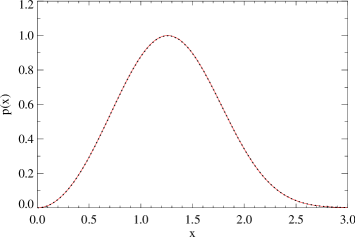
Figure 1.— A test of Algorithm. 3 for a PDF with $\sigma=x^{2}$. The red solid and black dotted lines are plotted according to the function $p(x)$ and sampling results obtained by Algorithm. 3, respectively.

2.4.2 the Scattering Transport

Now we discuss the momentum transport caused by the scattering kernel $C(\nu^{\prime}\rightarrow\nu,\mathbf{\Omega}^{\prime}\rightarrow\mathbf{\Omega}|\mathbf{r})$ (Eq. (6)). We first point out that the scattering kernel $C$ equals to the normalized scattering coefficient $\sigma_{s}$, which is related with the medium properties and also the different scattering mechanisms (or scattering cross sections). For example, in an uniform and isotropic medium, the scattering mechanism is Rayleigh scattering, then the scattering coefficient $\sigma_{s}$ is given by $n_{e}\sigma(\mathbf{\Omega}^{\prime}\rightarrow\mathbf{\Omega})$, where $n_{e}$ is the electron number density and $\sigma$ is the Rayleigh scattering cross section.

In the former discussions we took an implicit assumption that the scattering medium was static. This is an appropriate approximation for low energy or non-relativistic scattering medium, where the speed of the plasma can be neglected. While in more practical circumstances the effects induced by the motion or the velocity distribution of the scattering particles can not be ignored. In the simplest case, the velocities of the particles are isotropic and distribute according to the relativistic Maxwell distribution which is given by (Synge, 1957)

$$\begin{split}&\displaystyle N_{e}(\gamma,T_{e})=n_{e}\frac{v\gamma^{2}\exp(-\gamma/\Theta)}{\Theta K_{2}(1/\Theta)},\end{split}$$ (27)

where $\Theta=kT_{e}/m_{e}c^{2}$ is the dimensionless temperature of the gas, $\gamma$ is the Lorentz factor, and $K_{2}$ is the modified Bessel function of second kind of order two.

A photon with four momentum $\mathbf{p}=(E,\mathbf{\Omega})$ transporting in a hot electron gas will experience an averaged Compton scattering process, which can be described by a modified differential cross section. The quantities in this cross section are defined with respect to three different frames, i.e., the static frame whose basis vectors are $\mathbf{e}_{x},\,\mathbf{e}_{y},\,\mathbf{e}_{z}$, in which the incident and scattered directions are denoted by $\mathbf{\Omega}$ and $\mathbf{\Omega}^{\prime}$. The second frame is attached to $\mathbf{\Omega}$, whose basis vectors are $\mathbf{e}_{z}(p)=\mathbf{\Omega}$, $\mathbf{e}_{y}(p)=\mathbf{\Omega}\times\mathbf{e}_{z}/|\mathbf{\Omega}\times\mathbf{e}_{z}|$, $\mathbf{e}_{x}(p)=\mathbf{e}_{y}(p)\times\mathbf{e}_{z}(p)$ (see Fig. 2), in which the electron’s momentum vector $\mathbf{p}_{e}$ is defined and characterized by $(\gamma,\mu_{e},\phi_{e})$. The final frame is attached to $\mathbf{p}_{e}$, i.e., $\mathbf{e}_{z}(e)=\mathbf{p}_{e}$, $\mathbf{e}_{x}(e)=\mathbf{p}_{e}\times\mathbf{e}_{z}(p)/|\mathbf{p}_{e}\times\mathbf{e}_{z}(p)|$ and $\mathbf{e}_{y}(e)=\mathbf{e}_{z}(e)\times\mathbf{e}_{x}(e)$ (see Fig. 3). In this frame, the expression of Compton scattering differential cross section can be given appropriately. The incident and scattered directions are denoted by $(\mu_{e},\phi_{e})$ and $(\mu_{e}^{\prime},\phi_{e}^{\prime})$ respectively, and obviously we have $\phi_{e}\equiv-\pi/2$ (see Fig. 3). Any two of these frames are simply connected by an orthonormal transformation.

Then the scattering coefficient is given by the averaged Klein-Nishima (KN) differential cross section (Canfield et al., 1987), i.e.,

$$\begin{split}&\displaystyle\sigma_{s}(\nu\rightarrow\nu^{\prime},\mathbf{\Omega}\rightarrow\mathbf{\Omega}^{\prime})=\frac{1}{4\pi}\int_{1}^{\infty}d\gamma N_{e}(\gamma)\int_{-1}^{1}d\mu_{e}\\ &\times(1-\mu_{e}v)\int_{0}^{2\pi}d\phi_{e}\frac{d\sigma_{\text{KN}}}{d\mu_{e}^{\prime}d\phi_{e}^{\prime}}\delta\left[\nu^{\prime}-g(\nu,\mu_{e},\mu_{e}^{\prime},\psi)\right],\end{split}$$ (28)

where $d\sigma_{\text{KN}}/d\mu_{e}^{\prime}d\phi_{e}^{\prime}$ is the KN cross section (Akhiezer & Berestetskii, 1969)

$$\begin{split}&\displaystyle\frac{d\sigma_{\text{KN}}}{d\mu_{e}^{\prime}\phi_{e}^{\prime}}=\frac{3\sigma_{T}}{16\pi}\frac{1}{\gamma^{2}}\frac{\chi}{(1-\mu_{e}v)^{2}}\left(\frac{\nu^{\prime}}{\nu}\right)^{2},\end{split}$$ (29)

where

$$\begin{split}\left\{\begin{array}[]{ll}&\displaystyle\chi=\frac{\epsilon^{\prime}}{\epsilon}+\frac{\epsilon}{\epsilon^{\prime}}+\frac{4}{\epsilon}\left(1-\frac{\epsilon}{\epsilon^{\prime}}\right)+\frac{4}{\epsilon^{2}}\left(1-\frac{\epsilon}{\epsilon^{\prime}}\right)^{2};\\ &\displaystyle\epsilon=\frac{2h\nu}{m_{e}c^{2}}\gamma(1-\mu_{e}v),\quad\epsilon^{\prime}=\frac{2h\nu^{\prime}}{m_{e}c^{2}}\gamma(1-\mu_{e}^{\prime}v);\\ &\displaystyle g(\nu,\mu_{e},\mu_{e}^{\prime},\psi)=\frac{(1-\mu_{e}v)\nu}{1-\mu_{e}^{\prime}v+(h\nu/\gamma m_{e}c^{2})(1-\mu_{\psi})},\end{array}\right.\end{split}$$ (30)

where $\nu$ and $\nu^{\prime}$ are the incident and scattered frequencies respectively, $\psi$ is angle between the incident and scattered directions and $\mu_{\psi}=\cos\psi$. From Eq. (28) we can obtain the total scattering coefficient by integrating out all of the scattered directions $\mathbf{\Omega}^{\prime}$ and frequencies $\nu^{\prime}$ as

$$\begin{split}&\displaystyle\sigma_{s}(\nu,T_{e})=\int_{0}^{\infty}\int_{4\pi}\sigma_{s}(\nu\rightarrow\nu^{\prime},\mathbf{\Omega}\rightarrow\mathbf{\Omega}^{\prime})d\nu^{\prime}d\mathbf{\Omega}^{\prime}.\end{split}$$ (31)

Then the normalized scattering kernel is given by

$$\begin{split}&\displaystyle C(\nu\rightarrow\nu^{\prime},\mathbf{\Omega}\rightarrow\mathbf{\Omega}^{\prime})=\frac{\sigma_{s}(\nu\rightarrow\nu^{\prime},\mathbf{\Omega}\rightarrow\mathbf{\Omega}^{\prime})}{\sigma_{s}(\nu,T_{e})}.\end{split}$$ (32)

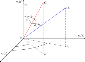
Figure 2.— The schematic demonstration of the tetrad ($\mathbf{e}_{i}(p)$, $i=x,y,z$) attached to the momentum direction $\mathbf{\Omega}$ of the incident photon. $\mathbf{\Omega}^{\prime}$ and $\mathbf{\Omega}_{e}$ represent the momentum directions of scattered photon and the scattering electron, respectively.

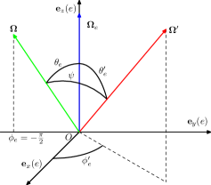
Figure 3.— The schematic demonstration of the tetrad ($\mathbf{e}_{i}(e)$, $i=x,y,z$) attached to the momentum direction $\mathbf{\Omega}_{e}$ of the scattering electron. $\mathbf{\Omega}$ and $\mathbf{\Omega}^{\prime}$ represent the momentum directions of incident and scattered photons, respectively.

The integral given by Eq. (31) can be computed either in the frame of $\mathbf{e}_{i}(p)$ or $\mathbf{e}_{i}(e)$. The components of $\mathbf{\Omega}^{\prime}$ in $\mathbf{e}_{i}(p)$ and $\mathbf{e}_{i}(e)$ are given by $(\psi,\phi^{\prime})$ and $(\theta^{\prime}_{e},\phi^{\prime}_{e})$ respectively. Then from the geometrical relationships depicted in Figure. 2 and 3, we have

$$\begin{split}\left\{\begin{array}[]{ll}&\displaystyle\mu_{e}^{\prime}=\mu_{\psi}\mu_{e}+\sqrt{1-\mu_{\psi}^{2}}\sqrt{1-\mu_{e}^{2}}\cos(\phi_{e}-\phi^{\prime}),\\ &\displaystyle\mu_{\psi}=\mu_{e}\mu_{e}^{\prime}+\sqrt{1-\mu_{e}^{2}}\sqrt{1-\mu_{e}^{\prime 2}}\cos\phi_{e}^{\prime}.\end{array}\right.\end{split}$$ (33)

From those we can obtain the Jacobian of the transformation given by

$$\begin{split}&\displaystyle J=\left|\begin{array}[]{ll}\displaystyle\frac{\partial(\mu_{\psi},\phi)}{\partial(\mu_{e}^{\prime},\phi_{e}^{\prime})}\end{array}\right|=1,\end{split}$$ (34)

hence the integral of $\mathbf{\Omega}^{\prime}$ amounts to $\displaystyle\int\frac{d\sigma_{\text{KN}}}{d\mu_{e}^{\prime}d\phi_{e}^{\prime}}d\mu_{e}^{\prime}d\phi_{e}^{\prime}$, which gives

$$\begin{split}&\displaystyle\sigma_{\text{KN}}(\epsilon)=\frac{3\sigma_{T}}{4}\frac{1}{\epsilon}\left[\left(1-\frac{4}{\epsilon}-\frac{8}{\epsilon^{2}}\right)\ln(1+\epsilon)+\frac{1}{2}\right.\\ &\left.+\frac{8}{\epsilon}-\frac{1}{2(1+\epsilon)^{2}}\right],\end{split}$$ (35)

then we have (Canfield et al., 1987)

$$\begin{split}&\displaystyle\sigma_{s}(\nu,T_{e})=\frac{1}{2}\int_{1}^{\infty}d\gamma\int_{-1}^{1}d\mu_{e}(1-\mu_{e}v)N_{e}(\gamma)\sigma_{\text{KN}}(\epsilon),\end{split}$$ (36)

where the integral of $d\phi_{e}$ has been finished trivially since $\sigma_{\text{KN}}(\epsilon)$ is independent on $\phi_{e}$. For its frequent request we can tabulate the values of $\sigma_{a}(\nu,T_{e})$ in terms of a properly divided grid of $\nu$ and $T_{e}$, and evaluate the value of $\sigma_{a}(\nu,T_{e})$ through the linear interpolation (Hua, 1997). There are also some other schemes to evaluate $\sigma_{a}(\nu,T_{e})$ numerically (Wienke, 1985).

Now we need to sample a scattered photon from $C$ (eq. (32)) with given incident $\nu$ and $\mathbf{\Omega}$. While $C$ involves a multiple integral in terms of the distribution function of hot electron gas. To illustrate the structure of $C$ in a more succinct form, we recast it as

$$\begin{split}&\displaystyle C(P^{\prime})=\int f(P^{\prime}|P_{e})f_{e}(P_{e})dP_{e},\end{split}$$ (37)

where $P^{\prime}=(\nu^{\prime},\mathbf{\Omega}^{\prime})$, $\displaystyle f(P^{\prime}|P_{e})=d\sigma_{\text{KN}}/d\Omega^{\prime}/\sigma_{\text{KN}}(\epsilon)$, $f_{e}(P_{e})=N_{e}(\gamma)(1-\mu_{e}v)\sigma_{\text{KN}}(\epsilon)/\sigma_{s}(\nu,T_{e})$ and $P_{e}=(\gamma,\mu_{e},\phi_{e})$. Both $f$ and $f_{e}$ have been normalized with factors $\sigma_{\text{KN}}(\epsilon)$ and $\sigma_{s}(\nu,T_{e})$, thus they can be taken as PDFs for sampling. An algorithm called as composition sampling has been proposed by Kahn (1954) to deal with PDFs given with an integral. The algorithm simply reads

$$\begin{array}[]{ll}\text{①}&\text{Get a sample }Y_{e}\text{ for $P_{e}$ by sampling }f_{e}(P_{e});\\ \text{②}&\text{Substitute $Y_{e}$ back into $f(P^{\prime}|P_{e})$ and sample }\\ &f(P^{\prime}|Y_{e})\text{ to get a sample $X$ for $P^{\prime}$}.\end{array}$$

One can readily show that $X$ is a sample of $C(P^{\prime})$. The sampling of $f_{e}(P_{e})$ is usually called as selecting an electron to scatter off the photon. The algorithms to sample $f_{e}(P_{e})$ have already been proposed and here we adopt a combined one consisting of that proposed by Canfield et al. (1987) and by Hua (1997) respectively. Since the former one involves an acceptation probability that equals to the ratio of $\sigma_{\text{KN}}$ to the Thomson cross sections $\sigma_{T}$, which becomes quite low for high energy photon scattering due to KN effect. While this drawback can be overcome by the algorithm proposed by Hua (1997) properly.

The sampling of $f(P^{\prime}|Y_{e})$ is more subtle than that of $f_{e}(P_{e})$. Before the scattering, all relevant quantities should be transformed into the electron rest frame, where the formula of scattering cross section is greatly simplified. After the scattering, they need to be transformed back into the static frame again.

Here we try to understand this sampling procedure mathematically from the so-called transformation sampling method. The relevant formulae are useful in our estimation scheme. We demonstrate it through an example where the PDF $f(u,v)$ has two random variables, $u$ and $v$. Through a bijection transformation: $u=\varphi_{1}(x,y),v=\varphi_{2}(x,y)$, we can obtain the PDF for two new random variable $x$ and $y$ as $g(x,y)=f[\varphi_{1}(x,y),\varphi_{2}(x,y)]J$, where $J=|\partial(u,v)/\partial(x,y)|$ is the Jacobian of the transformation. Hopefully $g(x,y)$ can be simplified and readily sampled. Once the samples of $x,y$: $x_{i},y_{j}$ are obtained, the corresponding samples of $u,v$ are immediately given by $u=\varphi_{1}(x_{i},y_{j}),v=\varphi_{2}(x_{i},y_{j})$. Notice that the inverse CFD method is actually a special case of transformation sampling method, where the transformed PDF is uniformly distributed.

Now the Lorentz transformation sampling procedure for $f(P^{\prime}|Y_{e})$ is easily understandable. The expression of $f(P^{\prime}|Y_{e})$ given by Eq. (29) is a complicated function of $\mu_{e}^{\prime}$ and $\phi_{e}^{\prime}$. Fortunately there is a transformation in terms of two new variables, $\Psi$ and $\Phi$ given by

$$\begin{split}\left\{\begin{array}[]{ll}&\displaystyle\mu_{\Psi}=\widetilde{\mu}_{e}\widetilde{\mu}_{e}^{\prime}-\sqrt{1-\widetilde{\mu}_{e}^{\prime 2}}\sqrt{1-\widetilde{\mu}_{e}^{2}}\cos(\phi_{e}-\phi_{e}^{\prime}),\\ &\displaystyle\cos\Phi=\frac{\widetilde{\mu}_{e}^{\prime}-\mu_{\Psi}\widetilde{\mu}_{e}}{\sqrt{1-\widetilde{\mu}_{\Psi}^{2}}\sqrt{1-\widetilde{\mu}_{e}^{2}}},\end{array}\right.\end{split}$$ (38)

where $\mu_{\Psi}=\cos\Psi$, and

$$\begin{split}&\displaystyle\widetilde{\mu}_{e}=\frac{\mu_{e}-v}{1-\mu_{e}v},\quad\widetilde{\mu}_{e}^{\prime}=\frac{\mu_{e}^{\prime}-v}{1-\mu_{e}^{\prime}v}.\end{split}$$ (39)

Obviously, $\Psi$ and $\Phi$ are the azimuth angles of the scattered direction defined with respect to the incident direction of the photon in the rest frame of the electron. After some tedious calculations, one can obtain the Jacobian of this transformation as

$$\begin{split}&\displaystyle J=\left|\frac{\partial(\mu_{\Psi},\Phi)}{\partial(\mu_{e}^{\prime},\phi_{e}^{\prime})}\right|=\frac{1}{\gamma^{2}(1-\mu_{e}^{\prime}v)^{2}}.\end{split}$$ (40)

And the quantity $\epsilon^{\prime}/\epsilon$ becomes

$$\begin{split}&\displaystyle\frac{\epsilon^{\prime}}{\epsilon}=\frac{1}{1+\displaystyle\epsilon/2(1-\mu_{\Psi})}.\end{split}$$ (41)

Then the PDF in terms of $\mu_{\Psi}$ and $\Phi$ reads

$$\begin{split}&\displaystyle f(\mu_{\Psi},\Phi|Y_{e})=\frac{r_{e}^{2}}{2}\left(\frac{\epsilon^{\prime}}{\epsilon}\right)^{2}\left(\frac{\epsilon^{\prime}}{\epsilon}+\frac{\epsilon}{\epsilon^{\prime}}-\sin^{2}\Psi\right),\end{split}$$ (42)

which is exactly the differential cross section of Compton scattering. The sampling procedure for this simplified PDF will be easier and we will adopt the one provided by Hua (1997). Once we obtain $\Psi$ and $\Phi$, $\mu_{e}^{\prime},\phi_{e}^{\prime}$ can also be obtained immediately through the inverse transformation given by Eq. (38) and (39), which is the Lorentz transformation obviously.

In our estimation scheme, we need to evaluate the scattering kernel $C$ (given by Eqs. (32) or (37)) with $\mathbf{\Omega}^{\prime}(=\mathbf{\Omega}_{\text{obs}})$, $\nu$ and $\mathbf{\Omega}$ are specified and take it as a weight. One can see that with these quantities are given, the remaining thing is to calculate the integral in terms of $P_{e}$, which can be accomplished by the MC method, i.e., we obtain a set of values of $Y_{e}=(\gamma,\mu_{e},\phi_{e})$ by sampling $f(P_{e})$ and then take $f(P^{\prime}|Y_{e})=d\sigma_{\text{KN}}/d\Omega^{\prime}/\sigma_{\text{KN}}(\epsilon)$ as weight. And $f(P^{\prime}|Y_{e})$ can be computed either by Eq. (29) directly or by $f(\mu_{\Psi},\Phi|Y_{e})J$.

In this section we mainly discussed the sampling procedure for the unpolarized Compton scattering with hot electron gas. The procedure for the polarized Compton and Rayleigh scattering with Stokes parameters involved will be presented later.

2.5. the estimation of observable quantities

Now we will discuss how to calculate the observational quantities at infinity by using the weight functions, especially how to deal with the case where a $\delta$ function appears in the recording function. These quantities include energy spectrum, light curve, angular-dependent photon number flux, etc.. Basically we divide the energy (or any other variables) section, on which the spectra are distributed, into a set of bins. Then we count and accumulate the contributions made by each component of the random sequence according to which bin they belong to.

As we mentioned that the final observed quantities can not be constructed from radiative flux $\psi(\mathbf{r},\mathbf{\Omega},\nu)$ directly, since they are confined in the radiative region where the emission and scattering processes are fulfilled. However, $\psi$ absolutely plays a relevant role in the construction. The quantity received by the observer can be expressed as an integral of $\psi$ and recording function $f(P)$ (see Eq. (12)) given by Eqs. (14) and (15). Thus the problem is reduced to evaluate all of $I_{m}$. Since a random sequence of states $P_{1},\cdots,P_{N}$ is generated, we can immediately get the estimations $F_{m}$, given by Eq. (23), for any $I_{m}$ with $m\leq N$. We then accumulate the $F_{m}$ to the bin where the frequency $\nu_{m}$ belongs to and the magnitude of the spectrum in the $i$-th bin is given by

$$\begin{split}&F_{i}=\displaystyle\sum_{j}I_{m}^{j}(\nu_{i}),\end{split}$$ (43)

where superscript $j$ is used to indicate the contributions made by different components that may come from a same random sequence or different ones.

The strategy discussed here can be called as term by term estimation, since each term of the random sequence can make the contribution to the observational quantities (even though it may be rejected). Comparing to the photon tracing scheme, this strategy has a lower variance. While for each $I_{m}$ we need to compute an additional quantity $\exp[-\tau(\mathbf{r}_{m})]$, where $\tau(\mathbf{r}_{m})$ is the total optical depth and

$$\begin{split}&\displaystyle\tau(\mathbf{r}_{m})=\int_{0}^{s_{\text{max}}}\sigma(\mathbf{\Omega}_{m},\mathbf{r}_{m}+t\mathbf{\Omega}_{m},\nu_{m})dt,\end{split}$$ (44)

where $s_{\text{max}}$ is the distance along $\mathbf{\Omega}_{m}$ from $\mathbf{r}_{m}$ to the boundary surface of the radiative region. In the photon tracing scheme, a different estimation function is chosen and the calculation of $\exp[-\tau(\mathbf{r}_{m})]$ is actually replaced by the position transport samplings. It can be called as the final event estimation scheme and will be discussed in the next subsection.

Obviously if $\mathbf{\Omega}_{m}=\mathbf{\Omega}_{\text{obs}}$, we record the contribution of $I_{m}$, otherwise it will be rejected. This fact is appropriately described by the $\delta$ function in the recording function. Since $\mathbf{\Omega}_{m}$ in a random sequence are totally stochastic and unexpected, hence almost all of them will be rejected. This drawback however can be overcome naively in our scheme, i.e., we eliminate the $\delta$ function by integrating it out directly. After that integration the integral of $I_{m}$ becomes

$$\begin{split}\displaystyle I_{m}=&\int_{P_{1}}\cdots\int_{P_{m}}S(P_{1})K(P_{1}\rightarrow P_{2})\cdots K(P_{m}\rightarrow\mathbf{r},\nu,\mathbf{\Omega}_{\text{obs}})\\ &\times\exp[-\tau(\mathbf{r},\nu,\mathbf{\Omega}_{\text{obs}})]dP_{1}\cdots dP_{m}d\mathbf{r}d\nu.\end{split}$$ (45)

Then we can choose a new recording function given by

$$\begin{split}&\displaystyle f_{\text{new}}=C(\nu_{m},\mathbf{\Omega}_{m}\rightarrow\nu,\mathbf{\Omega}_{\text{obs}})\cdot\exp[-\tau(\mathbf{r}_{m+1},\nu,\mathbf{\Omega}_{\text{obs}})],\end{split}$$ (46)

where the scattering kernel $C$ is completely determined since $\nu$ is fixed as the incident $\nu_{m},\mathbf{\Omega}_{m}$ and scattered direction $\mathbf{\Omega}_{\text{obs}}$ are specified. Also notice that for Compton scattering with averaged cross section, there is an extra weight factor, $\sigma_{s}(\nu_{m},T_{e})$, needs to be included. It arises from the procedure of sampling the electron distribution function $f(P_{e})$. Then the estimation function for $I_{m}$ given by Eq. (23) becomes

$$\begin{split}&\displaystyle F=w_{s,1}\cdot w_{s,2}\cdots w_{s,m}\cdot f_{\text{new}}.\end{split}$$ (47)

With this strategy, one can see that any term of a random sequence can always make contributions to the observational quantities. This can significantly improve the calculation efficiency and accuracy. And this strategy is very natural from the perspective of integral evaluation, since the value of a $\delta$ function involved integral can be obtained directly, i.e., $\int_{a}^{b}f(x)\delta(x-x_{0})dx=f(x_{0})$. This is absolutely one of the most important advantages to build the MCRT based on of Neumann solution.

Particularly, in the calculation of the angular dependent spectrum, we can obtain the values corresponding to all poloidal angles $\theta_{i}$ simultaneously, i.e., we evaluate $f_{\text{new}}$ for $n$ times with different $\mu_{i}=\cos\theta_{i}$. This procedure can genuinely increase the computational efficiency and accuracy (see the discussions in the section of scheme verification).

2.6. final event estimation

Now we discuss how to understand the photon tracing scheme from the perspective of Neumann solution and demonstrate that it actually corresponds to a special choice of estimation function, i.e., the final event estimation. Where a photon (or superphoton) is generated and traced until to its ending, either escaping from the radiative region, or absorbed by the medium. These steps can be derived from the estimation function.

Physically speaking both the absorption and scattering coefficients $\sigma_{a}$ and $\sigma_{s}$ vanish outside the radiative domain, which implies that the photons actually can never escape from the region, since $p(s)=\exp[-\int_{0}^{s}\sigma_{s}(t)dt]\sigma_{s}(s)/A\equiv 0$, if $s>s_{b}$. But mathematically we have the flexibility to choose an arbitrary function as PDF, provided its corresponding weight can give a correct unbiased estimation for the final result. Thus we extend the definition zone of $\sigma_{s}$ to the whole space by filling the outer vacuum with an auxiliary medium, and in which $\sigma_{s}$ can be an arbitrary function, provided $\tau_{s}(s)$ blows up as $s$ approaches infinity, i.e., $\lim\limits_{s\rightarrow\infty}\tau_{s}(s)\rightarrow\infty$. With $\sigma_{s}$, both the scattering optical depth $\tau_{s}(s)$ and $p(s)$ are non-vanishing in the whole position space. The form of $p(s)$ now becomes $p(s)ds=\exp(-\tau_{s})d\tau_{s}$ and $A=1$. We use $p(s)$ to sample the scattering distance $s$ and the photon has the probability to escape from the radiative region. Then one can readily show the following identity as

$$\begin{split}\exp[-\tau_{s}(s_{b})]=\int^{\infty}_{0}H(s^{\prime}-s_{b})p(s^{\prime})ds^{\prime},\end{split}$$ (48)

where $H(s^{\prime}-s_{b})$ is the Heaviside function. With that the recording function $f(P)$ can be rewritten as

$$\begin{split}f(P)=&\delta(\mathbf{\Omega}-\mathbf{\Omega}_{\text{obs}})\exp[-\tau_{a}(s_{b})]\\ &\times\int^{\infty}_{0}H(s^{\prime}-s_{b})p(s^{\prime})ds^{\prime},\end{split}$$ (49)

where $\tau_{a}(s_{b})$ is the absorption optical depth. Substituting $f(P)$ into Eq. (15), we can reselect the associated PDF and estimation function respectively as

$$\begin{split}&\displaystyle\widetilde{f}(P1,\cdots,P_{m},P)=S(P_{1})\cdot T_{s}(\mathbf{r}_{1}\rightarrow\mathbf{r}_{2})\cdot C(\nu_{1},\mathbf{\Omega}_{1}\rightarrow\\ &\nu_{2},\mathbf{\Omega}_{2})\cdots T_{s}(\mathbf{r}_{m}\rightarrow\mathbf{r})\cdot C(\nu_{m},\mathbf{\Omega}_{m}\rightarrow\nu,\mathbf{\Omega})\cdot T_{s}(\mathbf{r}\rightarrow\mathbf{r}^{\prime}),\end{split}$$ (50)

$$\begin{split}\displaystyle F=&w_{s,1}\cdot w_{s,2}\cdots w_{s,m}\cdot f_{\text{new}},\end{split}$$ (51)

where $T_{s}=\exp(-\tau_{s})d\tau_{s}$, $w_{s,i}=\exp(-\tau_{a})$, $\mathbf{r}^{\prime}=\mathbf{r}+s^{\prime}\mathbf{\Omega}$ and

$$\begin{split}f_{\text{new}}=&\delta(\mathbf{\Omega}-\mathbf{\Omega}_{\text{obs}})\exp[-\tau_{a}(s_{b})]H(s^{\prime}-s_{b}).\end{split}$$ (52)

Due to the factor $H(s^{\prime}-s_{b})$, $F$ always vanishes and the corresponding contribution is rejected, unless the scattering distance $s>s_{b}$. And $s>s_{b}$ means that the photon has escaped the radiative region. This is what the final event estimation means. While from Eq. (48) one can can see that the final event estimation is nothing but evaluating the factor $\exp[-\tau_{s}(s_{b})]$ by sampling $p(s)$ and taking $H(s_{i}-s_{b})$ as weight, where $s_{i}$ are the samples of $s$, and

$$\begin{split}\displaystyle\exp[-\tau_{s}(s_{b})]\approx\sum_{i=1}^{N}H(s_{i}-s_{b})=\frac{M}{N},\end{split}$$

where $N$ is the number of samples and $M$ is the number of $s_{i}$ greater than $s_{b}$.

Compared to the term by term estimation, the final event estimation has been applied more widely in the former RT researches (e.g., Dolence et al. (2009), Schnittman & Krolik (2013), etc.). However there are also some shortages for the final event estimation. For example its variance is higher than term by term estimation, since for any sequence there is only one chance to record the contribution. Especially in an optically thin system, where the photons are prone to escape rather than scattering. To overcome this difficulty, Dolence et al. (2009) adopted a biased PDF for position transport sampling, i.e., $p(s)=\exp(-b\tau_{s})d(b\tau_{s})$, where $b$ is called as bias parameter, by tuning the its value one can implement the sampling process in a better way and improve the poor signal to noise performance. Obviously an additional weight $w_{b}=\exp[-\tau_{s}(1-b)]/b$ is needed to balance the biased sampling.

While in the term by term estimation scheme, such problem will not plagues us anymore, since the radiation sampling is mandatorily confined in the radiative region. This is a variation of the weighted sampling technique discussed by Pozdnyakov et al. (1983). The low optical depth exerts its effect on the term by term estimation scheme through the normalization factor $A=1-\exp(-\tau_{s})\approx\tau_{s}$. Thus the contributions made by the sufficiently scattered radiations will diminish rapidly.

3. the polarized radiative transfer

In the above section we have demonstrated how to solve an RTE systematically by evaluating the multiple integrals stem from its Neumann solution, where we ignored the polarization effects. The purpose of this section is to include these effects by extending the scheme. The treatment of polarized RT surely becomes more complicated. However taking the former discussion as a foundation, we can also treat the polarized RT in a consistent way, where the Neumann solution also plays a significant role.

The polarizations of radiation are appropriately described by the Stokes parameters of $I,Q,U,V$ (Chandrasekhar, 1960) and the polarized RTE becomes a set of integro-differential equations on these parameters. Similarly, by introducing four auxiliary quantities (called as radiation flux), these equations can be transformed into a set of integral equations. Then their Neumann solutions are naturally obtained and observational quantities can be evaluated directly by these solutions.

3.1. the Stokes Parameters

To describe polarization, we must introduce the Stokes parameters (SPs) of $I,Q,U,V$, where $I$ is the radiation intensity, $Q,U$ and $V$ depict the linear and circular polarizations, respectively. It is convenient to group them as a column vector, i.e., $\mathbf{I}=(I,Q,U,V)^{T}$. The components $Q$ and $U$ are defined with respect to a reference in the plane that is perpendicular to the direction of propagation. If the frame is rotated by an angle $\Phi$ anticlockwise in that plane, the SPs will change as

$$\begin{split}&\displaystyle\mathbf{I}^{\prime}=\mathbf{M}(\Phi)\mathbf{I},\end{split}$$ (53)

where

$$\mathbf{M}(\Phi)=\left(\begin{array}[]{cccc}1&0&0&0\\ 0&\quad\cos 2\Phi&\sin 2\Phi&0\\ 0&-\sin 2\Phi&\cos 2\Phi&0\\ 0&0&0&1\end{array}\right).$$ (54)

A vector used to fix a frame in the transverse plane is called as polarization vector. In order to determine the SPs at any position, we need to parallel transport the polarization vector along the ray trajectory and trace their changes after any scattering as well. In flat spacetime, the parallel transport of a vector along a straight line is trivial and the vector remains unchanged. In scattering process, the scattering matrix is implicitly defined with respect to the scattering plane, which is determined by the incident and scattered directions of the photon. In the description of RT of Chandrasekhar (1960), the polarization vector was always defined in a meridian plane that was determined by the wave vector $\mathbf{k}$ and the base vector $\mathbf{e}_{z}$ of the static reference. Thus the SPs experienced two rotation transformations just before and after any scattering process respectively (see Eq. (71)).

For Rayleigh scattering, the scattering matrix $\mathbf{R}$ defined with respect to the scattering plane is given by (Chandrasekhar, 1960)

$$\begin{split}&\mathbf{R}=\frac{3}{16\pi}\delta(\nu-\nu^{\prime})\times\\ &\times\left(\begin{array}[]{cccc}1+\cos^{2}\Theta&-\sin^{2}\Theta&0&0\\ -\sin^{2}\Theta&1+\cos^{2}\Theta&0&0\\ 0&0&2\cos\Theta&0\\ 0&0&0&2\cos\Theta\end{array}\right),\end{split}$$ (55)

where $\Theta$ is the scattering angle.

The description of polarized photon scattered by unpolarized electron is more complicated (Nagirner & Poutanen, 1993; Poutanen & Vilhu, 1993). The polarization vector of a photon is actually the spin wave function $\Ket{\mathbf{e}}$, which can be expressed as the sum of two base states: $\Ket{\mathbf{e}}=c_{x}\Ket{\mathbf{e}_{x}}+c_{y}\Ket{\mathbf{e}_{y}}$, where $\Ket{\mathbf{e}_{x}}$ and $\Ket{\mathbf{e}_{y}}$ can either be linear or (left and right) circular polarization states respectively. $c_{x}$ and $c_{y}$ are two complex numbers and their squared absolute values are the probabilities that the photon is found in the corresponding states. We can further introduce the density matrix defined as: $\rho_{xy}=c_{x}c_{y}^{*}=\Braket{\mathbf{e}_{x}}{\mathbf{e}}\Braket{\mathbf{e}}{\mathbf{e}_{y}}$. Using Pauli matrices $\sigma_{i}$, $\rho_{xy}$ can be expressed as $\rho=\frac{1}{2}(I+\xi_{1}\sigma_{1}+\xi_{2}\sigma_{2}+\xi_{3}\sigma_{3})$, where $I$ is the unit matrix. $\xi_{i}$ are the SPs of a photon given by (Kosowsky, 1996)

$$\begin{split}&\xi_{1}=c_{x}c_{y}^{*}+c_{x}^{*}c_{y},\\ &\xi_{2}=i(c_{x}c_{y}^{*}-c_{x}^{*}c_{y}),\\ &\xi_{3}=|c_{x}|^{2}-|c_{y}|^{2},\end{split}$$ (56)

which are connected with the normalized SPs, i.e., $\xi_{1}=U/I,\xi_{2}=V/I,\xi_{3}=Q/I$. If we do a measurement, then the probability that we find the photon stays in the $\Ket{\mathbf{e}^{\prime}}$ state (the corresponding SPs are $\xi_{i}^{\prime}$) is given by

$$\begin{split}p=|\Braket{\mathbf{e}}{\mathbf{e}^{\prime}}|^{2}=\frac{1}{2}(1+\xi_{1}\xi_{1}^{\prime}+\xi_{2}\xi_{2}^{\prime}+\xi_{3}\xi_{3}^{\prime}).\end{split}$$ (57)

Suppose a polarized photon with $\xi_{i}$ is scattered by an unpolarized and static electron into a polarization state with $\xi_{i}^{(f)}$ in direction $(\mu,\varphi)$, then the probability (or the differential KN cross section) that a detector finds the scattered photon in the polarized state with $\xi_{i}^{\prime}$ is given by (Fano, 1949):

$$\begin{split}&\displaystyle d\sigma=\frac{r_{e}^{2}}{4}\left(\frac{\epsilon^{\prime}}{\epsilon}\right)^{2}[F_{0}+F_{3}\widetilde{\xi_{3}}+F_{11}\widetilde{\xi}_{1}\xi_{1}^{\prime}+F_{22}\xi_{2}\xi_{2}^{\prime}\\ &+(F_{33}\widetilde{\xi_{3}}+F_{3})\xi_{3}^{\prime}]d\mu d\varphi,\end{split}$$ (58)

where $\epsilon$ and $\epsilon^{\prime}$ are the energies of incident and scattered photons, $r_{e}$ is the classic electron radius, and the other parameters are given by (Fano, 1949, 1957)

$$\begin{array}[]{ll}&\displaystyle F_{0}=\frac{\epsilon^{\prime}}{\epsilon}+\frac{\epsilon}{\epsilon^{\prime}}-\sin^{2}\vartheta,\quad F_{3}=\sin^{2}\vartheta,\quad F_{11}=2\cos\vartheta\\ &\displaystyle F_{22}=\left(\frac{\epsilon^{\prime}}{\epsilon}+\frac{\epsilon}{\epsilon^{\prime}}\right)\cos\vartheta,\quad F_{33}=1+\cos^{2}\vartheta,\end{array}$$ (61)

and

$$\begin{split}&\displaystyle\widetilde{\xi_{3}}=-(\xi_{3}\cos 2\varphi+\xi_{1}\sin 2\varphi),\\ &\widetilde{\xi_{1}}=-(-\xi_{3}\sin 2\varphi+\xi_{1}\cos 2\varphi).\end{split}$$ (62)

Performing a summation over all possible polarized states with $\xi_{i}^{\prime}$ in the direction $(\mu,\varphi)$ , we obtain the total KN cross section as

$$\begin{array}[]{ll}d\sigma&\displaystyle=\frac{r_{e}^{2}}{2}\left(\frac{\epsilon^{\prime}}{\epsilon}\right)^{2}(F_{0}+F_{3}\widetilde{\xi_{3}})d\mu d\varphi.\end{array}$$ (64)

Comparing the coefficients before $\xi_{i}^{\prime}$ in Eqs. (57) and (58), we have

$$\left\{\begin{array}[]{ll}&\displaystyle\xi^{(f)}_{1}=\frac{F_{11}\widetilde{\xi_{1}}}{F_{0}+F_{3}\widetilde{\xi_{3}}},\\ &\displaystyle\xi^{(f)}_{2}=\frac{F_{22}\xi_{2}}{F_{0}+F_{3}\widetilde{\xi_{3}}},\\ &\displaystyle\xi^{(f)}_{3}=\frac{F_{3}+F_{33}\widetilde{\xi_{3}}}{F_{0}+F_{3}\widetilde{\xi_{3}}}.\end{array}\right.$$ (68)

Combining the above equations and the relations between $\xi_{i}$ and $(I,Q,U,V)$, we can obtain the transformation formula for incident and scattered SPs as (Mościbrodzka, 2020)

$$\begin{pmatrix}I^{\prime}\\ Q^{\prime}\\ U^{\prime}\\ V^{\prime}\end{pmatrix}=\left(\frac{\epsilon^{\prime}}{\epsilon}\right)^{2}\begin{pmatrix}F_{0}&F_{3}&0&0\\ F_{3}&F_{33}&0&0\\ 0&0&F_{11}&0\\ 0&0&0&F_{22}\end{pmatrix}\begin{pmatrix}\widetilde{I}\\ \widetilde{Q}\\ \widetilde{U}\\ \widetilde{V}\end{pmatrix},$$ (69)

where $\widetilde{\mathbf{I}}=\mathbf{M}(\varphi)\mathbf{I}$. One may notice that the above formulae are valid just in the rest frame of the electron. However the corresponding formulae in an arbitrary frame can easily be obtained through a Lorentz transformation. Utilizing the Jacobian of a Lorentz transformation given by Eq. (40), we have

$$\mathbf{I}^{\prime}=\frac{1}{\gamma^{2}(1-\mu_{e}v)^{2}}\left(\frac{\nu^{\prime}}{\nu}\right)^{2}\mathbf{F}\mathbf{M}(\varphi)\mathbf{I},$$ (70)

which is very useful in our scheme for polarized Compton scattering, i.e., as the scattered direction is replaced by $\mathbf{\Omega}_{\text{obs}}$, the results on the RHS will be used as weights for observed SPs. Krawczynski (2012) gave a systematical but complicated discussions on the transformation procedures for such scattering, especially the transformations and rotations for SPs. In our scheme, the corresponding treatment can be somehow simplified greatly.

3.2. the Neumann Solution for Polarized RTEs

Now we begin to demonstrate how to solve the polarized RTEs by the method based upon the Neumann solution as discussed before. We will take the polarized RTEs of Chandrasekhar (1960) in flat spacetime as an example. These equations were first appropriately formulated by Chandrasekhar (1960) (also see Pomraning (1973) for a more pedagogical introduction), in which the Faraday rotation and conversion effects were not taken into consideration. So the total absorption coefficient matrix will take the form of $\sigma(\nu)E$, where $E$ is the unit matrix, $\sigma(\nu)$ is the total interaction coefficient. The polarized RTEs with scattering process incorporated read (Pomraning, 1973)

$$\begin{split}&\displaystyle\mathbf{\Omega}\cdot\nabla\mathbf{I}(\nu,\mathbf{\Omega},\mathbf{r})+\sigma(\nu,\mathbf{\Omega},\mathbf{r})\mathbf{I}(\nu,\mathbf{\Omega},\mathbf{r})\\ &=\mathbf{S}(\nu,\mathbf{\Omega},\mathbf{r})\displaystyle+\int_{0}^{\infty}d\nu^{\prime}\int_{4\pi}d\mathbf{\Omega}^{\prime}\sigma_{s}(\nu^{\prime},\mathbf{\Omega}^{\prime},\mathbf{r})\frac{\nu}{\nu^{\prime}}\\ &\times\mathbf{M}(\pi-\psi)\mathbf{R}(\nu^{\prime}\rightarrow\nu,\cos\Theta)\mathbf{M}(\Phi)\mathbf{I}(\nu^{\prime},\mathbf{\Omega}^{\prime},\mathbf{r}),\end{split}$$ (71)

where $\cos\Theta=\mathbf{\Omega}\cdot\mathbf{\Omega}^{\prime}$ is the cosine of scattering angle, $\Phi$ is the angle between the incident meridian plane and the scattering plane, $\sigma(\nu)=\sigma_{a}(\nu)+\sigma_{s}(\nu)$, $\sigma_{a}(\nu)$ and $\sigma_{s}(\nu)$ are the absorption and scattering coefficients at frequency $\nu$, respectively. As aforementioned $\mathbf{I}=(I,Q,U,V)^{T}$ represents the SPs vector and $\mathbf{S}=(S_{I},S_{Q},S_{U},S_{V})^{T}$ represents the emissivity vector, whose components characterize the polarized radiations emitted by the medium spontaneously. Since we prefer to use $I,Q$ rather than $I_{l},I_{r}$ in MCRT, the scattering matrix $\mathbf{R}$ is different from that given by Chandrasekhar (1960) (see the discussion in Appendix C). Since the polarization vector always lies in the meridian plane and the scattering matrix $\mathbf{R}$ is defined with respect to the scattering plane, we need use the rotation matrix $\mathbf{M}(\Phi)$ to transform the SPs from the incident meridian plane to the scattering plane and the matrix $\mathbf{M}(\pi-\psi)$ to implement the inverse transformation. From the geometrical relations, one can easily show that $\psi$ is a function of $\Theta$ and $\Phi$. Thus we can simplify the expression of the scattering term by introducing a matrix $\mathbf{K}_{c}$ defined as $\mathbf{K}_{c}(\Theta,\Phi)=\mathbf{M}(\pi-\psi)\mathbf{R}(\cos\Theta)\mathbf{M}(\Phi)$.

On the other hand, we can recast the transfer equations with respect to the static frame, in which the incident and scattered directions of the radiation are denoted by $\theta^{\prime},\phi^{\prime}$ and $\theta,\phi$ respectively. One can show that $\Theta,\Phi$ are the triangular functions of $\theta,\phi$ with given $\theta^{\prime},\phi^{\prime}$ (Chandrasekhar, 1960), implying that $\mathbf{K}_{c}$ is also a function of $\theta,\phi$. Hence we can either use $\Theta,\Phi$ or $\theta,\phi$ to describe the scattering process. In our scheme we prefer to use $\theta,\phi$, even though the elements of matrix $\mathbf{K}_{c}$ are very complicated functions of them (see Appendix C). Because we need not consider any complicated rotations and transformations in terms of $\mathbf{M}(\Phi)$ and $\mathbf{M}(\pi-\psi)$ and the related tetrad constructions.

Now we can implement the similar procedures to transform the RTEs into a set of integral equations on an auxiliary quantity $\mathbf{\Psi}(\nu,\mathbf{\Omega},\mathbf{r})$, which exactly equals to the RHS of Eq. (71), i.e.,

$$\begin{split}&\displaystyle\mathbf{\Psi}(\nu,\mathbf{\Omega},\mathbf{r})=\mathbf{S}(\nu,\mathbf{\Omega},\mathbf{r})\displaystyle+\\ &\int_{0}^{\infty}d\nu^{\prime}\int_{4\pi}d\mathbf{\Omega}^{\prime}\sigma_{s}(\nu^{\prime},\mathbf{\Omega}^{\prime},\mathbf{r})\frac{\nu}{\nu^{\prime}}\mathbf{K}_{c}(\Theta,\Phi)\mathbf{I}(\nu^{\prime},\mathbf{\Omega}^{\prime},\mathbf{r}).\end{split}$$ (72)

Notice that the gradient derivative on the LHS of Eq. (71) can be recast into a total derivative with respect to the distance $s$ along the radiation, i.e.,

$$\begin{split}&\displaystyle-\frac{d}{ds}\mathbf{I}\left(\nu,\mathbf{\Omega},\mathbf{r}-s\mathbf{\Omega}\right)=\mathbf{\Omega}\cdot\nabla\mathbf{I}\left(\nu,\mathbf{\Omega},\mathbf{r}-s\mathbf{\Omega}\right).\end{split}$$ (73)

Then Eq. (71) becomes (see the page 27 of Pomraning (1973))

$$\begin{split}&\displaystyle-\frac{d}{ds}\mathbf{I}\left(\nu,\mathbf{\Omega},\mathbf{r}-s\mathbf{\Omega}\right)+\sigma\left(\nu,\mathbf{\Omega},\mathbf{r}-s\mathbf{\Omega}\right)\\ &\times\mathbf{I}\left(\nu,\mathbf{\Omega},\mathbf{r}-s\mathbf{\Omega}\right)=\mathbf{\Psi}\left(\nu,\mathbf{\Omega},\mathbf{r}-s\mathbf{\Omega},\right).\end{split}$$ (74)

Integrating the above equation formally, we have

$$\begin{split}&\displaystyle\mathbf{I}(\nu,\mathbf{\Omega},\mathbf{r})=\int_{0}^{|\mathbf{r}-\mathbf{r}_{0}|}ds^{\prime}\mathbf{\Psi}\left(\nu,\mathbf{\Omega},\mathbf{r}-s^{\prime}\mathbf{\Omega},\right)\\ &\times\exp\left[-\int^{s^{\prime}}_{0}\sigma\left(\nu,\mathbf{\Omega},\mathbf{r}-s^{\prime\prime}\mathbf{\Omega}\right)ds^{\prime\prime}\right],\end{split}$$ (75)

where $\mathbf{r}_{0}$ is the position vector of the starting point of the ray trajectory on the boundary. If the radiative region is infinite, we have $|\mathbf{r}-\mathbf{r}_{0}|=\infty$. We should keep in mind that $\mathbf{I}$ is a column vector with four components, thus the above equation means that the four components share a common exponential attenuation factor as the radiation propagates. For the RT in a magnetized plasma where the Faraday rotation and conversion effects should be considered (Shcherbakov & Huang, 2011; Huang & Shcherbakov, 2011), the absorption coefficient will be replaced by a matrix, which gives rise to the failure of the integration procedure of Eq. (74). However we can still employ it by introducing a $\sigma(\nu)I$ term and alter the coefficient matrix (see the discussion below).

Substituting Eq. (75) into the RHS of Eq. (72), we obtain the integral equation of $\mathbf{\Psi}$

$$\begin{split}&\displaystyle\mathbf{\Psi}(\nu,\mathbf{\Omega},\mathbf{r})=\mathbf{S}(\nu,\mathbf{\Omega},\mathbf{r})\displaystyle+\int_{0}^{\infty}d\nu^{\prime}\int_{4\pi}d\mathbf{\Omega}^{\prime}\int_{0}^{|\mathbf{r}-\mathbf{r}_{0}|}ds^{\prime}\\ &\times\sigma_{s}(\nu^{\prime},\mathbf{\Omega}^{\prime},\mathbf{r})\frac{\nu}{\nu^{\prime}}\mathbf{K}_{c}(\Theta,\Phi)\mathbf{\Psi}(\nu^{\prime},\mathbf{\Omega}^{\prime},\mathbf{r}_{0}+s^{\prime}\mathbf{\Omega})\\ &\times\exp\left[-\int^{|\mathbf{r}-\mathbf{r}_{0}|}_{s^{\prime}}\sigma\left(\nu^{\prime},\mathbf{\Omega}^{\prime},\mathbf{r}_{0}+s^{\prime\prime}\mathbf{\Omega}\right)ds^{\prime\prime}\right].\end{split}$$ (76)

Comparing to Eq. (75), we have reversed the direction of integration, i.e., from $\mathbf{r}_{0}$ to $\mathbf{r}$ for the sake of convenience. Denote $P=(\nu,\mathbf{\Omega},\mathbf{r})$, the above equation can be expressed in a compact form as

$$\begin{split}&\displaystyle\mathbf{\Psi}(P)=\mathbf{S}(P)\displaystyle+\int_{P^{\prime}}\mathbf{K}(P^{\prime}\rightarrow P)\mathbf{\Psi}(P^{\prime})dP^{\prime},\end{split}$$ (77)

where $\mathbf{K}(P^{\prime}\rightarrow P)=T_{s}\mathbf{C}w_{s}$ is the total transport kernel, $T_{s}$, $\mathbf{C}$ are the position transport and Compton scattering kernels respectively, $w_{s}$ is the weight factor for counting the effect of absorption, and

$$\begin{split}&\displaystyle T_{s}(\mathbf{r}_{s^{\prime}}\rightarrow\mathbf{r}|\nu^{\prime},\mathbf{\Omega}^{\prime})=\frac{1}{A}\sigma_{s}(\nu^{\prime},\mathbf{\Omega}^{\prime},\mathbf{r})\\ &\times\exp\left[-\int^{|\mathbf{r}-\mathbf{r}_{0}|}_{s^{\prime}}\sigma_{s}\left(\nu^{\prime},\mathbf{\Omega}^{\prime},\mathbf{r}_{0}+s^{\prime\prime}\mathbf{\Omega}\right)ds^{\prime\prime}\right],\\ &\mathbf{C}(\mathbf{\Omega}^{\prime}\rightarrow\mathbf{\Omega},\nu^{\prime}\rightarrow\nu|\mathbf{r})=\frac{\nu}{\nu^{\prime}}\mathbf{K}_{c}(\Theta,\Phi),\\ &w_{s}(s^{\prime})=A\exp\left[-\int^{|\mathbf{r}-\mathbf{r}_{0}|}_{s^{\prime}}\sigma_{\alpha}\left(\nu^{\prime},\mathbf{\Omega}^{\prime},\mathbf{r}_{0}+s^{\prime\prime}\mathbf{\Omega}\right)ds^{\prime\prime}\right],\end{split}$$ (78)

where $A$ is the normalization factor of $T_{s}$. Eq. (77) is a set of Fredholm integral equations of second kind and their Neumann series expansion can be directly obtained as

$$\begin{split}&\displaystyle\mathbf{\Psi}(P)=\sum_{m=0}^{\infty}\mathbf{\Psi}_{m}(P),\end{split}$$ (79)

where

$$\begin{split}\left\{\begin{array}[]{ll}&\displaystyle\mathbf{\Psi}_{0}(P)=\mathbf{S}(P),\\ &\displaystyle\mathbf{\Psi}_{1}(P)=\int\mathbf{K}(P_{0}\rightarrow P)\mathbf{\Psi}_{0}(P_{0})dP_{0}\\ &\displaystyle=\int\mathbf{K}(P_{0}\rightarrow P)\mathbf{S}(P_{0})dP_{0},\\ &\displaystyle\cdots,\\ &\displaystyle\mathbf{\Psi}_{m}(P)=\int\mathbf{K}(P_{m-1}\rightarrow P)\mathbf{\Psi}_{m-1}(P_{m-1})dP_{m-1}\\ &\displaystyle=\idotsint\displaystyle\mathbf{K}(P_{m-1}\rightarrow P)\cdots\mathbf{K}(P_{1}\rightarrow P_{2})\\ &\times\mathbf{K}(P_{0}\rightarrow P_{1})\mathbf{S}(P_{0})dP_{0}dP_{1}\cdots dP_{m-1}.\end{array}\right.\end{split}$$ (80)

Using Eq. (75), the SPs observed in the direction $\mathbf{\Omega}_{\text{obs}}$ can be expressed as an integral over the whole emissive region

$$\begin{split}\mathbf{I}&\displaystyle=\int_{P}\mathbf{\Psi}(P)f(P)dP=\sum_{m=0}^{\infty}\mathbf{I}_{m},\end{split}$$ (81)

where

$$\begin{split}\mathbf{I}_{m}&\displaystyle=\idotsint\displaystyle f(P)\mathbf{K}(P_{m-1}\rightarrow P)\cdots\mathbf{K}(P_{1}\rightarrow P_{2})\\ &\times\mathbf{K}(P_{0}\rightarrow P_{1})\mathbf{S}(P_{0})dP_{0}dP_{1}\cdots dP_{m-1}dP,\end{split}$$ (82)

and

$$\begin{split}&\displaystyle f(P)=\exp\left[-\int^{s_{b}}_{0}\sigma\left(\nu,\mathbf{\Omega},\mathbf{r}+s^{\prime\prime}\mathbf{\Omega}\right)ds^{\prime\prime}\right]\delta(\mathbf{\Omega}-\mathbf{\Omega}_{obs}).\end{split}$$ (83)

which is the recording function. Hence the problem of polarized RT can also be converted to the calculations of infinite multiple integrals arising from Neumann solution. Next we will demonstrate how to evaluate these integrals by the MC method.

3.3. the Generation of Random Sequence

Similarly to the unpolarized situations, in order to calculate the integrals given by Eq. (82) simultaneously, we need to generate a scattering sequence: $P_{0},P_{1},\cdots,$ by sampling an associated PDF separated from the integrand of $\mathbf{I}_{m}$. Meanwhile the remaining part is taken as weight functions for the estimation of $\mathbf{I}_{m}$. The kernel $\mathbf{K}(P^{\prime}\rightarrow P)$ is a matrix, which will mix the components of the column vector $\mathbf{\Psi}$ inevitably after its action on it, the evolution of them are coupled. Therefore we must appropriately find a PDF shared by the four components of $\mathbf{\Psi}$. For position transport, the four components share a common kernel: $T_{s}(\mathbf{r}_{s}\rightarrow\mathbf{r}|\nu,\mathbf{\Omega})$. While for scattering we have to choose a common PDF for all components. In addition, we define a weight variable $w$ and set its initial value to be $1$.

Our start point is also to generate $P_{0}$ by sampling the source function $\mathbf{S}(P)$. If $\mathbf{S}(P)$ is too complicated, we will sample an uniform PDF to get $P_{0}$ instead and take $\mathbf{S}(P_{0})$ as the weight for estimations, i.e., $\mathbf{\Psi}_{0}=\mathbf{S}(P_{0})$.

Next we need to generate $P_{m}$ when $P_{m-1}$ is provided by sampling the total transfer kernel $\mathbf{K}(P_{m-1}\rightarrow P_{m})$. Since $\mathbf{K}=T_{s}\mathbf{C}w_{s}$, we can use $T_{s}$ as the position transport PDF $p(s)$ for all components of $\mathbf{\Psi}$ and it can be sampled by using either inverse CDF method or the Algorithm. 3. With the distance sample $s$, we have $\mathbf{r}_{m}=\mathbf{r}_{m-1}+s\mathbf{\Omega}_{m-1}$. Accompanying each position transport, an extra weight $w_{s}$ (see Eq. (78)) must be multiplied to the weight: $w=w\cdot w_{s}$.

To obtain the PDF for scattering, we must carry out the multiplication of matrix $\mathbf{K}_{c}$ and $\mathbf{\Psi}_{m-1}$. After that, we get four updating relationships between the components of $\mathbf{\Psi}_{m-1}$ and $\mathbf{\Psi}_{m}$, i.e. ($\mathbf{\Omega}_{m}$ is determined by $\Theta_{m},\Phi_{m}$, for simplicity we will drop the subscript $m$ from now on),

$$\begin{split}\left\{\begin{array}[]{ll}&\displaystyle\Psi^{(I)}_{m}=f_{I}(\Theta,\Phi)\Psi^{(I)}_{m-1},\,\,\displaystyle\Psi^{(Q)}_{m}=f_{Q}(\Theta,\Phi)\Psi^{(I)}_{m-1},\\ &\displaystyle\Psi^{(U)}_{m}=f_{U}(\Theta,\Phi)\Psi^{(I)}_{m-1},\,\,\displaystyle\Psi^{(V)}_{m}=f_{V}(\Theta,\Phi)\Psi^{(V)}_{m-1},\end{array}\right.\end{split}$$ (84)

where

$$\begin{split}\left\{\begin{array}[]{ll}&\displaystyle f_{I}(\Theta,\Phi)=[1+\cos^{2}\Theta-\sin^{2}\Theta\times\\ &\quad\quad\quad\times(q_{m-1}\cos 2\Phi+u_{m-1}\sin 2\Phi)]c_{1},\\ &\displaystyle f_{Q}(\Theta,\Phi)=[-\sin^{2}\Theta+(1+\cos^{2}\Theta)\times\\ &\quad\quad\quad\times(q_{m-1}\cos 2\Phi+u_{m-1}\sin 2\Phi)]c_{1},\\ &\displaystyle f_{U}(\Theta,\Phi)=2\cos\Theta(-q_{m-1}\sin 2\phi+u_{m-1}\cos 2\phi)c_{1},\\ &\displaystyle f_{V}(\Theta,\Phi)=2\cos\Theta c_{1},\\ \end{array}\right.\end{split}$$ (85)

where $c_{1}=3/16\pi$, and

$$\begin{split}\left.\begin{array}[]{ll}\displaystyle q_{m-1}=\frac{\Psi^{(Q)}_{m-1}}{\Psi^{(I)}_{m-1}},\quad\displaystyle u_{m-1}=\frac{\Psi^{(U)}_{m-1}}{\Psi^{(I)}_{m-1}}.\end{array}\right.\end{split}$$ (86)

Then we can choose $f_{I}(\Theta,\Phi)$ as a PDF to sample $\Theta$ and $\Phi$, since $f_{I}$ is always positive. While the other three functions can not be taken as a PDF, because they take negative values. Since $f_{I}$ is automatically normalized, then the PDF of $\Theta$ and $\Phi$ is given by

$$\begin{split}&\displaystyle p(\Theta,\Phi)=\frac{3}{16\pi}[1+\cos^{2}\Theta-\sin^{2}\Theta(q_{m-1}\cos 2\Phi\\ &\quad\quad\quad\quad\quad+u_{m-1}\sin 2\Phi)].\end{split}$$ (87)

After separating $p(\Theta,\Phi)$ from each component of $\mathbf{\Psi}$, we take the remaining parts as weights and obtain new updating relations for $\mathbf{\Psi}_{m}$ as

$$\begin{split}\left\{\begin{array}[]{ll}&\displaystyle\Psi^{(I)}_{m}=\Psi^{(I)}_{m-1},\,\,\displaystyle\Psi^{(Q)}_{m}=\frac{f_{Q}(\Theta,\Phi)}{f_{I}(\Theta,\Phi)}\Psi^{(I)}_{m-1},\\ &\displaystyle\Psi^{(U)}_{m}=\frac{f_{U}(\Theta,\Phi)}{f_{I}(\Theta,\Phi)}\Psi^{(I)}_{m-1},\,\,\displaystyle\Psi^{(V)}_{m}=\frac{f_{V}(\Theta,\Phi)}{f_{I}(\Theta,\Phi)}\Psi^{(V)}_{m-1}.\end{array}\right.\end{split}$$ (88)

To keep the equations unchanged, a factor $f_{I}$ is divided for all components of $\mathbf{\Psi}$.

The algorithm to randomly select a direction from $p(\Theta,\Phi)$ can be stated readily as follows. We first obtain the marginalized PDF of $\Theta$, $p(\Theta)$, by integrating $p(\Theta,\Phi)$ over the variable $\Phi$, and we have $p(\Theta)=3/8(1+\cos^{2}\Theta)$. Then we can sample $p(\Theta)$ by the inverse CDF method (Schnittman & Krolik, 2013). Substituting the selected $\Theta_{m}$ into Eq. (87) and using the Bayes formula: $p(\Phi|\Theta_{m})=p(\Theta_{m},\Phi)/p(\Theta_{m})$, we get the PDF of $\Phi$ as

$$p(\Phi)=\frac{1}{2\pi}\left[1-\frac{1-\mu^{2}}{1+\mu^{2}}(q_{m-1}\cos 2\Phi+u_{m-1}\sin 2\Phi)\right],$$ (89)

where $\mu=\cos\Theta_{m}$. $p(\Phi)$ can be expressed in a more compact form: $p(\Phi)=A-B\cos 2\Phi-C\sin 2\Phi$, where $A=1/2\pi$, $B=(1-\mu^{2})q_{m-1}/[2\pi(1+\mu^{2})]$, and $C=(1-\mu^{2})u_{m-1}/[2\pi(1+\mu^{2})]$. After some algebraic calculations, $p(\Phi)$ can be transformed as $p(\Phi)=A-\sqrt{B^{2}+C^{2}}\cos 2(\Phi-\Phi_{0})$, which can be sampled by the inverse CDF method. It equals to solve a Kepler’s equation (Schnittman & Krolik, 2013). While if we notice that the triangular functions in $p(\Phi)$, such as $\cos\Phi,\sin\Phi$, are piecewise central symmetrical functions, we can sample it by a completely new method, which is given in Algorithm. 4. Most importantly, the difficulty of solving the Kepler equation can be avoided and the sampling efficiency remains 100$\%$.

As $\Theta$ and $\Phi$ are obtained, we can construct the scattered direction $\mathbf{\Omega}$ (or $\mathbf{\Omega}_{m}$) immediately. With them we can proceed to carry out the next position transport and scattering, and repeat this procedure until the accumulated weight $w$ is smaller than the tolerance value. After each scattering, we can calculate the contribution from that point by using the incident and scattered photon momentums, the weight $w$ and the recording function $f(P)$. The $\delta$-function in $f(P)$ can also be eliminated to increase the estimation efficiency by integrating it out directly and reselecting the estimation functions as before. The estimations of the four components are given by

$$\begin{split}\left\{\begin{array}[]{ll}&\displaystyle F^{(X)}_{m}=w\cdot f_{X}(\mathbf{\Omega}_{\text{obs}})\cdot\Psi^{(I)}_{m}\cdot\exp(-\tau),\\ &F^{(V)}_{m}=w\cdot f_{V}(\mathbf{\Omega}_{\text{obs}})\cdot\Psi^{(V)}_{m}\cdot\exp(-\tau),\end{array}\right.\end{split}$$ (90)

where $X$ can be $I,Q,U$ and

$$\begin{split}&\displaystyle\tau=\int^{s_{b}}_{0}\sigma\left(\nu_{\text{obs}},\mathbf{\Omega}_{\text{obs}},\mathbf{r}+s^{\prime}\mathbf{\Omega}_{\text{obs}}\right)ds^{\prime},\end{split}$$ (91)

which is the total optical depth from $\mathbf{r}$ to the boundary along $\mathbf{\Omega}_{\text{obs}}$.

We have demonstrated the procedure to solve the polarized RTEs and evaluate the observational quantities. The key point is that we should choose an associated PDF shared by the four components of $\mathbf{\Psi}$ due to their coupled evolution. Thus they will transport in the same way both in position and momentum space. In addition, we chose the scattering PDF as a function of $\Theta$ and $\Phi$. Under this choice, we must construct a tetrad associated with the incident direction and make some transformations for each scattering. As it is aforementioned that the scattering kernel can also be expressed as functions of $\theta$ and $\varphi$ (or $\mu=\cos\theta$), which are the polar and azimuth angles of the photon momentum in the static frame. Even though these functions are very complicated, they can also be treated by the MC method appropriately (see the discussion given in the Appendix C), especially any tetrad related constructions and transformations are no longer needed. For the configurations with geometrical symmetries, the RTEs can usually be simplified in some sense. For example, a plane-parallel atmosphere has an axial symmetry, the RTE can be simplified by integrating $\varphi$ out (see Portsmouth & Bertschinger (2004) for a detailed derivation) and the only relevant quantities are $I$ and $Q$ (or $I_{l},I_{r}$). The simplified RTE can be solved by our new scheme readily and efficiently.

3.4. Polarized RT with Faraday Rotation and Conversion

In the above subsections, we have discussed the procedure to solve the polarized RTEs, where only the absorption and scattering effects are taken into account and the four components of the Stokes parameters share a common total absorption coefficient $\sigma(\nu)$. While as we compute the polarized RT of synchrotron radiation in a plasma where the magnetic field plays a important role (Shcherbakov & Huang, 2011; Dexter, 2016), the Faraday Rotation and conversion effects must be considered. Now we extend our scheme to include these effects, with which the RTEs can be written as (Mościbrodzka, 2020)

$$\frac{d}{d\lambda}\begin{pmatrix}I\\ Q\\ U\\ V\end{pmatrix}=\begin{pmatrix}j_{I}\\ j_{Q}\\ j_{U}\\ j_{V}\end{pmatrix}-\begin{pmatrix}\alpha_{I}&\alpha_{Q}&\alpha_{U}&\alpha_{V}\\ \alpha_{Q}&\alpha_{I}&\rho_{V}&-\rho_{U}\\ \alpha_{U}&-\rho_{V}&\alpha_{I}&\rho_{Q}\\ \alpha_{V}&\rho_{U}&-\rho_{Q}&\alpha_{I}\end{pmatrix}\begin{pmatrix}I\\ Q\\ U\\ V\end{pmatrix},$$ (92)

where $j_{X}$ (where $X$ can be $I,Q,U,V$) are Stokes emissivity, $\alpha_{X}$ and $\rho_{X}$ are the absorption and Faraday rotation/conversion coefficients respectively. To solve Eq. (92) by the MC method, we need also convert them into a set of integral equations. For simplicity, we will denote the column vectors and matrix by bold face characters. First we introduce an auxiliary vector $\mathbf{\Psi}$ and a positive scaler parameter $\alpha$ and recast Eq. (92) into

$$\frac{d\mathbf{I}}{d\lambda}+\alpha\mathbf{I}=\mathbf{j}-\mathbf{R}\mathbf{I}=\mathbf{\Psi},$$ (93)

where

$$\mathbf{R}=\begin{pmatrix}\alpha_{I}-\alpha&\alpha_{Q}&\alpha_{U}&\alpha_{V}\\ \alpha_{Q}&\alpha_{I}-\alpha&\rho_{V}&-\rho_{U}\\ \alpha_{U}&-\rho_{V}&\alpha_{I}-\alpha&\rho_{Q}\\ \alpha_{V}&\rho_{U}&-\rho_{Q}&\alpha_{I}-\alpha\end{pmatrix}.$$ (94)

In order to make the final results of MC calculations to be convergent, $\alpha$ must be greater than any absolute values of the elements of matrix $\mathbf{R}$, i.e., $\alpha\geq|\alpha_{X}|$ and $\alpha\geq|\rho_{X}|$. After the transformation of Eq. (93), the four components of SPs will have a same absorption optical depth. It is important to notice that we can change $\alpha$ to adjust the compromise between converging speed and calculation accuracy. From Eq. (93), we directly obtain

$$\mathbf{I}=\int_{0}^{\lambda}\mathbf{\Psi}(\lambda^{\prime})\exp[-\alpha(\lambda-\lambda^{\prime})]d\lambda^{\prime}+\mathbf{I}(0)\exp(-\alpha\lambda),$$ (95)

where $\mathbf{I}(0)$ is the initial condition. Substituting the above equation into $\mathbf{\Psi}=\mathbf{j}-\mathbf{R}\mathbf{I}$ and eliminating $\mathbf{I}$, we can obtain the integral equation for $\mathbf{\Psi}$ as

$$\mathbf{\Psi}(\lambda)=\mathbf{J}(\lambda)-\int_{0}^{\lambda}\mathbf{K}(\lambda,\lambda^{\prime})\mathbf{\Psi}(\lambda^{\prime})d\lambda^{\prime},$$ (96)

where $\mathbf{K}(\lambda,\lambda^{\prime})=\mathbf{R}(\lambda)\exp(-\lambda^{\prime}\alpha)$, $\mathbf{J}(\lambda)=\mathbf{j}(\lambda)-\mathbf{j_{0}}(\lambda)$ and $\mathbf{j}_{0}(\lambda)=\mathbf{R}(\lambda)\mathbf{I}(0)\exp(-\lambda\alpha)$. Eq. (96) is called as the Volterra integral equation of second kind, we can obtain the corresponding Neumann series solution as

$$\begin{array}[]{l}\displaystyle\mathbf{\Psi}_{0}(\lambda)=\boldsymbol{J}(\lambda),\quad\mathbf{\Psi}_{1}(\lambda)=-\int_{0}^{\lambda}\mathbf{K}(\lambda,\lambda_{0})\mathbf{\Psi}_{0}(\lambda_{0})d\lambda_{0},\\ \cdots,\\ \displaystyle\mathbf{\Psi}_{m+1}(\lambda)=(-1)^{m+1}\int_{0}^{\lambda}\mathbf{K}(\lambda,\lambda_{m})\mathbf{\Psi}_{m}(\lambda_{m})d\lambda_{m}\\ \displaystyle=(-1)^{m+1}\int_{0}^{\lambda}\mathbf{K}(\lambda,\lambda_{m})\int_{0}^{\lambda_{m}}\mathbf{K}(\lambda_{m},\lambda_{m-1})\int_{0}^{\lambda_{m-1}}\\ \displaystyle\cdots\mathbf{K}(\lambda_{2},\lambda_{1})\int_{0}^{\lambda_{1}}\mathbf{K}(\lambda_{1},\lambda_{0})\mathbf{J}(\lambda_{0})d\lambda_{0}\cdots d\lambda_{m-1}d\lambda_{m}.\end{array}$$ (102)

Utilizing the similar strategy, we split the integrand of each $\mathbf{\Psi}_{m}(\lambda)$ into two parts, one is used as an associated PDF to construct a random sequence, and the other is used as the estimation weight for final results. From the expression of transfer kernel $\mathbf{K}(\lambda,\lambda^{\prime})$, we can see that the position transport is simply determined by

$$T_{s}(\lambda)=\frac{1}{A}\exp(-\lambda\alpha)\alpha,$$ (103)

where $A$ is the normalization factor. If the initial position is $\lambda^{\prime}$, the transported position $\lambda$ is randomly determined by $\lambda=\lambda^{\prime}-\ln(1-\xi A)/\alpha$, where $\xi$ is a random number. At the new position, the components of $\mathbf{\Psi}$ will experience an action exerted by the matrix $\mathbf{R}/\alpha$ (the factor $\alpha$ is to balance the same factor appeared in Eq. (103)). This action can be regarded as a special scattering which does not change the frequency and momentum of the photon. Finally the normalization factor $A$ will be added to the estimation factor. Later, we will demonstrate the validation of this procedure by a simple RT problem which has analytical solution (see discussions given in Section 4.11).

When the scattering is included, the RTE becomes

$$\displaystyle\frac{d\mathbf{I}}{d\lambda}+\alpha\mathbf{K}=\mathbf{j}-\mathbf{R}\mathbf{I}+\int\mathbf{S}(\mathbf{p}^{\prime}\rightarrow\mathbf{p})\mathbf{I}(\mathbf{p}^{\prime})d\mathbf{p}^{\prime},$$ (104)

where $\mathbf{p}=(\nu,\mathbf{\Omega})$, $\mathbf{S}$ is the scattering matrix, the diagonal elements of $\mathbf{R}$ are replaced by $\alpha_{I}+\alpha_{s}-\alpha$, and $\alpha_{s}$ is the scattering coefficient. Implementing the same strategy, Eq. (104) can be converted into

$$\displaystyle\mathbf{\Psi}=\mathbf{J}+\int\widetilde{\mathbf{S}}(\mathbf{p}^{\prime}\rightarrow\mathbf{p}) \displaystyle\mathbf{\Psi}(\mathbf{p}^{\prime},\tau^{\prime})\exp(-\tau^{\prime})d\tau^{\prime}d\mathbf{p}^{\prime},$$ (105)

where $\tau=\lambda\alpha$ is the optical depth, and

$$\widetilde{\mathbf{S}}(\mathbf{p}^{\prime}\rightarrow\mathbf{p})=p_{1}\frac{\mathbf{R}(\lambda)\delta(\mathbf{p}^{\prime}-\mathbf{p})}{\alpha-\alpha_{s}}+p_{2}\frac{\mathbf{S}(\mathbf{p}^{\prime}\rightarrow\mathbf{p})}{\alpha_{s}},$$ (106)

where $p_{1}=(\alpha-\alpha_{s})/\alpha$, $p_{2}=\alpha_{s}/\alpha$. Also, we choose $\alpha$ such that all absolute values of elements of matrix $\mathbf{R}(\lambda)/(\alpha-\alpha_{s})$ are smaller than 1. We have $p_{1}>0,p_{2}>0$ and $p_{1}+p_{2}=1$. Thus $p_{1}$ and $p_{2}$ can be regarded as two probabilities that correspond the scattering processes described by $\delta(\mathbf{p}^{\prime}-\mathbf{p})$ and $\mathbf{S}(\mathbf{p}^{\prime}\rightarrow\mathbf{p})$ to take place, respectively. We generate a random number $\xi$, if $\xi\leq p_{1}$, the momentum $\mathbf{p}$ keeps unchanged and $\mathbf{\Psi}$ is updated by multiplying the matrix $\mathbf{R}(\lambda)$. If $\xi>p_{1}$, we will sample the scattering kernel $\mathbf{S}(\mathbf{p}^{\prime}\rightarrow\mathbf{p})$ to get the scattered direction and frequency. The algorithm for position transport is exactly the same with that given by Eq. (103).

4. Verifications of the scheme

In the last two sections, we have introduced our new MC scheme based on Neumann solution to solve the RTEs with or without polarizations in detail. We emphasize to understand the MCRT scheme mathematically and the whole thing is nothing but to evaluate the infinite terms of multiple integrals appeared in the Neumann solution simultaneously. One of the most important advantages is that one can eliminate any $\delta$ functions in these integrals in advance, especially the $\delta$ function in the recording function that connects the Neumann solution and the observational quantities. After this elimination, each sample of a scattering sequence can make contribution to the observational quantity. This can greatly improve the signal to noise performance of MCRT calculation. Even further for each $P_{i}$, one can use it to estimate the observational quantities at any directions. For example, if one wants to calculate the angular dependent emergent spectrum $I(\mu)$ for $n$ directions $\mu_{j},\,\,j=1,\cdots,n$. One can evaluate $C(P_{i},\mu_{j})$ for $n$ times with different $\mu_{j}$ and take them as estimations for all $I(\mu_{j})$ simultaneously.

To verify the validation of this new MCRT scheme, we will apply it to various RT problems in this section. The comparison between our and former results shows its excellence performances in dealing RT problems.

4.1. Optically Thin and Thick Synchrotron Radiations from a Spherical Cloud

Figure 4.— The synchrotron emission spectrum emerging from an optical thin sphere threaded with vertical magnetic fields and the line of sight of the observer is perpendicular to the field lines. The solid and doted lines represent the results produced by the analytic formula and our MC code, respectively.

Figure 5.— The same spectrum with Fig. 4 except for that the electron number density is increased by a $10^{5}$ magnitude and thus the cloud is optically thick.

In the first example, we will reproduce the energy spectra emerged from an optically thin and thick spherical cloud with an unit volume and uniformly distributed magnetic fields along the vertical direction. This simple example has been discussed by Dolence et al. (2009). Both the emissivity and absorption coefficients are uniform and no scattering processes are considered. With these conditions, the RTE can be solved analytically and the observed intensity is given by

$$\begin{split}&\displaystyle I_{\nu}=\frac{j_{\nu}}{\alpha_{\nu}}(1-e^{-\alpha_{\nu}L}),\end{split}$$ (107)

where $L$ is the trajectory length of the ray measured in the sphere, $j_{\nu}$ is the emissivity, which is given by the Eq. (4) of Dolence et al. (2009), $\alpha_{\nu}$ is absorption coefficient and $\alpha_{\nu}=j_{\nu}/B_{\nu}$, where $B_{\nu}$ is the blackbody emissivity. For optically thin case the above expression reduces to $I_{\nu}\approx j_{\nu}L$.

With $I_{\nu}$, the value of the observed energy spectrum at frequency $\nu$ can be obtained by integrating out the whole solid angle spanned by the sphere with respect to the observer, and in order to obtain the energy spectrum, this integration should be repeated for each $\nu$ of a grid. In the calculation, all parameters are taken as the same values with that given in Dolence et al. (2009).

While in our scheme, we prefer to calculate this integral by the MC method. Obviously, the integral is given by

$$\begin{split}&\displaystyle I_{\nu}=\int j_{\nu}(\nu,\mathbf{\Omega})f(\mathbf{r},\nu,\mathbf{\Omega})d\mathbf{\Omega}d\mathbf{r}d\nu,\end{split}$$ (108)

where $f=\exp[-\alpha_{\nu}L(\mathbf{r},\mathbf{\Omega})]\delta(\mathbf{\Omega}-\mathbf{\Omega}_{\text{obs}})$ is the recording function, $L=-\mathbf{r}\cdot\mathbf{\Omega}+\sqrt{(\mathbf{r}\cdot\mathbf{\Omega})^{2}+1-r^{2}}$. Eliminating the $\delta$-function, we obtain

$$\begin{split}&\displaystyle I_{\nu}=\int j_{\nu}(\nu,\mathbf{\Omega}_{\text{obs}})\exp[-\alpha_{\nu}L(\mathbf{r},\mathbf{\Omega}_{\text{obs}})]d\mathbf{r}d\nu.\end{split}$$ (109)

To sample the frequency $\nu$, we introduce a new variable $y$ defined as $10^{y}=\nu$ and $y\in[8,15]$, the above integral becomes

$$\begin{split}&\displaystyle I_{\nu}=\int j_{\nu}(10^{y},\mathbf{\Omega}_{\text{obs}})\exp(-\alpha_{\nu}L)\ln(10)10^{y}d\mathbf{r}dy,\end{split}$$ (110)

where $\mathbf{r}=(r,\mu,\phi)$ and $y$ are sampled according to the uniform PDFs and we directly have: $r=\xi_{1}^{1/3},\mu=1-2\xi_{2},\phi=2\pi\xi_{3}$, and $y=8+7\xi_{4}$, where $\xi_{i}$ are random numbers. The weight is $w=Cj_{\nu}(10^{y},\mathbf{\Omega}_{\text{obs}})e^{-\alpha_{\nu}L(\mathbf{r},\mathbf{\Omega}_{\text{obs}})}10^{y}$, where $C$ is the product of normalization factors of these uniform PDFs. The weight is recorded to a bin to which the $\nu$ belongs. The spectra for optical thin and thick cases are shown in Figs. 4 and 5. One can see that they agree with each other very well.

4.2. the Comptonlization of Low Energy Radiations by hot Plasma

Figure 6.— Comptonized spectrum of radiations emerge from a spherical cloud of hot plasma. The thermal point source is located at the center of the cloud. The values of dimensionless parameters are $\Theta_{e}=4$ and $\Theta_{s}=10^{-8}$ and $\tau=10^{-4}$, respectively. Compare to Figure 7 of Dolence et al. (2009).

Figure 7.— Same as in Figure 6, but for $\tau$ = 0.1. Compare to Figure 8 of Dolence et al. (2009).

Figure 8.— Same as in Figure 6, but for $\tau$ = 3.0. Compare to Figure 9 of Dolence et al. (2009).

Next we hope to reproduce the Comptonlized spectrum of soft photons emitted by a point thermal source at the center of a spherical cloud of plasma with various optical depth and compare it with that computed by Dolence et al. (2009). There is no any absorption and emission in the cloud and the RT process is unpolarized. The central source is isotropic and then the emissivity of the cloud can be written as $j_{\nu}(\nu)=B_{\nu}(\Theta_{s})\delta(r)$, where $\Theta_{s}=kT_{s}/(m_{e}c^{2})$ is the dimensionless temperature of the source. The soft photons are scattered out by the thermal electrons of the cloud with dimensionless temperature $\Theta_{e}=kT_{e}/(m_{e}c^{2})=4$, radius $R$, number density $n_{e}$ and Thomson optical depth $\tau=R\sigma_{T}n_{e}$.

From $j_{\nu}(\nu)$ we can directly obtain the starting point of a scattering sequence as: $r=0$ and momentum direction $(\mu=1-2\xi_{1},\phi=2\pi\xi_{2})$. The initial frequency $\nu$ is sampled by $\nu_{\xi}=10^{n_{1}+(n_{2}-n_{1})\xi}$ and $w=Cj_{\nu}(\nu_{\xi})\nu_{\xi}$ is taken as the initial weight. The scattering distance is randomly selected according to a normalized PDF $p(l)=n_{e}\sigma_{s}(\nu,T_{e})\exp[-n_{e}\sigma_{s}(\nu,T_{e})l]/A$, where $A=[1-\exp(-n_{e}\sigma_{s}(\nu,T_{e})L)]$ is the normalization factor and $L$ is the path length extended to the cloud boundary. With $p(l)$, the distance is simply determined by $l=-\ln(1-A\xi)/[n_{e}\sigma_{s}(\nu,T_{e})]$. After each position transport, the weight is updated as $w=w\cdot A$.

In our scheme, when the direction of the observer $\mathbf{\Omega}_{\text{obs}}$ is specified, the contribution made by the $i$-th sample of the sequence can be written as: $F_{i}=wC(\nu_{i},\mathbf{\Omega}_{i}\rightarrow\nu_{\text{obs}},\mathbf{\Omega}_{\text{obs}})\exp[-\tau_{s}(s_{b},\mathbf{\Omega}_{\text{obs}})]$. Then each scattering will make contribution to the spectrum. While, due to the completely spherical symmetry possessed both by the cloud and the source, any direction is actually valid and equivalent in the estimation of the spectrum. The scattered direction $\mathbf{\Omega}_{i}$ is actually a better choice which has lower variance comparing to our scheme. And the contribution can be written as: $F_{i}=w\exp[-\tau_{s}(s_{b},\mathbf{\Omega}_{i})]$. In this example we prefer to employ the later estimation procedure. Since $A<1$, $F_{i}$ will decrease gradually as the scattering number increases. As $F_{i}$ is lower than a threshold, its contribution can be ignored completely and scattering sequence is truncated as well.

The results are plotted in Figure. 6-7 for $\tau=10^{-4}$, $0.1$, $3$ respectively. Compare with the results of Dolence et al. (2009) one can find that they agree with each other very well.

4.3. Chandrasekhar’s Limit

Figure 9.— The angular-dependent radiation intensity (left) and polarization degree (right) emerge from a semi-infinite plane-parallel atmosphere with Rayleigh scattering dominating. The dotted and solid lines represent the results calculated by our MC scheme and the semi-analytical Table XXIV of Chandrasekhar (1960), respectively.

Now we begin to test our scheme for the polarized RT with scattering. In the first example, we will calculate the angular dependent polarization degrees of radiation emerging from the surface of a semi-infinite plane-parallel atmosphere with an infinite large optical depth $\tau$, and this result is exactly what the Table XXIV of Chandrasekhar (1960) presented. The atmosphere is dominated by Rayleigh scattering and its optical depth $\tau$ is measured from the up boundary (where $\tau=0$) downward. Due to the axial symmetry of the plane-parallel geometry of the atmosphere, the polarized RTE can be simplified and only $I$ and $Q$ are sufficient to describe the RT process. The RTE is given by (Chandrasekhar, 1960; Portsmouth & Bertschinger, 2004)

$$\begin{split}&\displaystyle\mu\frac{d\mathbf{I}(\tau,\mu)}{d\tau}=\mathbf{I}(\tau,\mu)-\frac{3}{16}\int_{-1}^{1}\mathbf{P}(\mu;\mu^{\prime})\mathbf{I}(\tau,\mu^{\prime})d\mu^{\prime},\end{split}$$ (111)

where $\mathbf{I}=(I,Q)^{T}$, and

$$\begin{split}&\displaystyle\mathbf{P}=\left(\begin{array}[]{lr}3+3\mu^{2}\mu^{\prime 2}-\mu^{2}-\mu^{\prime 2}&\,\,(1-\mu^{\prime 2})(1-3\mu^{2})\\ (1-\mu^{2})(1-3\mu^{\prime 2})&\,\,3(1-\mu^{\prime 2})(1-\mu^{2})\end{array}\right),\end{split}$$ (112)

is the simplified scattering matrix. Since we adopt $I$ and $Q$ to describe the RT, rather than $I_{r}$ and $I_{l}$, the scattering matrix $\mathbf{P}$ is different from that of Chandrasekhar (1960). One can see that the transfer equations given by Eq. (111) has no emissivity term. This is certainly a severe trouble which fails our scheme, since if the emissivity vanishes, the Neumann solution vanishes as well (see Eq. (80)) and we can not even initiate the construction of the stochastic sequence without an emission source. In order to apply our scheme, we have to introduce an emissivity term, which is given by

$$\left\{\begin{array}[]{ll}&\displaystyle J_{I}(\tau,\mu)=F_{0}\exp\left(-\frac{\tau_{1}-\tau}{\mu}\right),\\ &J_{Q}(\tau,\mu)=0,\end{array}\right.$$ (115)

where $F_{0}$ and $\tau_{1}$ are two constants. In our practical calculations, the total optical depth of the atmosphere can not be taken as infinite, instead we always choose a finite but sufficient large $\tau_{1}$. This emissivity $\mathbf{J}$ is actually equivalent to a boundary condition, i.e., an isotropic incident radiation is designated at the bottom boundary at $\tau=\tau_{1}$ with constant intensity $F_{0}$. Using $\mathbf{J}$, we can solve the RTE and calculate the emerging spectrum according to the procedures discussed in Section 3.3. First, we sample $\mathbf{J(\mu)}$ to generate the first point of a sequence, i.e., $P_{0}=(\tau_{0},\mu_{0})$, where $\tau_{0}=\tau_{1}\xi_{2}$, $\mu_{0}=1-2\xi_{1}$. Since the scattering distance is equivalent to the optical depth $\tau$ and the corresponding PDF $p(\tau^{\prime}\rightarrow\tau)$ is given by

$$\displaystyle p(\tau^{\prime}\rightarrow\tau)=\left\{\begin{array}[]{lr}\displaystyle\frac{1}{A_{1}}\exp\left(-\frac{\tau^{\prime}-\tau}{\mu}\right),\quad\mu>0,\\ \displaystyle\frac{1}{A_{2}}\exp\left(-\frac{\tau-\tau^{\prime}}{|\mu|}\right),\quad\mu<0,\end{array}\right.$$ (118)

where $A_{1}=1-\exp(-\tau^{\prime}/\mu)$ and $A_{2}=1-\exp[-(\tau_{1}-\tau^{\prime})/|\mu|]$ are the normalization factors of $p(\tau^{\prime}\rightarrow\tau)$ for $\mu>0$ and $\mu<0$ respectively. By sampling $p(\tau^{\prime}\rightarrow\tau)$, we can get the next scattering position $\tau_{m}$ from the initial position $\tau_{m-1}$ as

$$\displaystyle\tau_{m}=\left\{\begin{array}[]{lr}\tau_{m-1}+\mu\ln(1-A_{1}\xi),\quad\mu>0,\\ \tau_{m-1}-|\mu|\ln(1-A_{2}\xi),\quad\mu<0.\end{array}\right.$$ (121)

After each position transport, the weight factor $w$ is updated as $w=w\cdot A_{1}$ for $\mu>0$ and $w=w\cdot A_{2}$ for $\mu<0$.

The scattering PDF of $\mu$ can be abstracted from the scattering matrix after its action on the vector $(\Psi^{(I)}_{m-1},\Psi^{(Q)}_{m-1})^{T}$ with given incident angle $\mu^{\prime}=\mu_{m-1}$, i.e.,

$$\begin{split}\displaystyle\Psi^{(I)}_{m}=f_{I}(\mu;\mu^{\prime})\Psi^{(I)}_{m-1},\,\,\Psi^{(Q)}_{m}=f_{Q}(\mu;\mu^{\prime})\Psi^{(I)}_{m-1}.\end{split}$$ (122)

where

$$\begin{split}\displaystyle&f_{I}(\mu;\mu^{\prime})=P_{11}+P_{12}\xi_{Q},\,\,f_{Q}(\mu;\mu^{\prime})=P_{21}+P_{22}\xi_{Q},\end{split}$$ (123)

and $\xi_{Q}=\Psi^{(Q)}_{m-1}/\Psi^{(I)}_{m-1}$. Then we can choose the normalized function of $f_{I}(\mu;\mu_{m-1})$ as the PDF for $\mu$:

$$\begin{split}\displaystyle p(\mu_{m-1}\rightarrow\mu)&=f_{I}(\mu;\mu_{m-1}),\end{split}$$ (124)

Since $p(\mu_{m-1}\rightarrow\mu)$ is a quadratic function of $\mu$, we can sample it by the inverse CDF method, which amounts to solve a cubic equation. With the sampled $\mu_{m}$, similar to Eq. (88), the updating relations for $\mathbf{\Psi}$ is given by

$$\begin{split}\left\{\begin{array}[]{ll}\displaystyle\Psi^{(I)}_{m}=\Psi^{(I)}_{m-1},\\ \displaystyle\Psi^{(Q)}_{m}=\frac{f_{Q}(\mu_{m};\mu_{m-1})}{f_{I}(\mu_{m};\mu_{m-1})}\Psi^{(I)}_{m-1}.\end{array}\right.\end{split}$$ (125)

Repeating this transport and scattering process, we can obtain a sequence consisting of $P_{m}$ and $\mathbf{\Psi}_{m}$, and $\Psi_{0}^{(I)}=J_{I}(\tau_{0},\mu_{0})$ and $\Psi_{0}^{(Q)}=0$. The recording function is given by

$$\displaystyle f_{r,m}(\tau_{m},\mu_{m})=\exp\left(-\frac{\tau_{m}}{\mu_{m}}\right)\frac{1}{\mu_{m}}\delta(\mu_{m}-\mu_{\text{obs}}).$$ (126)

After eliminating the $\delta$ function, the above function takes a new form as

$$\begin{split}\left\{\begin{array}[]{ll}&f_{r,m}^{(I)}(\tau_{m},\mu_{\text{obs}})=\displaystyle\frac{f_{I}(\mu_{\text{obs}};\mu_{m-1})}{\mu_{\text{obs}}}\exp\left(-\frac{\tau_{m}}{\mu_{\text{obs}}}\right),\\ &f_{r,m}^{(Q)}(\tau_{m},\mu_{\text{obs}})=\displaystyle\frac{f_{Q}(\mu_{\text{obs}};\mu_{m-1})}{\mu_{\text{obs}}}\exp\left(-\frac{\tau_{m}}{\mu_{\text{obs}}}\right).\end{array}\right.\end{split}$$ (127)

The estimations for $I_{m}$ and $Q_{m}$ can be written as $F^{(I)}_{m}=w\Psi^{(I)}_{m-1}f_{r,m}^{(I)}$ and $F^{(Q)}_{m}=w\Psi^{(Q)}_{m-1}f_{r,m}^{(Q)}$. Especially, for $m=0$, we have

$$\begin{split}\left\{\begin{array}[]{ll}&F^{(I)}_{0}=\displaystyle J_{I}(\tau_{0},\mu_{\text{obs}})\exp\left(-\frac{\tau_{0}}{\mu_{\text{obs}}}\right)\frac{1}{\mu_{\text{obs}}},\\ &F^{(Q)}_{0}=0.\end{array}\right.\end{split}$$ (128)

Obviously the above procedure can calculate the estimations for any direction with $\mu$, provided $\mu_{\text{obs}}$ is replaced by $\mu$. Therefore, if we input a set of observational cosines: $\mu_{\text{obs}}^{i}=i/n,i=0,1,\cdots,n$, we can obtain the estimations for all of them simultaneously. It can greatly improve the calculation efficiency. The comparison of our results with that of Table XXIV of Chandrasekhar (1960) is shown in Fig. 9, where we take $\tau_{1}=10$. One can see that they agree well.

4.4. Polarizations of a Scattering Dominated Plane-Parallel Disk Atmosphere

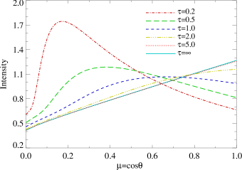
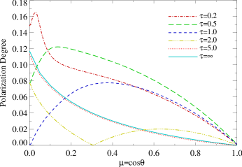
Figure 10.— The polarized spectrum (left) and polarization degree (right) of radiations emerge from the plane-parallel atmosphere of a disk without thickness. The primary photons are isotropically emitted from the central plane of the whole system where the disk located. Radiations can penetrate the disk freely as transporting. Curves with different line styles represent various optical depth of the atmosphere, i.e., $\tau=0.2,0.5,1.0,2.0,5.0,\infty$. Compare to Figure.1 of Dovčiak et al. (2008).

With the procedure presented in the above subsection, we can proceed to calculate the angular distribution of polarization degrees of radiation emerging from the atmosphere of a disk with a finite optical depth $\tau_{1}$ (see the configuration shown in panel (a) of Fig. 1 of Sunyaev & Titarchuk (1985)). The RTE of this system is exactly the same with Eq. (111), except that the primary source is provided explicitly. The source is isotropically and uniformly located on the disk surface (where $\tau=\tau_{1}/2$). The emissivity can be written as $\mathbf{J}(\tau,\mu)=F_{0}\delta(\tau-\tau_{1}/2)(1,0)^{T}$, where $F_{0}$ is a constant. Repeating the same procedure, we can reproduce the results of Fig. 1 of Dovčiak et al. (2008), which were calculated by the public available code STOKES (Goosmann & Gaskell, 2007). Our results are demonstrated in Fig. 10, where $\tau=\tau_{1}/2$. One can compare it with that of Dovčiak et al. (2008) and find that they are in a good agreement. From the figure one can see that as the optical depth increases, the results approach the Chandrasekhar’s Limit eventually.

As we have mentioned in 3.3, one can calculate the results equivalently through another scheme, in which the direction is described by $\Theta,\Phi$. We need trace the polarization vector and construct tetrad, in which the scattering takes place. Thus, this scheme is more complicated and time consuming Compared with the above one.

4.5. Radiations Diffusely Reflected from a Semi-Infinite Plane-Parallel Atmosphere

In this section, we will calculate the angular-dependent polarizations of radiations diffusely reflected from a semi-infinite plane-parallel atmosphere. The incident radiation is a parallel beam with net flux $\mathbf{F}$ per unit area perpendicular to the propagating direction $(-\mu_{0},\varphi_{0})$. Notice that the transport of the fourth component $V$ of the SPs is decoupled from the other three components, we denote $\mathbf{I}=(I,Q,U)^{T}$ and $\mathbf{F}=(F_{I},F_{Q},F_{U})^{T}$. The RTEs governing this system can be written as (Eqs. (101) and (104), Chap. X of Chandrasekhar (1960), page 249)

$$\begin{split}&\displaystyle\mu\frac{d\mathbf{I}(\tau,\mu,\varphi)}{d\tau}=\mathbf{I}(\tau,\mu,\varphi)-\frac{1}{4\pi}\int_{-1}^{+1}\int_{0}^{2\pi}\mathbf{P}(\mu,\varphi;\mu^{\prime},\varphi^{\prime})\times\\ &\mathbf{I}(\tau,\mu^{\prime},\varphi^{\prime})d\mu^{\prime}d\varphi^{\prime}-\frac{1}{4}e^{-\tau/\mu_{0}}\mathbf{P}(\mu,\varphi;-\mu_{0},\varphi_{0})\mathbf{F},\\ &\displaystyle\mu\frac{dV(\tau,\mu,\varphi)}{d\tau}=V(\tau,\mu,\varphi)-\frac{3}{8\pi}\int_{-1}^{+1}\int_{0}^{2\pi}P_{V}(\mu,\varphi;\mu^{\prime},\varphi^{\prime})\times\\ &V(\tau,\mu^{\prime},\varphi^{\prime})d\mu^{\prime}d\varphi^{\prime}-\frac{3}{8}e^{-\tau/\mu_{0}}P_{V}(\mu,\varphi;-\mu_{0},\varphi_{0})F_{V},\\ \end{split}$$ (129)

where $\mathbf{P}$ (given in the Appendix B) is the scattering matrix (or phase-matrix) for $\mathbf{I}$. Since the scattering matrix in terms of $I,Q$ is more suitable for sampling, we prefer to use $I,Q$ rather than $I_{l},I_{r}$, hence the expression of $\mathbf{P}$ adopted here is different with that of Chandrasekhar (1960). The expression of $P_{V}$ reads

$$\displaystyle P_{V}=\mu\mu^{\prime}+\sqrt{1-\mu^{2}}\sqrt{1-\mu^{\prime 2}}\cos(\varphi^{\prime}-\varphi).$$ (130)

From Eq. (129) one can see that the emissivity functions are given by

$$\displaystyle\mathbf{J}=\frac{1}{4}e^{-\tau/\mu_{0}}\mathbf{P}(\mu,\varphi;-\mu_{0},\varphi_{0})\mathbf{F},$$ (131)

$$\displaystyle J_{V}=\frac{3}{8}e^{-\tau/\mu_{0}}P_{V}(\mu,\varphi;-\mu_{0},\varphi_{0})F_{V}.$$ (132)

From which we can get the first sample of the sequence: $P_{1}=(\tau_{1},\mu_{1},\varphi_{1})$ and $\mathbf{\Psi}_{1}$. By sampling $p(\tau)=e^{-\tau/\mu_{0}}$, we can directly obtain $\tau_{1}=-\mu_{0}\ln(1-\xi)$. From the expressions of $\mathbf{J}$ and $J_{V}$, one can see that $(\mu,\varphi)$ is actually the scattered direction for an incident direction $(-\mu_{0},\varphi_{0})$. Thus $(\mu_{1},\varphi_{1})$ can be obtained by sampling a common PDF $f_{I}$ (given by Eq. (C42)) shared by four emissivity functions. Meanwhile the remaining parts are taken as values for $\mathbf{\Psi}_{1}$.

Similarly the next scattering position $\tau_{m+1}$ can be obtained by using Eq. (121) as $\tau_{m}$ is provided. The weight factor $w$ should be multiplied by the factor $A_{1}$ for $\mu_{m}>0$ (and $A_{2}$ for $\mu_{m}<0$), where $A_{1}$ and $A_{s}$ are given by Eq. (118). Since the scattering sampling procedure of generating $(\mu_{m+1},\varphi_{m+1})$ with $(\mu_{m},\varphi_{m})$ provided is very complicated, we will defer the relevant discussions to the Appendix C. After $\mu_{m+1},\varphi_{m+1}$ is obtained, $\mathbf{\Psi}_{m+1}$ should be updated according to Eq. (C59). Analogously, once a sequence of $P_{i}$ and $\mathbf{\Psi}_{i}$ ($i=1,2,\cdots$) is generated, the estimations for $\mathbf{I}_{m}$ and $V_{m}$ can be obtained as

$$\begin{split}\left\{\begin{array}[]{ll}&\displaystyle F^{(X)}_{m}=w\cdot f_{X}(\mathbf{\Omega}_{\text{obs}};\mathbf{\Omega}_{m-1})\cdot\Psi^{(I)}_{m-1}\cdot f_{m},\\ &F^{(V)}_{m}=w\cdot f_{V}(\mathbf{\Omega}_{\text{obs}};\mathbf{\Omega}_{m-1})\cdot\Psi^{(V)}_{m-1}\cdot f_{m},\end{array}\right.\end{split}$$ (133)

where $X$ can be $I,Q,U$, and

$$\begin{split}&f_{m}=\displaystyle\frac{1}{\mu_{\text{obs}}}\exp\left(-\frac{\tau_{m}}{\mu_{\text{obs}}}\right),\end{split}$$ (134)

is the recording function. Repeating this procedure, the angular-dependent diffusely reflected spectrum can be eventually generated.

We first reproduce the results of Fig. 11 of Schnittman & Krolik (2013), which mainly illustrate the distributions of radiations diffusely reflected forward and backward in the incident plane (where $\varphi-\varphi_{0}=0^{\circ},180^{\circ}$) and the plane perpendicular to it (where $\varphi-\varphi_{0}=90^{\circ},270^{\circ}$), respectively. Due to the symmetry, the radiations reflected to the directions at $\varphi-\varphi_{0}=90^{\circ}$ and $270^{\circ}$ are exactly the same, we can put them together in the plotting. The angles of incident beam are $\varphi_{0}=0$ and $\mu_{0}=0.2,0.5,0.8$ for three cases and the beam is polarized with the SPs given by $F_{Q}=F_{I}/4$, $F_{U}=F_{I}/4$ and $F_{V}=F_{I}/4$. The results are shown in Fig. 11, 12 and 13, in which the semi-analytical results of Chandrasekhar (1960) for diffuse reflection are also plotted. They can be obtained directly from the well know formula of Chandrasekhar (1960) given by

$$\displaystyle\mathbf{I}(\tau=0,\mu,\varphi)=\left(\begin{array}[]{c}I_{l}\\ I_{r}\\ U\\ V\end{array}\right)=\frac{1}{4\mu}\mathbf{Q}\mathbf{S}(\mu,\varphi;-\mu_{0},\varphi_{0})\left(\begin{array}[]{c}F_{l}\\ F_{r}\\ F_{U}\\ F_{V}\end{array}\right),\quad\quad$$ (143)

where $F_{l},F_{r},F_{U}$ are the SPs of the incident radiation. From these figures, one can see that the two results coincide with each other very well. Comparing to the cases with unpolarized incident beams, the polarized incident radiation will give rise to a nonzero reflected $U$.

Figure 11.— SPs of radiations diffusely reflected from a semi-infinite plane-parallel atmosphere distribute with respect to the polar angle in the incident plane ($\varphi-\varphi_{0}=0^{\circ},180^{\circ}$, left panel) and the plane perpendicular to it ($\varphi-\varphi_{0}=90^{\circ},270^{\circ}$, right panel). The direction of the incident parallel beam is $\mu_{0}=0.2,\varphi_{0}=0$. And the incident beam is polarized with SPs given by $F_{Q}=F_{I}/4$, $F_{U}=F_{I}/4$ and $F_{V}=F_{I}/4$. The solid and dotted lines represent the results calculated by the semi-analytical formula of Chandrasekhar (1960) and our MC scheme, respectively. Compare to Figure 24 of Chandrasekhar (1960).

Figure 12.— Same as in Figure 11, but for $\mu_{0}=0.5$. Compare to Figure 25 of Chandrasekhar (1960).

Figure 13.— Same as in Figure 11, but for $\mu_{0}=0.8$. Compare to Figure 26 of Chandrasekhar (1960).

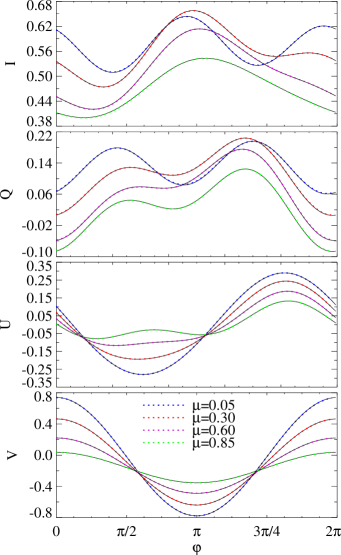
Figure 14.— The distribution of I, Q, U, V of radiations diffusely reflected from a plane-parallel atmosphere with respect to the azimuth angle $\varphi$ for various cosines of viewing angles, i.e., $\mu=0.05,0.3,0.6,0.85$, respectively. The incident radiation is polarized and has a direction of $\mu_{0}=0.5$ and $\varphi_{0}=0$. The solid and dotted lines represent the results calculated by the semi-analytical formula of Eq. (143) and our MC scheme, respectively.

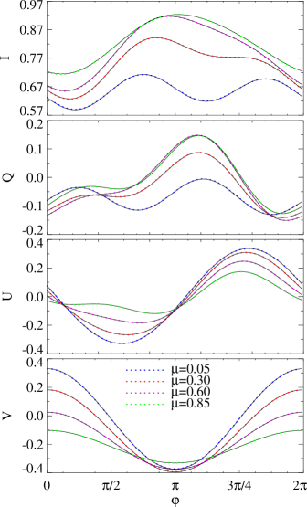
Figure 15.— Same as in Figure 14, but for $\mu_{0}=0.8$.

We proceed to demonstrate the SPs of diffusely reflected radiations distributed with respect to the azimuth angle $\varphi$ for various observational angles in Fig. 14 and 15. The incident radiation is also polarized with the same manner given above. For comparison, we also plot the semi-analytical results of Chandrasekhar (1960). In our calculations, the maximum optical depth along the vertical direction of the atmosphere is set to be $\tau=100$. From these Figures one can see that as $\mu$ decrease (the escaped radiations will travel through a higher optical depth and be scattered sufficiently by the atmosphere), the maxima and minima of the SPs show a period of $\pi$ and $2\pi$ approximately, because the functions of $\cos 2\varphi$ and $\sin 2\varphi$ appear in the scattering matrix. One can find that these results agree with each other very well.

4.6. the Transmission through a Plane-Parallel Atmosphere

With the preparations given in the last subsection, we can readily reproduce the SPs distributions of radiations transmitted through a plane-parallel atmosphere with a finite optical depth $\tau_{0}$. The transmission process obeys exactly the same RTEs given by Eqs. (129) and the unpolarized parallel incident radiations are injected from the bottom boundary ($\tau=\tau_{0}$). The cosines of incident polar angles are $\mu_{0}=0.1,0.2,0.4,0.5,0.8$ respectively and azimuth angle $\varphi_{0}=0^{\circ}$. In order to compare with the results of Fig. 27 of Chandrasekhar (1960), here we only consider the transmitted radiations lying in the incident plane, i.e., $\varphi-\varphi_{0}=0^{\circ},180^{\circ}$ and $\theta\in[0^{\circ},90^{\circ}]$. The result is shown in Fig. 16, where the SPs $U$ and $V$ are also provided. For the sake of clarity, each curve has been displaced by a distance along the y-axis. In the second panel, the black spots indicate the neutral points of $Q$, which correspond to Babinet (Ba), Brewster (Br) and Arago (A) points respectively. One can see that the U component vanishes, which is due to the left and right symmetry of the observer that is located in the incident plane of the beam. Comparing with Fig. 27 of Chandrasekhar (1960), one can find that the results are consistent.

Figure 16.— The SPs of radiations transmitted through a plane-parallel atmosphere distribute with respect to the polar angle $\theta$. Curves from top to bottom in each panel correspond to different cosines of incident polar angles, $\cos\theta_{0}=0.1,0.2,0.4,0.5,0.8$, respectively. In the second panel, the spots indicate the neutral points where $Q$ changes its signs. Compare to Fig. 27 of Chandrasekhar (1960).

4.7. Anisotropic Comptonization in Thermal Plasma

The inverse Compton scattering is one of most important mechanisms that can produce high-energy photons, such as X-rays and $\gamma$-rays, by scattering low-frequency radiations against hot or relativistic electron gas (Younsi & Wu, 2013). This mechanism has been extensively studied by analytical method (Haardt, 1993), numerical method (Poutanen & Svensson, 1996a) and MC method (Pozdnyakov et al., 1983; Hua & Titarchuk, 1995; Hua, 1997; Dolence et al., 2009). In our MC scheme based on Neumann solution, we have shown that the MCRT amounts to calculate infinite multiple integrals simultaneously, and the Compton scattering can be completely regarded as a sampling procedure of a PDF with an integral form given by Eq. (28). The sampling and estimation procedures for them have been thoroughly discussed in the section. 2.4.2 and the polarized case are given in the section. 3.1. For scattering sampling, we always make a Lorentz transformation and get into the rest frame of the electron, in which the formula of scattering will be simplified. For estimations, after eliminating the $\delta$-function in the recording function, we take $C(\nu,\mathbf{\Omega}\rightarrow\nu^{\prime},\mathbf{\Omega}_{\text{obs}})$ as a weight. Usually when $\nu,\mathbf{\Omega},\mathbf{\Omega}^{\prime}$ are specified, the scattered frequency $\nu^{\prime}$ is uniquely determined, $C$ is also completely determined. If the scattering of $\nu$ and $\mathbf{\Omega}$ are independent, we can determine $C$ by introducing another $\delta$ function $\delta(\nu^{\prime}-\nu_{\text{obs}})$ to replace $\nu^{\prime}$ by $\nu_{\text{obs}}$. For averaged Compton scattering, the kernel is given by Eq. (32). To determine $C$, we need finish the integrals in terms of $\gamma,\mu_{e}$ and $\phi_{e}$. As aforementioned, this can be done by the MC method, i.e., we sample $f_{e}(P_{e})$ directly and take the rest of the integrand as the weight, which is given by

$$\begin{split}&\displaystyle w_{s}=\frac{1}{\sigma_{\text{KN}}(\epsilon)}\frac{d\sigma_{\text{KN}}}{d\mu_{e}^{\prime}\phi_{e}^{\prime}},\end{split}$$ (144)

Then the recording function becomes

$$\begin{split}\begin{array}[]{l}\displaystyle f_{\text{new}}=\displaystyle w_{s}\exp\left[-\tau(\mathbf{r},\nu^{\prime},\mathbf{\Omega}_{\text{obs}})\right].\end{array}\end{split}$$ (145)

To verify the correctness of this scheme, we first apply it to calculate the Comptonized spectrum of low-energy radiation by the thermal plasma in a plane-parallel atmosphere. This Comptonization process has been calculated by Haardt (1993). They treated this transfer process by using a semi-analytical formalism and compared it with the results obtained from the MC method. This computation is quite suitable to check our scheme. The low-energy thermal photons are injected from the bottom surface of the atmosphere. The incident intensity is angular-dependent and simply given by (Haardt, 1993)

$$\begin{split}&\displaystyle U_{0}(\mu)=\left\{\begin{array}[]{lrl}\displaystyle\frac{6}{3+2b}(\mu+b\mu^{2}),&0&<\mu<1;\\ \displaystyle 0,&-1&<\mu<0,\\ \end{array}\right.\\ \end{split}$$ (146)

where $b$ is a constant and set to be $2$ in the practical calculation. Obviously $U_{0}(\mu)$ gives rise to a limb-darkening law for the incident radiations.

Our results is shown in Figs. 17-20, corresponding to Figs. 2-6 of Haardt (1993). Figs. 17-19 demonstrate the total Comptonized spectra together with the spectra of each single scattering. The spectra vary with different optical depth, plasma temperature and observational angle. Fig. 20 shows how the total spectrum changes with the viewing angles, especially for $\mu<0$, corresponding to the spectrum reflected back from the atmosphere. One can see that our results are consistent with that of Haardt (1993).

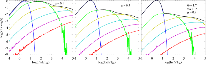
Figure 17.— The Comptonized spectra of low-energy thermal radiations by a hot plasma atmosphere. The total spectrum (solid black line) and each single scattering contributions are shown together. The dimensionless temperature and optical depth for the hot plasma are $\Theta=1.7$ and $\tau=0.15$. The cosines of the viewing angles are $\mu=0.1$, $0.5$ and $0.9$ for panels from left to right, respectively. The observed photon energies are in unit of $kT_{\text{bb}}$, which is the temperature of the incident thermal radiation. Compare to Fig. 2 of Haardt (1993).

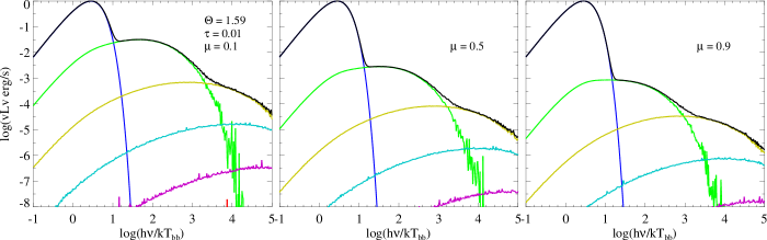
Figure 18.— Same as in Figure 17, but for $\Theta=1.59$ and $\tau=0.01$. Compare to Fig. 3 of Haardt (1993).

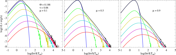
Figure 19.— Same as in Figure 17, but for $\Theta=0.188$ and $\tau=0.06$. Compare to Fig. 4 of Haardt (1993).

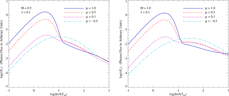
Figure 20.— The inverse Comptonized spectra of low-energy thermal radiations by a hot plasma atmosphere for various viewing angles. The parameters for the hot plasma are $\Theta=0.5$, $\tau=0.1$ and $\Theta=1.0$, $\tau=0.1$ for left and right panels, respectively. Compare to Figs. 5 and 6 of Haardt (1993).

4.8. The First Order Green’s Function For Relativistic Compton Reflection

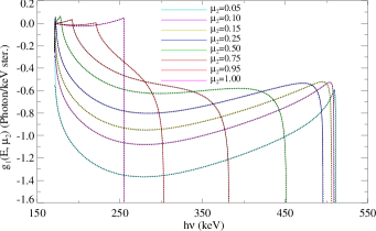
Figure 21.— The first-order Green’s function for monoenergetic incident photons with 511 keV reflected from a semi-infinite atmosphere of cold electron. The curves with different colors correspond to different values of the cosines of viewing angle $\mu_{2}$. The solid and dotted lines represent the results calculated by the analytical formulae of Hua & Lingenfelter (1992) and our MC scheme, respectively. Compare to Fig. 1 in Hua & Lingenfelter (1992).

With the above discussed strategy, we will reproduce the calculations of Hua & Lingenfelter (1992) for the first order Green’s functions of relativistic Compton reflection by a semi-infinite plane-parallel atmosphere of cold electrons. Hua & Lingenfelter (1992) have shown that the first order Green’s function for such a system has an analytical expression and is strongly dependent on the viewing angles of the atmosphere. Since the cold electrons can be approximately regarded as static, we do not have to consider any electron sampling process and Lorentz transformation at all. The unpolarized and monoenergetic (511 keV) photons are isotropically injected from all directions to the surface of the atmosphere. The Green’s function can be expressed as an expansion of functions characterized by the number of scattering times (Hua & Lingenfelter, 1992)

$$\displaystyle G(E,\mu_{2})=\sum_{n=1}^{\infty}g_{n}(E,\mu_{2}),$$ (147)

where $E$ is the escaping energy of the photon, $\mu_{2}$ is the cosine of the viewing polar angle $\theta_{2}$. Using the the MC method, one can easily obtain the numerical result for any function $g_{n}$ in this series. In our scheme, we simply have

$$\begin{split}&g_{n}(E,\mu_{2})=\displaystyle\int\cdots\int S(P_{0})K(P_{0}\rightarrow P_{1})\cdots\\ &\times K(P_{n-1}\rightarrow P_{n})f(P_{n})\delta(\mu-\mu_{2})dP_{0}dP_{1}\cdots dP_{n}.\end{split}$$ (148)

Here we mainly care about the first order $g_{1}(E,\mu_{2})$, i.e.,

$$\begin{split}&g_{1}(E,\mu_{2})=\displaystyle\iint S(P_{0})K(P_{0}\rightarrow P_{1})\\ &\times f(P_{1})\delta(\mu-\mu_{2})dP_{0}dP_{1},\end{split}$$ (149)

which has been analytically integrated by Hua & Lingenfelter (1992).

For a given viewing angle, there is a cut-off energy (Hua & Lingenfelter, 1992)

$$\displaystyle E_{\text{cutoff}}=\frac{511}{2-\sqrt{1-\mu_{2}^{2}}}\text{ keV},$$ (150)

above which no reflected photon can be seen. The results of $g_{1}$ for various $\mu_{2}$ are plotted in Fig. (21), where the analytical results of Hua & Lingenfelter (1992) are also shown for comparison. One can see that the agreement between these results is quite well.

4.9. Comptonization of Polarized Radiation from a Reflecting Disk with a Hot Corona

In the last two applications, we mainly focus on the unpolarized Compton scattering dominated RT. In this section we proceed to discuss the applications with polarization and calculate the analogous spectra emerging from the hot corona of an optically thick disk. The effect that radiations can be reflected from the disk when they irradiate the disk surface is also considered. The reflected radiation $\mathbf{I}_{r}$ in the direction of $\mathbf{\Omega}$ equals the sum of contributions coming from all other incident directions $\mathbf{\Omega}^{\prime}$, i.e., (Poutanen et al., 1996b),

$$\begin{split}\mathbf{I}_{r}(\nu,\mathbf{\Omega})&=\int\mathbf{G}(\nu,\mathbf{\Omega};\nu^{\prime},\mathbf{\Omega}^{\prime})\mathbf{I}(\nu^{\prime},\mathbf{\Omega}^{\prime})d\nu^{\prime}d\mathbf{\Omega}^{\prime}.\end{split}$$ (151)

where $\mathbf{G}(\mathbf{\Omega},\nu;\mathbf{\Omega}^{\prime},\nu^{\prime})$ is the Green function obtained by solving the RT process in the disk (Magdziarz & Zdziarski, 1995). The matrix function $\mathbf{QS}/4\mu$ in Eq. (143) is actually such a Green function. We will use it to get the reflected radiations. In Appendix E, we discussed how to incorporate the reflection term $\mathbf{I}_{r}$ into the integral equation and sample the modified transfer kernel.

As aforementioned the transformation between the incident and Compton scattered Stokes parameters are given by Eqs. (69) and (70). Considering the distribution of electron gas and the unpolarized situation, this transformation formula should be modified as

$$\begin{split}&\displaystyle\mathbf{\Psi}^{\prime}=\frac{1}{4\pi}\int_{1}^{\infty}d\gamma N_{e}(\gamma)\int_{-1}^{1}d\mu_{e}(1-\mu_{e}v)\int_{0}^{2\pi}d\varphi_{e}\\ &\times\frac{r^{2}_{e}}{\gamma^{2}(1-\mu_{e}v)^{2}}\left(\frac{\nu^{\prime}}{\nu}\right)^{2}\mathbf{FM}(\varphi)\mathbf{\Psi}.\end{split}$$ (152)

Similarly the integrals in the above equation can be evaluated by sampling a set of $\gamma,\mu_{e},\varphi_{e}$. With them and after the multiplication of matrices $\mathbf{FM}(\varphi)$ and $\mathbf{\Psi}$, we have

$$\begin{split}&\displaystyle\Psi^{\prime(X)}=A_{0}f_{X}(\mu^{\prime},\varphi^{\prime};\mu,\varphi)\Psi^{(I)},\\ &\displaystyle\Psi^{\prime(V)}=A_{0}f_{V}(\mu^{\prime},\varphi^{\prime};\mu,\varphi)\Psi^{(V)},\end{split}$$ (153)

where $A_{0}=(r^{2}_{e}/2)(\epsilon^{\prime}/\epsilon)^{2}/\sigma_{\text{KN}}(\epsilon)$ and $X=(I,Q,U)$. Transforming $f_{X}$ and $f_{V}$ into the rest frame of the electron, we have

$$\left\{\begin{array}[]{ll}&\displaystyle\widetilde{f_{I}}=F_{0}+F_{3}(q\cos 2\Phi^{\prime}+u\sin 2\Phi^{\prime}),\\ &\displaystyle\widetilde{f_{Q}}=F_{3}+F_{33}(q\cos 2\Phi^{\prime}+u\sin 2\Phi^{\prime}),\\ &\displaystyle\widetilde{f_{U}}=F_{11}(-q\sin 2\Phi^{\prime}+u\cos 2\Phi^{\prime}),\\ &\displaystyle\widetilde{f_{V}}=F_{22},\end{array}\right.$$ (158)

where $q=\Psi^{(Q)}/\Psi^{(I)},u=\Psi^{(U)}/\Psi^{(I)}$, and $(\Psi^{\prime},\Phi^{\prime})$ are the scattered polar and azimuth angles in the rest frame of the electron. We also use $A_{0}\widetilde{f_{I}}$ to construct a PDF for $(\Psi^{\prime},\Phi^{\prime})$ and sample it to get the scattered direction. After transforming it back into the static frame, we get $(\mu^{\prime},\varphi^{\prime})$ and the scattered $\mathbf{\Psi}^{\prime}$ as

$$\left\{\begin{array}[]{ll}&\displaystyle\Psi^{\prime(X)}=\frac{f_{X}(\mu^{\prime},\varphi^{\prime};\mu,\varphi)}{f_{I}(\mu^{\prime},\varphi^{\prime};\mu,\varphi)}\Psi^{(I)},\\ &\displaystyle\Psi^{\prime(V)}=\frac{f_{V}(\mu^{\prime},\varphi^{\prime};\mu,\varphi)}{f_{I}(\mu^{\prime},\varphi^{\prime};\mu,\varphi)}\Psi^{(V)}.\end{array}\right.$$ (161)

The estimation functions for the Stokes parameters are given by

$$\left\{\begin{array}[]{ll}&\displaystyle F_{X}=A_{0}\widetilde{f_{X}}(\mathbf{\Omega}_{\text{obs}})\Psi^{(I)}_{m}\exp\left[-\tau(\nu,\mathbf{\Omega}_{\text{obs}})\right],\\ &\displaystyle F_{V}=A_{0}\widetilde{f_{V}}(\mathbf{\Omega}_{\text{obs}})\Psi^{(V)}_{m}\exp\left[-\tau(\nu,\mathbf{\Omega}_{\text{obs}})\right].\end{array}\right.$$ (164)

With these preparations, we can now proceed to complete the calculations mentioned at the beginning of this section. The source thermal radiation has a temperature $kT_{bb}=10$ eV and is located isotropically and uniformly on the disk surface. The radiations scattered back into the disk will re-emerge with an altered SPs determined by Eq. (143). The results are plotted in Figs. 22 and 23. The corona temperature and Thomson optical depth are $T_{e}$ and $\tau=h\sigma_{T}n_{e}$, where $h$ is the height of corona. The values of these parameters correspond to those of Figs. 5 and 6 of Poutanen & Svensson (1996a) (also refer to Figs 12 and 13 of Schnittman & Krolik (2013)). One can see that our results are similar but different with them, especially for the curves corresponding to each single scattering. In our scheme, since each scattering (including the reflection) can make contributions to the spectra, we do not reset the variable of scattering number $N_{\text{scat}}$ to zero after the photons are reflected from the disk. It is contrast to the treatment of Schnittman & Krolik (2013). The reflection processes are described by Eq. (143), where the photoelectric absorption and energy losses due to Compton recoil are not considered. Therefore the reflection processes will not change the energies of photons. We believe that these different treatments give rise to the discrepancies in the spectra profiles and the polarization degrees.

One can see that the high energy parts of the spectra, almost greater than $\sim 100$ keV, are quite noise and oscillate heavily, because the photons received by the observer at that energy band have experienced a large averaged scattering number. The weights of these photons have been attenuated heavily, hence the polarization signals comprised by these weights are difficult to be resolved (Schnittman & Krolik, 2013).

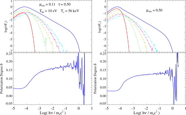
Figure 22.— The spectra (top panels) and polarization degrees (bottom panels) of radiations emerging from a plane-parallel corona above an accretion disk. The solid blue curves correspond to the total spectra and the solid red, dotted, dashed, dot-dashed, triple-dot-dashed curves correspond to scattering number of 0, 1, 2, 3, 4, respectively. Compare to Figure 5 of Poutanen & Svensson (1996a).

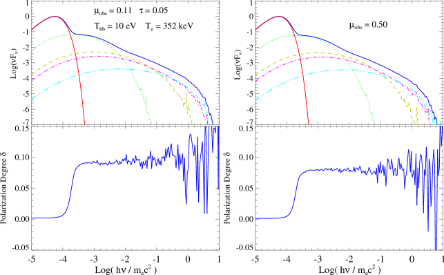
Figure 23.— The same as in Fig. 22, but for $T_{e}=353$ keV and $\tau=0.05$. Compare to Figure 6 of Poutanen & Svensson (1996a).

4.10. The Scattering of Polarized Photon Beam by Relativistic Electrons

In this section we will consider the polarization states of a polarized photon beam scattered off only once by a relativistic electron gas that can have an arbitrary distribution function $N_{e}(\gamma)$. We denote the energies, polarization and wave vectors for the incident and scattered photons as $\epsilon,\boldsymbol{\varepsilon},\mathbf{k}$ and $\epsilon^{\prime},\boldsymbol{\varepsilon}^{\prime},\mathbf{k}^{\prime}$ respectively, and the scattering angle between $\mathbf{k}$ and $\mathbf{k}^{\prime}$ is $\theta^{\prime}$. Then the scattered intensity can be expressed semi-analytically as follows (Bonometto et al., 1970; Bonometto & Saggion, 1973a, b)

$$\begin{split}J_{\boldsymbol{\varepsilon}^{\prime}}&=\pi\left(\frac{e^{2}}{4\pi}\right)\frac{\epsilon^{\prime}}{\epsilon}E_{\text{min}}\left\{\left|\boldsymbol{\varepsilon}\cdot\boldsymbol{\varepsilon}^{\prime*}+\frac{(\mathbf{k}\cdot\boldsymbol{\varepsilon}^{\prime*})(\mathbf{k}^{\prime}\cdot\boldsymbol{\varepsilon})}{1-\cos\theta^{\prime}}\right|^{2}\Sigma_{1}\right.\\ &\left.+\left|\boldsymbol{\varepsilon}\cdot\boldsymbol{\varepsilon}^{\prime}+\frac{(\mathbf{k}\cdot\boldsymbol{\varepsilon}^{\prime})(\mathbf{k}^{\prime}\cdot\boldsymbol{\varepsilon})}{1-\cos\theta^{\prime}}\right|^{2}\Sigma_{2}+\Sigma_{2}\right\},\end{split}$$ (165)

where

$$\begin{split}&\displaystyle\Sigma_{1}=\int_{0}^{1}m(\gamma)\left(x^{2}-\frac{1}{x^{2}}+2\right)dx,\\ &\displaystyle\Sigma_{2}=\int_{0}^{1}m(\gamma)\frac{(1-x^{2})^{2}}{x^{2}}dx,\\ &\displaystyle x=\frac{E_{\text{min}}}{\gamma},\quad\quad E_{\text{min}}=\sqrt{\frac{1}{2}\frac{\epsilon^{\prime}}{\epsilon}\frac{1}{(1-\cos\theta^{\prime})}},\end{split}$$ (166)

and the quantity $m(\gamma)$ is related to $N_{e}(\gamma)$, and

$$\begin{split}m(\gamma)=\frac{N_{e}(\gamma)}{\gamma^{2}}.\end{split}$$ (167)

For simplicity we denote $\displaystyle J_{0}=\pi\left(\frac{e^{2}}{4\pi}\right)\frac{\epsilon^{\prime}}{\epsilon}E_{\text{min}}$. Using the base vectors $\Ket{\mathbf{e}_{x}},\Ket{\mathbf{e}_{y}}$, the polarization vectors $\boldsymbol{\varepsilon}$ and $\boldsymbol{\varepsilon}^{\prime}$ can be decomposed as

$$\begin{split}\boldsymbol{\varepsilon}=\alpha\Ket{\mathbf{e}_{x}}+\beta\Ket{\mathbf{e}_{y}},\quad\boldsymbol{\varepsilon}^{\prime}=\alpha^{\prime}\Ket{\mathbf{e}^{\prime}_{x}}+\beta^{\prime}\Ket{\mathbf{e}^{\prime}_{y}}.\end{split}$$ (168)

Then with $\alpha,\beta$ and $\alpha^{\prime},\beta^{\prime}$, Eq. (165) can be recast as (Bonometto et al., 1970)

$$\begin{split}J_{\boldsymbol{\varepsilon}^{\prime}}&=J_{0}\left\{c_{1}\Sigma_{1}+c_{2}\Sigma_{2}+\Sigma_{2}\right\}.\end{split}$$ (169)

where $c_{1}=\left|\alpha\alpha^{\prime*}-\beta\beta^{\prime*}\right|^{2}$ and $c_{2}=\left|\alpha\alpha^{\prime}-\beta\beta^{\prime}\right|^{2}$. Without loss of generality, one can choose $\alpha=x,\,\beta=ye^{i\theta}$ (obviously $x^{2}+y^{2}=1$), the coefficients $c_{1}$ and $c_{2}$ can be written as

$$\begin{split}c_{1}&=x^{2}x^{\prime 2}-2xx^{\prime}yy^{\prime}\cos(\theta-\theta^{\prime})+y^{2}y^{\prime 2},\\ c_{2}&=x^{2}x^{\prime 2}-2xx^{\prime}yy^{\prime}\cos(\theta+\theta^{\prime})+y^{2}y^{\prime 2}.\end{split}$$ (170)

Usually we describe the polarization state by SPs: $I,Q,U,V$ or the normalized SPs: $\xi_{1}=U/I,\,\xi_{2}=V/I,\,\xi_{3}=Q/I$. For simplicity we define a vector $\mathbf{S}=(1,\xi_{3},\xi_{1},\xi_{2})$. By using Eq. (56), we can immediately obtain $\xi_{i}$ from $x,y$ and $\theta$:

$$\begin{split}&\xi_{1}=2xy\cos\theta,\quad\xi_{2}=2xy\sin\theta,\quad\xi_{3}=x^{2}-y^{2},\end{split}$$ (171)

and vice versa

$$\begin{split}&x=\sqrt{\frac{1+\xi_{3}}{2}},\quad y=\sqrt{\frac{1-\xi_{3}}{2}},\\ &\cos\theta=\frac{\xi_{1}}{\sqrt{\xi_{1}^{2}+\xi_{2}^{2}}},\quad\sin\theta=\frac{\xi_{2}}{\sqrt{\xi_{1}^{2}+\xi_{2}^{2}}}.\end{split}$$ (172)

For any two orthogonal polarization states of $\boldsymbol{\varepsilon}=(\alpha,\beta)$ and $\boldsymbol{\varepsilon}_{\perp}=(\alpha_{\perp},\beta_{\perp})$, since $\boldsymbol{\varepsilon}\cdot\boldsymbol{\varepsilon}_{\perp}^{*}=\alpha\alpha_{\perp}^{*}+\beta\beta_{\perp}^{*}=0$, without loss of generality we can obtain $\boldsymbol{\varepsilon}_{\perp}=(-\beta^{*},\alpha^{*})$. Using Eq. (56), one can immediately obtain that the normalized SPs for $\boldsymbol{\varepsilon}_{\perp}$ is $\mathbf{S}_{\boldsymbol{\varepsilon}_{\perp}}=(1,-\xi_{3},-\xi_{1},-\xi_{2})$ if the corresponding ones for $\boldsymbol{\varepsilon}$ is $\mathbf{S}_{\boldsymbol{\varepsilon}}=(1,\xi_{3},\xi_{1},\xi_{2})$. The total intensity for the scattered radiation is the sum of $J_{\boldsymbol{\varepsilon}^{\prime}}$ over any two orthonormal polarization states, and one can easily obtain (Bonometto et al., 1970)

$$\begin{split}J_{I^{\prime}}=J_{\boldsymbol{\varepsilon}^{\prime}}+J_{\boldsymbol{\varepsilon}^{\prime}_{\perp}}=J_{0}\left\{\Sigma_{1}+3\Sigma_{2}\right\}.\end{split}$$ (173)

Due to the additive property of SPs (Chandrasekhar, 1960), the normalized SPs for $J_{I^{\prime}}$ is $\mathbf{S}_{I^{\prime}}=\mathbf{S}_{\boldsymbol{\varepsilon}^{\prime}}+\mathbf{S}_{\boldsymbol{\varepsilon}^{\prime}_{\perp}}=(1,0,0,0)$.

Similarly, the scattered intensity for the polarization state of $Q^{\prime}$ is given by

$$\begin{split}J_{Q^{\prime}}&=J_{S^{\prime}_{+}}-J_{S^{\prime}_{-}}\\ &=J_{0}\left[(c_{1}^{+}-c_{1}^{-})\Sigma_{1}+(c_{2}^{+}-c_{2}^{-})\Sigma_{2}\right],\end{split}$$ (174)

where $\mathbf{S}^{\prime}_{\pm}=(1,\pm 1,0,0)$. The corresponding coefficients $c_{1}^{\pm}$ and $c_{2}^{\pm}$ are obtained from Eq. (170). Similarly, the scattered intensities for polarization states $U^{\prime}$ and $V^{\prime}$ are given by

$$\begin{split}J_{U^{\prime}}&=J_{S^{\prime}_{+}}-J_{S^{\prime}_{-}}\\ &=J_{0}\left[(c_{1}^{+}-c_{1}^{-})\Sigma_{1}+(c_{2}^{+}-c_{2}^{-})\Sigma_{2}\right],\\ J_{V^{\prime}}&=J_{S^{\prime}_{+}}-J_{S^{\prime}_{-}}\\ &=J_{0}\left[(c_{1}^{+}-c_{1}^{-})\Sigma_{1}+(c_{2}^{+}-c_{2}^{-})\Sigma_{2}\right],\end{split}$$ (175)

where the coefficients $c_{1}^{\pm}$ and $c_{2}^{\pm}$ are obtained from the normalized SPs $\mathbf{S}^{\prime}_{\pm}=(1,0,\pm 1,0)$ for $U^{\prime}$ and $\mathbf{S}^{\prime}_{\pm}=(1,0,0,\pm 1)$ for $V^{\prime}$, respectively. Since any polarization state is completely determined by SPs, therefore once $J_{I^{\prime}},J_{Q^{\prime}},J_{U^{\prime}},J_{V^{\prime}}$ are obtained, the scattered polarization state is also determined.

With these preparations, we can readily obtain the scattered polarization states semi-analytically, which can be used to verify our MC scheme. We first reproduce the results in Fig. 2 of Mościbrodzka (2020), where four polarized incident beams are scattered off by a group of hot electron gas distributed according to the relativistic Maxwell function (see Eq. (27)). The dimensionless temperature of the gas is $\Theta_{e}=kT_{e}/m_{e}c^{2}=100$. The incident beams with fixed energy $\epsilon=2.5\times 10^{-11}$ propagate along the positive $z$-axis and the viewing direction is $(\theta^{\prime},\varphi^{\prime})=(85^{\circ},0)$. The normalized SPs of the four incident beams are $\mathbf{S}_{\text{in},1}=(1,1,0,0)$, $\mathbf{S}_{\text{in},2}=(1,-1,0,0)$, $\mathbf{S}_{\text{in},3}=(1,0,1,0)$, and $\mathbf{S}_{\text{in},4}=(1,0,0,1)$, respectively. The scattered intensities for all beams are the same and independent on the polarizations of the incident beams (see Eq. (173)). The intensity (left panel) and fractional polarizations (right panel) of the scattered photons distributed with respect to the photon energy are shown in Fig. 24, where only the nonvanishing normalized SPs are plotted. One can see that the numerical results produced by our MC scheme agree with the semi-analytical results of Bonometto et al. (1970) very well, especially in the low energy band. The noise of the high energy part is relatively large due to the sparse productions of energetic photons comparing to that of the low energy ones.

Next we consider the case where the electron gas is distributed in a power law profile, i.e.,

$$N_{e}(\gamma)=K\gamma^{-\alpha},\quad\gamma\geq\gamma_{1},$$ (176)

where $K=(\alpha-1)/\gamma_{1}^{1-\alpha}$ is the normalization factor and $\alpha$ is the power law index. Then $m(\gamma)=K\gamma^{-(\alpha+2)}$, one can immediately obtain the expressions for quantities $\Sigma_{1}$ and $\Sigma_{2}$ as (Bonometto et al. (1970))

$$\begin{split}\Sigma_{1}=\frac{K}{E^{\alpha+1}_{\text{min}}}x_{1}^{\alpha+1}\left[\frac{x_{1}^{4}}{\alpha+5}-\frac{1}{\alpha+1}+\frac{2x_{1}^{2}}{\alpha+3}\right],\\ \Sigma_{2}=\frac{K}{E^{\alpha+1}_{\text{min}}}x_{1}^{\alpha+1}\left[\frac{x_{1}^{4}}{\alpha+5}+\frac{1}{\alpha+1}-\frac{2x_{1}^{2}}{\alpha+3}\right],\end{split}$$ (177)

where (notice that $E_{\text{min}}$ is dependent on the energies of scattered photons)

$$x_{1}=\left\{\begin{array}[]{lr}\displaystyle 1,&\quad\quad\text{ if }E_{\text{min}}\geq\gamma_{1},\\ \displaystyle\frac{E_{\text{min}}}{\gamma_{1}},&\quad\quad\text{ if }E_{\text{min}}<\gamma_{1}.\end{array}\right.$$ (180)

Our results in comparison with the analytic ones of Bonometto et al. (1970) are shown in Figs. 25 and 26. In these calculations we set $\gamma_{1}=60.0$, the power law index $\alpha=3$ and the incident monoenergy $\epsilon=2.5\times 10^{-11}$. Using the inverse CDF method, we can easily sample $\gamma$ from $N_{e}(\gamma)$, i.e., $\gamma_{\xi}=\gamma_{1}(1-\xi)^{1/(1-\alpha)}$. From Eq. (177) one can see that there exist a turning point $\epsilon^{\prime}_{\text{tr}}$ for the scattered photon energy $\epsilon^{\prime}$, above which all of the fractional polarizations: $\xi_{3},\xi_{2},\xi_{1}$ are constants (but notice that the SPs $I,Q,U,V$ are not). From the condition $E_{\text{min}}=\gamma_{1}$ one can easily obtain that $\epsilon^{\prime}_{\text{tr}}/\epsilon=2(1-\cos\theta^{\prime})\gamma_{1}^{2}$. In Figs. 25 and 26, where $\theta^{\prime}=85^{\circ}$ and $\gamma_{1}=60.0$, we have $\log_{10}(\epsilon^{\prime}_{\text{tr}}/\epsilon)\approx 3.818$. The normalized SPs of the four incident beams in Fig. 25 are the same with those in Fig. 24. While in Fig. 26, the incident SPs are $\mathbf{S}_{\text{in}}=(1,0.25,0.433,0.866)$ and all of the scattered SPs are nonvanishing.

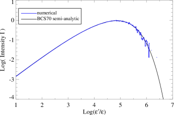
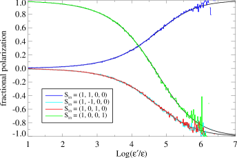
Figure 24.— The intensity (left) and normalized SPs (right) of photons scattered off a group of thermal relativistic electron gas with various incident polarizations $\mathbf{S}_{\text{in}}$. The dimensionless temperature of the electron gas is $\Theta_{e}=100$. The incident energy is monoenergetic and $\epsilon=h\omega/m_{e}c^{2}=2.5\times 10^{-11}$. The solid lines and histograms represent the results obtained by the semi-analytical formulae of Bonometto et al. (1970) and our MC scheme, respectively. Compare to Fig. 2 of Mościbrodzka (2020).

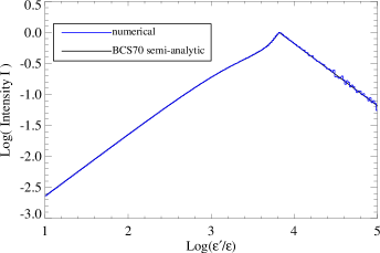
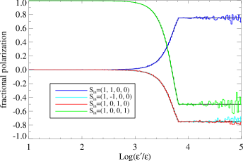
Figure 25.— Same as in Fig. 24, but the electron gas is distributed in a power law profile given be Eq. (176), where $\gamma_{1}=60.0$, $\alpha=3$ and $\epsilon=2.5\times 10^{-11}$.

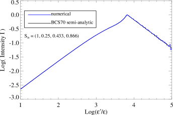
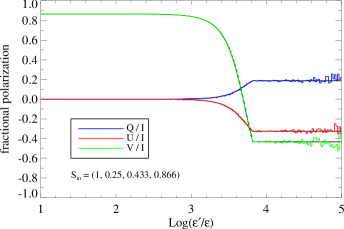
Figure 26.— Same as in Fig. 25, but for $S_{\text{in}}=(1,0.25,0.433,0.866)$.

4.11. Polarized RT with Faraday Rotation and Conversion

In section 3.4 we discussed a scheme to solve the polarized RT with Faraday rotation and conversion incorporated. Now we will test its validation by applying it to solve two RT problems that have analytic solutions presented in Appendix D. Similar tests have been carried out by Dexter (2016) and Mościbrodzka & Gammie (2018) using alternative numerical methods. We emphasize that if there has no scattering in these RT problems, the MC method just provides another choice to solve them and has no any advantages comparing to these numerical methods. The advantage of our method lies in solving the RT with scattering. The results of the two tests are demonstrated in Fig. 27, where the solid and dotted lines represent the analytical and our numerical results, respectively. One can see that they are consistent with each other very well.

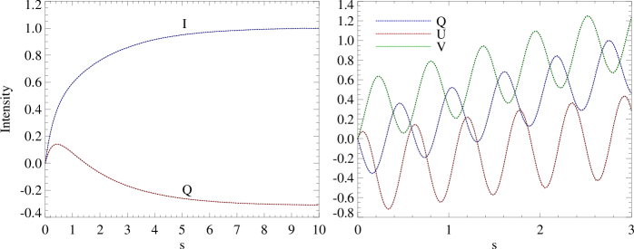
Figure 27.— The tests of MC scheme for RT with Faraday rotation and conversion incorporated against the analytical solutions. Left panel: only the SPs $I$ and $Q$ are involved, and the parameters are: $\alpha_{I}=2.0,\alpha_{Q}=1.5,j_{I}=2.1,j_{Q}=1.2$ and $\alpha=3.0$. Right panel: the Figure illustrates the evolution of SPs $Q$, $U$ and $V$. The parameters are: $\alpha_{IQUV}=0.0,\rho_{Q}=7.5,\rho_{U}=3.4,\rho_{V}=7.2,j_{Q}=-10.717,j_{U}=9.033,\rho_{V}=9.0587$ and $\alpha=200.0$. In the two panels, the solid and dotted lines represent the analytical and MC numerical results, respectively.

5. DISCUSSION

In this paper we have proposed a new MC scheme based on Neumann series solutions of Fredholm integral equations of second kind to solve the RT problems with scattering incorporated. From this perspective, the problem of RT is equivalent to evaluate infinite terms of multiple integrals simultaneously and the MC method is naturally introduced since it has a remarkable efficiency in evaluating multiple integrals. Due to the special structure of Neumann solution, the procedure of integral evaluation amounts to generate random sequences in the phase space. The combination of these sequences with their corresponding weight functions can immediately give the estimations for the observational quantities.

We have reviewed and redescribed the procedure to solve an RTE by the MC method completely and systematically from the perspective of integral equation and its Neumann solution. We particularly emphasize that all complicated and abstract MC sampling algorithms for the transport and scattering of a photon can be understood and explained mathematically. Meanwhile we try to ignore the corresponding physical explanations. Such a treatment not only makes the MC method to be more understandable but also can avert mistakes caused by physical intuitions. Most importantly it enables one to have the flexibility of choosing various sampling PDFs and corresponding weight functions conveniently. These choices are equivalent but with different computational efficiency and accuracy. Particularly the widely adopted conventional photon tracing scheme can be regarded as a special choice, where the PDF for position transport has definitions in the whole space.

We emphasize the importance of recording function which connects the Neumann solution with the observational quantities directly. Especially, any delta function (which is exactly the reason why the photon tracing scheme has a low computational efficiency, since tremendous calculations are inevitably abandoned) contained in the recording function can be eliminated in advance. After that we can choose anther recording function, which enables that any sample in a random sequence can make contribution to the quantity that is under calculation. This estimation strategy can significantly improve the calculation accuracy, especially for systems with axial or spherical symmetry. Usually under the same condition our results have a relatively higher precision comparing to that of the photon tracing scheme. In some ideal situations, the precision is even comparable with the semi-analytical results. But for each estimation, our scheme requires to calculate the recording function and total optical depth from the scattering site to the boundary of the region. It will inevitably occupy additional computational resources.

This new scheme can be directly extended to deal with polarized radiative transfer processes, especially for that the Faraday rotation and conversion effects are incorporated. The polarizations are described by the SPs and the RTEs become a set of differentio-integral equations. The key point is that one should choose common transport PDFs (including position transport and scattering) that is shared by all components of the SPs, meanwhile their updating ways from the incident direction to the scattered direction and estimation functions are different. One of the advantages of our scheme in dealing with the polarized Compton scattering is that we do not have to carry out the Lorentz transformations in terms of SPs between different references. This procedure that involves complicated SPs transformations and rotations (Krawczynski, 2012) now can be avoided.

According to the scheme, a public available MCRT code, named Lemon, has been developed with Fortran. In the development, we find that the Object-Oriented programming is very suitable and convenient to implement our scheme. We first define a basic particle class, which contains the primary members and methods, such as coordinates, momentum, energy, weights, etc.. Then we extend this class gradually by class inheritance and adding new members and methods to the subclass that can implement various special functions. Each extension corresponds one function and the relevant variables and subroutines of which are saved in a single module. These functions include initiating all parameters, starting a sequence, position transport, photon scattering and quantity estimation and so on. As one of the functions is modified, any other will not be affected. Finally we can instantiate these subclasses and obtain different objects. Calling the object’s methods we can generate a scattering sequences and estimate the observational quantity as the generation goes on.

In order to verify the correctness of the scheme and the code, we have reproduced a lot of classic results and made comparisons with them, which have demonstrated the validation and advantages of our scheme. Since the algorithms for sampling various PDFs are crucial for MC method, they have been discussed in detail and the proofs for some of them are also provided in the appendix.

MCRT has an intrinsic parallelization property due to the calculations of random sequences are independent from each other. In order to speed up the calculations, the MPI parallel scheme has been incorporated into the code. In the implementation of parallelization, all of the MPI processes are treated equally, i.e., they are initiated with the same parameters, load the same data files (that contain the tabulated total scattering cross section, the temperature and the electron number density distributions, etc.) and share the same emissivity, scattering and absorption coefficients. Which means that each MPI process requires the access to the full radiating domain. And this requirement can be easily fulfilled for all of our test examples, since they are relatively simple (or the radiating domain can be described semi-analytically) and do not involve any applications to complicated numerical simulations. The sizes of these data files are small and can be easily loaded by each process.

Without any applications to numerical simulations is really the shortage of our code testing. Considering the extreme significance and widely applications of magnetohydrodynamic simulations in nowadays, we really hope that we can apply our code to these simulations in the near future. Numerical simulations with large simulation domains can no longer be load by each process. To overcome these difficulties, new parallelization algorithms and techniques are in desperate needed (e.g., down sampling of the simulation grid and domain decomposition). And the structure of MPI parallelization implemented in the present code should be redesigned completely.

Anther limit of our code testing is that all of the test problems are confined to static configurations. However the fluid flows in numerical simulations usually have large nonuniform velocities that even can be comparable to the speed of light. So can our code handle the RT processes in fluid flow with irregular velocity field consistently? The answer is yes or in principle it can. The procedure can be stated as follows.

First we must choose a global and static reference, since the Neumann solution consists of integrals defined over the entire radiative domain. Such reference obviously exists, in which the velocity field of the fluid flow is also appropriately defined on a grid. Next our scheme requires the mathematical expressions for all relevant quantities of the fluid flow (such as the emissivity, absorption and scattering coefficients, the mass and particle number density, temperature distribution) to be explicitly given in this frame. These quantities are well defined in the comoving (or rest) frame of the fluid flow. So simply through a Lorentz transformation, we can obtain these expressions in the global static frame (one should also notice that in order to get the values of these quantities at an arbitrary position from the simulation data that defined on a grid, a suitable interpolation scheme should be introduced). The Lorentz transformations for these quantities have been extensively studied and can be found in many textbooks (e.g., in the appendix of Pomraning (1973)). With these quantities are specified, we can write down the RTE immediately and obtain the Neumann solution as well. Then the following steps are just routines that have been discussed in the previous sections.

Another problem needs be carefully treated when dealing with RT in optically thick media with our scheme. In this special case, the aforementioned criterion (as the weight of these photons falling below a threshold) to truncate a scattering sequence will become extremely inefficient and therefore should be rejected. The reason can be stated as follow. Since the optically thick region tends to trap any photon that travels into it, the samples of a scattering sequence could be disproportionately distributed over this region. Due to the factor $\exp(-\tau)$ in the recording function, the large optical depth will heavily attenuate the contributions made by these samples to the observed flux. Thus the whole contribution of the sequence is quite low. Meanwhile the evaluation of $\tau$ for each sample is time consuming in optical thick region, especially for post-processing of finite volume simulations with large grids. The situation can be even worse if the weight decreases slowly, such as in cases where the true absorption can be neglected or no absorption exists at all. If we still require the sequence to be truncated as the weight is smaller than the threshold, the scattering times will be a quite large number, which makes the computational cost for evaluating $\tau$ becomes unacceptable. The cost almost offsets the limited gain in the lower variance.

We think the best way to alleviate this difficulty is to truncate the scattering sequence as soon as possible. Once the photon is scattered into high optical depth region, the frequent scattering will trap it and prevent it to escape from the region. Considering the high computational costs and low contributions made by the subsequent samples, we can safely truncate the sequence once the optical depth of a sample is larger than a threshold.

Another useful truncation standard is related to the scattering numbers. For systems with low scattering optical depth, we approximately have $\exp(-\tau_{s})\approx 1+\tau_{s}$ and $A=1-\exp(-\tau_{s})\approx\tau_{s}$, then $I_{m}\propto A_{1}A_{2}\cdots A_{m}\exp(-\tau_{s})\approx\tau_{s}^{m}$, which will decrease rapidly as $m$ increases. So we can truncate the sequence as $m$ is greater than a particular number. For example, from Fig. 18, one can see that the contributions made by photons that have been scattered for more than 4 times can be safely rejected.

In present paper, the discussions are mainly restricted to the classic RT problems in flat spacetime. Our scheme is dependent heavily on the specific forms of RTEs, which should be given explicitly to obtain the Neumann solution and the transport kernel. In curved spacetime, the RTEs are usually given in a covariant form (Younsi et al., 2012; Gammie & Leung, 2012; Bronzwaer et al., 2020), but the scattering incorporated RTEs are rarely provided completely and explicitly, especially for the polarized situations. One exception is in cosmology regime, where in order to study the polarized radiative transfer and perturbations of CMB in the cosmic metrics, the RTEs with polarized Compton scattering have been extensively discussed (Kosowsky, 1996; Portsmouth & Bertschinger, 2004; Weinberg, 2008). For the MCRTs with scattering surround Black holes, instead of writing down the RTEs and starting from the Neumann solutions, one prefers to generate photons and trace them until to the endings (Dolence et al., 2009; Schnittman & Krolik, 2013; Zhang et al., 2019), and the polarizations are usually described by the so-called polarization vectors, which are parallel transported along geodesics. In the future, we hope to extend our scheme from flat to curved spacetime and incorporate it with the results of GRMHD simulations to mimic more real RT processes, which are crucial to interpret the polarized observations generated by accreting black holes.

Finally we want to point out a difference between flat and curved spacetime which may cause difficulties for our scheme. In flat spacetime, once the line of sight of the observer, $\mathbf{\Omega}_{\text{obs}}$, is provided, the scattered direction $\mathbf{\Omega}^{\prime}$ in the scattering kernel $C(\nu,\mathbf{\Omega}\rightarrow\nu^{\prime},\mathbf{\Omega}^{\prime})$ can be replaced by $\mathbf{\Omega}_{\text{obs}}$ directly and $C(\nu,\mathbf{\Omega}\rightarrow\nu^{\prime},\mathbf{\Omega}_{\text{obs}})$ will be taken as a weight for estimations. While in curved spacetime, due to the light bending, we can not carry out such a replacement anymore, unless we determine the geodesic connecting the observer and the scattering point and then $\mathbf{\Omega}^{\prime}$ should be replaced by the unit tangent vector of the geodesic at the scattering point rather than $\mathbf{\Omega}_{\text{obs}}$. It implies that for each estimation of our scheme in curved spacetime, a geodesic with two fixed points (i.e., observer at infinity and the scattering point) needs be determined additionally. Fortunately, some excellent codes already exist for computing the photon geodesics in curved spacetime. Especially the public available code geokerr (Dexter & Agol, 2009) can compute the geodesics between two points in Kerr metric, even without full integrations.

Appendix A the proof of the algorithm for position transport

Here we present a proof for Algorithm 3 that randomly generates a scattering distance $s$. What we need to prove is that the probability $p(s)$ for a sample $s$ is selected by this algorithm is proportional to $\sigma_{s}(s)\exp\left(-\int_{0}^{s}\sigma_{s}(l)dl\right)$, where $\sigma_{s}(s)=\sigma_{s}(\mathbf{r}+s\mathbf{\Omega},\nu,\mathbf{\Omega})$ is the scattering coefficient. According to the algorithm, we know that an $s$ can be expressed as the sum of $s_{i}$: $s=s_{1}+s_{2}+\cdots+s_{n}$, where $n=1,2,\cdots$, and $s_{i}$ are samples of a random variable $l$ with the PDF given by $\displaystyle\widetilde{p}_{1}(l)=\sigma_{\text{max}}\exp(-\sigma_{\text{max}}l)/N,\,0\leq l\leq s_{\text{max}}$, and $N=1-\exp(-\sigma_{\text{max}}s_{\text{max}})$ is the normalization factor. Suppose $p_{n}(s)$ is the probability that the $s_{i}$ ($i=1,\cdots,n$) are generated and their sum is accepted as a sample of $s$. Then the total probability corresponding an $s$ is selected can be expressed as

$$p(s)=\sum^{\infty}_{n=1}p_{n}(s).$$ (A1)

Obviously for $n=1$, we have

$$\displaystyle p_{1}(s)=\widetilde{p}_{1}(s)\frac{\sigma_{s}(s)}{\sigma_{\text{max}}}=\frac{\sigma_{s}(s)}{N}\exp(-\sigma_{\text{max}}s).$$ (A2)

As $n=2$, we have $s=s_{1}+s_{2}$, and the probability of generating $s_{1},s_{2}$ by sampling $\widetilde{p}_{1}(l)$ and accepting them can be written as

$$\begin{split}&p(s_{1})\displaystyle=\widetilde{p}_{1}(s_{1})\left(1-\frac{\sigma_{s}(s_{1})}{\sigma_{\text{max}}}\right)\widetilde{p}_{1}(s_{2})\frac{\sigma_{s}(s_{1}+s_{2})}{\sigma_{\text{max}}}N\displaystyle=\frac{\sigma_{s}(s)}{N}\exp(-\sigma_{\text{max}}s)[\sigma_{\text{max}}-\sigma_{s}(s_{1})].\end{split}$$ (A3)

Notice that $s_{1}$ can actually take any value on interval $(0,s)$ and each value corresponds a probability $p(s_{1})$, thus the total probability should be

$$\displaystyle p_{2}(s)=\int_{0}^{s}p(s_{1})ds_{1}=\frac{\sigma_{s}(s)}{N}\exp(-\sigma_{\text{max}}s)\int_{0}^{s}[\sigma_{\text{max}}-\sigma_{s}(s_{1})]ds_{1}.$$ (A4)

Similarly, for $n=3$, we have

$$\begin{split}p(s_{1},s_{2})&\displaystyle=\widetilde{p}_{1}(s_{1})\left(1-\frac{\sigma_{s}(s_{1})}{\sigma_{\text{max}}}\right)\widetilde{p}_{1}(s_{2})\left(1-\frac{\sigma_{s}(s_{1}+s_{2})}{\sigma_{\text{max}}}\right)N\widetilde{p}_{1}(s_{3})\frac{\sigma_{s}(s)}{\sigma_{\text{max}}}N\\ &\displaystyle=\frac{\sigma_{s}(s)}{N}\exp(-\sigma_{\text{max}}s)[\sigma_{\text{max}}-\sigma_{s}(s_{1})][\sigma_{\text{max}}-\sigma_{s}(s_{1}+s_{2})].\end{split}$$ (A5)

Notice that $s_{1}$ can also take any value on interval $(0,s)$ and $s_{2}$ on $(0,s-s_{1})$, thus we have

$$\begin{split}&p_{3}(s)\displaystyle=\int_{0}^{s}ds_{1}\int_{0}^{s-s_{1}}ds_{2}p(s_{1},s_{2})=\frac{\sigma_{s}(s)}{N}\exp(-\sigma_{\text{max}}s)\int_{0}^{s}ds_{1}\int_{0}^{s-s_{1}}ds_{2}[\sigma_{\text{max}}-\sigma_{s}(s_{1})][\sigma_{\text{max}}-\sigma_{s}(s_{1}+s_{2})].\end{split}$$ (A6)

Then the expression for $p_{n}(s)$ can be obtained directly as

$$\begin{split}&p_{n}(s)\displaystyle=\frac{\sigma_{s}(s)}{N}\exp(-\sigma_{\text{max}}s)\int_{0}^{s}ds_{1}\int_{0}^{s-s_{1}}ds_{2}\cdots\int_{0}^{s-(s_{1}+\cdots+s_{n-2})}ds_{n-1}f(s_{1})f(s_{1}+s_{2})\cdots f(s_{1}+\cdots+s_{n-1}),\end{split}$$ (A7)

where $f(s)=\sigma_{\text{max}}-\sigma(s)$. We introduce a set of new variables $y_{1},\cdots,y_{n-1}$ defined by

$$y_{1}=s_{1},\,\,\,\,y_{2}=s_{1}+s_{2},\,\,\,\,\cdots,\,\,\,\,y_{n-1}=s_{1}+\cdots+s_{n-1},$$ (A8)

we have $s_{1}=y_{1},\,\,s_{2}=y_{2}-y_{1},\,\,\cdots,\,\,s_{n-1}=y_{n-1}-y_{n-2}$. One can easily show that the Jacobian of this transformation is $J=\left|\partial(s_{1},\cdots,s_{n-1})/\partial(y_{1},\cdots,y_{n-1})\right|=1$. So the volume element is unchanged, i.e., $dy_{1}dy_{2}\cdots dy_{n-1}=ds_{1}ds_{2}\cdots ds_{n-1}$. Then $p_{n}(s)$ can be rewritten as

$$p_{n}(s)\displaystyle=\frac{\sigma_{s}(s)}{N}\exp(-\sigma_{\text{max}}s)\int_{0}^{s}dy_{1}\int_{y_{1}}^{s}dy_{2}\cdots\int_{y_{n-2}}^{s}dy_{n-1}f(y_{1})f(y_{2})\cdots f(y_{n-1}).$$ (A9)

Notice that

$$\int_{0}^{s}dy_{1}\int_{y_{1}}^{s}dy_{2}\cdots\int_{y_{n-2}}^{s}dy_{n-1}f(y_{1})\cdots f(y_{n-1})=\frac{1}{(n-1)!}\left[\int_{0}^{s}f(y)dy\right]^{n-1},$$ (A10)

we have

$$p_{n}(s)\displaystyle=\frac{\sigma_{s}(s)}{N}\exp(-\sigma_{\text{max}}s)\frac{1}{(n-1)!}\left[\int_{0}^{s}[\sigma_{\text{max}}-\sigma_{s}(y)]dy\right]^{n-1}.$$ (A11)

Eventually we arrive at

$$\begin{split}p(s)&=\sum_{n=1}^{\infty}p_{n}(s)=\frac{\sigma_{s}(s)}{N}\exp(-\sigma_{\text{max}}s)\sum_{n=1}^{\infty}\frac{1}{(n-1)!}\left[\int_{0}^{s}[\sigma_{\text{max}}-\sigma_{s}(y)]dy\right]^{n-1}\\ &=\frac{\sigma_{s}(s)}{N}\exp(-\sigma_{\text{max}}s)\exp\left[\sigma_{\text{max}}s-\int_{0}^{s}\sigma_{s}(y)dy\right]=\frac{\sigma_{s}(s)}{N}\exp\left[-\int_{0}^{s}\sigma_{s}(y)dy\right],\end{split}$$ (A12)

i.e., $p(s)\propto\sigma_{s}(s)\exp\left(-\int_{0}^{s}\sigma_{s}(l)dl\right)$.

Appendix B The Sampling Algorithm For PDFs with Triangular functions

When dealing with scattering processes, one often encounters PDFs that consist of triangular functions, for example $p(\varphi)=a_{0}+a_{1}\cos\varphi+a_{2}\cos 2\varphi+b_{1}\sin\varphi+b_{2}\sin 2\varphi$. If one uses the inverse CDF method to sample such an PDF, a transcendental equation which is analogous to Kepler equation but more complicated needs to be solved. However, we can construct a new algorithm that utilizes the properties of piecewise central symmetry and the odd and even of triangular functions to sample a more general triangular function PDF $p(\varphi)$ given by

$$p(\varphi)=a_{0}+\sum_{m=1}^{M}a_{m}\cos m\varphi+\sum_{n=1}^{N}b_{n}\sin n\varphi,$$ (B1)

where $M$ and $N$ can be any positive integers, the coefficients $a_{i}$ and $b_{i}$ are given in a way that $p(\varphi)$ is always positive. We introduce some new constants defined as

$$p_{m}=\frac{|a_{m}|}{a_{0}},\quad p_{0}=\displaystyle 1-\sum_{m=1}^{M}p_{m},\quad\displaystyle P_{m}=\sum_{i=0}^{m}p_{i},$$ (B2)

which satisfy the conditions: $0\leq p_{i}<1$ and $p_{0}+p_{1}+\cdots+p_{M}=1$. Then $p(\varphi)$ can be recast as

$$p(\varphi)=F(\varphi)+H(\varphi),$$ (B3)

where

$$\displaystyle F(\varphi)=a_{0}\left[p_{0}+\sum_{m=1}^{M}p_{m}(1+s_{m}\cos m\varphi)\right],\quad\displaystyle H(\varphi)=\sum_{n=1}^{N}b_{n}\sin n\varphi,$$ (B4)

and $s_{m}=\text{sign}(a_{m})$. The sampling procedure of $p(\varphi)$ is provided in Algorithm. 4, where $\xi_{i}$ are random numbers, $n=[\varphi_{t}/(\pi/m)]$ and $[x]$ represents the function that gets the maximum integer that is smaller than $x$. A test example of this algorithm is given in Fig. 28.

① Let $\varphi_{t}=2\pi\cdot\xi_{1}$

if $\left(\displaystyle 0\leq\xi_{2}<P_{0}\right)$ then

       $\varphi_{\xi}=\varphi_{t}$

else if $\left(\displaystyle P_{m-1}\leq\xi_{2}<P_{m}\right)$ then

       if $2\xi_{3}\leq 1+s_{m}\cos m\varphi$ then

             $\varphi_{\xi}=\varphi_{t}$

      else

            $\varphi_{\xi}=(2n+1)\pi/m-\varphi_{t}$

      

if $\left(\displaystyle\xi_{4}-1\leq\frac{H(\varphi_{\xi})}{F(\varphi_{\xi})}\right)$ then

      $\quad\varphi=\varphi_{\xi}$

else

      $\varphi=2\pi-\varphi_{\xi}$

Algorithm 4 Triangular PDF Sampling Algorithm

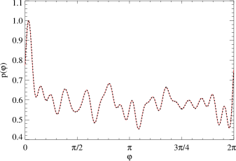
Figure 28.— A testing example of Algorithm. 4 for sampling a PDF given by Eq. (B1). The coefficients $a_{i}$ and $b_{i}$ are all random numbers and $M=40,\,N=30$. The function $p(\varphi)$ is plotted in red solid line, while the normalized sample numbers generated by the algorithm is plotted in black dotted line.

Appendix C The Sampling Procedures For Rayleigh’s Scattering matrix in a static frame

In section 4.5, we discussed the angular dependent SPs of radiations that are diffusely reflected from a plane-parallel semi-infinite atmosphere. The equations describing the RT in such a system are given by Eqs. (129), in which the Rayleigh’s scattering matrix $\mathbf{P}$ is given by (Eqs. (220)-(224) of (Chandrasekhar, 1960) Chap. I, page 42)

$$\displaystyle\mathbf{P}(\mu,\varphi;\mu^{\prime},\varphi^{\prime})=\mathbf{Q}[\mathbf{P}^{(0)}(\mu,\mu^{\prime})+\sqrt{1-\mu^{2}}\sqrt{1-\mu^{\prime 2}}\mathbf{P}^{(1)}(\mu,\varphi;\mu^{\prime},\varphi^{\prime})+\mathbf{P}^{(2)}(\mu,\varphi;\mu^{\prime},\varphi^{\prime})],$$ (C1)

where

$$\displaystyle\mathbf{Q}=\left(\begin{array}[]{cccc}\displaystyle 1&\quad 0&\quad 0&\quad 0\\ \displaystyle 0&\quad 1&\quad 0&\quad 0\\ \displaystyle 0&\quad 0&\quad 2&\quad 0\\ \displaystyle 0&\quad 0&\quad 0&\quad 2\\ \end{array}\right),\quad\quad\displaystyle\mathbf{P}^{(0)}(\mu,\mu^{\prime})=\frac{3}{4}\left(\begin{array}[]{cccc}\displaystyle 2(1-\mu^{2})(1-\mu^{\prime 2})+\mu^{2}\mu^{\prime 2}&\quad\mu^{2}&\quad 0&\quad 0\\ \displaystyle\mu^{\prime 2}&\quad 1&\quad 0&\quad 0\\ \displaystyle 0&\quad 0&\quad 0&\quad 0\\ \displaystyle 0&\quad 0&\quad 0&\quad\mu\mu^{\prime}\\ \end{array}\right),$$ (C10)

$$\displaystyle\mathbf{P}^{(1)}(\mu,\varphi;\mu^{\prime},\varphi^{\prime})=\frac{3}{4}\left(\begin{array}[]{cccc}\displaystyle 4\mu\mu^{\prime}\cos(\varphi^{\prime}-\varphi)&\quad 0&\quad 2\mu\sin(\varphi^{\prime}-\varphi)&\quad 0\\ \displaystyle 0&\quad 0&\quad 0&\quad 0\\ \displaystyle-2\mu^{\prime}\sin(\varphi^{\prime}-\varphi)&\quad 0&\quad\cos(\varphi^{\prime}-\varphi)&\quad 0\\ \displaystyle 0&\quad 0&\quad 0&\quad\cos(\varphi^{\prime}-\varphi)\\ \end{array}\right),$$ (C15)

$$\displaystyle\mathbf{P}^{(2)}(\mu,\varphi;\mu^{\prime},\varphi^{\prime})=\frac{3}{4}\left(\begin{array}[]{cccc}\displaystyle\mu^{2}\mu^{\prime 2}\cos 2(\varphi^{\prime}-\varphi)&\quad-\mu^{2}\cos 2(\varphi^{\prime}-\varphi)&\quad\mu^{2}\mu^{\prime}\sin 2(\varphi^{\prime}-\varphi)&\quad 0\\ \displaystyle-\mu^{\prime 2}\cos 2(\varphi^{\prime}-\varphi)&\quad\cos 2(\varphi^{\prime}-\varphi)&\quad-\mu^{\prime}\sin 2(\varphi^{\prime}-\varphi)&\quad 0\\ \displaystyle-\mu\mu^{\prime 2}\sin 2(\varphi^{\prime}-\varphi)&\quad\mu\sin 2(\varphi^{\prime}-\varphi)&\quad\mu\mu^{\prime}\cos 2(\varphi^{\prime}-\varphi)&\quad 0\\ \displaystyle 0&\quad 0&\quad 0&\quad 0\\ \end{array}\right).$$ (C20)

Notice that the above matrices are defined with respect to SPs $I_{l},I_{r},U,V$ rather than $I,Q,U,V$. In MCRT, we prefer to use $I,Q,U,V$ to describe the polarizations instead, so we need to make a transformation to get a new matrix $\widetilde{\mathbf{P}}$ that is defined in terms of $I,Q,U,V$. One can show that the elements of the new matrix are given by

$$\left\{\begin{array}[]{llll}\displaystyle\widetilde{P}_{11}=(P_{11}+P_{12}+P_{21}+P_{22})/2,&\quad\widetilde{P}_{12}=(P_{11}-P_{12}+P_{21}-P_{22})/2,&\quad\widetilde{P}_{13}=P_{13}+P_{23},&\quad\widetilde{P}_{14}=0,\\ \displaystyle\widetilde{P}_{21}=(P_{11}+P_{12}-P_{21}-P_{22})/2,&\quad\widetilde{P}_{22}=(P_{11}-P_{12}-P_{21}+P_{22})/2,&\quad\widetilde{P}_{23}=P_{13}-P_{23},&\quad\widetilde{P}_{24}=0,\\ \displaystyle\widetilde{P}_{31}=(P_{31}+P_{32})/2,&\quad\widetilde{P}_{32}=(P_{31}-P_{32})/2,&\quad\widetilde{P}_{33}=P_{33},&\quad\widetilde{P}_{34}=0,\\ \widetilde{P}_{41}=0,&\quad\widetilde{P}_{42}=0,&\quad\widetilde{P}_{43}=0,&\quad\widetilde{P}_{44}=P_{44}.\end{array}\right.$$ (C25)

The updating relationship for the quantity $\mathbf{\Psi}=(\Psi^{(I)},\Psi^{(Q)},\Psi^{(U)},\Psi^{(V)})^{T}$ from $m$ to $m+1$ can be obtained directly by multiplying $\mathbf{\Psi}$ with $\widetilde{\mathbf{P}}$ from the left side, i.e.,

$$\left.\begin{array}[]{ll}\displaystyle\Psi^{(I)}_{m+1}=\widetilde{P}_{11}\Psi^{(I)}_{m}+\widetilde{P}_{12}\Psi^{(Q)}_{m}+\widetilde{P}_{13}\Psi^{(U)}_{m},&\displaystyle\Psi^{(Q)}_{m+1}=\widetilde{P}_{21}\Psi^{(I)}_{m}+\widetilde{P}_{22}\Psi^{(Q)}_{m}+\widetilde{P}_{23}\Psi^{(U)}_{m},\\ \displaystyle\Psi^{(U)}_{m+1}=\widetilde{P}_{31}\Psi^{(I)}_{m}+\widetilde{P}_{32}\Psi^{(Q)}_{m}+\widetilde{P}_{33}\Psi^{(U)}_{m},&\displaystyle\Psi^{(V)}_{m+1}=\widetilde{P}_{44}\Psi^{(V)}_{m}.\end{array}\right.$$ (C28)

Or in a more compact form

$$\begin{array}[]{ll}\displaystyle\Psi^{(I)}_{m+1}=f_{I}(\mu,\varphi;\mu^{\prime},\varphi^{\prime})\Psi^{(I)}_{m},&\displaystyle\Psi^{(Q)}_{m+1}=f_{Q}(\mu,\varphi;\mu^{\prime},\varphi^{\prime})\Psi^{(I)}_{m},\\ \displaystyle\Psi^{(U)}_{m+1}=f_{U}(\mu,\varphi;\mu^{\prime},\varphi^{\prime})\Psi^{(I)}_{m},&\displaystyle\Psi^{(V)}_{m+1}=f_{V}(\mu,\varphi;\mu^{\prime},\varphi^{\prime})\Psi^{(V)}_{m},\end{array}$$ (C31)

where

$$\left\{\begin{array}[]{ll}f_{I}(\mu,\varphi;\mu^{\prime},\varphi^{\prime})=&\displaystyle\frac{3}{32\pi}\left[2(1-\mu^{2})(1-\mu^{\prime 2})(1+Q_{m})+(1+\mu^{2})(1+\mu^{\prime 2}-(1-\mu^{\prime 2})Q_{m})\right.\\ &\displaystyle+4\mu\mu^{\prime}\sqrt{1-\mu^{2}}\sqrt{1-\mu^{\prime 2}}(1+Q_{m})\cos(\varphi^{\prime}-\varphi)+4\mu\sqrt{1-\mu^{2}}\sqrt{1-\mu^{\prime 2}}U_{m}\sin(\varphi^{\prime}-\varphi)\\ &\left.+(1-\mu^{2})(1-\mu^{\prime 2})-(1-\mu^{2})(1+\mu^{\prime 2})Q_{m}\cos 2(\varphi^{\prime}-\varphi)-2(1-\mu^{2})\mu^{\prime}U_{m}\sin 2(\varphi^{\prime}-\varphi)\right],\\ f_{Q}(\mu,\varphi;\mu^{\prime},\varphi^{\prime})=&\displaystyle\frac{3}{32\pi}[(1-\mu^{2})(1-\mu^{\prime 2})(2+3Q_{m})-(1-\mu^{2})(1+\mu^{\prime 2})+4\mu\sqrt{1-\mu^{2}}\sqrt{1-\mu^{\prime 2}}U_{m}\sin(\varphi^{\prime}-\varphi)\\ &+4\mu\mu^{\prime}\sqrt{1-\mu^{2}}\sqrt{1-\mu^{\prime 2}}(1+Q_{m})\cos(\varphi^{\prime}-\varphi)\\ &+(1+\mu^{2})(\mu^{\prime 2}-1+(1+\mu^{\prime 2})Q_{m})\cos 2(\varphi^{\prime}-\varphi)+2(1+\mu^{2})\mu^{\prime}\sin 2(\varphi^{\prime}-\varphi)],\\ f_{U}(\mu,\varphi;\mu^{\prime},\varphi^{\prime})=&\displaystyle\frac{3}{32\pi}[4\sqrt{1-\mu^{2}}\sqrt{1-\mu^{\prime 2}}U_{m}\cos(\varphi^{\prime}-\varphi)-4\mu^{\prime}(1+Q_{m}\mu)\sin(\varphi^{\prime}-\varphi)\\ &+2\mu\mu^{\prime}U_{m}\cos 2(\varphi^{\prime}-\varphi)-2\mu(1+\mu^{\prime 2}(1+Q_{m}))\sin 2(\varphi^{\prime}-\varphi)],\\ f_{V}(\mu,\varphi;\mu^{\prime},\varphi^{\prime})=&\displaystyle\frac{3}{8\pi}[\mu\mu^{\prime}+\sqrt{1-\mu^{2}}\sqrt{1-\mu^{\prime 2}}\cos 2(\varphi^{\prime}-\varphi)],\end{array}\right.$$ (C41)

and $Q_{m}=\Psi^{(Q)}_{m}/\Psi^{(I)}_{m}$ and $U_{m}=\Psi^{(U)}_{m}/\Psi^{(I)}_{m}$. As aforementioned in the Section. 3.3, we will take $f_{I}(\mu,\varphi;\mu^{\prime},\varphi^{\prime})$ as the PDF to sample the scattered direction $(\mu,\varphi)$ when the incident direction $(\mu^{\prime},\varphi^{\prime})$ are provided. We can recast it into a more compact form given as follows

$$\displaystyle f_{I}(\mu,\varphi;\mu^{\prime},\varphi^{\prime})=\frac{3}{32\pi}(f_{1}+g_{2}\cos\varphi+g_{3}\sin\varphi+g_{4}\cos 2\varphi+g_{5}\sin 2\varphi),$$ (C42)

where

$$\left\{\begin{array}[]{l }\displaystyle f_{1}(\mu,\mu^{\prime})=2(1-\mu^{2})(1-\mu^{\prime 2})(1+Q_{m})+(1+\mu^{2})[1+\mu^{\prime 2}-(1-\mu^{\prime 2})Q_{m}],\\ \displaystyle f_{2}(\mu,\mu^{\prime})=4\mu\mu^{\prime}\sqrt{1-\mu^{2}}\sqrt{1-\mu^{\prime 2}}(1+Q_{m}),\\ \displaystyle f_{3}(\mu,\mu^{\prime})=4\mu\sqrt{1-\mu^{2}}\sqrt{1-\mu^{\prime 2}}U_{m},\\ \displaystyle f_{4}(\mu,\mu^{\prime})=(1-\mu^{2})(1-\mu^{\prime 2})-(1-\mu^{2})(1+\mu^{\prime 2})Q_{m},\\ \displaystyle f_{5}(\mu,\mu^{\prime})=-2(1-\mu^{2})\mu^{\prime}U_{m},\\ \displaystyle g_{2}=f_{2}\cos\varphi^{\prime}+f_{3}\sin\varphi^{\prime},\quad\quad\quad g_{3}=f_{2}\sin\varphi^{\prime}-f_{3}\cos\varphi^{\prime},\\ \displaystyle g_{4}=f_{4}\cos 2\varphi^{\prime}+f_{5}\sin 2\varphi^{\prime},\quad\quad g_{5}=f_{4}\sin 2\varphi^{\prime}-f_{5}\cos 2\varphi^{\prime}.\end{array}\right.$$ (C50)

Then one can readily show that PDF $p(\mu,\varphi)=f_{I}(\mu,\varphi;\mu^{\prime},\varphi^{\prime})$ is automatically normalized. Integrating out $p(\mu,\varphi)$ over $\varphi$, we get the marginal PDF of $\mu$ as

$$\begin{array}[]{l}\displaystyle p(\mu)=\int_{0}^{2\pi}p(\mu,\varphi)d\varphi=\frac{3}{16}f_{1}(\mu,\mu^{\prime})=\frac{3}{16}(c_{1}\mu^{2}+c_{2}),\end{array}$$ (C52)

where $c_{1}=1+\mu^{\prime 2}-(1-\mu^{\prime 2})Q_{m}-2(1-\mu^{\prime 2})(1+Q_{m})$ and $c_{2}=1+\mu^{\prime 2}-(1-\mu^{\prime 2})Q_{m}+2(1-\mu^{\prime 2})(1+Q_{m})$. Hence we can use the inverse CDF method to get the scattered $\mu$, which is the real root of the equation $c_{1}\mu^{3}+3c_{2}\mu+c_{1}+3c_{2}-16\xi=0$ on interval $[-1,1]$, where $\xi$ is a random number. When $\mu$ is obtained, we can immediately get the PDF for $\varphi$ by using the Bayes formula $p(\varphi|\mu)=p(\mu,\varphi)/p(\mu)$ as

$$\displaystyle p(\varphi|\mu)=\frac{1}{2\pi f_{1}}(f_{1}+g_{2}\cos\varphi+g_{3}\sin\varphi+g_{4}\cos 2\varphi+g_{5}\sin 2\varphi).$$ (C53)

Now the inverse CDF method seems unfeasible to sample $p(\varphi|\mu)$, since it will give rise to a transcendental equation in terms of $\varphi$ and more complicated than the Kepler equation. But utilizing the symmetrical and periodic properties of triangular functions, we have constructed an Algorithm. 4 that can circumvent this difficulty. In order to sample $p(\varphi|\mu)$ through Algorithm. 4, we introduce some relevant quantities given by

$$\begin{array}[]{l}\displaystyle F(\varphi)=\frac{1}{2\pi f_{1}}(f_{1}+g_{2}\cos\varphi+g_{4}\cos 2\varphi),\quad H(\varphi)=\frac{1}{2\pi f_{1}}(g_{3}\sin\varphi+g_{5}\sin 2\varphi),\\ \displaystyle p_{0}=1-p_{1}-p_{2},\quad p_{1}=\frac{|g_{2}|}{f_{1}},\quad p_{2}=\frac{|g_{4}|}{f_{1}},\quad s_{1}=\text{sign}(g_{2}),\quad s_{2}=\text{sign}(g_{4}).\end{array}$$ (C56)

With $\mu$ and $\varphi$ are obtained, we can simply update the components of scattered $\mathbf{\Psi}$ as

$$\begin{array}[]{ll}\displaystyle\Psi^{(I)}_{m+1}=\Psi^{(I)}_{m},&\displaystyle\Psi^{(Q)}_{m+1}=\frac{f_{Q}(\mu,\varphi;\mu^{\prime},\varphi^{\prime})}{f_{I}(\mu,\varphi;\mu^{\prime},\varphi^{\prime})}\Psi^{(I)}_{m},\\ \displaystyle\Psi^{(U)}_{m+1}=\frac{f_{U}(\mu,\varphi;\mu^{\prime},\varphi^{\prime})}{f_{I}(\mu,\varphi;\mu^{\prime},\varphi^{\prime})}\Psi^{(I)}_{m},&\displaystyle\Psi^{(V)}_{m+1}=\frac{f_{V}(\mu,\varphi;\mu^{\prime},\varphi^{\prime})}{f_{I}(\mu,\varphi;\mu^{\prime},\varphi^{\prime})}\Psi^{(V)}_{m}.\end{array}$$ (C59)

Appendix D The Analytic Solutions for RT equations with Faraday Rotation and Conversion

Now we give the analytical solutions for two RT problems including Faraday effects. In the first case, only the $j_{IQ}$ and $\alpha_{IQ}$ are presented and the RTE reads as

$$\begin{split}\frac{d}{ds}\begin{pmatrix}I\\ Q\end{pmatrix}=\begin{pmatrix}j_{I}\\ j_{Q}\end{pmatrix}-\begin{pmatrix}\alpha_{I}&\alpha_{Q}\\ \alpha_{Q}&\alpha_{I}\end{pmatrix}\begin{pmatrix}I\\ Q\end{pmatrix},\end{split}$$ (D1)

the analytic solution of which can be written as

$$\begin{split}I(s)=\frac{j_{+}}{2\alpha_{+}}(1-\text{e}^{-\alpha_{+}s})+\frac{j_{-}}{2\alpha_{-}}(1-\text{e}^{-\alpha_{-}s})+\frac{1}{2}\text{e}^{-\alpha_{+}s}(I_{0}+Q_{0})+\frac{1}{2}\text{e}^{-\alpha_{-}s}(I_{0}-Q_{0}),\\ Q(s)=\frac{j_{+}}{2\alpha_{+}}(1-\text{e}^{-\alpha_{+}s})-\frac{j_{-}}{2\alpha_{-}}(1-\text{e}^{-\alpha_{-}s})+\frac{1}{2}\text{e}^{-\alpha_{+}s}(I_{0}+Q_{0})-\frac{1}{2}\text{e}^{-\alpha_{-}s}(I_{0}-Q_{0}),\end{split}$$ (D2)

where $j_{\pm}=j_{I}\pm j_{Q}$, $\alpha_{\pm}=\alpha_{I}\pm\alpha_{Q}$, and $I_{0},Q_{0}$ are the initial values of $I$ and $Q$ at $s=0$. In the second case, all of the absorption coefficients $\alpha_{IQUV}$ and emissivity $j_{I}$ vanish, the RTE can be written as

$$\frac{d}{ds}\begin{pmatrix}Q\\ U\\ V\end{pmatrix}=\begin{pmatrix}j_{Q}\\ j_{U}\\ j_{V}\end{pmatrix}-\begin{pmatrix}0&\rho_{V}&-\rho_{U}\\ -\rho_{V}&0&\rho_{Q}\\ \rho_{U}&-\rho_{Q}&0\\ \end{pmatrix}\begin{pmatrix}Q\\ U\\ V\end{pmatrix}.$$ (D3)

Integrating the above equations directly, we have (Mościbrodzka & Gammie, 2018)

$$\left\{\begin{split}Q(s)=&\frac{\rho_{Q}}{\rho^{2}}\rho\cdot\boldsymbol{J}s+(j_{Q}\rho^{2}-\rho_{Q}\rho\cdot\boldsymbol{J})\frac{\sin(\rho s)}{\rho^{3}}+(\rho_{U}j_{V}-\rho_{V}j_{U})\frac{1-\cos(\rho s)}{\rho^{2}}\\ &+Q_{0}\cos(\rho s)+2\frac{\rho_{Q}(\rho\cdot\boldsymbol{S})}{\rho^{2}}\sin^{2}(\rho s/2)+\frac{\rho_{U}V_{0}-\rho_{V}U_{0}}{\rho}\sin(\rho s),\\ U(s)=&\frac{\rho_{U}}{\rho^{2}}\rho\cdot\boldsymbol{J}s+(j_{U}\rho^{2}-\rho_{U}\rho\cdot\boldsymbol{J})\frac{\sin(\rho s)}{\rho^{3}}+(\rho_{V}j_{Q}-\rho_{Q}j_{V})\frac{1-\cos(\rho s)}{\rho^{2}}\\ &+U_{0}\cos(\rho s)+2\frac{\rho_{U}(\rho\cdot\boldsymbol{S})}{\rho^{2}}\sin^{2}(\rho s/2)+\frac{\rho_{V}Q_{0}-\rho_{Q}V_{0}}{\rho}\sin(\rho s),\\ V(s)=&\frac{\rho_{V}}{\rho^{2}}\rho\cdot\boldsymbol{J}s+(j_{V}\rho^{2}-\rho_{V}\rho\cdot\boldsymbol{J})\frac{\sin(\rho s)}{\rho^{3}}+(\rho_{Q}j_{U}-\rho_{U}j_{Q})\frac{1-\cos(\rho s)}{\rho^{2}}\\ &+V_{0}\cos(\rho s)+2\frac{\rho_{V}(\rho\cdot\boldsymbol{S})}{\rho^{2}}\sin^{2}(\rho s/2)+\frac{\rho_{Q}U_{0}-\rho_{U}Q_{0}}{\rho}\sin(\rho s),\end{split}\right.$$ (D4)

where $\rho^{2}=\rho_{Q}^{2}+\rho_{U}^{2}+\rho_{V}^{2}$, $\rho\cdot\boldsymbol{S}=\rho_{Q}Q_{0}+\rho_{U}U_{0}+\rho_{V}V_{0}$, $\mathbf{\rho}\cdot\boldsymbol{J}=\rho_{Q}j_{Q}+\rho_{U}j_{U}+\rho_{V}j_{V}$, and $Q_{0},U_{0},V_{0}$ are the initial values of $Q,U,V$ at $s=0$.

Appendix E The Neumann solution as the disk reflection effect considered

Now we discuss what should the sampling procedure be modified when the reflection term $\mathbf{I}_{r}$ given by Eq. (151) is incorporated. Although the discussion is presented in a plane-parallel geometrical system, it is possible to extend it to any other systems. Since the reflected radiations can reenter the corona, they can be regarded as the seed photons that will initiate another round of RT process. It means that the RT problem now becomes an iterative one. Assume that $\mathbf{J}(\tau_{0},\mathbf{\Omega},\nu)$ is the primary radiations emitted by the disk, the corresponding radiative flux generated by $\mathbf{J}$ is $\mathbf{\Psi}^{(0)}$, which obviously satisfies the integral equation

$$\begin{split}&\mathbf{\Psi}^{(0)}(P)=\mathbf{J}(P)+\int\mathbf{K}(P^{\prime}\rightarrow P)\mathbf{\Psi}^{(0)}(P^{\prime})dP^{\prime}.\end{split}$$ (E1)

Their Neumann solutions are

$$\begin{split}&\mathbf{\Psi}^{(0)}(P)=\sum_{m=0}^{\infty}\mathbf{\Psi}^{(0)}_{m}(P),\quad\mathbf{\Psi}^{(0)}_{0}(P)=\mathbf{J}(P),\quad\mathbf{\Psi}^{(0)}_{1}(P)=\int\mathbf{K}(P^{\prime}\rightarrow P)\mathbf{J}(P^{\prime})dP^{\prime}=\mathbf{J}\mathbf{K},\cdots,\\ &\mathbf{\Psi}^{(0)}_{m}(P)=\int\mathbf{K}(P_{m-1}\rightarrow P)\mathbf{K}(P_{m-2}\rightarrow P_{m-1})\cdots\mathbf{K}(P_{0}\rightarrow P_{1})\mathbf{J}(P_{1})dP_{0}\cdots dP_{m-1}=\mathbf{J}\mathbf{K}\cdots\mathbf{K}=\mathbf{J}\mathbf{K}^{m}.\end{split}$$ (E2)

For simplicity, we denote the multiple integrals in terms of any $P$ in a compact form. Using $\mathbf{\Psi}^{(0)}$, we can immediately obtain the radiations escaped from the up and down surfaces of the corona respectively as

$$\begin{split}\begin{array}[]{lr}\displaystyle\mathbf{I}^{(0)}_{\text{up}}(0,\mathbf{\Omega}^{\prime},\nu^{\prime})=\sum_{m=0}^{\infty}\mathbf{I}^{(0)}_{\text{up},m}=\sum_{m=0}^{\infty}\int_{0}^{\tau_{0}}\mathbf{J}\mathbf{K}^{m}\exp\left(-\frac{\tau^{\prime}}{\mu^{\prime}}\right)\frac{d\tau^{\prime}}{\mu^{\prime}},&\quad\mu^{\prime}>0,\\ \displaystyle\mathbf{I}^{(0)}_{\text{dw}}(\tau_{0},\mathbf{\Omega}^{\prime},\nu^{\prime})=\sum_{m=0}^{\infty}\mathbf{I}^{(0)}_{\text{dw},m}=\sum_{m=0}^{\infty}\int_{0}^{\tau_{0}}\mathbf{J}\mathbf{K}^{m}\exp\left(-\frac{\tau_{0}-\tau^{\prime}}{|\mu^{\prime}|}\right)\eta(-\mu^{\prime})\frac{d\tau^{\prime}}{|\mu^{\prime}|},&\quad\mu^{\prime}<0,\end{array}\end{split}$$ (E3)

where $\tau_{0}$ is the optical depth of the corona. Substituting $\mathbf{I}^{(0)}_{\text{dw}}$ into Eq. (151) gives the radiation intensity reflected from the disk as

$$\begin{split}\mathbf{I}^{(1)}_{r}(\tau_{0},\mathbf{\Omega},\nu)=\sum_{m=0}^{\infty}\mathbf{I}^{(1)}_{r,m}(\tau_{0},\mathbf{\Omega},\nu),\end{split}$$ (E4)

where

$$\begin{split}\mathbf{I}^{(1)}_{r,m}(\tau_{0},\mathbf{\Omega},\nu)=\int\int_{0}^{\tau_{0}}\mathbf{G}(\nu^{\prime}\rightarrow\nu,\mathbf{\Omega}^{\prime}\rightarrow\mathbf{\Omega})\mathbf{J}\mathbf{K}^{m}\displaystyle p(\tau_{0},\tau^{\prime})\eta(-\mu^{\prime})\frac{d\tau^{\prime}}{|\mu^{\prime}|}d\mathbf{\Omega}^{\prime}d\nu^{\prime}=\mathbf{J}\mathbf{K}^{m}p\eta\mathbf{G},\end{split}$$ (E5)

and $\displaystyle p(\tau_{0},\tau^{\prime})=\exp\left(-\frac{\tau_{0}-\tau^{\prime}}{|\mu^{\prime}|}\right)$. Now each $\mathbf{I}^{(1)}_{r,m}(\tau_{0},\mathbf{\Omega},\nu)$ can be taken as the incident radiation from the bottom surface of the corona, and the corresponding $\mathbf{\Psi}^{(1)}_{m}$ satisfies:

$$\begin{split}&\mathbf{\Psi}^{(1)}_{m}(P)=\mathbf{I}^{(1)}_{r,m}\mathbf{K}(P)+\int\mathbf{K}(P^{\prime}\rightarrow P)\mathbf{\Psi}^{(1)}_{m}(P^{\prime})dP^{\prime}.\end{split}$$ (E6)

The Neuman solution of $\mathbf{\Psi}^{(1)}_{m}$ is $\mathbf{\Psi}^{(1)}_{m,n}=\mathbf{I}^{(1)}_{r,m}\mathbf{K}\cdot\mathbf{K}^{n}=\mathbf{J}\mathbf{K}^{m}p\eta\mathbf{G}\mathbf{K}\cdot\mathbf{K}^{n}$. Similarly we can get that the reflected radiations generated by $\mathbf{\Psi}^{(1)}_{m,n}$ is $\mathbf{I}^{(2)}_{r}(\tau_{0},\mathbf{\Omega},\nu)=\mathbf{J}\mathbf{K}^{m}p\eta\mathbf{G}\mathbf{K}\cdot\mathbf{K}^{n}p\eta\mathbf{G}$ and its Neuman solution is given by $\mathbf{\Psi}^{(2)}_{m,n,l}=\mathbf{J}\mathbf{K}^{m}p\eta\mathbf{G}\mathbf{K}\cdot\mathbf{K}^{n}p\eta\mathbf{G}\mathbf{K}\cdot\mathbf{K}^{l}$. We can repeat this procedure to obtain the Neumann solution $\mathbf{\Psi}^{(i)}_{m,n,l,\cdots}$ for radiations reflected for arbitrary times. Then the total Neumann solution for this reflection RT process can be written as

$$\left\{\begin{split}\mathbf{\Psi}^{(0)}&=\sum_{m=0}^{\infty}\mathbf{JK}\cdot\mathbf{K}^{m}=\mathbf{JK}+\mathbf{JK}\cdot\mathbf{K}+\cdots\mathbf{JK}\cdot\mathbf{K}^{m}+\cdots\\ \mathbf{\Psi}^{(1)}&=\sum_{m=0,n=0}^{\infty}\mathbf{JK}\cdot\mathbf{K}^{m}\cdot(p\eta\mathbf{GK})\cdot\mathbf{K}^{n},\\ &=\mathbf{JK}(p\eta\mathbf{GK})+\mathbf{JK}(p\eta\mathbf{GK})\mathbf{K}+\mathbf{JK}(p\eta\mathbf{GK})\mathbf{K}^{2}+\cdots\mathbf{JK}(p\eta\mathbf{GK})\mathbf{K}^{m}+\cdots\\ &+\mathbf{JK}^{2}(p\eta\mathbf{GK})+\mathbf{JK}^{2}(p\eta\mathbf{GK})\mathbf{K}+\mathbf{JK}^{2}(p\eta\mathbf{GK})\mathbf{K}^{2}+\cdots\mathbf{JK}^{2}(p\eta\mathbf{GK})\mathbf{K}^{m}+\cdots\\ &\cdots\\ &+\mathbf{JK}^{m}(p\eta\mathbf{GK})+\mathbf{JK}^{m}(p\eta\mathbf{GK})\mathbf{K}+\mathbf{JK}^{m}(p\eta\mathbf{GK})\mathbf{K}^{2}+\cdots+\mathbf{JK}^{m}(p\eta\mathbf{GK})\mathbf{K}^{m}+\cdots\\ &\cdots,\\ \mathbf{\Psi}^{(2)}&=\sum_{m=0,n=0,l=0}^{\infty}\mathbf{JK}\cdot\mathbf{K}^{m}\cdot(p\eta\mathbf{GK})\cdot\mathbf{K}^{n}\cdot(p\eta\mathbf{GK})\cdot\mathbf{K}^{l},\\ \mathbf{\Psi}^{(3)}&=\sum_{m=0,n=0,l=0,k=0}^{\infty}\mathbf{JK}\cdot\mathbf{K}^{m}\cdot(p\eta\mathbf{GK})\cdot\mathbf{K}^{n}\cdot(p\eta\mathbf{GK})\cdot\mathbf{K}^{l}\cdot(p\eta\mathbf{GK})\cdot\mathbf{K}^{k},\cdots,\end{split}\right.$$ (E7)

and the total Neumann solution is $\mathbf{\Psi}=\mathbf{\Psi}^{(0)}+\mathbf{\Psi}^{(1)}+\mathbf{\Psi}^{(3)}+\cdots+\mathbf{\Psi}^{(m)}+\cdots$. Combining those terms with equal power index of $\mathbf{K}$, $\mathbf{\Psi}(P)$ can be reexpressed as:

$$\begin{split}\mathbf{\Psi}(P)&=\sum_{k=0}^{\infty}\mathbf{J}\mathbf{K}\cdot(\mathbf{K}+p\eta\mathbf{GK})^{k},\end{split}$$ (E8)

where

$$\begin{split}(\mathbf{K}+p\eta\mathbf{GK})^{2}=&\mathbf{K}^{2}+\mathbf{K}(p\eta\mathbf{GK})+(p\eta\mathbf{GK})\mathbf{K}+(p\eta\mathbf{GK})^{2},\\ (\mathbf{K}+p\eta\mathbf{GK})^{3}=&\mathbf{K}^{3}+\mathbf{K}^{2}(p\eta\mathbf{GK})+\mathbf{K}(p\eta\mathbf{GK})\mathbf{K}+(p\eta\mathbf{GK})\mathbf{K}^{2}+\mathbf{K}(p\eta\mathbf{GK})^{2}\\ &+(p\eta\mathbf{GK})\mathbf{K}(p\eta\mathbf{GK})+(p\eta\mathbf{GK})^{2}\mathbf{K}+(p\eta\mathbf{GK})^{3},\cdots.\\ \end{split}$$ (E9)

Of course we have

$$\begin{split}&\mathbf{J}\mathbf{K}(P)=\int\mathbf{K}(P_{0}\rightarrow P)\mathbf{J}(P_{0})dP_{0},\\ &\mathbf{J}\mathbf{K}\cdot(\mathbf{K}+p\eta\mathbf{GK})(P)=\mathbf{J}\mathbf{K}\mathbf{K}(P)+\mathbf{J}\mathbf{K}p\eta\mathbf{GK}(P)=\int\mathbf{K}(P_{1}\rightarrow P)\int\mathbf{K}(P_{0}\rightarrow P_{1})\mathbf{J}(P_{0})dP_{0}dP_{1}\\ &\quad\quad\quad\quad\quad\quad\quad\quad\quad\quad+\int\mathbf{K}(P^{\prime}_{1}\rightarrow P)\mathbf{G}(P_{1}\rightarrow P^{\prime}_{1})p(\tau_{0},\tau_{1})\eta(-\mu_{1})\int\mathbf{K}(P_{0}\rightarrow P_{1})\mathbf{J}(P_{0})dP_{0}dP^{\prime}_{1}dP_{1},\cdots.&\end{split}$$ (E10)

Comparing to the case without reflection, the Neumann solution is almost the same except that the transport kernel now becomes $\mathbf{K}+p\eta\mathbf{GK}$. For upward propagating radiations, we always have $\eta(-\mu)\equiv 0$, then the transport kernel is $\mathbf{K}$. Thus only the cases with $\mu<0$ need to be considered and the transport kernel becomes $\mathbf{K}+p\mathbf{GK}$. Suppose that the initial position, direction and frequency of the radiation are $\tau^{\prime},\,\mathbf{\Omega}^{\prime}=(\mu^{\prime},\varphi^{\prime}),\,\nu^{\prime}$ (notice $\mu^{\prime}<0$), the transport kernel is given by $\mathbf{K}=\mathbf{C}(\nu^{\prime}\rightarrow\nu,\mathbf{\Omega}^{\prime}\rightarrow\mathbf{\Omega})\cdot T_{s}(\tau^{\prime}\rightarrow\tau)\cdot w_{s}$, where $\mathbf{C}$ and $T_{s}=\exp[-(\tau-\tau^{\prime})/|\mu^{\prime}|]/A$ are the scattering and position transport kernels respectively, and $w_{s}=A=1-p(\tau_{0},\tau^{\prime})$ is the weight. Thus we have

$$\begin{split}\mathbf{K}+p\mathbf{GK}=&T_{s}(\tau^{\prime}\rightarrow\tau)\mathbf{C}(\nu^{\prime}\rightarrow\nu,\mathbf{\Omega}^{\prime}\rightarrow\mathbf{\Omega}|\tau)\cdot(1-p)\\ +&\mathbf{G}(\nu^{\prime}\rightarrow\nu^{\prime\prime},\mathbf{\Omega}^{\prime}\rightarrow\mathbf{\Omega}^{\prime\prime}|\tau_{0})T_{s}(\tau_{0}\rightarrow\tau)w^{\prime\prime}_{s}\mathbf{C}(\nu^{\prime\prime}\rightarrow\nu,\mathbf{\Omega}^{\prime\prime}\rightarrow\mathbf{\Omega}|\tau)\cdot p,\end{split}$$ (E11)

where $w^{\prime\prime}_{s}=1-\exp(-\tau_{0}/\mu^{\prime\prime})$. From them, we can obtain the sampling procedure for the transport with reflection. We first generate a random variable $\xi$, if $\xi\leq p$, then the radiation will be reflected and we sample $\mathbf{G},T_{s}(\tau_{0}\rightarrow\tau)$ and $\mathbf{C}$ in turn to get the new point: $(\tau,\mathbf{\Omega},\nu)$; otherwise if $\xi>p$ we sample $T_{s}(\tau^{\prime}\rightarrow\tau)$ and $\mathbf{C}$ instead. This is exactly the revised sampling procedure as reflection effects are considered in our MC scheme.

From the above discussions one can see that the sampling procedure can be obtained correctly from mathematical deductions rather than physical intuitions. It can help us to avoid some unnecessary mistakes.

References

• Akhiezer & Berestetskii (1969) Akhiezer,  A. I., Berestetskii, V. B. 1969, Quantum Electrodynamics (Nauka, Moscow)
• Bonometto et al. (1970) Bonometto, S., Cazzola, P., & Saggion, A. 1970, A&A, 7, 292
• Bonometto & Saggion (1973a) Bonometto, S. A. & Saggion, A. 1973, A&A, 23, 9
• Bonometto & Saggion (1973b) Bonometto, S. A. & Saggion, A. 1973, Astrophys. Lett., 13, 193
• Böttcher & Liang (2001) Böttcher, M. & Liang, E. P. 2001, ApJ, 552, 248
• Broderick & Blandford (2003) Broderick, A. & Blandford, R. 2003, MNRAS, 342, 1280
• Broderick & Blandford (2004) Broderick, A. & Blandford, R. 2004, MNRAS, 349, 994
• Bronzwaer et al. (2018) Bronzwaer, T., Davelaar, J., Younsi, Z., et al. 2018, A&A, 613, A2
• Bronzwaer et al. (2020) Bronzwaer, T., Younsi, Z., Davelaar, J., et al. 2020, arXiv:2007.03045
• Canfield et al. (1987) Canfield, E., Howard, W. M., Liang, E. P. 1987, ApJ, 323, 565
• Chen et al. (2015) Chen, B., Kantowski, R., Dai, X., et al. 2015, ApJS, 218, 4
• Chan et al. (2019) Chan, J. Y. H., Wu, K., On, A. Y. L., et al. 2019, MNRAS, 484, 1427
• Chandrasekhar (1960) Chandrasekhar, S. 1960, Radiative Transfer (New York: Dover)
• Chandrasekhar (1983) Chandrasekhar, S. 1983, The Mathematical Theory of Black Holes (New York: Oxford Univ. Press)
• Connors & Stark (1977) Connors, P. A. & Stark, R. F. 1977, Nature, 269, 128
• Connors et al. (1980) Connors, P. A., Piran, T., Stark, R. F. 1980, ApJ, 235, 224
• Cunningham (1975) Cunningham, C. T. 1975, ApJ, 202, 788
• Cunningham (1976) Cunningham, C. 1976, ApJ, 208, 534
• Dauser et al. (2010) Dauser, T., Wilms, J., Reynolds, C. S., et al. 2010, MNRAS, 409, 1534. doi:10.1111/j.1365-2966.2010.17393.x
• Davison (1957) Davison, B.  1957, Neutron Transport Theory (OXFORD: Clarendon Press)
• Dexter & Agol (2009) Dexter, J. & Agol, E. 2009, ApJ, 696, 1616
• Dexter et al. (2010) Dexter, J., Agol, E., Fragile, P. C., et al. 2010, ApJ, 717, 1092
• Dexter (2016) Dexter, J. 2016, MNRAS, 462, 115
• Dexter et al. (2020) Dexter, J., Jiménez-Rosales, A., Ressler, S. M., et al. 2020, MNRAS, 494, 4168
• Dolence et al. (2009) Dolence, J. C., Gammie, C. F., Mościbrodzka, M., et al.  2009, ApJS, 184, 387
• Dovčiak et al. (2004) Dovčiak, M., Karas, V., & Yaqoob, T. 2004, ApJS, 153, 205
• Dovčiak et al. (2008) Dovčiak, M., Muleri, F., Goosmann, R. W., et al. 2008, MNRAS, 391, 32
• Dovčiak et al. (2011) Dovčiak, M., Muleri, F., Goosmann, R. W., et al. 2011, ApJ, 731, 75
• Fano (1949) Fano, U. 1949, Journal of the Optical Society of America (1917-1983), 39, 859
• Fano (1957) Fano, U. 1957, Reviews of Modern Physics, 29, 74
• Gammie & Leung (2012) Gammie, C. F. & Leung, P. K. 2012, ApJ, 752, 123
• Goertzel (1958) Goertzel, G., Kalos, M. H.  1958, Progress in Nuclear Energy, Series I, p. 315-369, Pergamon Press, New York
• Goosmann & Gaskell (2007) Goosmann, R. W., Gaskell, C. M. 2007, A&A, 465, 129, doi: 10.1051/0004-6361:20053555
• Gorecki & Wilczewski (1984) Gorecki, A. & Wilczewski, W. 1984, Acta Astron., 34, 141
• Haardt (1993) Haardt,  F. 1993, ApJ, 413, 680
• Hauschildt & Wehrse (1991) Hauschildt, P. H. & Wehrse, R. 1991, J. Quant. Spec. Radiat. Transf., 46, 81
• Hua & Lingenfelter (1992) Hua, X.-M. & Lingenfelter, R. E. 1992, ApJ, 397, 591
• Hua & Titarchuk (1995) Hua, X.-M. & Titarchuk, L. 1995, ApJ, 449, 188
• Hua (1997) Hua, X. M. 1997, Comput. Phys., 11, 660
• Huang & Shcherbakov (2011) Huang, L., Shcherbakov, R. V., 2011, MNRAS, 416, 2574
• Janett et al. (2017a) Janett, G., Carlin, E. S., Steiner, O., et al. 2017, ApJ, 840, 107. doi:10.3847/1538-4357/aa671d
• Janett et al. (2017b) Janett, G., Steiner, O., & Belluzzi, L. 2017, ApJ, 845, 104. doi:10.3847/1538-4357/aa7aa3
• Janett (2019) Janett, G. 2019, A&A, 622, A162. doi:10.1051/0004-6361/201833984
• Jiménez-Rosales & Dexter (2018) Jiménez-Rosales, A. & Dexter, J. 2018, MNRAS, 478, 1875
• Kahn (1950) Kahn, H. 1950, Nucleonics, 6, 27
• Kahn (1954) Kahn, H. Applications of Monte Carlo, AECU-3259  1954
• Kojima (1991) Kojima, Y. 1991, MNRAS, 250, 629
• Kosowsky (1996) Kosowsky, A. 1996, Annals of Physics, 246, 49
• Krawczynski (2012) Krawczynski, H. 2012, ApJ, 754, 133
• Laor et al. (1990) Laor, A., Netzer, H., & Piran, T. 1990, MNRAS, 242, 560
• Lewis & Bridle (2002) Lewis, A. & Bridle, S. 2002, Phys. Rev. D, 66, 103511. doi:10.1103/PhysRevD.66.103511
• Li et al. (2009) Li, L.-X., Narayan, R., & McClintock, J. E. 2009, ApJ, 691, 847
• Lindquist (1966) Lindquist, R. W. 1966, Annals of Physics, 37, 487
• López Ariste & Semel (1999) López Ariste, A. & Semel, M. 1999, A&A, 350, 1089
• Magdziarz & Zdziarski (1995) Magdziarz, P. & Zdziarski, A. A. 1995, MNRAS, 273, 837
• Meliani et al. (2017) Meliani, Z., Mizuno, Y., Olivares, H., et al. 2017, A&A, 598, A38
• Morrison & McCammon (1983) Morrison, R., & McCammon, D. 1983, ApJ, 270, 119
• Mościbrodzka & Gammie (2018) Mościbrodzka, M. & Gammie, C. F. 2018, MNRAS, 475, 43
• Mościbrodzka (2020) Mościbrodzka, M. 2020, MNRAS, 491, 4807
• Nagirner & Poutanen (1993) Nagirner, D. I. & Poutanen, J. 1993, A&A, 275, 325
• Noebauer & Sim (2019) Noebauer, U. M. & Sim, S. A. 2019, Living Reviews in Computational Astrophysics, 5, 1. doi:10.1007/s41115-019-0004-9
• Pihajoki et al. (2017) Pihajoki, P., Rantala, A., & Johansson, P. H. 2017, New Frontiers in Black Hole Astrophysics, 324, 347
• Pihajoki et al. (2018) Pihajoki, P., Mannerkoski, M., Nättilä, J., et al. 2018, ApJ, 863, 8
• Pomraning (1973) Pomraning, G. C. 1973, The Equations of Radiation Hydrodynamics (OXFORD. NEW YORK. TORONTO: PERGAMON Press)
• Portsmouth & Bertschinger (2004) Portsmouth, J., Bertschinger, E., 2004, arXiv:astro-ph/0412094
• Poutanen & Vilhu (1993) Poutanen, J. & Vilhu, O. 1993, A&A, 275, 337
• Poutanen & Svensson (1996a) Poutanen, J., & Svensson, R. 1996a, ApJ, 470, 249
• Poutanen et al. (1996b) Poutanen, J., Nagendra, K. N., & Svensson, R. 1996b, MNRAS, 283, 892
• Pozdnyakov et al. (1983) Pozdnyakov, L. A., Sobol, I. M., Syunyaev, R. A. 1983, ASPRv, 2, 189
• Psaltis & Johannsen (2012) Psaltis, D. & Johannsen, T. 2012, ApJ, 745, 1
• Rauch & Blandford (1994) Rauch, K. P. & Blandford, R. D. 1994, ApJ, 421, 46
• Ryan et al. (2015) Ryan, B. R., Dolence, J. C., & Gammie, C. F. 2015, ApJ, 807, 31
• Ryan & Dolence (2020) Ryan, B. R. & Dolence, J. C. 2020, ApJ, 891, 118
• Shcherbakov & Huang (2011) Shcherbakov, R. V., Huang, L., 2011, MNRAS, 410, 1052
• Schnittman et al. (2006) Schnittman, J. D., Krolik, J. H., & Hawley, J. F. 2006, ApJ, 651, 1031
• Schnittman & Krolik (2010) Schnittman, J. D., & Krolik, J. H. 2010, ApJ, 712, 908, doi: 10.1088/0004-637X/712/2/908
• Schnittman & Krolik (2013) Schnittman, J. D., & Krolik, J. H. 2013, ApJ, 777, 11
• Semel & López Ariste (1999) Semel, M. & López Ariste, A. 1999, A&A, 342, 201
• Shcherbakov & Huang (2011) Shcherbakov, R. V. & Huang, L. 2011, MNRAS, 410, 1052
• Spanier (1959) Spanier, J. 1959, Monte Carlo Methods and Their Application to Neutron Transport Problems (WAPD-195)
• Stern et al. (1995) Stern, B. E., Begelman, M. C., Sikora, M., et al. 1995, MNRAS, 272, 291
• Synge (1957) Synge, J. L. 1957, The Reletivistic Gas (Amsterdam: North-Holland).
• Sunyaev & Titarchuk (1985) Sunyaev, R. A. & Titarchuk, L. G. 1985, A&A, 143, 374
• Takahashi & Umemura (2017) Takahashi, R. & Umemura, M. 2017, MNRAS, 464, 4567. doi:10.1093/mnras/stw2479
• Tsunetoe et al. (2020) Tsunetoe, Y., Mineshige, S., Ohsuga, K., et al. 2020, PASJ, 72, 32
• Vincent et al. (2011) Vincent, F. H., Paumard, T., Gourgoulhon, E., et al. 2011, Classical and Quantum Gravity, 28, 225011
• Vincent et al. (2020) Vincent, F. H., Wielgus, M., Abramowicz, M. A., et al. 2020, arXiv:2002.09226
• Walker & Penrose (1970) Walker, M. & Penrose, R. 1970, Communications in Mathematical Physics, 18, 265
• Weinberg (2008) Weinberg, S. 2008, Cosmology, by Steven Weinberg. ISBN 978-0-19-852682-7. Published by Oxford University Press, Oxford, UK, 2008.
• Whitney (2011) Whitney, B. A. 2011, Bulletin of the Astronomical Society of India, 39, 101
• Wienke (1985) Wienke, B. 1985, Astr. Ap., 152, 336
• Yang & Wang (2013) Yang, X. & Wang, J. 2013, ApJS, 207, 6
• Younsi et al. (2012) Younsi, Z., Wu, K., & Fuerst, S. V. 2012, A&A, 545, A13
• Younsi & Wu (2013) Younsi, Z. & Wu, K. 2013, MNRAS, 433, 1054
• Yuan et al. (2009) Yuan, Y.-F., Cao, X., Huang, L., et al. 2009, ApJ, 699, 722
• Zane et al. (1996) Zane, S., Turolla, R., Nobili, L., et al. 1996, ApJ, 466, 871
• Zhang et al. (2019) Zhang Wen-da, J. D., Krolik, J. H. 2019, ApJ, 777, 11