Supplementary Material for: How does salinity shape ocean circulation and ice geometry on Enceladus and other icy satellites?

1 Model description

1.1 An overview of the General Circulation Model

Our simulations are carried out using the Massachusetts Institute of Technology OGCM (MITgcm  (?, ?)) configured for application to icy moons. Our purpose is to 1) simulate the large-scale circulation and tracer transport driven by under-ice salinity gradients induced by patterns of freezing and melting, under-ice temperature gradients due to the pressure-dependence of the freezing point of water and bottom heat fluxes associated with tidal dissipation in the core, 2) diagnose the water-ice heat exchange rate and, 3) examine whether this heat exchange is consistent with the heat budget of the ice sheet, comprising heat loss due to conduction, tidal heating in the ice sheet, and heating due to latent heat release on freezing, as presented graphically in Fig. 1 of the main text.

In our calculations the ice shell freezing/melting rate is derived from a model of ice flow (described below), based on observational inferences of ice shell thickness, prescribed and held constant: it is not allowed to respond to the heat/salinity exchange with the ocean underneath. To enable us to integrate our ocean model out to equilibrium on a 10,000 year timescales and to explore a wide range of parameters, we employ a zonally-symmetric configuration at relatively coarse resolution, and parameterize the diapycnal mixing, convection and baroclinic instability of small-scale turbulent processes that cannot be resolved. Each experiment is initialized from rest and a constant salinity distribution. The initial potential temperature at each latitude is set to be equal to the freezing point at the water-ice interface. The simulations are then launched for 10,000 years. By the end of 10,000 years of integration thermal equilibrium has been reached.

The model integrates the non-hydrostatic primitive equations for an incompressible fluid in height coordinates, including a full treatment of the Coriolis force in a deep fluid, as described in  (?, ?). Such terms are typically neglected when simulating Earth’s ocean because the ratio between the fluid depth and horizontal scale is small. Instead Enceladus’ aspect ratio is order $40$km$/252$km$\sim 0.16$ and so not negligibly small. The size of each grid cell shrinks with depth due to spherical geometry and is accounted for by switching on the “deepAtmosphere” option of MITgcm. Since the depth of Enceladus’ ocean is comparable to its radius, the variation of gravity with depth is significant. The vertical profile of gravity in the ocean and ice shell is given by, assuming a bulk density of $\rho_{\mathrm{out}}=1000$ kg/m³:

$$g(z)=\frac{G\left[M-(4\pi/3)\rho_{\mathrm{out}}(a^{3}-(a-z)^{3})\right]}{(a-z)^{2}}.$$ (1)

In the above equation, $G=6.67\times 10^{-11}$ N/m²/kg² is the gravitational constant and $M=1.08\times 10^{20}$ kg and $a=252$ km are the mass and radius of Enceladus.

Since it takes several tens of thousands of years for our solutions to reach equilibrium, we employ a moderate resolution of $2$ degree ($8.7$ km) and run the model in a 2D, zonal-average configuration whilst retaining full treatment of Coriolis terms. By doing so, the zonal variations are omitted (the effects of 3D dynamics are to be explored in future studies). In the vertical direction, the $60$ km ocean-ice layer is separated into $30$ layers, each of which is $2$ km deep. The ocean is encased by an ice shell with meridionally-varying thickness using MITgcm’s “shelfice” and ice “boundary layer” module  (?). We set the ice thickness $H$ using the zonal average of the thickness map given by Hemingway & Mittal 2019  (?), as shown by a solid curve in Fig.1b in the main text, and assume hydrostacy (i.e., ice is floating freely on the water). We employ partial cells to better represent the ice topography: water is allowed to occupy a fraction of the height of a whole cell with an increment of 10%.

1.2 Parameterization of subgridscale processes

Key processes that are not explicitly resolved in our model are diapycnal mixing, convection and baroclinic instability. Here we review the parameterizations and mixing schemes used in our model to parameterize them. Sensitivity tests of our solutions when mixing parameters are varied about reference values are presented in Section 22.2.

Vertical mixing of tracers and momentum

To account for the mixing of momentum, heat and salinity by unresolved turbulence, in our reference calculation we set the explicit horizontal/vertical diffusivity to $0.005$ m²/s. This is roughly 3 orders of magnitude greater than molecular diffusivity, but broadly consistent with dissipation rates suggested by Rekier et al. 2019 for Enceladus  (?), where both libration and tidal forcing are taken into account. According to  (?), the tidal dissipation in the ocean is mostly induced by libration implying a global dissipation rate $E$ of order 1 MW, but with considerable uncertainty. As reviewed by Wunsch & Ferrari 2004  (?), this suggests a vertical diffusivity given by

$$\kappa_{v}=\frac{\Gamma\varepsilon}{\rho_{0}N^{2}},$$ (2)

where $\Gamma\sim 0.2$ is the efficiency at which dissipation of kinetic energy is available for production of potential energy. Here, $\varepsilon=E/V$ is the dissipation rate per volume, $V\approx 4\pi(a-H_{0}-D/2)^{2}D$ is the total volume of the ocean ($H_{0}$ and $D$ are the mean thickness of the ice layer and ocean layer, and $a$ is the moon’s radius) and $\rho_{0}\sim 1000$ kg/m³ is the density of water. $N^{2}=g(\partial\ln\rho/\partial z)\sim g(\Delta\rho/\rho_{0})/D$ is the Brunt-Vaisala frequency, where $g$ is the gravity constant. $\Delta\rho/\rho_{0}$ can be estimated from $\alpha_{T}\Delta T_{f}$, where $\alpha_{T}$ is the thermal expansion coefficient near the freezing point and $\Delta T_{f}$ is the freezing point difference between the underside of the equatorial and the north polar ice shell. Here we take $|\alpha_{T}|\sim 1\times 10^{-5}$/K (corresponding to $S_{0}=27$ and $S_{0}=17$ psu), and $|\Delta T_{f}\sim 0.07|$K (a measure of the overall vertical temperature gradients in our default set of experiments). Substituting into Eq.2, yields $\kappa_{v}\sim 0.005$ m²/s, which we choose to be the default horizontal and vertical diffusivity used in our experiments. The diffusivity for temperature and salinity are set to be the same, so that double diffusive effects are excluded. Uncertainties stem from both $E$ and $N^{2}$ and show considerable spatial variability in our experients – see the discussion in  (?). One might expect $N^{2}$ to be smaller ($\kappa$ larger) in cases where temperature- and salinity-induced density gradients cancel one-another, and vice versa; the former scenario seems to be more plausible, a main conclusion of our study. It is for the reason that we set our default diffusivities to the above high values in all our reference experiments and explore the impact of lower diffusivities as sensitivity tests.

The horizontal and vertical viscosity $\nu_{h},\nu_{v}$ are set to $50$ m²/s. This value is minimum needed to control grid-scale noise and to make the Ekman boundary layer (thickness $\sim\sqrt{\nu_{v}/f}$, where $f$ is the Coriolis coefficient) thick enough so that the 2-km grid height can resolve it. In addition, to damp numerical noise induced by our use of stair-like ice topography, we employ a bi-harmonic hyperviscosity of $3\times 10^{9}$ m⁴/s and a bi-harmonic hyperdiffusivity of $5\times 10^{7}$ m⁴/s.

Despite use of these viscous and smoothing terms, the dominant balance in the momentum equation is between the Coriolis force and the pressure gradient force and so zonal currents on the large-scale remain in thermal wind balance, especially in the interior of the ocean. As shown by Fig. S1, the two-term balance in the thermal wind equation, $2\mathbf{\Omega}\cdot\nabla U=\partial b/a\partial\theta$, are almost identical. Since thermal wind balance is a consequence of geostrophic and hydrostatic balance and the latter is always a good approximation on the large scale, geostrophic balance is indeed well satisfied.

Figure S1: Thermal wind balance in the control simulation. Panels shows the two terms in the thermal wind balance, $2\mathbf{\Omega}\cdot\nabla U$ and $\partial b/a\partial\phi$, respectively. Here $\Omega$ is the rotation rate of the moon, $U$ is the zonal flow speed, $b=-g(\rho-\rho_{0})/\rho_{0}$ is buoyancy, $a$ is the moon’s radius and $\phi$ is latitude.

Convection

Due to the coarse resolution of our model, convection cannot be resolved and must be parameterised. In regions that are convectively unstable, we set the diffusivity to a much larger value, $1$ m²/s, to represent the vertical mixing associated with convective overturns. Similar approaches are widely used to parameterize convection in coarse resolution ocean models (see, e.g. Klinger and Marshall 1996  (?)) and belong to a family of convective adjustment schemes. This value is obtained based on the equilibrium top-to-bottom temperature gradient in a high-resolution Enceladus simulation  (?), where we assume a salty ocean (40 psu) and enforce $\sim 50$ mW/m² of heat from the bottom. Scaling argument would lead to similar results. According to Jones and Marshall 1993  (?), the velocity in a rotation-dominated regime scales with $\sqrt{B/f}$, where $B$ is the buoyancy flux and $f$ is the Coriolis coefficient. Utilizing the fact that convective plumes/rolls should occupy the whole ocean depth $D$, a diffusivity can be estimated by multiplying the length scale and velocity scale together

$$\kappa_{\mathrm{conv}}\sim\sqrt{B/f}D\sim 1~{}m^{2}/s.$$ (3)

Here we have chosen $B$ to be $10^{-13}$ m³/s², which is the buoyancy flux produced by a 50 mW/m² bottom heat flux, or equivalently, the buoyancy flux induced by a 1 km/My freezing rate, in an ocean with 40 psu salinity.

This equivalent diffusivity is expected to vary with the buoyancy flux, which include the contributions from bottom heating as well as top freezing. However, our results are not found to be sensitive to this choice provided the associated diffusive time scale $D^{2}/\nu_{\mathrm{conv}}\approx 0.5$ yr is much shorter than the advective time scale $M_{\mathrm{half}}/\Psi\approx 2000$ yrs ($M_{\mathrm{half}}$ is half of the total mass of the ocean and $\Psi$ is the maximum meridional streamfunction in $kg/s$). It should be emphasized that, as noted above, away from boundary layers our solutions are close to geostrophic, hydrostatic and thermal wind balance and are not convectively unstable. However, convective heating from the bottom and/or salinization of water at the top can and do lead to convective instability which are mixed away diffusively.

Baroclinic instability

The large-scale currents set up in our model are in thermal wind balance with horizontal density gradients induced by under-ice temperature and salinity gradients. There is thus a store of available potential energy which will be tapped by baroclinic instability, a process which is not resolved in our model because of its zonally-symmetric configuration. Following an approach widely used in modeling Earth’s ocean, we use the Gent-McWilliams (GM) scheme  (?, ?) to parameterize the associated eddy-induced circulation and mixing of tracers along isopycnal surfaces. The key parameter that characterize the efficiency of the along-isopycnal mixing is the GM diffusivity $\kappa_{\mathrm{GM}}$. According to Visbeck et al. 1997  (?), $\kappa_{\mathrm{GM}}$ can be estimated by

$$\kappa_{\mathrm{GM}}=\alpha l^{2}\frac{f}{\sqrt{\mathrm{Ri}}},$$ (4)

where $\frac{f}{\sqrt{\mathrm{Ri}}}$ is proportional to the Eady growth rate, $l$ is the width of the baroclinic zone, $\alpha$=0.015 is a universal constant, $f$ is the Coriolis parameter and $\mathrm{Ri}=N^{2}/U_{z}$ is the Richardson number. We estimate $l$ using the Rhine’s scale $\sqrt{U/\beta}$, where $U$ is the zonal flow speed and $\beta$ is the meridional gradient of the Coriolis parameter. Substituting $N^{2}\sim 10^{-11}$ s^-2, $f\sim 10^{-4}$ s^-1, $U\sim 10^{-3}$ m, and $\beta\sim 4\times 10^{-10}$ s^-1m^-1, we get $\kappa_{\mathrm{GM}}$ $\sim 0.1$ m²/s. It is notable that this is 2-3 orders of magnitude smaller than the value used for Earth’s ocean and those adopted by Lobo et al. 2021  (?).

1.3 Equation of state and the freezing point of water

To make the dynamics as transparent as possible, we adopt a linear equation of state (EOS) to determine how density depends on temperature, salinity and pressure. The dependence of potential density $\rho$ on potential temperature $\theta$ and salinity $S$ is determined as follows:

$$\rho(\theta,S) = \rho_{0}\left(1-\alpha_{T}(\theta-\theta_{0})+\beta_{S}(S-S_{0})\right)$$ (5)

$$\rho_{0} = \rho(\theta_{0},S_{0}).$$ (6)

Here, $\rho_{0},\ \theta_{0}$ and $S_{0}$ are the reference potential density, potential temperature and salinity. $\alpha_{T}$ and $\beta_{S}$, the thermal expansion coefficient and the haline contraction coefficient, are set to the first derivative of density with respect to potential temperature and salinity at the reference point using the Gibbs Seawater Toolbox  (?). We carried out two test experiments (one with $S_{0}=10$ psu and the other with $S_{0}=20$ psu) using the full “MDJWF” equation of state  (?) and obtained almost identical results. To explore a wide range of background salinity, $S_{0}$ is prescribed to values between $4$ psu and $40$ psu. $\theta_{0}$ is set to be the freezing temperature at $S_{0}$ and $P_{0}=2.2\times 10^{6}$ Pa (this is the pressure under a 20.8 km thick ice sheet on Enceladus).

The freezing point of water $T_{f}$ is assumed to depend on local pressure $P$ and salinity $S$ as follows,

$$T_{f}(S,P)=c_{0}+b_{0}P+a_{0}S,$$ (7)

where $a_{0}=-0.0575$ K/psu, $b_{0}=-7.61\times 10^{-4}$ K/dbar and $c_{0}=0.0901$ degC. The pressure $P$ can be calculated using hydrostatic balance $P=\rho_{i}gH$ ($\rho_{i}=917$ kg/m³ is the density of the ice and $H$ is the ice thickness).

1.4 Boundary conditions

Our ocean model is forced by heat and salinity fluxes from the ice shell at the top as well as heat fluxes coming from below.

Diffusion of heat through the ice

Heat loss to space by heat conduction through the ice $\mathcal{H}_{\mathrm{cond}}$ is represented using a 1D vertical heat conduction model,

$$\mathcal{H}_{\mathrm{cond}}=\frac{\kappa_{0}}{H}\ln\left(\frac{T_{f}}{T_{s}}\right),$$ (8)

where $H$ is the thickness of ice (solid curve in Fig.1b of the main text), the surface temperature is $T_{s}$ and the ice temperature at the water-ice interface is the local freezing point $T_{f}$ (Eq. 7). We approximate the surface temperature $T_{s}$ using radiative equilibrium based on the incoming solar radiation and obliquity ($\delta=27^{\circ}$) assuming an albedo of $0.81$. The $T_{s}$ profile is shown by the black solid curve in Fig.S2. Typical heat losses averaged over the globe are $\mathcal{H}_{\mathrm{cond}}$= $50$ mW/m², broadly consistent with observations  (?).

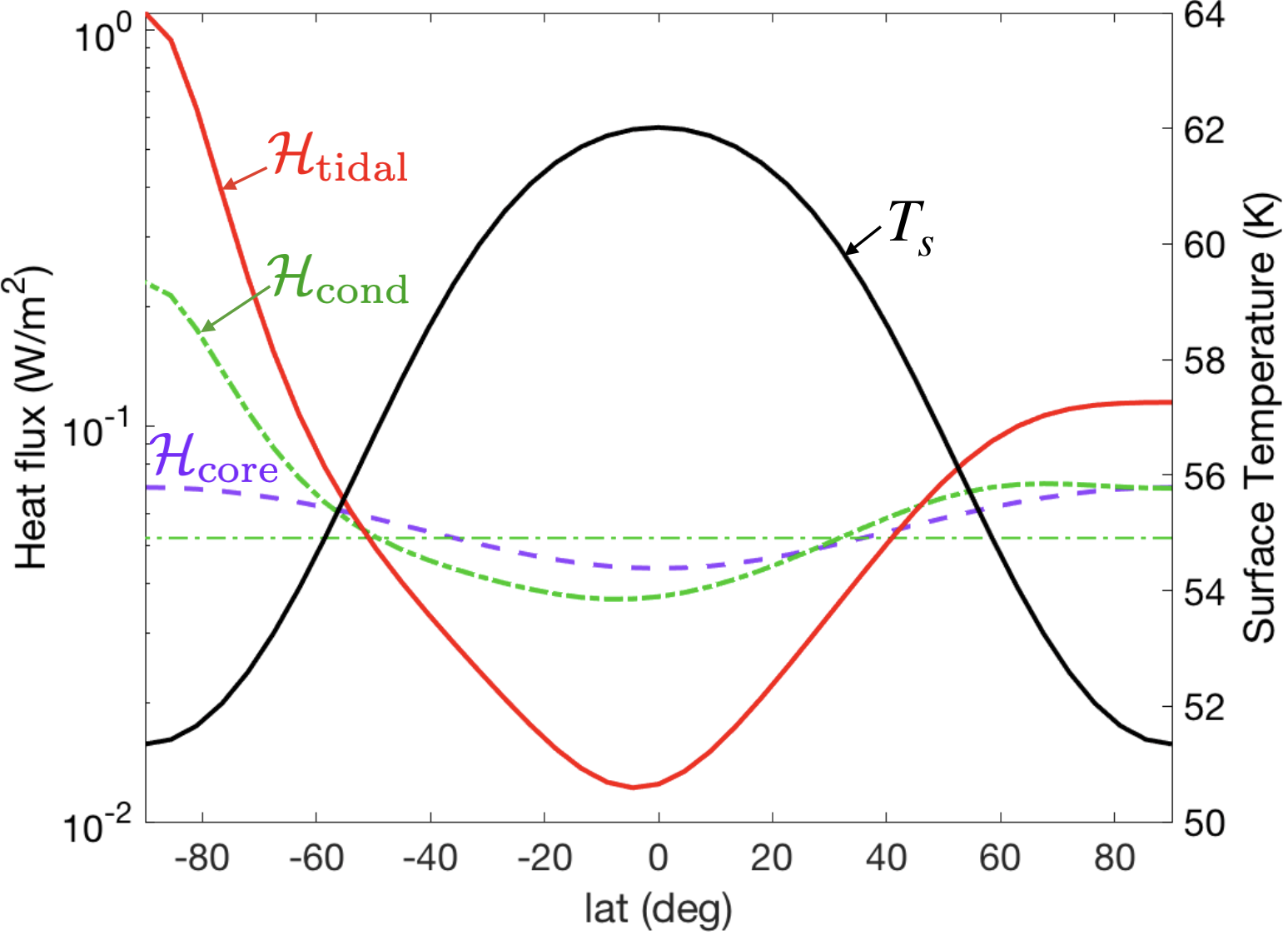
Figure S2: Meridional profiles of heat fluxes and surface temperature. Heat fluxes are plotted using colored curves, with a scale on the left. Conductive heat loss $\mathcal{H}_{\mathrm{cond}}$ (Eq. 8) is shown by a thick green dash-dotted line which, in the global average, is balanced by heat generation in the silicate core $\mathcal{H}_{\mathrm{core}}$ (purple dashed line, Eq. 9) and $\mathcal{H}_{\mathrm{ice}}$ (red solid line, Eq. 19). All heat fluxes are normalized to have the same global mean value of $\mathcal{H}_{\mathrm{cond}}$. The surface temperature $T_{s}$ (black solid line, axis on the right) is set to be in radiative equilibrium with the solar radiation and is warmer at the equator.

Tidal heating in the core

Conductive heat loss is primarily balanced by tidal dissipation in the ice shell $\mathcal{H}_{\mathrm{ice}}$ and the core $\mathcal{H}_{\mathrm{core}}$ (dissipation in the ocean plays a negligible role)  (?, ?, ?, ?). For each assumed heat partition between the shell and the core, we use the same meridional heating profiles for $\mathcal{H}_{\mathrm{core}}$ and $\mathcal{H}_{\mathrm{ice}}$ (see below). According to Beuthe 2019 (?) and Choblet et al. 2017 (?), the core dissipation $\mathcal{H}_{\mathrm{core}}$ peaks at the two poles. We obtain the meridional heat profile using Eq.60 in Beuthe 2019 (?) (Beuthe, personal communication),

$$\mathcal{H}_{\mathrm{core}}(\phi)=\bar{\mathcal{H}}_{\mathrm{core}}\cdot(1.08449+0.252257\cos(2\phi)+0.00599489\cos(4\phi)),$$ (9)

where $\phi$ denotes latitude and $\bar{\mathcal{H}}_{\mathrm{core}}$ is the global mean heat flux from the bottom. Since the global surface area shrinks going downward due to the spherical geometry, a factor of $\left.(a-H)^{2}\right/(a-H-D)^{2}$ ($H$ is ice thickness, $D$ is ocean depth) needs to be considered when computing $\bar{\mathcal{H}}_{\mathrm{core}}$. The expression within the bracket is normalized for the globe, adjusted to take account of the fact that our model only covers 84S-84N. Using the above formula, the bottom heat flux is twice as strong over the poles than equator, as can be seen in Fig.1d of the main text. We note that the heating profile here is highly idealized and does not have the localized heating stripes seen in Choblet et al. 2017  (?) which arise from the interaction between the porous core and the fluid in the gaps.

Ice-ocean fluxes

The interaction between ocean and ice is simulated using MITgcm’s “shelf-ice” package  (?, ?). We turn on the “boundary layer” option to avoid possible numerical instabilities induced by an ocean layer which is too thin. The code is modified to account for a gravitational acceleration that is very different from that on earth, the temperature dependence of heat conductivity, and the meridional variation of tidal heating generated inside the ice shell and the ice surface temperature. In the description that follows, we begin by introducing the shelf-ice parameterization in a fully coupled ocean-ice system and then make simplifications that fit our goal here.

Following Kang et al. 2020 (?), the freezing/melting rate of the ice shell is determined by a heat budget for a thin layer of ice at the base. The budget involves three terms: the heat transmitted upward by ocean $\mathcal{H}_{\mathrm{ocn}}$, the heat loss through the ice shell due to heat conduction $\mathcal{H}_{\mathrm{cond}}$ (Eq.8), and the tidal heating generated inside the ice shell $\mathcal{H}_{\mathrm{ice}}$ (Eq.19). As elucidated in Holland and Jenkins 1999  (?) and Losch 2008  (?), the continuity of heat flux and salt flux through the “boundary layer” gives,

$$\mathcal{H}_{\mathrm{ocn}}-\mathcal{H}_{\mathrm{cond}}+\mathcal{H}_{\mathrm{ice}}=-L_{f}q-C_{p}(T_{\mathrm{ocn-top}}-T_{b})q$$ (10)

$$\mathcal{F}_{\mathrm{ocn}}=-S_{b}q-(S_{\mathrm{ocn-top}}-S_{b})q,$$ (11)

where $T_{\mathrm{ocn-top}}$ and $S_{\mathrm{ocn-top}}$ denote the temperature and salinity in the top grid of the ocean, $S_{b}$ denotes the salinity in the “boundary layer”, and $q$ denotes the freezing rate in $kg/m^{2}/s$. $C_{p}=4000$ J/kg/K is the heat capacity of the ocean, $L_{f}=334000$ J/kg is the latent heat of fusion of ice.

$\mathcal{H}_{\mathrm{ocn}}$ and $\mathcal{F}_{\mathrm{ocn}}$ in Eq.10 can be written as

$$\mathcal{H}_{\mathrm{ocn}} = C_{p}(\rho_{0}\gamma_{T}-q)(T_{\mathrm{ocn-top}}-T_{b}),$$ (12)

$$\mathcal{F}_{\mathrm{ocn}} = (\rho_{0}\gamma_{S}-q)(S_{\mathrm{ocn-top}}-S_{b})$$ (13)

where $\gamma_{T}=\gamma_{S}=10^{-5}$ m/s are the exchange coefficients for temperature and salinity, and $T_{b}$ denotes the and temperature in the “boundary layer”. The terms associated with $q$ are the heat/salinity change induced by the deviation of $T_{\mathrm{ocn-top}},\ S_{\mathrm{ocn-top}}$ from that in the “boundary layer”, where melting and freezing occur. $T_{b}=T_{f}(S_{b},P)$, the freezing temperature at pressure $P$ and salinity $S_{b}$ (see Eq.7).

In a fully-coupled system, we would solve $S_{b}$ and $q$ from Eq. (10)-(13). When freezing occurs ($q>0$), the salinity flux $\rho_{w0}\gamma_{S}(S_{\mathrm{ocn-top}}-S_{b})$ is negative (downward). This leads to a positive tendency of salinity at the top of the model ocean, together with changes of temperature, thus:

$$\frac{dS_{\mathrm{ocn-top}}}{dt} = \frac{-\mathcal{F}_{\mathrm{ocn}}}{\rho_{w0}\delta z}=\frac{1}{\rho_{w0}\delta z}(\rho_{w0}\gamma_{S}-q)(S_{b}-S_{\mathrm{ocn-top}})=\frac{qS_{\mathrm{ocn-top}}}{\rho_{w0}\delta z},$$ (14)

$$\frac{dT_{\mathrm{ocn-top}}}{dt} = \frac{-\mathcal{H}_{\mathrm{ocn}}}{C_{p}\rho_{w0}\delta z}=\frac{1}{\rho_{w0}\delta z}(\rho_{w0}\gamma_{T}-q)(T_{b}-T_{\mathrm{ocn-top}})$$ (15)

$$= \frac{1}{C_{p}\rho_{w0}\delta z}\left[\mathcal{H}_{\mathrm{ice}}-\mathcal{H}_{\mathrm{cond}}+L_{f}q+C_{p}(T_{\mathrm{ocn-top}}-T_{b})q\right]$$

where $\delta z=2$ km is the thickness of the “boundary layer” at the ocean-ice interface.

If we allow the freezing/melting of ice and the ocean circulation to feedback onto one-another, the positive feedback between them renders it difficult to find consistent solutions. We therefore cut off this feedback loop by setting the freezing rate $q$ to that which is required to sustain the prescribed ice sheet geometry (details can be found in the next section, ice flow model), whilst allowing a heating term to balance the heat budget (Eq.10). The amplitude of this heat imbalance can then be used to discriminate between different steady state solutions (Eq. 1 in the main text). This also simplifies the calculation of the T/S tendencies of the upper-most ocean grid. The S tendency can be directly calculated from Eq. 14, and the T tendency approximated by:

$$\frac{dT_{\mathrm{ocn-top}}}{dt} = \frac{1}{\delta z}(\gamma_{T}-q)(T_{\mathrm{f,ocn-top}}-T_{\mathrm{ocn-top}}),$$ (16)

replacing the boundary layer freezing temperature $T_{b}=T_{f}(S_{b},P)$ in Eq. 15 with $T_{\mathrm{f,ocn-top}}=T_{f}(S_{\mathrm{ocn-top}},P)$, the freezing temperature determined by the upmost ocean grid salinity and pressure. The difference between the $S_{b}$ and $S_{\mathrm{ocn-top}}$ can be estimated by $\mathcal{F}_{\mathrm{ocn}}/(\rho_{0}\gamma_{S})=qS_{\mathrm{ocn-top}}/(\rho_{0}\gamma_{S})$, according to Eq.13 and Eq.14, given that $|q|\lesssim 10^{-7}$ kg/$m^{2}$/s is orders of magnitude smaller than $\rho_{0}\gamma_{S}=0.01$ kg/m²/s. Even in the saltiest scenario we consider here, $|S_{b}-S_{\mathrm{ocn-top}}|$ does not exceed $0.0004$ psu, and the associated freezing point change is lower than $10^{-5}$K. Readers interested in the formulation of a freely evolving ice-water system are referred to the method section of Kang et al. 2021 (?) and Losch 2008 (?).

In addition to the above conditions on temperature and salinity, the tangential velocity is relaxed back to zero at a rate of $\gamma_{M}=10^{-3}$m/s at the upper and lower boundaries.

Ice flow model

We prescribe $q$ using the divergence of the ice flow, assuming the ice sheet geometry is in equilibrium. We use an upside-down land ice sheet model following Ashkenazy et al. 2018  (?). The ice flows down its thickness gradient, driven by the pressure gradient induced by the spatial variation of the ice top surface, somewhat like a second order diffusive process. At the top, the speed of the ice flow is negligible because the upper part of the shell is so cold and hence rigid; at the bottom, the vertical shear of the ice flow speed vanishes, as required by the assumption of zero tangential stress there. This is the opposite to that assumed in the land ice sheet model. In rough outline, we calculate the ice flow using the expression below obtained through repeated vertical integration of the force balance equation (the primary balance is between the vertical flow shear and the pressure gradient force), using the aforementioned boundary conditions to arrive at the following formula for ice transport $\mathcal{Q}$,

$$\mathcal{Q}(\phi) = \mathcal{Q}_{0}H^{3}(\partial_{\phi}H/a)$$ (17)

$$\mathcal{Q}_{0} = \frac{2(\rho_{0}-\rho_{i})g}{\eta_{\mathrm{melt}}(\rho_{0}/\rho_{i})\log^{3}\left(T_{f}/T_{s}\right)}\int_{T_{s}}^{T_{f}}\int_{T_{s}}^{T(z)}\exp\left[-\frac{E_{a}}{R_{g}T_{f}}\left(\frac{T_{f}}{T^{\prime}}-1\right)\right]\log(T^{\prime})~{}\frac{dT^{\prime}}{T^{\prime}}~{}\frac{dT}{T}.$$

Here, $\phi$ denotes latitude, $a=252$ km and $g=0.113$ m/s² are the radius and surface gravity of Enceladus, $T_{s}$ and $T_{f}$ are the temperature at the ice surface and the water-ice interface (equal to local freezing point, Eq. 7), and $\rho_{i}=917$ kg/m³ and $\rho_{0}$ are the ice density and the reference water density (Eq. 5). $E_{a}=59.4$ kJ/mol is the activation energy for diffusion creep, $R_{g}=8.31$ J/K/mol is the gas constant and $\eta_{\mathrm{melt}}$ is the ice viscosity at the freezing point. The latter has considerable uncertainty ($10^{13}$-$10^{16}$ Pa$\cdot$s)  (?) but we choose to set $\eta_{\mathrm{melt}}=10^{14}$ Pa$\cdot$s.

In steady state, the freezing rate $q$ must equal the divergence of the ice transport thus:

$$q=-\frac{1}{a\cos\phi}\frac{\partial}{\partial\phi}(Q\cos\phi).$$ (18)

As shown by the dashed curve in Fig.1b of the main text, ice melts in high latitudes and forms in low latitudes at a rate of a few kilometers every million years. A more detailed description of the ice flow model can be found in Kang and Flierl 2020 (?) and Ashkenazy et al. 2018  (?). Freezing and melting leads to changes in local salinity and thereby a buoyancy flux. At $S_{0}=30$ psu, the salinity-associated buoyancy flux is approximately $gq\beta_{S}S_{0}\approx 10^{-13}$ m²/s³, which is 3-6 orders of magnitude smaller than the buoyancy flux used by Lobo et al. 2021 (?).

1.5 Model of tidal dissipation in the ice shell

Enceladus’s ice shell is periodically deformed by tidal forcing and the resulting strains in the ice sheet produce heat. We follow Beuthe 2019 (?) to calculate the implied dissipation rate. Instead of repeating the whole derivation here, we only briefly summarize the procedure and present the final result. Unless otherwise stated, parameters are the same as assumed in Kang & Flierl 2020 (?).

Tidal dissipation consists of three components  (?): a membrane mode $\mathcal{H}_{\mathrm{ice}}^{\mathrm{mem}}$ due to the extension/compression and tangential shearing of the ice membrane, a mixed mode $\mathcal{H}_{\mathrm{ice}}^{mix}$ due to vertical shifting, and a bending mode $\mathcal{H}_{\mathrm{ice}}^{bend}$ induced by the vertical variation of compression/stretching. Following Beuthe 2019 (?), we first assume the ice sheet to be completely flat. By solving the force balance equation, we obtain the auxiliary stress function $F$, which represents the horizontal displacements, and the vertical displacement $w$. The dissipation rate $\mathcal{H}_{\mathrm{ice}}^{\mathrm{flat,x}}$ (where $x=\{\mathrm{mem},\mathrm{mix},\mathrm{bend}\}$ ) can then be written as a quadratic form of $F$ and $w$. In the calculation, the ice properties are derived assuming a globally-uniform surface temperature of 60K and a melting viscosity of $5\times 10^{13}$ Pa$\cdot$s.

Ice thickness variations are accounted for by multiplying the membrane mode dissipation $\mathcal{H}_{\mathrm{ice}}^{\mathrm{flat,mem}}$, by a factor that depends on ice thickness. This makes sense because this is the only mode which is amplified in thin ice regions (see Beuthe 2019 (?)). This results in the expression:

$$\mathcal{H}_{\mathrm{ice}}=(H/H_{0})^{p_{\alpha}}\mathcal{H}_{\mathrm{ice}}^{\mathrm{flat,mem}}+\mathcal{H}_{\mathrm{ice}}^{\mathrm{flat,mix}}+\mathcal{H}_{\mathrm{ice}}^{\mathrm{flat,bend}},$$ (19)

where $H$ is the prescribed thickness of the ice shell as a function of latitude and $H_{0}$ is the global mean of $H$. Since thin ice regions deform more easily and produce more heat, $p_{\alpha}$ is negative. Because more heat is produced in the ice shell, the overall ice temperature rises, which, in turn, further increases the mobility of the ice and leads to more heat production (the rheology feedback).

Using reasonable parameters for Enceladus, $\mathcal{H}_{\mathrm{ice}}$ turns out to be at least an order of magnitude smaller than the heat loss rate $\mathcal{H}_{\mathrm{cond}}$. This is a universal flaw of present tidal dissipation models, and could be due to use of an over-simplified Maxwell rheology  (?, ?). We therefore scale up $\mathcal{H}_{\mathrm{ice}}$ by a constant factor to obtain the desired magnitude. The tidal heating profile corresponding to $p_{\alpha}=-1.5$ is the red solid curve plotted in Fig. S2. In Fig. 4(b,e) of the main text, we show the tidal heating profile for $p_{\alpha}=-1$ and $p_{\alpha}=-2$.

Symbol	Name	Definition/Value
Enceladus parameters
$a$	radius	252 km
$\delta$	obliquity	27∘
$H$	global mean ice thickness	20.8 km: ref  (?)
$D$	global mean ocean depth	39.2 km: ref  (?)
$\Omega$	rotation rate	5.307$\times$10-5 s-1
$g_{0}$	surface gravity	0.113 m/s2
$\bar{T_{s}}$	mean surface temperature	59K
Europa parameters
$a$	radius	1561 km
$\delta$	obliquity	3.1∘
$H$	global mean ice thickness	15 km: ref  (?)
$D$	global mean ocean depth	85 km: ref  (?)
$\Omega$	rotation rate	2.05$\times$10-5 s-1
$g_{0}$	surface gravity	1.315 m/s2
$\bar{T_{s}}$	mean surface temperature	110K
Physical constants
$L_{f}$	fusion energy of ice	334000 J/kg
$C_{p}$	heat capacity of water	4000 J/kg/K
$T_{f}(S,P)$	freezing point	Eq.7
$\rho_{i}$	density of ice	917 kg/m3
$\rho_{w}$	density of the ocean	Eq.5
$\alpha,\beta$	thermal expansion & saline contraction coeff.	using Gibbs Seawater Toolbox: ref  (?)
$\kappa_{0}$	conductivity coeff. of ice	651 W/m: ref  (?)
$p_{\alpha}$	ice dissipation amplification factor	-2 $\sim$ -1
$\eta_{m}$	ice viscosity at freezing point	1014 Ps$\cdot$s
Default parameters in the ocean model
$\nu_{h},\ \nu_{v}$	horizontal/vertical viscosity	50 m2/s
$\tilde{\nu}_{h},\ \tilde{\nu}_{v}$	bi-harmonic hyperviscosity	3$\times$109 m4/s
$\kappa_{h},\ \kappa_{v}$	horizontal/vertical diffusivity	0.005 m2/s
$\kappa_{\mathrm{GM}}$	Gent-McWilliams diffusivity	0.1 m2/s
$(\gamma_{T},\ \gamma_{S},\ \gamma_{M})$	water-ice exchange coeff. for T, S & momentum	(10-5, 10-5, 10-3) m/s
$g$	gravity in the ocean	Eq.1
$P_{0}$	reference pressure	$\rho_{i}g_{0}H=2.16\times 10^{6}$ Pa
$T_{0}$	reference temperature	$T_{f}(S_{0},P_{0})$
$\rho_{w0}$	reference density of ocean	Eq.6
$\mathcal{H}_{\mathrm{cond}}$	conductive heat loss through ice	Eq.8, Fig.S2
$\mathcal{H}_{\mathrm{ice}}$	tidal heating produced in the ice	Eq.19, Fig.S2
$\mathcal{H}_{\mathrm{core}}$	bottom heat flux powered by the core	Eq.9, Fig.S2
$A$	surface albedo	0.81
$T_{s}$	surface temperature profile	Fig.S2

Table 1: Model parameters used in our study.

Control exp	sensitivity-1	sensitivity-2	sensitivity-3	Conceptual model
1.5	1.1	1.1	0.6	2.9
2.0	1.2	0.3	0.2	2.2
0.95	0.5	0.3	0.3	0.44
1.2	0.7	0.4	0.4	0.8
1.5	0.92	0.5	0.4	1.3
1.8	1.0	0.5	0.4	1.9
2.1	1.2	0.6	0.5	2.5
2.3	1.3	0.6	0.6	3.2
2.4	1.5	0.7	0.6	3.8

Table 2: The maximum northern-hemispheric streamfunctions (in unit of $10^{8}$ kg/s) in numerical models and the conceptual model. The control experiment parameters can be found in Tab. 1. Sensitivity test 1 is the same as control except that $\kappa_{\mathrm{GM}}=0$ m²/s. Sensitivity test 2 uses $\kappa_{\mathrm{GM}},\kappa_{v},\kappa_{h}=0,10^{-3},10^{-3}$ m²/s. Sensitivity test 3 uses $\kappa_{\mathrm{GM}},\kappa_{v},\kappa_{h}=0,10^{-3},10^{-5}$ m²/s. When changing diffusivity, the circulation depth also changes, so the absolute values of streamfunction are not directly comparable from one group of experiments to another. However, the general trends are very similar – as salinity increases, the streamfunction first decreases then increases.

2 Exploring the sensitivity of ocean model solutions to parameters

2.1 Sensitivity to heat partition between the core and the shell

To examine the sensitivity of ocean circulation to core-shell heat partition, we repeat the same set of simulations with first 20% and then 100% heat produced in the core. The equilibrium ocean solutions are presented in Fig.S3 and Fig.S4 for the two heat partitions. Compared to our default calculation, the shell-heating scenario shown in Fig.3 of the main text, there is no qualitative change. This is to be expected because the dominant forcing of the flow is the salinity and heat exchange between ice and ocean: the vertical temperature gradient induced by bottom heating is much smaller than the temperature gradient at the water-ice interface induced by the pressure dependence of the freezing point of water. Bottom warming induces stronger stratification if the ocean is fresher than 22 psu (when $\alpha<0$), and vice versa. As can be seen by comparing Fig.S3 and Fig.S4 with Fig.3, the strengthening/weakening of the stratification suppresses/enhances the vertical extent over which the overturning circulation reaches into the deep ocean. The change is most pronounced at low salinity (4 psu), because the negative thermal expansion coefficient in a fresh ocean suppresses the parameterized convection, resulting in bottom water warming up. However, even with a mean salinity of 4 psu, the response of the dynamics to these stratification changes is rather small (compare the left columns of Fig.3 and Fig.S4 here). Note also that all experiments are run out to full equilibrium and so the bottom heat flux is transmitted upward to the water-ice interface without loss in an integral sense, but with ocean currents shaping regional contributions.

Figure S3: As in Fig. 3 of the main text but with 20% heat assumed to be produced in the silicate core and 80% in the ice shell. Results are presented for three different salinities: 4 psu, 10 psu and 40 psu. Default mixing parameters are used.

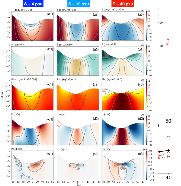
Figure S4: As in Fig.S3 but with 100% heating in the core and none in the shell. Default mixing parameters are used.

2.2 Sensitivity to diffusivity and viscosity

To examine the sensitivity to diffusivity, we carried out three additional sets of experiments for the shell-heating scenario using different GM and diapycnal diffusivities: one with $\kappa_{\mathrm{GM}}=0$ m²/s, $\kappa_{v}=\kappa_{h}=5\times 10^{-3}$ m²/s, one with $\kappa_{\mathrm{GM}}=0$ m²/s, $\kappa_{v}=\kappa_{h}=10^{-3}$ m²/s, and the third with $\kappa_{\mathrm{GM}}=0$ m²/s, $\kappa_{v}=10^{-5}$ m²/s, $\kappa_{h}=10^{-3}$ m²/s. The corresponding solutions for $S_{0}=4,\ 10$ and $40$ psu are shown in Fig. S5, Fig. S6 and Fig. S7, respectively. The mismatch index that measures the discrepancy between the inferred and predicted ice tidal dissipation (Eq. 2 in the main text) are plotted on Fig. 4c in the main text using triangular markers.

On changing GM and diapycnal diffusivities, the dependence of the meridional heat transport and hence the inferred tidal dissipation on salinity remains qualitatively similar to the control experiments: compare the bottom panels of Fig. S5, Fig. S6 and Fig. S7 with Fig. 4b in the main text. The mismatch between the inferred tidal dissipation $\hat{\mathcal{H}}_{\mathrm{ice}}$ and the modeled dissipation $\mathcal{H}_{\mathrm{ice}}$ is smallest when the reference salinity is in the range 10-20 psu regardless of the spread of diffusivities being used. The ocean solutions also remain qualitatively similar to the control experiments shown in Fig. 3 in the main text. Low salinity cases have sinking over the poles, driven in the main by the density gradient associated with temperature anomalies (see left panels of Fig. S5, Fig. S6 and Fig. S7). The opposite is true for the high salinity cases (see the right panels). At intermediate salinities ($\sim$10 psu), the density gradient and overturning circulation are weak (see the middle panels), just as in the control solution (Fig. 3 in the main text). This weak circulation, in turn, leads to a weaker heat convergence toward the equator compared to the end-member cases (see Fig. S5f, Fig. S6f and Fig. S7f and Fig. 4b in the main text), and the resulting $\hat{\mathcal{H}}_{\mathrm{ice}}$ is more consistent with $\mathcal{H}_{\mathrm{ice}}$ (black dashed curves). This general trend is found in all diffusivity scenarios (Fig. 4c in the main text), suggesting that our main conclusions are indeed robust.

There are quantitative changes to our solutions, however. When GM is turned off, the overall stratification becomes weaker due to the lack of parameterized slantwise convection, the isopycnal slope becomes steeper (row-c of Fig. S5 and Fig. 3 in the main text), the salinity contrast is slightly reduced (row-b of Fig. S5 and Fig. 3 in the main text) and the circulation weakens. Furthermore, reducing the explicit diffusivity suppresses mixing and increases salinity/temperature variations over the globe (Fig. S6 and Fig. S7). That leads to stronger stratification, shallower circulation and weaker meridional heat transport, as can be seen by comparing Fig. S6 and Fig. S7 against Fig. S5. These changes are particularly significant in the 40 psu case perhaps because the ocean circulation cannot be efficiently energized when the buoyancy source is located higher in the water column than the buoyancy sink  (?).

We also carried out two sets of experiments to test the sensitivity to lower viscosity. The solutions with default diffusivities but 5 times lower viscosities ($\nu_{v}=\nu_{h}=10$ m²/s instead of $50$ m²/s) are shown in Fig. S8. To reduce grid-scale noise caused by the low viscosity, the streamfunctions (row-e) and the heat transport curve (row-f) were smoothed. While the temperature, salinity, zonal flow fields remains almost identical to the control experiments (Fig. 3 in the main text), the overturning circulation follows the Taylor columns more closely. Without viscosity, the angular momentum of water conserves before it encounters the rough boundary at the top or bottom, and as a result, flow must follow the direction of rotating axis to avoid drastic change in zonal momentum, which would require strong density variation according to the thermal wind balance. The meridional heat transport decreases by only by a small portion, leading to a slightly lower mismatch index, as can be seen from Fig. 4 in the main text (dots indicate the default setup and left triangle the case with low viscosity).

When the viscosities are further reduced to $\nu_{v}=\nu_{h}=2$ m²/s, 25 times lower than the default viscosities, the vertical flow speed becomes pixelated (not shown). Although we usually avoid noises like this by increasing damping, they sometimes show up in proper solutions for terrestrial ocean when the resolution is coarse, leaving the solution’s relevance somewhat uncertain. In row-e of Fig. S9 and Fig. S10, we present the smoothed streamfunction for the 4 psu, 10 psu and 40 psu scenarios. It is noticeable that the shallow cells along the ice shell disappear, and a deeper circulation that is overridden before shows up. This deep circulation closely follows the tangent cylinder and connects the ice shell all the way to the seafloor.

To understand this change, we need to consider the momentum budget. When water moves toward (away from) the rotating axis under the influence of pressure gradient, by conserving angular momentum, the flow will tend to accelerate eastward (westward). This tendency has to be removed by either friction or viscosity, otherwise the resultant zonal jet will form the so-called geostrophic balance with the pressure gradient force, the driving force of the meridional circulation. The roughness of the water-ice interface and the seafloor allows water to move along these two boundaries meridionally. In the interior, without boundary friction, flow tends to be aligned with the direction of the rotating axis to avoid zonal acceleration, unless viscosity can transport the gained zonal momentum toward a rough boundary nearby, so that momentum can be dissipated. In the viscous layer, the dominant momentum balance should be

$$fV\sim\nu_{v}\partial_{z}\partial_{z}U\sim\nu_{v}\frac{\Delta U}{\delta^{2}},$$ (20)

where $V$ and $U$ denote flow speeds in north/south direction and east/west direction, respectively, $\Delta U$ denotes the zonal speed difference between upper branch and lower branch of the shallow cell, and $\delta$ denotes the depth of the return flow. Assuming that $\Delta U$ is 1-2 order of magnitude greater than $V$, the depth of return flow should be around $\delta=\sqrt{50\nu_{v}/f}\sim 5$ km ($\nu_{v}=50$ m²/s, $\Delta U/V=50$ is used here), two times the model’s vertical resolution (2 km). That is why the shallow cell is resolved in the default setup. As viscosity decreases, the lower branch needs to move closer to the ice shell to feel the viscous force. With $\nu_{v}=1$ m²/s, $\delta$ decreases to $0.7$ km, and therefore, the $2$ km vertical resolution can no longer resolve the cell.

How deep the shallow circulation can extend in reality depends on the vertical viscosity. On Enceladus, the ice shell wobbles back and forth by roughly 100 m due to its eccentricity on the timescale of rotation period  (?, ?). This by itself will leads to a viscosity around $1$ m²/s. Besides, shear instability may arise when the flow shear is greater than the stratification, $U_{z}\sim\Delta U/\delta>2N$ ($N$ is the Brunt-Vasala frequency). In a weakly stratified environment like Enceladus, the above instability condition should be easy to satisfy and the resultant eddies may further enhance the viscosity.

Although the circulation looks very different in experiments with and without the shallow cells, the heat transport doesn’t seem to vary by a lot. This can be seen by comparing Fig. S9f and Fig. S10f with Fig. 3f in the main text and Fig. S6f here, respectively. Since the salinity flux from the ice shell is fixed in all experiments, when ocean circulates slowly, salinity anomaly will accumulate. This will drive stronger circulation in a salty ocean, keeping the heat transport roughly the same.

We also carried out sensitivity tests for the core-heating scenario as shown in Fig. S11 with $\kappa_{\mathrm{GM}}=0$ and in Fig. S12 and low horizontal and vertical diffusivities ($\kappa_{h}=10^{-3}$ m²/s, $\kappa_{v}=10^{-5}$ m²/s). Again, the solutions are very similar to those with a GM parameterization and higher diffusivities (Fig. S4), except for weaker stratification, weaker isopycnal slope, salinity contrast and circulation, relative to the shell-heating scenario with default parameters.

Figure S5: The 100% shell-heating solution with default parameters except $\kappa_{\mathrm{GM}}=0$ m²/s. Row (a-e) are the same figure as in Fig.3 of the main text. Row (f) is similar to Fig. 4(b,e) of the main text and shows the inferred tidal dissipation $\hat{\mathcal{H}}_{\mathrm{ice}}$ (red solid line, calculated using Eq. 1 in the main text), compared with the dissipation rate predicted by our tidal dissipation model (black dashed lines, Eq.19).

Figure S6: The sensitivity of the 100% shell-heating solution to lower explicit diffusivity ($\kappa_{\mathrm{GM}}=0$ m²/s, $\kappa_{v}=\kappa_{h}=10^{-3}$ m²/s), set out as in Fig. S5.

Figure S7: The sensitivity of the 100% shell-heating solution to even lower explicit diffusivity ($\kappa_{\mathrm{GM}}=0$ m²/s, $\kappa_{v}=10^{-5}$ m²/s, $\kappa_{h}=10^{-3}$ m²/s), set out as in Fig. S5. The interval between salinity and density contours are 20 times larger than in other plots.

Figure S8: The sensitivity of the shell-heating scenario solution to lower viscosity ($\nu_{v}=\nu_{h}=10$ m²/s instead of $50$ m²/s). Row (a-e) are the same figure as Fig.3 in the main text, showing the ocean circulation and thermodynamic state. Row (f) is similar to Fig. 4(b,e) in the main text, showing the inferred tidal dissipation $\hat{\mathcal{H}}_{\mathrm{ice}}$ (red solid line, calculated using Eq. 1 in the main text), in comparison with the dissipation rate predicted by tidal dissipation model (black dashed lines, Eq.19). To remove the grid-size noise from the heat transport profile, we apply a 9-point smoothing.

Figure S9: The sensitivity of the shell-heating scenario solution to even lower viscosity ($\nu_{v}=\nu_{h}=1$ m²/s instead of $50$ m²/s). To remove the grid-size noise from the heat transport and streamfunction profiles, we apply a 9-point smoothing.

Figure S10: Same as Fig.S9 except lower diffusivity is used ($\kappa_{v}=\kappa_{h}=10^{-3}$ m²/s). To remove the grid-size noise from the heat transport and streamfunction profiles, we apply a 9-point smoothing.

Figure S11: The sensitivity of the 100% core-heating solution to zero GM diffusivity ($\kappa_{\mathrm{GM}}=0$ m²/s, $\kappa_{v}=\kappa_{h}=5\times 10^{-3}$ m²/s), set out as in Fig. S5.

Figure S12: The sensitivity of the 100% core-heating solution to low diffusivities ($\kappa_{\mathrm{GM}}=0$ m²/s, $\kappa_{v}=10^{-5}$ m²/s, $\kappa_{h}=10^{-3}$ m²/s), set out as in Fig. S5. Note that the interval between two contour lines for salinity and density are 5 times greater than Fig. S11 ($10^{-2}$ psu, $10^{-2}$ kg/m³).

2.3 Sensitivity to assumed ice viscosity

The viscosity of the ice shell controls ice speeds (Eq. 17), and thereby the freezing/melting rate needed to maintain the observed ice geometry. However, due to our limited understanding of ice rheology, the uncertainties associated with the melting point ice viscosity $\eta_{m}$ remain. To examine sensitivity we carried out an experiment with $\eta_{m}$ set to $2\times 10^{13}$ Pa$\cdot$s, 5 times lower than the default value. Solutions for $S_{0}=4,\ 10,\ 40$ psu are presented in Fig. S13. Decreasing the ice viscosity leads to a stronger salinity flux between the ocean and ice (Eq. 14) and stronger salinity variations. This can be clearly seen by comparing Fig. S13b with Fig. 3b of the main text. Since the overall salinity gradient increases, the density gradient also increases (Fig. S13c), and this in turn drives stronger circulation (Fig. S13e). In addition to these change, increasing ice mobility lowers the transitional salinity as shown by plus sign symbols in Fig. 4c of the main text. That is because a more negative thermal expansion coefficient is required to cancel the salinity-induced density anomaly and achieve a minimum density gradient, indeed just as suggested by our conceptual model. The opposite is true with increased ice viscosity. Because the salinity flux between the ocean and ice decreases, the overall salinity gradient decreases, and that make cancellation between the temperature- and salinity-driven circulation occur at higher salinity (15 psu instead of 10 psu, see minus sign symbols in Fig. 4c of the main text).

Figure S13: The sensitivity of the 100% shell-heating scenario solution to lower ice viscosity ($\eta_{m}=2\times 10^{13}$ Pa$\cdot$s instead of $10^{14}$ Pa$\cdot$s), set out as in Fig. S5. Default ocean mixing parameters are used.

Figure S14: The sensitivity of the 100% shell-heating scenario solution to higher ice viscosity ($\eta_{m}=5\times 10^{14}$ Pa$\cdot$s instead of $10^{14}$ Pa$\cdot$s), set out as in Fig. S5. Default ocean mixing parameters are used.

2.4 Sensitivity to higher resolution and 3D dynamics

We also carried out sensitivity tests at higher spatial resolution and assuming 3D rather than 2D dynamics. Doubling the resolution does not change the solution in any significant way (compare Fig. S15 and Fig.3 in the main text), indicating that our default solutions are robust to increasing resolution. Adding a third dimension allows zonal wave structures to form, which transport additional heat especially when the salinity is low (see Fig. S16-f1). However, the best-match heat budget again occurs at intermediate salinities (see Fig. S16 row-f). The detailed wave dynamics is not the focus of the present study and is left for further work.

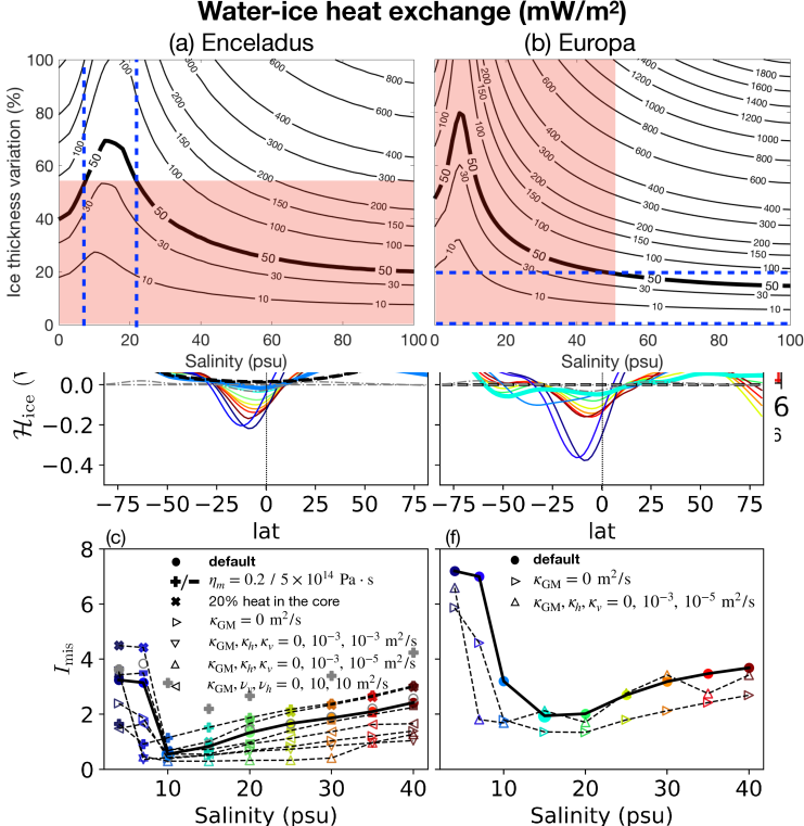
Figure S15: The sensitivity of the 100% shell-heating scenario solution to higher resolution (1 degree instead of 2 degree), set out as in Fig. S5. Default parameters are used.

Figure S16: The sensitivity of the 100% shell-heating scenario solution to 3D configuration. Physical parameters are the same as Fig. S13, except that cube sphere (cs32) grid is used. The dashed curves show the ice dissipation predicted by tidal model assuming $p_{\alpha}=-1.5$ and $p_{\alpha}=-3$, respectively.

2.5 Experiments under hemispherically-symmetric forcing

In further tests we carried out experiments under hemispherically symmetric ice geometry and forcing allowing for comparison with theoretical model results reported by Lobo et al. 2021  (?). The symmetric ice geometry used here is constructed by averaging the default ice thickness profile shown in Fig. 1b between the two hemispheres. The freezing/melting rate forcing is calculated as before (Eq 17) and the freezing point temperature imposed as a function of pressure. Symmetric ocean solutions are shown on the left column of Fig. S17 together with inferred tidal dissipation rates $\hat{\mathcal{H}}_{\mathrm{ice}}$ with default diffusivities ($\kappa_{\mathrm{GM}}=0.1$ m²/s, $\kappa_{v}=\kappa_{h}=5\times 10^{-3}$ m²/s). Tracer distributions, circulation and zonal flow are all symmetric about the equator due to the symmetry in the forcing. The mean salinity is set to 30 psu to avoid anomalous expansion effects, and we assume all heat is produced in the ice shell. This broadly mimics the setup used by Lobo et al. 2021  (?).

As found by Lobo et al. 2021  (?), the near-surface isopycnals tilt downward in polar regions (Fig. S17-c1), driving meridional circulation confined to the near-surface layer (Fig. S17-e1). As in Lobo et al. 2021  (?), we explored the sensitivity of our solution to mixing coefficients. The middle and right columns of Fig. S17 present solutions obtained using two different diapycnal diffusivities with $\kappa_{\mathrm{GM}}=0$ m²/s). By turning off the GM parameterization we again observe the circulation and stratification becoming weaker (Fig. S17-e2 and Fig. S17-c2). Furthermore, when lower diapycnal diffusivity is used, the stratification strengthens (Fig. S17-c3) and the circulation becomes weaker and shallower (Fig. S17-e3).

Finally, it should be noted that the GM diffusivity used here, $\kappa_{\mathrm{GM}}=0.1$ m²/s, is estimated based on our arguments that lateral mixing scales are a few kilometers and the eddy flow speed a few millimeters per second (see Eq 4). This is several orders of magnitude smaller than the range explored by Lobo et al. 2021  (?), which was presumably motivated by those typical of Earth’s ocean. Furthermore, in order to sustain the observed ice geometry  (?), we argue that the freezing/melting rate is a few kilometers per million years. This can be converted to a buoyancy flux by multiplying the haline contract coefficient $\beta_{S}$, ocean mean salinity $S_{0}$ and gravity $g$. Substituting parameters appropriate to Enceladus yields a buoyancy flux of the order of $10^{-13}$ m²/s³. This is a full 3-6 orders of magnitude smaller than that used in Lobo et al. 2021  (?). Due to these differences, we prefer not to make quantitative comparison with Lobo et al. 2021  (?).

Figure S17: Solutions under hemispherically-symmetric forcing with the mean salinity set to 30 psu. The left column shows results for default diffusivities ($\kappa_{\mathrm{GM}}=0.1$ m²/s, $\kappa_{v}=\kappa_{h}=5\times 10^{-3}$ m²/s), the middle column sets the GM diffusivity to zero ($\kappa_{\mathrm{GM}}=0$ m²/s, $\kappa_{v}=\kappa_{h}=5\times 10^{-3}$ m²/s), and the right column reduces ocean mixing coefficients ($\kappa_{\mathrm{GM}}=0$ m²/s, $\kappa_{v}=\kappa_{h}=10^{-3}$ m²/s).

References

- 1. MITgcm-group, MITgcm User Manual, Online documentation, MIT/EAPS, Cambridge, MA 02139, USA (2010). http://mitgcm.org/public/r2_manual/latest/online_documents/manual.html.
- 2. J. Marshall, A. Adcroft, C. Hill, L. Perelman, C. Heisey, J. Geophys. Res. 102, 5,753 (1997).
- 3. M. Losch, J. Geophys. Res. 113, 10.1029/2007JC004368 (2008).
- 4. D. J. Hemingway, T. Mittal, Icarus 332, 111 (2019).
- 5. J. Rekier, A. Trinh, S. Triana, V. Dehant, Journal of Geophysical Research: Planets 124, 2198 (2019).
- 6. C. Wunsch, R. Ferrari, Ann. Rev. Fluid Mech. 36, 281 (2004).
- 7. B. A. Klinger, J. Marshall, U. Send, Journal of Geophysical Research: Oceans 101, 18175 (1996).
- 8. W. Kang, et al., arXiv preprint arXiv:2008.03764 (2020).
- 9. H. Jones, J. Marshall, J. Phys. Oceanogr. 23, 1009 (1993).
- 10. M. H. Redi, J. Phys. Oceanogr. 12, 1154 (1982).
- 11. P. R. Gent, J. C. Mcwilliams, Journal of Physical Oceanography 20, 150 (1990).
- 12. M. Visbeck, J. Marshall, T. Haine, M. Spall, J. Phys. Oceanogr. 27, 381 (1997).
- 13. A. H. Lobo, A. F. Thompson, S. D. Vance, S. Tharimena, Nature Geoscience pp. 1–5 (2021).
- 14. T. J. McDougall, P. M. Barker, SCOR/IAPSO WG 127, 1 (2011).
- 15. T. J. McDougall, D. R. Jackett, D. G. Wright, R. Feistel, Journal of Atmospheric and Oceanic Technology 20, 730 (2003).
- 16. R. Tajeddine, et al., Icarus 295, 46 (2017).
- 17. Chen, E M A, Nimmo, F, Icarus 214, 779 (2011).
- 18. M. Beuthe, Icarus 280, 278 (2016).
- 19. H. C. F. C. Hay, I. Matsuyama, Icarus 319, 68 (2019).
- 20. M. Beuthe, Icarus 332, 66 (2019).
- 21. G. Choblet, et al., Nature Astronomy 1, 841 (2017).
- 22. D. M. Holland, A. Jenkins, J. Phys. Oceanogr. 29, 1787 (1999).
- 23. M. Beuthe, Icarus 302, 145 (2018).
- 24. Y. Ashkenazy, R. Sayag, E. Tziperman, Nature Astronomy 2, 43 (2018).
- 25. G. Tobie, G. Choblet, C. Sotin, J. Geophys. Res - Atmospheres 108, 219 (2003).
- 26. W. Kang, G. Flierl, PNAS 117, 14764 (2020).
- 27. C. McCarthy, R. F. Cooper, Earth and Planetary Science Letters 443, 185 (2016).
- 28. J. P. Renaud, W. G. Henning, Astrophysical Journal 857, 98 (2018).
- 29. K. Hand, C. Chyba, Icarus 189, 424 (2007).
- 30. V. Petrenko, R. Whitworth, Physics of Ice (OUP Oxford, 1999).
- 31. Y. Zeng, M. F. Jansen, arXiv preprint arXiv:2101.10530 (2021).
- 32. D. Lemasquerier, et al., Journal of Geophysical Research: Planets 122, 1926 (2017).