Fast quantum state reconstruction
via accelerated non-convex programming

Abstract

We propose a new quantum state reconstruction method that combines ideas from compressed sensing, non-convex optimization, and acceleration methods. The algorithm, called Momentum-Inspired Factored Gradient Descent (MiFGD), extends the applicability of quantum tomography for larger systems. Despite being a non-convex method, MiFGD converges provably close to the true density matrix at an accelerated linear rate, in the absence of experimental and statistical noise, and under common assumptions. With this manuscript, we present the method, prove its convergence property and provide Frobenius norm bound guarantees with respect to the true density matrix. From a practical point of view, we benchmark the algorithm performance with respect to other existing methods, in both synthetic and real experiments performed on an IBM’s quantum processing unit. We find that the proposed algorithm performs orders of magnitude faster than state of the art approaches, with the same or better accuracy. In both synthetic and real experiments, we observed accurate and robust reconstruction, despite experimental and statistical noise in the tomographic data. Finally, we provide a ready-to-use code for state tomography of multi-qubit systems.

Introduction

Quantum tomography is one of the main procedures to identify the nature of imperfections and deviations in quantum processing unit (QPU) implementation [9, 27]. Generally, quantum tomography is composed of two main parts: $i)$ measuring the quantum system, and $ii)$ analyzing the measurement data to obtain an estimation of the density matrix (in the case of state tomography [9]), or of the quantum process (in the case of process tomography [66]). In this manuscript, we focus on the case of state tomography.

As the number of free parameters that define quantum states and processes scale exponentially with the number of subsystems, generally quantum tomography is a non-scalable protocol [38]. In particular, quantum state tomography (QST) suffers from two bottlenecks related to its two main parts. The first concerns with the large data one needs to collect to perform tomography; the second concerns with numerically searching in an exponentially large space for a density matrix that is consistent with the data.

There have been various approaches over the years to improve the scalability of QST, as compared to full QST [98, 48, 11]. Focusing on the data collection bottleneck, to reduce the resources required, prior information about the unknown quantum state is often assumed. For example, in compressed sensing QST [38, 49], it is assumed that the density matrix of the system is low-rank. In neural network QST [93, 12, 94], one assumes real and positive wavefunctions, which occupy a restricted place in the landscape of quantum states. Extensions of neural networks to complex wave-functions, or the ability to represent density matrices of mixed states, have been further considered in the literature, after proper reparameterization of the Restricted Boltzmann machines [93]. The prior information considered in these cases is that they are characterized by structured quantum states, which is the reason for the very high performances of neural network QST [93]. Similarly, in matrix-product-state tomography [23, 58], one assumes that the state-to-be-estimated can be represented with low bond-dimension matrix-product state.

Focusing on the computational bottleneck, several works introduce sophisticated numerical methods to improve the efficiency of QST. Particularly, variations of gradient descent convex solvers—e.g., [35, 16, 86, 44]—are time-efficient in idealized (synthetic) scenarios [44], and only after a proper distributed system design [42]. The problem is that achieving such results seems to require utilizing special-purpose hardware (like GPUs). Thus, going beyond current capabilities requires novel methods that efficiently search in the space of density matrices under more realistic scenarios. Importantly, such numerical methods should come with guarantees on their performance and convergence.

The setup we consider here is that of an $n$-qubit state, under the prior assumption that the state is close to a pure state, and thus its density matrix is of low-rank. This assumption is justified by state-of-the-art experiments, where our aim is to manipulate the pure states by unitary maps. From a theoretical perspective, the low-rank assumption means that we can use compressed sensing techniques, which allow the recovery of the density matrix from relatively few measurement data [63].

Indeed, by now, compressed sensing QST is widely used for estimating highly-pure quantum states, e.g., [83, 54, 28, 38]. However, compressed sensing QST usually relies on convex optimization for the estimation part [49]; this limits the applicability to relatively small system sizes [38]. On the other hand, non-convex optimization can preform much faster than its convex counterpart [57]. Although non-convex optimization typically lacks convergence guarantees, it was recently shown that one can formulate compressed sensing QST as a non-convex problem and solve it with rigorous convergence guarantees (under certain but generic conditions), allowing state estimation of larger system sizes [57].

Following the non-convex path, we introduce a new algorithm to the toolbox of QST—the Momentum-Inspired Factored Gradient Descent (MiFGD). Our approach combines ideas from compressed sensing, non-convex optimization, and acceleration techniques, to allow pushing QST beyond current capabilities. MiFGD includes acceleration motions per iteration, that non-trivially complicate theoretical convergence analysis. Nevertheless, we justify the efficacy of the algorithm both in theory – by achieving an accelerated linear rate – and in practice.

The contributions of the paper are summarized as follows:

• We prove that the non-convex MiFGD algorithm has indeed accelerated linear convergence rate, in terms of iterate distance, in the noiseless measurement data case and under common assumptions.

• We provide QST results based on real data from IBM’s quantum computers up to 8-qubits, contributing to recent efforts on testing QST algorithms in real quantum data [83]. Our synthetic examples scale up to 12-qubits effortlessly, leaving the space for an efficient, hardware-aware implementation open for future work.

• We show in practice that MiFGD allows faster estimation of quantum states compared to state-of-the-art convex and non-convex algorithms, including recent deep learning approaches [93, 12, 94, 31], even in the presence of statistical noise in the measurement data.

• We exploit parallel computations in MiFGD by extending its implementation to enable efficient, parallel execution over shared and distributed memory systems. This way, we experimentally showcase the scalability of this work, which is particularly critical for tackling larger quantum system sizes.

• We provide implementation of our approach, compatible to the open-source software Qiskit [81], at https://github.com/gidiko/MiFGD.

Results

Setup

We consider the estimation of a low-rank density matrix $\rho^{\star}\in\mathbb{C}^{d\times d}$ on an $n$-qubit Hilbert space, $d=2^{n}$, through the following $\ell_{2}$-norm reconstruction objective:

$$\min_{\rho\in\mathbb{C}^{d\times d}} f(\rho):=\tfrac{1}{2}\|\mathcal{A}(\rho)-y\|_{2}^{2}$$ (1)

subject to $$\rho\succeq 0,~{}\texttt{rank}(\rho)\leq r.$$

Here, $y\in\mathbb{R}^{m}$ is the measured data (observations), and $\mathcal{A}(\cdot):\mathbb{C}^{d\times d}\rightarrow\mathbb{R}^{m}$ is the linear sensing map, where $m\ll d^{2}$. The sensing map relates the density matrix $\rho^{\star}$ to (expected, noiseless) observations through the Born rule, $\left(\mathcal{A}(\rho)\right)_{i}=\texttt{Tr}(A_{i}\rho)$, where $A_{i}\in\mathbb{C}^{d\times d}$, $i=1,\dots,m$, are matrices closely related to the measured observable or the POVM elements of appropriate dimensions. For concreteness, we focus on the least squares objective function. The constraint that a density matrix is a non-negative matrix, $\rho\succeq 0$, is a convex constraint. In contrast, the constraint on its rank, $\texttt{rank}(\rho)\leq r$, is a non-convex constraint that promotes a low-rank solution. Following compressed sensing QST results [49], the constraint $\texttt{Tr}(\rho)=1$ (that should be satisfied, by definition, by any density matrix) can be ignored, without affecting the scaling of the precision of the final estimation.

A pivotal assumption is that the linear map $\mathcal{A}$ satisfies the restricted isometry property:

Definition 1 (Restricted Isometry Property (RIP) [82]).

A linear operator $\mathcal{A}:~{}\mathbb{C}^{d\times d}\rightarrow\mathbb{R}^{m}$ satisfies the RIP on rank-$r$ matrices, with parameter $\delta_{r}\in(0,1)$, if the following holds for any rank-$r$ matrix $X\in\mathbb{C}^{d\times d}$, with high probability:

$$(1-\delta_{r})\cdot\|X\|_{F}^{2}\leq\|\mathcal{A}(X)\|_{2}^{2}\leq(1+\delta_{r})\cdot\|X\|_{F}^{2}.$$ (2)

Such maps (almost) preserve the Frobenius norm of low-rank matrices, and, as an extension, of low-rank Hermitian matrices. The intuition behind RIP is that $\mathcal{A}(\cdot)$ behaves as almost a bijection between the subspaces $\mathbb{C}^{d\times d}$ and $\mathbb{R}^{m}$, when we focus on low rank matrices.

Following recent works [57], instead of solving Eq. (1), we propose to solve a factorized version of it:

$$\min_{U\in\mathbb{C}^{d\times r}}~{}\tfrac{1}{2}\|\mathcal{A}(UU^{\dagger})-y\|_{2}^{2},$$ (3)

where $U^{\dagger}\in\mathbb{C}^{r\times d}$ denotes the adjoint of $U$. The motivation for this reformulation is as follows: instead of representing the density matrix $\rho$ as a ${d\times d}$ Hermitian matrix, and imposing the low-rank constraint as in Eq. (1), we work in a space where low-rank density matrices are represented through factors $U\in\mathbb{C}^{d\times r}$. The low-rankness of $\rho$ is enforced through the factorization of the density matrix into a outer product of such a rectangular matrix representation $U\in\mathbb{C}^{d\times r}$ with its Hermitian conjugate, where $d\gg r$. By rewriting $\rho=UU^{\dagger}$, for $U\in\mathbb{C}^{d\times r}$, both the PSD constraint ($\rho\succeq 0$) and the low-rankness constraint ($\texttt{rank}(\rho)\leq r$) are directly satisfied, leading to the non-convex formulation (3). Working in the factored space was shown [57, 79, 78, 96, 102, 103] to improve time and space complexities.

A common approach to solve (3) is to use gradient descent on the parameter $U$, with iterates generated by the rule:

$$U_{i+1} =U_{i}-\eta\nabla f(U_{i}U_{i}^{\dagger})\cdot U_{i}$$ (4)

$$=U_{i}-\eta\mathcal{A}^{\dagger}\left(\mathcal{A}(U_{i}U_{i}^{\dagger})-y\right)\cdot U_{i}.$$ (5)

Here, $U_{i}\in\mathbb{C}^{d\times r},~{}\forall i$. The operator $\mathcal{A}^{\dagger}:~{}\mathbb{R}^{m}\rightarrow\mathbb{C}^{d\times d}$ is the adjoint of $\mathcal{A}$, defined as $\mathcal{A}^{\dagger}(x)=\sum_{i=1}^{m}x_{i}A_{i}$, for $x\in\mathbb{R}^{m}$. The hyperparameter $\eta>0$ is the step size. This algorithm has been studied in [14, 103, 96, 80, 32, 43]. We will refer to the above iteration as the Factored Gradient Descent (FGD) algorithm, as in [79]. In what follows, we will study the MiFGD algorithm, a momentum-inspired factored gradient descent.

Momentum-Inspired Factored Gradient Descent and Main Results

The MiFGD algorithm is given in the Methods section. It is a two-step variant of FGD:

$$U_{i+1} =Z_{i}-\eta\mathcal{A}^{\dagger}\left(\mathcal{A}(Z_{i}Z_{i}^{\dagger})-y\right)\cdot Z_{i},$$ (6)

$$Z_{i+1} =U_{i+1}+\mu\left(U_{i+1}-U_{i}\right).$$ (7)

Here, $Z_{i}$ is a rectangular matrix (with the same dimension as $U_{i}$) that accumulates the “momentum” of the iterates $U_{i}$. $\mu$ is the momentum parameter that weighs how the previous estimates $U_{i}$ will be mixed with the current estimate $U_{i+1}$ to generate $Z_{i+1}$. The above iteration is an adaptation of Nesterov’s accelerated first-order method for convex problems [69]. We borrow this momentum formulation, and we study how constant $\mu$ selections behave in non-convex problem formulations, such as in (3). We note that the theory and algorithmic configurations in [69] do not generalize to non-convex problems, which is one of the contributions of this work. Albeit being a non-convex problem, we show that MiFGD converges at an accelerated linear rate around a neighborhood of the optimal value, akin to convex optimization problems [69].

An important observation is that the factorization $\rho=UU^{\dagger}$ is not unique. For instance, suppose that $U^{\star}$ is an optimal solution for (3); then, for any rotation matrix $R\in\mathbb{C}^{r\times{r}}$ satisfying $RR^{\dagger}=I$, the matrix $\widehat{U}=U^{\star}{R}$ is also optimal for (3). To resolve this ambiguity, we use the distance between a pair of matrices as the minimum distance $\min_{R\in\mathcal{O}}\left\|U-U^{\star}R\right\|_{F}$ up to rotations, where $\mathcal{O}=\{R\in\mathbb{C}^{r\times{r}}\;|\;RR^{\dagger}=I\}$. In words, we want to track how close an estimate $U$ is to $U^{\star}$, up to the minimizing rotation matrix.

We are now ready to state the main theorem regarding the MiFGD algorithm:

Theorem 1 (MiFGD convergence rate (Informal)).

Assume that $\mathcal{A}$ satisfies the RIP for some constant $0<\delta_{2r}<1$. Let $y=\mathcal{A}(\rho^{\star})$ denote a data set obtained by measuring a quantum system in a state $\rho^{\star}$. Given a good initialization point $U_{0}$ and setting step size $\eta$ and momentum $\mu$ appropriately, MiFGD converges with an accelerated linear rate to a region—with radius that depends on $O(\mu)$—around $\rho^{\star}$.

“Accelerated linear rate” intuitively means that MiFGD (provably) enjoys smaller contraction factor compared to that of vanilla FGD. We refer to Theorem 2 of the Methods section for a formal statement. There, we state the conditions under which the simple MiFGD recursion in Eqs. (14)-(15) has an accelerated linear convergence rate in iterate distance, up to a constant error level proportional to the momentum parameter $\mu$. The theorem assumes that the observations are noiseless; that is, the observed data is $y=\mathcal{A}(\rho^{\star})$, where $\rho^{\star}$ is the state of the system. Nevertheless, our experiments suggest that MiFGD is robust to statistical errors and noise in the data. The formal analysis of robustness to noisy data can be derived from our analysis and considered future work; here, for clarity, we consider this work as the basis for that analysis.

Experimental setup

$\rho^{\star}$ density matrices and quantum circuits

In our numerical and real experiments, we have considered (different subsets of) the following $n$-qubit pure quantum states:

1. The (generalized) GHZ state:

   $$|\texttt{GHZ}(n)\rangle=\frac{|0\rangle^{\otimes n}+|1\rangle^{\otimes n}}{\sqrt{2}},~{}~{}n>2.$$

2. The (generalized) GHZ-minus state:

   $$|\texttt{GHZ}_{-}(n)\rangle=\frac{|0\rangle^{\otimes n}-|1\rangle^{\otimes n}}{\sqrt{2}},~{}~{}n>2.$$

3. The Hadamard state:

   $$|\texttt{Hadamard}(n)\rangle=\left(\frac{|0\rangle+|1\rangle}{\sqrt{2}}\right)^{\otimes n}.$$

4. A random state $|\texttt{Random}(n)\rangle$.

We have implemented these states (on the IBM quantum simulator and/or the IBM’s QPU) using the following circuits. The GHZ state $|\texttt{GHZ}(n)\rangle$ is generated by applying the Hadamard gate to one of the qubits, and then applying $n-1$ CNOT gates between this qubit (as a control) and the remaining $n-1$ qubits (as targets). The GHZ-minus state $|\texttt{GHZ}_{-}(n)\rangle$ is generated by applying the $X$ gate to one of the qubits (e.g., the first qubit) and the Hadamard gate to the remaining $n-1$ qubits, followed by applying $n-1$ CNOT gates between the first qubit (as a target) and the other $n-1$ qubits (as controls). Finally, we apply the Hadamard gate to all of the qubits. The Hadamard state $|\texttt{Hadamard}(n)\rangle$ is a separable state, and it is generated by applying the Hadamard gate to all of the qubits. The random state $|\texttt{Random}(n)\rangle$ is generated by a random quantum gate selection: In particular, for a given circuit depth, we uniformly select among generic single-qubit rotation gates with 3 Euler angles, and controlled-X gates, for every step in the circuit sequence. For the rotation gates, the qubits involved are selected uniformly at random, as well as the angles from the range $[0,1]$. For the controlled-X gates, the source and target qubits are also selected uniformly at random.

We generically denote the density matrix that correspond to pure state $\left|\psi\right\rangle$ as $\rho^{\star}=\left|\psi\right\rangle\left\langle\psi\right|$. For clarity, we will drop the bra-ket notation when we refer to $|\texttt{GHZ}(n)\rangle$, $|\texttt{GHZ}_{-}(n)\rangle$, $|\texttt{Hadamard}(n)\rangle$ and $|\texttt{Random}(n)\rangle$. While the density matrices of the $\texttt{GHZ}(n)$ and $\texttt{GHZ}_{-}(n)$ are sparse in the $\{\left|0\right\rangle,\left|1\right\rangle\}^{n}$ basis, the density matrix of $\texttt{Hadamard}(n)$ state is fully-dense in this basis, and the sparsity of the density matrix that of $\texttt{Random}(n)$ may be different form one state to another.

Measuring quantum states

The quantum measurement model. In our experiments (both synthetic and real) we measure the qubits in the Pauli basis [3]. A Pauli basis measurement on an $n$-qubit system has $d=2^{n}$ possible outcomes. The Pauli basis measurement is uniquely defined by the measurement setting. A Pauli measurement is a string of $n$ letters $\alpha:=(\alpha_{1},\alpha_{2},\ldots,\alpha_{n})$ such that $\alpha_{k}\in\{x,y,z\}$ for all $k\in[n]$. Note that there are at most $3^{n}$ distinct Pauli strings. To define the Pauli basis measurement that associated with a given measurement string $\alpha$, we first define the the following three bases on $\mathbb{C}^{2\times 2}$:

$${\cal B}_{x} =\left\{\left|x,0\right\rangle:=\frac{1}{\sqrt{2}}(\left|0\right\rangle+\left|1\right\rangle),\;\left|x,1\right\rangle:=\frac{1}{\sqrt{2}}(\left|0\right\rangle-\left|1\right\rangle)\right\},$$

$${\cal B}_{y} =\left\{\left|y,0\right\rangle:=\frac{1}{\sqrt{2}}(\left|0\right\rangle+i\left|1\right\rangle),\;\left|y,1\right\rangle:=\frac{1}{\sqrt{2}}(\left|0\right\rangle-i\left|1\right\rangle)\right\},$$

$${\cal B}_{z} =\left\{\left|z,0\right\rangle:=\left|0\right\rangle,\;\left|z,1\right\rangle:=\left|1\right\rangle\right\}.$$

These are the eigenbases of the single-qubit Pauli operators, $\sigma_{x},\sigma_{y}$, and $\sigma_{z}$, whose $2\times 2$ matrix representation is given by:

$$\sigma_{x}=\begin{bmatrix}0&1\\ 1&0\end{bmatrix},\quad\sigma_{y}=\begin{bmatrix}0&-i\\ i&0\end{bmatrix},\quad\sigma_{z}=\begin{bmatrix}1&0\\ 0&-1\end{bmatrix}.$$

Given a Pauli setting $\alpha$, the Pauli basis measurement $\Pi_{\alpha}$ is defined by the $2^{n}$ projectors:

$$\Pi_{\alpha}=\left\{\left|v_{\ell}^{(\alpha)}\right\rangle\left\langle v_{\ell}^{(\alpha)}\right|=\bigotimes_{k=1}^{n}\left|\alpha_{k},\ell_{k}\right\rangle\left\langle\alpha_{k},\ell_{k}\right|:\ell_{k}\in\{0,1\}\;\forall k\in[1,n]\right\},$$

where $\ell$ denotes the bit string $(\ell_{k_{1}},\ell_{k_{2}},\ldots,\ell_{k_{n}})$. Since there are $3^{n}$ distinct Pauli measurement settings, there are the same number of possible Pauli basis measurements.

Technically, this set forms a positive operator-valued measure (POVM). The projectors that form $\Pi_{\alpha}$ are the measurement outcomes (or POVM elements) and the probability to obtain an outcome $|v_{\ell}^{(\alpha)}\rangle\langle v_{\ell}^{(\alpha)}|$ –when the state of the system is $\rho^{\star}$– is given by the Born rule: $\langle v_{\ell}^{(\alpha)}|\rho^{\star}|v_{\ell}^{(\alpha)}\rangle=\texttt{Tr}\big{(}|v_{\ell}^{(\alpha)}\rangle\langle v_{\ell}^{(\alpha)}|\cdot\rho^{\star}\big{)}$.

The RIP and expectation values of Pauli observables. Starting with the requirements of our algorithm, the sensing mapping $\mathcal{A}(\cdot):\mathbb{C}^{d\times d}\rightarrow\mathbb{R}^{m}$ we consider is comprised of a collection of $A_{i}\in\mathbb{C}^{d\times d},~{}i=1,\dots,m$ matrices, such that $y_{i}=\texttt{Tr}(A_{i}\rho^{\star})$. We denote the vector $(y_{1},\ldots,y_{m})$ by $y$.

When no prior information about the quantum state is assumed, to ensure its (robust) recovery, one must choose a set $m$ sensing matrices $A_{i}$, so that $d^{2}$ of them are linearly independent. One example of such choice is the POVM elements of the $3^{n}$ Pauli basis measurements.

Yet, when it is known that the state-to-be-reconstructed is of low-rank, theory on low-rank recovery problems suggests that $A_{i}$ could just be “incoherent” enough with respect to $\rho^{\star}$ [37], so that recovery is possible from a limited set of measurements, i.e., with $m\ll d^{2}$. In particular, it is known [63, 37, 38] that if the sensing matrices correspond to random Pauli monomials, then $m=O\left(r\cdot d\cdot\text{poly}\left(\log d\right)\right)$ $A_{i}$’s are sufficient for a successful recovery of $\rho^{\star}$, using convex solvers for (1). A Pauli monomial $P_{i}$ is an operator in the set $P_{i}\in\{\mathbb{1},\sigma_{x},\sigma_{y},\sigma_{z}\}^{\otimes n}$, that is, an $n$-fold tensor product of single-qubit Pauli operators (including the identity operator). For convenience we relabel the single-qubit Pauli operators as $\sigma_{0}:=\mathbb{1},\sigma_{1}:=\sigma_{x},\sigma_{2}:=\sigma_{y}$, and $\sigma_{3}:=\sigma_{z}$, so that we can also write $P_{i}=\bigotimes_{k=1}^{n}\sigma_{i_{k}}$ with $i_{k}\in\{0,\dots,3\}$ for all $k\in[n]$. These results [63, 37, 38] are feasible since the Pauli-monomial-based sensing map $\mathcal{A}(\cdot)$ obeys the RIP property, as in Definition 1. For the rest of the text, we will use the term “Pauli expectation value” to denote $\texttt{Tr}(A_{i}\rho^{\star})=\texttt{Tr}(P_{i}\rho^{\star})$.

From Pauli basis measurements to Pauli expectation values. While the theory for compressed sensing was proven for Pauli expectation values, in real QPUs, experimental data is obtained from Pauli basis measurements. Therefore, to make sure we are respecting the compressed sensing requirements on the sensing map, we follow this protocol:

1. We sample $m=O\left(r\cdot d\cdot\text{poly}\left(\log d\right)\right)$ or $m=\texttt{measpc}\cdot d^{2}$ Pauli monomials uniformly over $\{\sigma_{i}\}^{\otimes n}$ with $i\in\{0,\dots,3\}$, where $\texttt{measpc}\in[0,1]$ represents the percentage of measurements out of full tomography.

2. For every monomial, $P_{i}$, in the generated set, we identify an experimental setting $\alpha(i)$ that corresponds to the monomial. There, qubits, for which their Pauli operator in $P_{i}$ is the identity operator, are measured, without loss of generality, in the $\sigma_{3}$ basis. For example, for $n=3$ and $P_{i}=\sigma_{0}\otimes\sigma_{1}\otimes\sigma_{1}$, we identify the measurement setting $\alpha(i)=(z,x,x)$.

3. We measure the quantum state in the Pauli basis that corresponds to $\alpha(i)$, and record the outcomes.

To connect the measurement outcomes to the expectation value of the Pauli monomial, we use the relation:

$$\texttt{Tr}(P_{i}\rho^{\star})=\sum_{\ell\in\{0,1\}^{n}}(-1)^{\chi_{{}_{f(\ell)}}}\cdot\texttt{Tr}\left(|v_{\ell}^{(\alpha(i))}\rangle\langle v_{\ell}^{(\alpha(i))}|\cdot\rho^{\star}\right),$$ (8)

where $f(\ell):\{0,1\}^{n}\rightarrow\{0,1\}^{n}$ is a mapping that takes a bit string $\ell$ and returns a new bit string $\tilde{\ell}$ (of the same size) such that $\tilde{\ell}_{k}=0$ for all $k$’s for which $i_{k}=0$ (that is, the locations of the identity operators in $P_{i}$), and $\chi_{\tilde{\ell}}$ is the parity of the bit string $\tilde{\ell}$.

Algorithmic setup

In our implementation, we explore a number of control parameters, including the maximum number of iterations maxiters, the learning rate $\eta$, the relative error from successive state iterates reltol, the acceleration parameter $\mu$, the percentage of the complete set of measurements (i.e. over all possible Pauli monomials) measpc, and the seed. In the sequel experiments we set $\texttt{maxiters}=1000$, $\eta=10^{-3}$, $\texttt{reltol}=5\times 10^{-4}$ unless stated differently. Regarding acceleration, $\mu=0$ when acceleration is muted; we experiment over the range of values $\mu\in\{\tfrac{1}{8},\tfrac{1}{4},\tfrac{1}{3},\tfrac{3}{4}\}$ when investigating the acceleration effect, beyond the theoretically suggested $\mu^{\star}$. In order to explore the dependence of our approach on the number of measurements available, measpc varies over the set of $\{5\%,10\%,15\%,20\%,40\%,60\%\}$; seed is used for differentiating repeating runs with all other parameters kept fixed.

Denoting $\widehat{\rho}$ the estimate of $\rho^{\star}$ by MiFGD, we report on outputs including:

• The evolution with respect to the distance between $\widehat{\rho}$ and $\rho^{\star}$: $\|\widehat{\rho}-\rho^{\star}\|_{F}$, for various $\mu$’s.

• The number of iterations to reach reltol to $\rho^{\star}$ for various $\mu$’s.

• The fidelity of $\widehat{\rho}$, defined as $\text{Tr}\big{(}\rho^{\star}\widehat{\rho}\big{)}$ (for rank-1 $\rho^{\star}$), as a function of the acceleration parameter $\mu$ in the default set.

In our plots, we sweep over our default set of measpc values, repeat $5$ times for each individual setup, varying supplied seed, and depict their $25$-, $50$- and $75$-percentiles.

Experimental setup on quantum processing unit (QPU)

We show empirical results on 6- and 8-qubit real data, obtained on the 20-qubit IBM QPU ibmq_boeblingen. The layout/connectivity of the device is shown in Figure 1. The 6-qubit data was from qubits $[0,1,2,3,8,9]$, and the 8-qubit data was from $[0,1,2,3,8,9,6,4]$. The $T_{1}$ coherence times are $[39.1,75.7,66.7,100.0,120.3,39.2,70.7,132.3]$ $\mu s$, and $T_{2}$ coherence times are $[86.8,94.8,106.8,63.6,156.5,66.7,104.5,134.8]$ $\mu s$. The circuit for generating 6-qubit and 8-qubit GHZ states are shown in Fig 1. The typical two qubit gate errors measured from randomized benchmarking (RB) for relevant qubits are summarized in Table 1.

$C_{0}X_{1}$	$C_{1}X_{2}$	$C_{2}X_{3}$	$C_{3}X_{8}$	$C_{8}X_{9}$	$C_{3}X_{4}$	$C_{1}X_{6}$
0.0072	0.0062	0.0087	0.0077	0.0152	0.0167	0.0133

Table 1: Two qubit error rates for the relevant gates used in generating 6-qubit and 8-qubit GHZ states on ibmq_boeblingen.

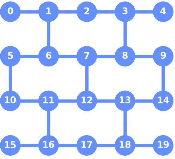
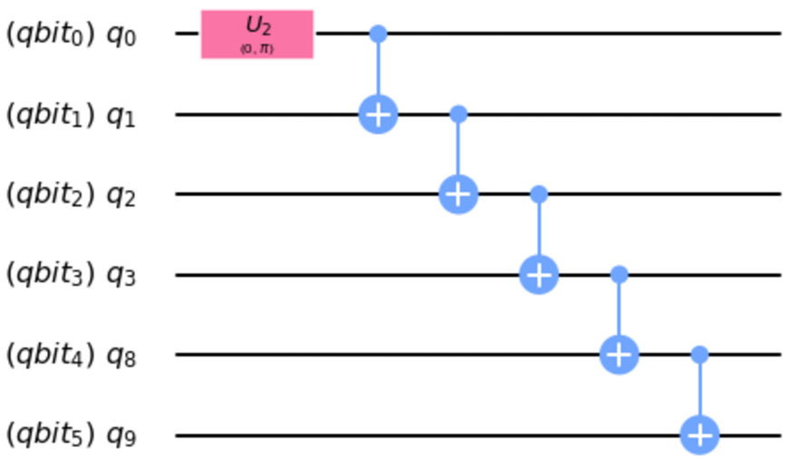
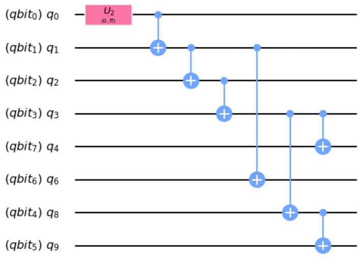
Figure 1: Left panel: Layout connectivity of IBM backend ibmq_boeblingen; Middle and right panels: Circuits used to generate 6-qubit state (left) and 8-qubit GHZ state (right). $qbit$ refers to the quantum registers used in qiskit, and $q$ corresponds to qubits on the real device.

The QST circuits were generated using the tomography module in qiskit-ignis. For complete QST of a $n$-qubits state $3^{n}$ circuits are needed. The result of each circuit is averaged over 8192, 4096 or 2048, for different $n$-qubit scenarios. To mitigate for readout errors, we prepare and measure all of the $2^{n}$ computational basis states in the computation basis to construct a calibration matrix $C$. $C$ has dimension $2^{n}$ by $2^{n}$, where each column vector corresponds to the measured outcome of a prepared basis state. In the ideal case of no readout error, $C$ is an identity matrix. We use $C$ to correct for the measured outcomes of the experiment by minimizing the function:

$$\min_{v^{\text{cal}}\in\mathbb{R}^{d}} \|Cv^{\text{cal}}-v^{\text{meas}}\|^{2} \sum_{i}v^{\text{cal}}_{i}=1,~{}v^{\text{cal}}_{i}\geq 0,\forall i=1,\dots,d$$ subject to (9)

Here $v^{\text{meas}}$ and $v^{\text{cal}}$ are the measured and calibrated outputs, respectively. The minimization problem is then formulated as a convex optimization problem and solved by quadratic programming using the package cvxopt [97].

MiFGD on 6- and 8-qubit real quantum data

We realize two types of quantum states on IBM QPUs, parameterized by the number of qubits $n$ for each case: these are the $\texttt{GHZ}_{-}(n)$ and $\texttt{Hadamard}(n)$ circuits. We collected measurements over all possible Pauli settings by repeating the experiment for each setting a number of times: these are the number of shots for each setting. The (circuit, number of shots) measurement configurations from IBM Quantum devices are summarized in Table 2.

Circuit	# shots
$\texttt{GHZ}_{-}(6)$	2048
$\texttt{GHZ}_{-}(6)$	8192
$\texttt{GHZ}_{-}(8)$	2048
$\texttt{GHZ}_{-}(8)$	4096
$\texttt{Hadamard}(6)$	8192
$\texttt{Hadamard}(8)$	4096

Table 2: QPU settings.

In the Appendix, we provide target error list plots for the evolution of $\|\widehat{\rho}-\rho^{\star}\|_{F}^{2}$ for reconstructing all the settings in Table 2, both for real data and for simulated scenarios. Further, we provide plots that relate the effect of momentum acceleration on the final fidelity observed for these cases. For clarity, in Figure 2, we summarize the efficiency of momentum acceleration, by showing the reconstruction error only for the following settings: $\texttt{maxiters}=1000$, $\eta=10^{-3}$, $\texttt{reltol}=5\times 10^{-4}$, and $\texttt{measpc}=20\%$. In the plots, $\mu=0$ corresponds to the FGD algorithm in [79], $\mu^{\star}$ corresponds to the value obtained through our theory, while we use $\mu\in\left\{\tfrac{1}{8},\tfrac{1}{4},\tfrac{1}{3},\tfrac{3}{4}\right\}$ to study the acceleration effect. For $\mu^{\star}$, per our theory, we follow the rule $\mu^{\star}\approx\varepsilon/2211$ for $\varepsilon\in(0,1]$; see also the Methods section for more details. Note that, in most of the cases, the curve corresponding to $\mu=0$ is hidden behind the curve corresponding to $\mu\approx\mu^{\star}$. We run each QST experiment for $5$ times for random initializations. We record the evolution of the $\|\widehat{\rho}-\rho^{\star}\|_{F}^{2}$ error at each step, and stop when the relative error of successive iterates gets smaller than reltol or the number of iterations exceeds maxiters (whichever happens first). To implement $\texttt{measpc}=20\%$, we follow the description given above Eq. (8) with $m=\texttt{measpc}\cdot d^{2}$.

To highlight the level of noise existing in real quantum data, in Figure 3, we repeat the same setting using the QASM simulator in qiskit-aer. This is a parallel, high performance quantum circuit simulator written in C++ that can support a variety of realistic circuit level noise models.

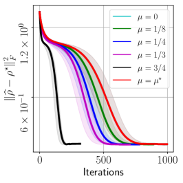
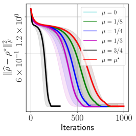
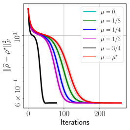
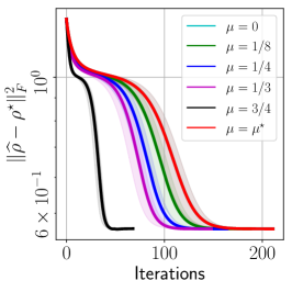
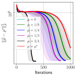
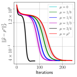
Figure 2: Target error list plots $\|\widehat{\rho}-\rho^{\star}\|_{F}^{2}$ versus method iterations using real IBM QPU data. Top-left: $\texttt{GHZ}_{-}(6)$ with 2048 shots; Top-middle: $\texttt{GHZ}_{-}(6)$ with 8192 shots; Top-right: $\texttt{GHZ}_{-}(8)$ with 2048 shots; Bottom-left: $\texttt{GHZ}_{-}(8)$ with 4096 shots/copies of $\rho^{\star}$; Bottom-middle: $\texttt{Hadamard}(6)$ with 8192 shots; Bottom-right: $\texttt{Hadamard}(8)$ with 4096 shots. All cases have $\texttt{measpc}=20\%$. Shaded area denotes standard deviation around the mean over repeated runs in all cases.

Figure 2 summarizes the performance of our proposal on different $\rho^{\star}$, and for different $\mu$ values on real IBM QPU data. All plots show the evolution of $\|\widehat{\rho}-\rho^{\star}\|_{F}$ across iterations, featuring a steep dive to convergence for the largest value of $\mu$ we tested: we report that we also tested $\mu=0$, which shows only slight worse performances than $\mu^{\star}$. Figure 2 highlights the universality of our approach: its performance is oblivious to the quantum state reconstructed, as long as it satisfies purity or it is close to a pure state. Our method does not require any additional structure assumptions in the quantum state.

To highlight the effect of real noise on the performance of MiFGD, we further plot its performance on the same settings but using measurements coming from an idealized quantum simulator. Figure 3 considers the exact same settings as in Figure 2. It is obvious that MiFGD can achieve better reconstruction performance when data are less erroneous. This also highlights that, in real noisy scenarios, the radius of the convergence region of MiFGD around $\rho^{\star}$ is controlled mostly by the the noise level, rather than by the inclusion of momentum acceleration.

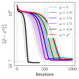
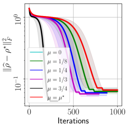
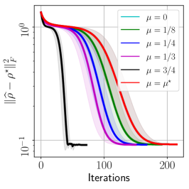
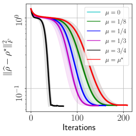
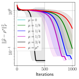
Figure 3: Target error list plots $\|\widehat{\rho}-\rho^{\star}\|_{F}^{2}$ versus method iteration using synthetic IBM’s quantum simulator data. Top-left: $\texttt{GHZ}_{-}(6)$ with 2048 shots; Top-middle: $\texttt{GHZ}_{-}(6)$ with 8192 shots; Top-right: $\texttt{GHZ}_{-}(8)$ with 2048 shots; Bottom-left: $\texttt{GHZ}_{-}(8)$ with 4096 shots; Bottom-middle: $\texttt{Hadamard}(6)$ with 8192 shots; Bottom-right: $\texttt{Hadamard}(8)$ with 4096 shots. All cases have $\texttt{measpc}=20\%$. Shaded area denotes standard deviation around the mean over repeated runs in all cases.

Finally, in Figure 4, we depict the fidelity of $\widehat{\rho}$ achieved using MiFGD, defined as $\text{Tr}\big{(}\rho^{\star}\widehat{\rho}\big{)}$, versus various $\mu$ values and for different circuits $(\rho^{\star})$. Shaded area denotes standard deviation around the mean over repeated runs in all cases. The plots show the significant gap in performance when using real quantum data versus using synthetic simulated data within a controlled environment.

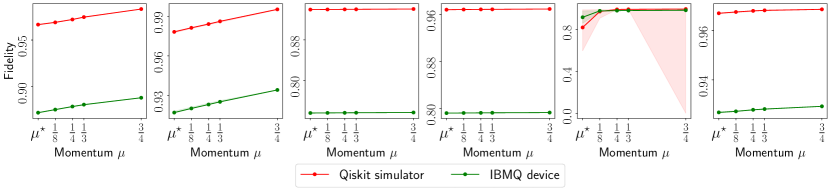
Figure 4: Fidelity list plots where we depict the fidelity of $\widehat{\rho}$ to $\rho^{\star}$. From left to right: $i)$ $\texttt{GHZ}_{-}(6)$ with 2048 shots; $ii)$ $\texttt{GHZ}_{-}(6)$ with 8192 shots; $iii)$ $\texttt{GHZ}_{-}(8)$ with 2048 shots; $iv)$ $\texttt{GHZ}_{-}(8)$ with 4096 shots; $v)$ $\texttt{Hadamard}(6)$ with 8192 shots; $vi)$ $\texttt{Hadamard}(8)$ with 4096 shots. All cases have $\texttt{measpc}=20\%$. Shaded area denotes standard deviation around the mean over repeated runs in all cases.

Performance comparison with full tomography methods in Qiskit

We compare MiFGD with publicly available implementations for QST reconstruction. Two common techniques for QST, included in the qiskit-ignis distribution [81], are: $i)$ the CVXPY fitter method, that uses the CVXPY convex optimization package [26, 5]; and $ii)$ the lstsq method, that uses least-squares fitting [88]. Both methods solve the full tomography problem according to the following expression:

$$\min_{\rho\in\mathbb{C}^{d\times d}} f(\rho):=\tfrac{1}{2}\|\mathcal{A}(\rho)-y\|_{2}^{2}$$ (10)

subject to $$\rho\succeq 0,\texttt{Tr}(\rho)=1.$$

We note that MiFGD is not restricted to “tall” $U$ scenarios to encode PSD and rank constraints: even without rank constraints, one could still exploit the matrix decomposition $\rho=UU^{\dagger}$ to avoid the PSD projection, $\rho\succeq 0$, where $U\in\mathbb{C}^{d\times d}$. For the lstsq fitter method, the putative estimate $\widehat{\rho}$ is rescaled using the method proposed in [88]. For CVXPY, the convex constraint makes the optimization problem a semidefinite programming (SDP) instance. By default, CVXPY calls the SCS solver that can handle all problems (including SDPs) [73, 74]. Further comparison results with matrix factorization techniques from the machine learning community is provided in the Appendix for $n=12$.

The settings we consider for full tomography are the following: $\texttt{GHZ}(n)$, $\texttt{Hadamard}(n)$ and $\texttt{Random}(n)$ quantum states (for $n=3,\dots,8$). We focus on fidelity of reconstruction and computation timings performance between CVXPY, lstsq and MiFGD. We use 100% of the measurements. We experimented with states simulated in QASM and measured taking $2,048$ shots. For MiFGD, we set $\eta=0.001$, $\mu=\tfrac{3}{4}$, and stopping criterion/tolerance $\texttt{reltol}=10^{-5}$. All experiments are run on a Macbook Pro with 2.3 GHz Quad-Core Intel Core i7CPU and 32GB RAM.

The results are shown in Figure 5; higher-dimensional cases are provided in Table 3. Some notable remarks: $i)$ For small-scale scenarios ($n=3,4$), CVXPY and lstsq attain almost perfect fidelity, while being comparable or faster than MiFGD. $ii)$ The difference in performance becomes apparent from $n=6$ and on: while MiFGD attains 98% fidelity in $<5$ seconds, CVXPY and lstsq require up to hundreds of seconds to find a good solution. $iii)$ Finally, while MiFGD gets to high-fidelity solutions in seconds for $n=7,8$, CVXPY and lstsq methods could not finish tomography as their memory usage exceeded the system’s available memory.

It is noteworthy that the reported fidelities for MiFGD are the fidelities at the last iteration, before the stopping criterion is activated, or the maximum number of iterations is exceeded. However, the reported fidelity is not necessarily the best one during the whole execution: for all cases, we observe that MiFGD finds intermediate solutions with fidelity $>99\%$. Though, it is not realistic to assume that the iteration with the best fidelity is known a priori, and this is the reason we report only the final iteration fidelity.

Circuit	Method	Fidelity	Time (secs)
$\texttt{GHZ}(7)$	MiFGD	0.969397	10.6709
$\texttt{Hadamard}(7)$	MiFGD	0.969397	10.4926
$\texttt{Random}(7)$	MiFGD	0.968553	9.59607
All above	lstsq, CVXPY	Memory limit exceeded
$\texttt{GHZ}(8)$	MiFGD	0.940389	35.0666
$\texttt{Hadamard}(8)$	MiFGD	0.940390	37.5331
$\texttt{Random}(8)$	MiFGD	0.942815	36.3251
All above	lstsq, CVXPY	Memory limit exceeded

Table 3: Fidelity of reconstruction and computation timings using 100% of the complete measurements. Rows correspond to combinations of number of qubits (7 $\sim$ 8), synthetic circuit, and tomographic method (MiFGD, Qiskit’s lstsq and CVXPY fitters. 2048 shots per measurement circuit. For MiFGD, $\eta=0.001$, $\mu=\tfrac{3}{4}$, $\texttt{reltol}=10^{-5}$. All experiments are run on a 13” Macbook Pro with 2.3 GHz Quad-Core Intel Core i7 CPU and $32$ GB RAM.

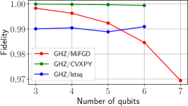
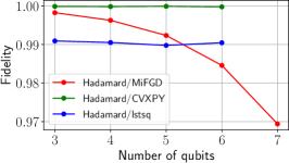
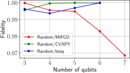
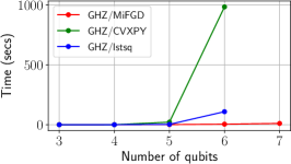
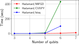
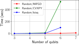
Figure 5: Fidelity versus time plots using synthetic IBM’s quantum simulator data. Left panel: $\texttt{GHZ}_{-}(n)$ for $n=3,4$; Middle panel: $\texttt{Hadamard}_{-}(n)$ for $n=3,4$; Right panel: $\texttt{Random}_{-}(n)$ for $n=3,4$.

Performance comparison of MiFGD with neural-network quantum state tomography

We compare the performance of MiFGD with neural network approaches. Per [93, 12, 94, 31], we model a quantum state with a two-layer Restricted Boltzmann Machine (RBM). RBMs are stochastic neural networks, where each layer contains a number of binary stochastic variables: the size of the visible layer corresponds to the number of input qubits, while the size of the hidden layer is a hyperparameter controlling the representation error. We experiment with three types of RBMs for reconstructing either the positive-real wave function, the complex wave function, or the density matrix of the quantum state. In the first two cases the state is assumed pure while in the last, general mixed quantum states can be represented. We leverage the implementation in QuCumber [12], PositiveRealWaveFunction (PRWF), ComplexWaveFunction (CWF), and DensityMatrix (DM), respectively.

We reconstruct $\texttt{GHZ}(n)$, $\texttt{Hadamard}(n)$ and $\texttt{Random}(n)$ quantum states (for $n=3,\dots,8$), by training PRWF, CWF, and DM neural networks with measurements collected by the QASM Simulator.

For our setting, we consider measpc = 50% and shots = 2048. The set of measurements is presented to the RBM implementation, along with the target positive-real wave function (for PRWF), complex wavefunction (for CWF) or the target density matrix (for DM) in a suitable format for training. We train Hadamard and Random states with 20 epochs, and GHZ state with 100 epochs. We set the number of hidden variables (and also of additional auxilliary variables for DM) to be equal to the number of input variables $n$ and we use $100$ data points for both the positive and the negative phase of the gradient (as per the recommendation for the defaults). We choose $k=10$ contrastive divergence steps and fixed the learning rate to $10$ (per hyperparameter tuning). Lastly, we limit the fitting time of Qucumber methods (excluding data preparation time) to be three hours. To compare to the RBM results, we run MiFGD with $\eta=0.001$, $\mu=\tfrac{3}{4}$, $\texttt{reltol}=10^{-5}$ and using measpc = 50%, keeping previously chosen values for all other hyperparameters.

We report the fidelity of the reconstruction as a function of elapsed training time for $n=3,4$ in Figure 6 for PRWF, CWF, and DM. We observe that for all cases, Qucumber methods are orders of magnitude slower than MiFGD. E.g., for $n=8$, for all three states, CWF and DM did not finish a single epoch in 3 hours, while MiFG achieves high fidelity in less than 30 seconds. For the $\texttt{Hadamard}(n)$ and $\texttt{Random}(n)$, reaching reasonable fidelities is significantly slower for both CWF and DM, while PRWF hardly improves its performance throughout the training. For the GHZ case, CWF and DM also shows non-monotonic behaviors: even after a few thousands of seconds, fidelities have not “stabilized”, while PRWF stabilizes in very low fidelities. In comparison MiFGD is several orders of magnitude faster than both CWF and DM and fidelity smoothly increases to comparable or higher values. Further, in Table 4, we report final fidelities (within the 3 hour time window), and reported times.

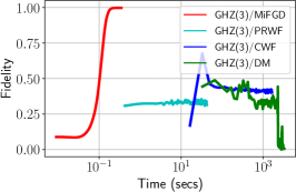
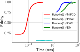
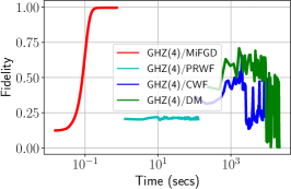
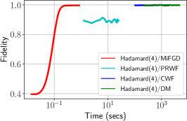
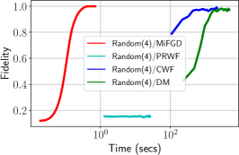
Figure 6: Fidelity versus time plots on MiFGD, PRWF, CWF, and DM, using synthetic IBM’s quantum simulator data. Left panel: $\texttt{GHZ}(n)$ for $n=3,4$; Middle panel: $\texttt{Hadamard}(n)$ for $n=3,4$; Right panel: $\texttt{Random}(n)$ for $n=3,4$.

Circuit		Method
		MiFGD	FGD	PRWF	CWF	DM
$\texttt{GHZ}(3)$	Fidelity	0.997922	0.997857	0.314167	0.401737	0.005389
	Time (secs)	0.348652	1.061421	42.27607	1649.224	3279.118
$\texttt{Hadamard}(3)$	Fidelity	0.997229	0.994191	0.912268	0.997914	0.997222
	Time (secs)	0.706872	2.399405	8.492405	325.7040	656.6696
$\texttt{Random}(3)$	Fidelity	0.991063	0.988746	0.074774	0.997493	0.989754
	Time (secs)	1.447057	3.431218	8.345135	322.4730	640.8185
$\texttt{GHZ}(4)$	Fidelity	0.996029	0.996041	0.204313	0.276491	0.138459
	Time (secs)	0.733128	2.081035	126.2749	10756.87	$>$ 3h
$\texttt{Hadamard}(4)$	Fidelity	0.996078	0.996083	0.894883	0.998071	0.997389
	Time (secs)	0.852895	2.368223	25.15520	2087.540	4613.964
$\texttt{Random}(4)$	Fidelity	0.998850	0.998876	0.152971	0.984164	0.972877
	Time (secs)	0.713302	2.380326	26.18863	2185.091	4802.495
$\texttt{GHZ}(5)$	Fidelity	0.992105	0.992106	0.132725	0.274665	0.005138
	Time (secs)	0.946350	3.287358	395.3379	$>$ 3h	$>$ 3h
$\texttt{Hadamard}(5)$	Fidelity	0.992102	0.992100	0.869603	0.998246	0.996516
	Time (secs)	1.183290	3.895312	79.39444	9319.140	$>$ 3h
$\texttt{Random}(5)$	Fidelity	0.995126	0.995109	0.015913	0.623273	0.086777
	Time (secs)	0.988173	3.407487	79.22450	9275.836	$>$ 3h
$\texttt{GHZ}(6)$	Fidelity	0.984352	0.984340	0.089355	0.437323	0.310067
	Time (secs)	3.829866	13.306954	1167.985	$>$ 3h	$>$ 3h
$\texttt{Hadamard}(6)$	Fidelity	0.984384	0.984377	0.842515	0.990849	0.998077
	Time (secs)	2.500354	8.661999	246.0011	$>$ 3h	$>$ 3h
$\texttt{Random}(6)$	Fidelity	0.989543	0.989536	0.143145	0.784873	0.302534
	Time (secs)	1.991154	7.604232	237.7037	$>$ 3h	$>$ 3h
$\texttt{GHZ}(7)$	Fidelity	0.969174	0.969168	0.058387	0.080648	N/A
	Time (secs)	6.174129	15.895504	3633.082	$>$ 3h	$>$ 3h
$\texttt{Hadamard}(7)$	Fidelity	0.969156	0.969156	0.818174	0.996586	N/A
	Time (secs)	6.324469	16.283301	713.9404	$>$ 3h	$>$ 3h
$\texttt{Random}(7)$	Fidelity	0.967640	0.967619	0.141745	0.06568	N/A
	Time (secs)	6.802577	16.594162	746.2630	$>$ 3h	$>$ 3h
$\texttt{GHZ}(8)$	Fidelity	0.940601	0.940600	0.0400391	N/A	N/A
	Time (secs)	21.16011	36.892739	$>$ 3h	$>$ 3h	$>$ 3h
$\texttt{Hadamard}(8)$	Fidelity	0.940638	0.940638	0.794892	N/A	N/A
	Time (secs)	22.30246	41.472961	2344.796	$>$ 3h	$>$ 3h
$\texttt{Random}(8)$	Fidelity	0.939418	0.939416	0.050521	N/A	N/A
	Time (secs)	22.81059	41.193810	2196.259	$>$ 3h	$>$ 3h

Table 4: Fidelity of reconstruction and computation timings using $\texttt{measpc}=50\%$ and $\texttt{shots}=2048$. Rows correspond to combinations of number of qubits (3 $\sim$ 8), final fidelity within the 3h time limit, and computation time. For MiFGD, $\eta=0.001$, $\mu=\tfrac{3}{4}$, $\texttt{tol}=10^{-5}$. For FGD, $\eta=0.001$, $\texttt{tol}=10^{-5}$. “N/A” indicates that the method could not complete a single epoch in 3 hour training time limit, and thus could not provide any fidelity result. All experiments are run on a NVidia GeForce GTX 1080 TI, $11$GB RAM.

The effect of parallelization

We study the effect of parallelization in running MiFGD. We parallelize the iteration step across a number of processes, that can be either distributed and network connected, or sharing memory in a multicore environment. Our approach is based on Message Passing Interface (MPI) specification [30], which is the lingua franca for interprocess communication in high performance parallel and supercomputing applications. A MPI implementation provides facilities for launching processes organized in a virtual topology and highly tuned primitives for point-to-point and collective communication between them.

We assign to each process a subset of the measurement labels consumed by the parallel computation. At each step, a process first computes the local gradient-based corrections due only to its assigned Pauli monomials and corresponding measurements. These local gradient-based corrections will then $(i)$ need to be communicated, so that they can be added, and $(ii)$ finally, their sum will be shared across all processes to produce a global update for $U$ for next step. We accomplish this structure in MPI using MPI_Allreduce collective communication primitive with MPI_SUM as its reduction operator: the underlying implementation will ensure minimum communication complexity for the operation (e.g. $\log p$ steps for $p$ processes organized in a communication ring) and thus maximum performance. We leverage mpi4py [25] bindings to issue MPI calls in our parallel Python code.

We conducted our parallel experiments on a server equipped with 4 x E7-4850 v2 CPUs @ 2.30GHz (48/96 physical/virtual cores), 256 GB RAM, using shared memory multiprocessing over multiple cores. We experimented with states simulated in QASM and measured taking $8,192$ shots; parallel MiFGD runs with default parameters and using all measurements (measpc=100%). Reported times are wall-clock computation time. These exclude initialization time for all processes to load Pauli monomials and measurements: we here target parallelizing computation proper in MiFGD.

In our first round of experiments, we investigate the scalability of our approach. We vary the number $p$ of parallel processes ($p=1,2,4,8,16,32,48,64,80,96$), collect timings for reconstructing $\texttt{GHZ}(4)$, $\texttt{Random}(6)$ and $\texttt{GHZ}_{-}(8)$ states and report speedups $T_{p}/T_{1}$ we gain from MiFGD in Figure 7(Left panel). We observe that the benefits of parallelization are pronounced for bigger problems (here: $n=8$ qubits) and maximum scalability results when we use all physical cores ($48$ in our platform).

Further, we move to larger problems ($n=10$ qubits: reporting on reconstructing $\texttt{Hadamard}(10)$ state) and focus on the effect parallelization to achieving a given level of fidelity in reconstruction. In Figure 7(Middle panel) we illustrate the fidelity as a function of the time spent in the iteration loop of MiFGD for ($p=8,16,32,48,64$): we observe the smooth path to convergence in all $p$ counts which again minimizes compute time for $p=48$. Note that in this case we use measpc = 10% and $\mu=\frac{1}{4}$.

Finally, in Figure 7(Right panel), we fix the number of processes to $p=48$, in order to minimize compute time and increase the percentage of used measurements to $20\%$ of the total available for $\texttt{Hadamard}(10)$. We vary the acceleration parameter, $\mu=0$ (no acceleration) to $\mu=\frac{1}{4}$ and confirm that we indeed get faster convergence times in the latter case while the fidelity value remains the same (i.e. coinciding upper plateau value in the plots). We can also compare with the previous fidelity versus time plot, where the same $\mu$ but half the measurements are consumed: more measurements translate to faster convergence times (plateau is reached roughly $25\%$ faster; compare the green line with the yellow line in the previous plot).

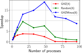
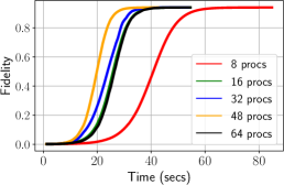
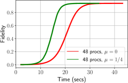
Figure 7: Left panel: Scalability of our approach as we vary the number $p$ of parallel processes. Middle panel: Fidelity function versus time consumed for different number of processes $p$. Right panel: The effect of momentum for a fixed scenario with $\texttt{Hadamard}(10)$ state, $p=48$, and varying momentum from $\mu=0$ to $\mu=\tfrac{1}{4}$.

Discussion

We have introduced the MiFGD algorithm for the factorized form of the low-rank QST problems. We proved that, under certain assumptions on the problem parameters, MiFGD converges linearly to a neighborhood of the optimal solution, whose size depends on the momentum parameter $\mu$, while using acceleration motions in a non-convex setting. We demonstrate empirically, using both simulated and real data, that MiFGD outperforms non-accelerated methods on both the original problem domain and the factorized space, contributing to recent efforts on testing QST algorithms in real quantum data [83]. These results expand on existing work in the literature illustrating the promise of factorized methods for certain low-rank matrix problems. Finally, we provide a publicly available implementation of our approach, compatible to the open-source software Qiskit [81], where we further exploit parallel computations in MiFGD by extending its implementation to enable efficient, parallel execution over shared and distributed memory systems.

Despite our theory does not apply to the Pauli basis measurement directly (i.e., using randomly selected Pauli bases $\Pi_{\alpha}$, does not lead to the $\ell_{2}$-norm RIP), using the data from random Pauli basis measurements directly could provide excellent tomographic reconstruction with MiFGD. Preliminary results suggest that only $O(r\cdot\log d)$ random Pauli bases should be taken for a reconstruction, with the same level of accuracy as with $O(r\cdot d\cdot\log d)$ expectation values of random Pauli matrices. We leave the analysis of our algorithm in this case for future work, along with detailed experiments.

Related Work

Matrix sensing. The problem of low-rank matrix reconstruction from few samples was first studied within the paradigm of convex optimization, using the nuclear norm minimization [82, 60, 64]. The use of non-convex approaches for low-rank matrix recovery—by imposing rank-constraints—has been proposed in [47, 61, 56]. In all these works, the convex and non-convex algorithms involve a full, or at least a truncated, singular value decomposition (SVD) per algorithm iteration. Since SVD can be prohibitive, these methods are limited to relatively small system sizes.

Momentum acceleration methods are used regularly in the convex setting, as well as in machine learning practical scenarios [53, 92, 53, 13, 72, 17, 34]. While momentum acceleration was previously studied in non-convex programming setups, it mostly involve non-convex constraints with a convex objective function [55, 56, 52, 101]; and generic non-convex settings but only considering with the question of whether momentum acceleration leads to fast convergence to a saddle point or to a local minimum, rather than to a global optimum [33, 59, 20, 4].

The factorized version for semi-definite programming was popularized in [18]. Effectively the factorization of a the set of PSD matrices to a product of rectangular matrices results in a non-convex setting. This approach have been heavily studied recently, due to computational and space complexity advantages [46, 21, 102, 103, 96, 78, 80, 89, 14, 15, 79, 32, 43, 57]. None of the works above consider the inclusion and analysis of momentum. Moreover, the Procrustes Flow approach [103, 96] uses certain initializations techniques, and thus relies on multiple SVD computations. Our approach on the other hand uses a single, unique, top-$r$ SVD computation. Comparison results beyond QST are provided in the appendix.

Compressed sensing QST using non-convex optimization. There are only few works that study non-convex optimization in the context of compressed sensing QST. The authors of [86] propose a hybrid algorithm that $i)$ starts with a conjugate-gradient (CG) algorithm in the factored space, in order to get initial rapid descent, and $ii)$ switch over to accelerated first-order methods in the original $\rho$ space, provided one can determine the switch-over point cheaply. Using the multinomial maximum likelihood objective, in the initial CG phase, the Hessian of the objective is computed per iteration (i.e., a $4^{n}{\times}4^{n}$ matrix), along with its eigenvalue decomposition. Such an operation is costly, even for moderate values of qubit number $n$, and heuristics are proposed for its completion. From a theoretical perspective, [86] provide no convergence or convergence rate guarantees.

From a different perspective, [71] relies on spectrum estimation techniques [39, 22] and the Empirical Young Diagram algorithm [8, 51] to prove that $O(rd/\varepsilon)$ copies suffice to obtain an estimate $\hat{\rho}$ that satisfies $\|\hat{\rho}-\rho^{\star}\|_{F}^{2}\leq\varepsilon$; however, to the best of our knowledge, there is no concrete implementation of this technique to compare with respect to scalability.

Ref. [95] proposes an efficient quantum tomography protocol by determining the permutationally invariant part of the quantum state. The authors determine the minimal number of local measurement settings, which scales quadratically with the number of qubits. The paper determines which quantities have to be measured in order to get the smallest uncertainty possible. See [67] for a more recent work on permutationally invariant tomography. The method has been tested in a six-qubit experiment in [85].

Ref. [83] presented an experimental implementation of compressed sensing QST of a $n=7$ qubit system, where only $127$ Pauli basis measurements are available. To achieve recovery in practice, the authors proposed a computationally efficient estimator, based on gradient descent method in the factorized space. The authors of [83] focus on the experimental efficiency of the method, and provide no specific results on the optimization efficiency, neither convergence guarantees of the algorithm. Further, there is no available implementation publicly available.

Similar to [83], Ref. [57] also proposes a non-convex projected gradient decent algorithm that works on the factorized space in the QST setting. The authors prove a rigorous convergence analysis and show that, under proper initialization and step-size, the algorithm is guaranteed to converge to the global minimum of the problem, thus ensuring a provable tomography procedure. Our results extend these results by including acceleration techniques in the factorized space. The key contribution of our work is proving convergence of the proposed algorithm in a linear rate to the global minimum of the problem, under common assumptions. Proving our results required developing a whole set of new techniques, which are not based on a mere extension of existing results.

Compressed sensing QST using convex optimization. The original formulation of compressed sensing QST [38] is based on convex optimization methods, solving the trace-norm minimization, to obtain an estimation of the low-rank state. It was later shown [49] that essentially any convex optimization program can be used to robustly estimate the state. In general, there are two drawbacks in using convex optimization optimization in QST. Firstly, as the dimension of density matrices grow exponentially in the number of qubits, the search space in convex optimization grows exponentially in the number of qubits. Secondly, the optimization requires projection onto the PSD cone at every iteration, which becomes exponentially hard in the number of qubits. We avoid these two drawbacks by working in the factorized space. Using this factorization results in a search space that is substantially smaller than its convex counterpart, and moreover, in a single use of top-$r$ SVD during the entire execution algorithm. Bypassing these drawbacks, together with accelerating motions, allows us to estimate quantum states of larger qubit systems than state-of-the-art algorithms.

Full QST using non-convex optimization. The use of non-convex algorithms in QST was studied in the context of full tomography as well. By “full tomography” we refer to the situation where an informationally complete measurement is performed, so that the input data to the algorithm is of size $4^{n}$. The exponential scaling of the data size restrict the applicability of full tomography to relatively small system sizes. In this setting non-convex algorithms which work in the factored space were studied [10, 77, 99, 36, 91]. Except of the work [36], we are not aware of theoretical results on the convergence of the proposed algorithm due to the presence of spurious local minima. The authors of [36] characterize the local vs. the global behavior of the objective function under the factorization $\rho=UU^{\dagger}$ and discuss how existing methods fail due to improper stopping criteria or due to the lack of algorithmic convergence results. Their work highlights the lack of rigorous convergence results of non-convex algorithms used in full quantum state tomography. There is no available implementation publicly available for these methods as well.

Full QST using convex optimization. Despite the non-scalability of full QST, and the limitation of convex optimization, a lot of research was devoted to this topic. Here, we mention only a few notable results that extend the applicability of full QST using specific techniques in convex optimization. Ref [88] shows that for given measurement schemes the solution for the maximum likelihood is given by a linear inversion scheme, followed by a projection onto the set of density matrices. More recently, the authors of [42] used a combination of the techniques of [88] with the sparsity of the Pauli matrices and the use of GPUs to perform a full QST of 14 qubits. While pushing the limit of full QST using convex optimization, obtaining full tomographic experimental data for more than a dozen qubits is significantly time-intensive. Moreover, this approach is highly centralized, in comparison to our approach that can be distributed. Using the sparsity pattern property of the Pauli matrices and GPUs is an excellent candidate approach to further enhance the performance of non-convex compressed sensing QST.

QST using neural networks. Deep neural networks are ubiquitous, with many applications to science and industry. Recently, [93, 12, 94, 31] show how machine learning and neural networks can be used to perform QST, driven by experimental data. The neural network architecture used is based on restricted Boltzmann machines (RBMs) [90], which feature a visible and a hidden layer of stochastic binary neurons, fully connected with weighted edges. Test cases considered include reconstruction of W state, magnetic observables of local Hamiltonians, the unitary dynamics induced by Hamiltonian evolution. Comparison results are provided in the Main Results section. Alternative approaches include conditional generative adversarial networks (CGANs) [7, 6]: in this case, two dueling neural networks, a generator and a discriminator, learn to generate and identify multi-modal models from data.

QST for Matrix Product States (MPS). This is the case of highly structured quantum states where the state is well-approximated by a MPS of low bond dimension [23, 58]. The idea behind this approach is, in order to overcome exponential bottlenecks in the general QST case, we require highly structured subsets of states, similar to the assumptions made in compressed sensing QST. MPS QST is considered an alternative approach to reduce the computational and storage complexity of QST.

Direct fidelity estimation. Rather than focusing on entrywise estimation of density matrices, the direct fidelity estimation procedure focuses on checking how close is the state of the system to a target state, where closeness is quantified by the fidelity metric. Classic techniques require up to $2^{n}/\epsilon^{4}$ number of samples, where $\epsilon$ denotes the accuracy of the fidelity term, when considering a general quantum state [76, 45], but can be reduced to almost dimensionality-free $1/\epsilon^{2}$ number of samples for specific cases, such as stabilizer states [29, 24, 50]. Shadow tomography is considered as an alternative and generalization of this technique [1, 2]; however, as noted in [45], the procedure in [1, 2] requires exponentially long quantum circuits that act collectively on all the copies of the unknown state stored in a quantum memory, and thus has not been implemented fully on real quantum machines. A recent neural network-based implementation of such indirect QST learning methods is provided here [87].

The work in [76, 45], goes beyond simple fidelity estimation, and utilizes random single qubit rotations to learn a minimal sketch of the unknown quantum state by which one that can predict arbitrary linear function of the state. Such methods constitute a favorable alternative to QST as they do not require number of samples that scale polynomially with the dimension; however, this, in turn, implies that these methods cannot be used in general to estimate the density matrix itself.

Methods

MiFGD algorithm.

  Input: $\mathcal{A}$, $y$, $r$, $\mu$, and $\#$ iterations $J$.

  Set $U_{0}$ randomly or as in  (11).

  Set $Z_{0}=U_{0}$.

  Set $\eta$ as in (12).

  for $i=0$ to $J-1$ do

     $U_{i+1}=Z_{i}-\eta\mathcal{A}^{\dagger}\left(\mathcal{A}(ZZ^{\dagger})-y\right)\cdot Z_{i}$

     $Z_{i+1}=U_{i+1}+\mu\left(U_{i+1}-U_{i}\right)$

  end for

  Output: $\rho=U_{J}U_{J}^{\dagger}$

Algorithm 1 Momentum-Inspired Factored Gradient Descent

Algorithm 1 contains the details of the Momentum-Inspired Factored Gradient Descent. The initial point $U_{0}$ is either randomly selected [15, 80], or set according to Lemma 4 in [57] to:

$$\rho_{0}=U_{0}U_{0}^{\dagger}=\Pi_{\mathcal{C}}\big{(}\tfrac{-1}{1+\delta_{2r}}\cdot\nabla f(0)\big{)}=\tfrac{1}{1+\delta_{2r}}\Pi_{\mathcal{C}}\bigg{(}\sum_{i=1}^{m}y_{i}A_{i}\bigg{)}$$ (11)

where $\Pi_{\mathcal{C}}(\cdot)$ is the projection onto the set of PSD matrices, $\delta_{2r}\in(0,1)$ is the RIP constant and $\nabla f(0)$ denoted the gradient of $f$ evaluated at the all-zero matrix. Since computing the RIP constants is NP-hard, in practice we compute $U_{0}$ through $\rho_{0}=\tfrac{-1}{\widehat{L}}\Pi_{\mathcal{C}}\big{(}\sum_{i=1}^{m}y_{i}A_{i}\big{)}$, where $\widehat{L}\in(1,\nicefrac{{11}}{{10}}]$, see Theorem 2 below. Compared to randomly selecting $U_{0}$, Eq.  11 involves a gradient descent computation and a top-$r$ eigenvalue calculation. As for the step size in algorithm 1, following Lemma 4 below, it is set to

$$\eta=\tfrac{1}{4\left((1+\delta_{2r})\|Z_{0}Z_{0}^{\dagger}\|_{2}+\|\mathcal{A}^{\dagger}\left(\mathcal{A}(Z_{0}Z_{0}^{\dagger})-y\right)\|_{2}\right)},$$ (12)

where $Z_{0}=U_{0}$. Here as well, in practice we replace $\delta_{2r}$ by $\widehat{L}$. The step size $\eta$ remains constant at every iteration step of the algorithm, and requires only two top-eigenvalue computations to calculate the spectral norms $\|Z_{0}Z_{0}^{\dagger}\|_{2}$ and $\|\mathcal{A}^{\dagger}\big{(}\mathcal{A}(Z_{0}Z_{0}^{\dagger}-y\big{)}\|_{2}$. These computations can be efficiently implemented by any off-the-shelf eigenvalue solver, such as the Power Method or the Lanczos method.

We now present the formal convergence theorem, where under certain conditions, MiFGD achieves an accelerated linear rate.

Theorem 2 (Accelerated convergence rate).

Assume that $\mathcal{A}$ satisfies the RIP with constant $\delta_{2r}\leq\nicefrac{{1}}{{10}}$. Let $U_{0}$ and $U_{-1}$ be such that $\min_{R\in\mathcal{O}}\|U_{0}-U^{\star}R\|_{F},~{}\min_{R\in\mathcal{O}}\|U_{-1}-U^{\star}R\|_{F}\leq\tfrac{\sqrt{\sigma_{r}(\rho^{\star})}}{10^{3}\sqrt{\kappa\tau(\rho^{\star})}}$, where $\kappa:=\tfrac{1+\delta_{2r}}{1-\delta_{2r}}$, $\tau(\rho):=\tfrac{\sigma_{1}(\rho)}{\sigma_{r}(\rho)}$ for rank-$r$ $\rho$, and $\sigma_{i}(\rho)$ is the $i$th singular value of $\rho$. Set step size $\eta$ such that

$$\left[1-\left(\tfrac{\sqrt{1+\delta_{2r}}-\sqrt{1-\delta_{2r}}}{(\sqrt{2}+1)\sqrt{1+\delta_{2r}}}\right)^{4}\right]\cdot\tfrac{10}{4\sigma_{r}(\rho^{\star})(1-\delta_{2r})}\leq\eta\leq\tfrac{10}{4\sigma_{r}(\rho^{\star})(1-\delta_{2r})},$$

and the momentum parameter $\mu=\frac{\varepsilon}{2\cdot 10^{3}r\tau(\rho^{\star})\sqrt{\kappa}},$ for user-defined $\varepsilon\in(0,1]$. For $y=\mathcal{A}(\rho^{\star})$ where rank$(\rho^{\star})=r,$ MiFGD returns a solution such that

$$\min_{R\in\mathcal{O}}\|U_{J+1}-U^{\star}R\|_{F} \leq\left(1-\sqrt{\tfrac{1-\delta_{2r}}{1+\delta_{2r}}}\right)^{J+1}\left(\min_{R\in\mathcal{O}}\|U_{0}-U^{\star}R\|_{F}^{2}+\min_{R\in\mathcal{O}}\|U_{-1}-U^{\star}R\|_{F}^{2}\right)^{1/2}$$

$$\hskip 39.83368pt+\xi\cdot|\mu|\cdot\sigma_{1}(\rho^{\star})^{1/2}\cdot r\cdot\left(1-\left(1-\sqrt{\tfrac{1-\delta_{2r}}{1+\delta_{2r}}}\right)^{J+1}\right)\left(1-\sqrt{\tfrac{1-\delta_{2r}}{1+\delta_{2r}}}\right)^{-1}$$

$$\lessapprox\left(1-\sqrt{\tfrac{1-\delta_{2r}}{1+\delta_{2r}}}\right)^{J+1}\left(\min_{R\in\mathcal{O}}\|U_{0}-U^{\star}R\|_{F}^{2}+\min_{R\in\mathcal{O}}\|U_{-1}-U^{\star}R\|_{F}^{2}\right)^{1/2}+O(\mu),$$ (13)

where $\xi=\sqrt{1-\tfrac{4\eta\sigma_{r}(\rho^{\star})(1-\delta_{2r})}{10}}$. That is, the algorithm has an accelerated linear convergence rate in iterate distances up to a constant proportional to the momentum parameter $\mu$.

The interpretation of the theorem is that the right hand side of Eq. (13) depends on the initial distances $\min_{R\in\mathcal{O}}\|U_{0}-U^{\star}R\|_{F}$ and $\min_{R\in\mathcal{O}}\|U_{-1}-U^{\star}R\|_{F}$ as in convex optimization, where $\left(1-\sqrt{\tfrac{1-\delta_{2r}}{1+\delta_{2r}}}\right)$ appear as a contraction constant. In contrast, the contraction factor of vanilla FGD [57] is of the form $\left(1-\frac{1-\delta_{2r}}{1+\delta_{2r}}\right)$, ignoring some constants.

As we assume the sensing map $\mathcal{A}$ satisfies RIP, the condition number of $f$ depends on the RIP constants $\delta$ such that $\frac{L}{\mu}\propto\frac{1+\delta}{1-\delta},$ since the eigenvalues of the Hessian of $f$, $\mathcal{A}^{\dagger}A(\cdot),$ lie between $1-\delta$ and $1+\delta,$ when restricted to low-rank matrices. Hence, MiFGD has better dependency on the (inverse) condition number of $f$ than FGD. Such improvement of the dependency on the condition number is called “acceleration” in convex optimization [70, 20].

Thus, assuming that the initial points $U_{0}$ and $U_{-1}$ are close enough to the optimum, as stated in the theorem, MiFGD decreases its distance to $U^{\star}$ with an accelerated linear rate, up to an “error” level that depends on the momentum parameter $\mu$ and it is bounded by $\frac{1}{2\cdot 10^{3}r\tau(\rho^{\star})\sqrt{\kappa}}$.

Theorem 2 requires a strong assumption on the momentum parameter $\mu$, which depends on quantities that might not be known a priori for general problems. However, we note that for the special case of QST, we know these quantities exactly: $r$ is the rank of density matrix—thus, for pure states this value is equal to $r=1$; $\tau(\rho^{\star})$ is the (rank-restricted) condition number of the density matrix $\rho$—for pure states, $\tau(\rho^{\star})=\tfrac{\sigma_{1}(\rho)}{\sigma_{r}(\rho)}=\tfrac{\sigma_{1}(\rho)}{\sigma_{1}(\rho)}=1$; and, finally, $\kappa$ is the condition number of the sensing map, where, given the constraint $\delta_{2r}\leq\nicefrac{{1}}{{10}}$, leads to the following bound: $\kappa\leq\nicefrac{{11}}{{9}}$. The above lead to a momentum value $\mu\approx\nicefrac{{\varepsilon}}{{2211}}$. However, as we show in the numerical experiments, the theory is conservative; much larger values of $\mu$ lead to stable, improved performance. Finally, the bound on the condition number in Theorem 2 is not strict, and comes out of the analysis we follow; we point the reader to similar assumptions made where $\tau(\rho^{\star})$ is assumed constant $O(1)$ [62].

The detailed proof is provided in the supplementary material. To the best of our knowledge, this is the first proof for momentum-inspired factorization technique, under common assumptions: both regarding the problem setting, and the assumptions made for its completion. The proof differs from state of the art proofs for non-accelerated factored gradient descent: due to the inclusion of the memory term, three different terms –$U_{i+1},U_{i},U_{i-1}$– need to be handled simultaneously. Further, the proof differs from recent proofs on non-convex, but non-factored, gradient descent methods, as in [52]: the distance metric over rotations $\min_{R\in\mathcal{O}}\|Z_{i}-U^{\star}R\|_{F}$, where $Z_{i}$ includes estimates from two steps in history, is not amenable to simple triangle inequality bounds, and a careful analysis is required. The analysis requires the design of two-dimensional dynamical systems, where we require to characterize and bound the eigenvalues of a $2\times 2$ contraction matrix.

Data availability

The empirical results were obtained via synthetic and real experiments; the algorithm’s implementation is available at https://github.com/gidiko/MiFGD.

Competing interests

The authors declare no competing financial or non-financial interests.

Author contribution

All authors have made substantial contributions to the paper: design of the work, drafting the manuscript, final approval and accountability for all aspects of the work.

Appendix

IBM Quantum system experiments: $\texttt{GHZ}_{-}(6)$ circuit, 2048 shots

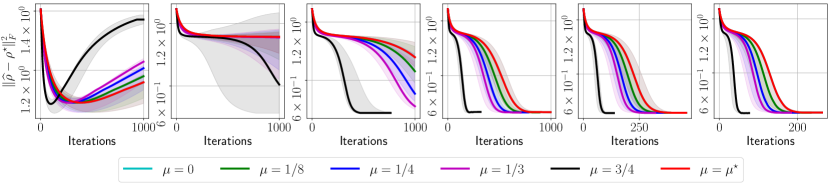
Figure 8: Target error list plots for reconstructing $\texttt{GHZ}_{-}(6)$ circuit using real measurements from IBM Quantum system experiments.

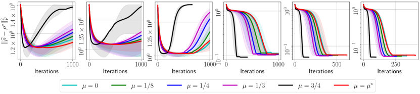
Figure 9: Target error list plots for reconstructing $\texttt{GHZ}_{-}(6)$ circuit using synthetic measurements from IBM’s quantum simulator.

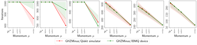
Figure 10: Convergence iteration plots for reconstructing $\texttt{GHZ}_{-}(6)$ circuit using using real measurements from IBM Quantum system experiments and synthetic measurements from Qiskit simulation experiments.

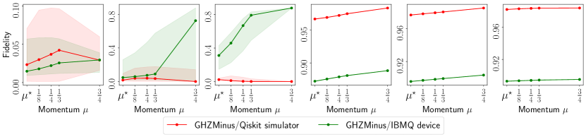
Figure 11: Fidelity list plots for reconstructing $\texttt{GHZ}_{-}(6)$ circuit using using real measurements from IBM Quantum system experiments and synthetic measurements from Qiskit simulation experiments.

IBM Quantum system experiments: $\texttt{GHZ}_{-}(6)$ circuit, 8192 shots

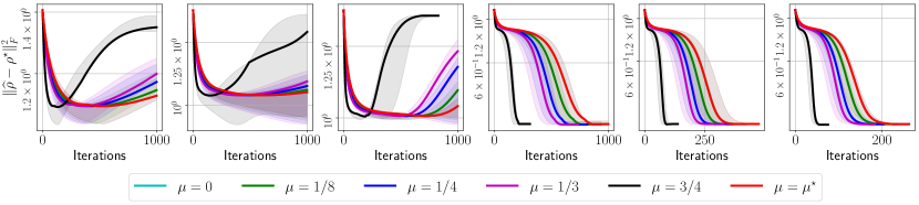
Figure 12: Target error list plots for reconstructing $\texttt{GHZ}_{-}(6)$ circuit using real measurements from IBM Quantum system experiments.

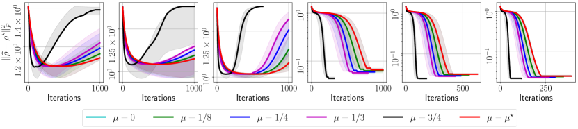
Figure 13: Target error list plots for reconstructing $\texttt{GHZ}_{-}(6)$ circuit using synthetic measurements from IBM’s quantum simulator.

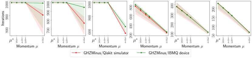
Figure 14: Convergence iteration plots for reconstructing $\texttt{GHZ}_{-}(6)$ circuit using using real measurements from IBM Quantum system experiments and synthetic measurements from Qiskit simulation experiments.

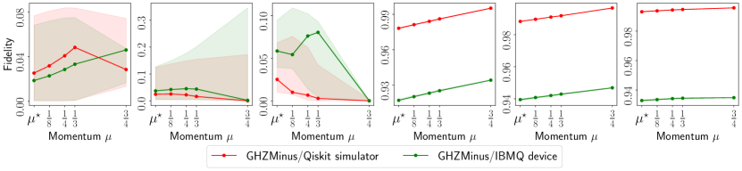
Figure 15: Fidelity list plots for reconstructing $\texttt{GHZ}_{-}(6)$ circuit using using real measurements from IBM Quantum system experiments and synthetic measurements from Qiskit simulation experiments.

IBM Quantum system experiments: $\texttt{GHZ}_{-}(8)$ circuit, 2048 shots

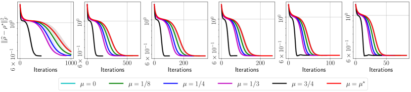
Figure 16: Target error list plots for reconstructing $\texttt{GHZ}_{-}(8)$ circuit using real measurements from IBM Quantum system experiments.

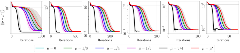
Figure 17: Target error list plots for reconstructing $\texttt{GHZ}_{-}(8)$ circuit using synthetic measurements from IBM’s quantum simulator.

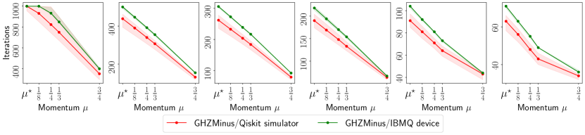
Figure 18: Convergence iteration plots for reconstructing $\texttt{GHZ}_{-}(8)$ circuit using using real measurements from IBM Quantum system experiments and synthetic measurements from Qiskit simulation experiments.

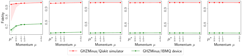
Figure 19: Fidelity list plots for reconstructing $\texttt{GHZ}_{-}(8)$ circuit using using real measurements from IBM Quantum system experiments and synthetic measurements from Qiskit simulation experiments.

IBM Quantum system experiments: $\texttt{GHZ}_{-}(8)$ circuit, 4096 shots

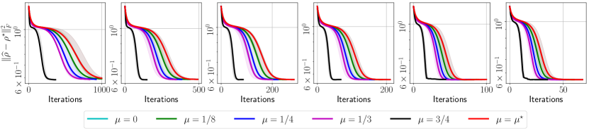
Figure 20: Target error list plots for reconstructing $\texttt{GHZ}_{-}(8)$ circuit using real measurements from IBM Quantum system experiments.

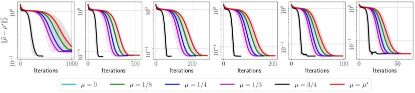
Figure 21: Target error list plots for reconstructing $\texttt{GHZ}_{-}(8)$ circuit using synthetic measurements from IBM’s quantum simulator.

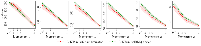
Figure 22: Convergence iteration plots for reconstructing $\texttt{GHZ}_{-}(8)$ circuit using using real measurements from IBM Quantum system experiments and synthetic measurements from Qiskit simulation experiments.

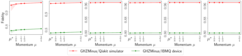
Figure 23: Fidelity list plots for reconstructing $\texttt{GHZ}_{-}(8)$ circuit using using real measurements from IBM Quantum system experiments and synthetic measurements from Qiskit simulation experiments.

IBM Quantum system experiments: $\texttt{Hadamard}(6)$ circuit, 8192 shots

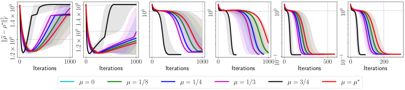
Figure 24: Target error list plots for reconstructing $\texttt{Hadamard}(6)$ circuit using real measurements from IBM Quantum system experiments.

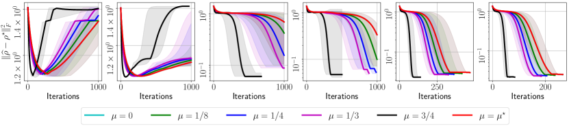
Figure 25: Target error list plots for reconstructing $\texttt{Hadamard}(6)$ circuit using synthetic measurements from IBM’s quantum simulator.

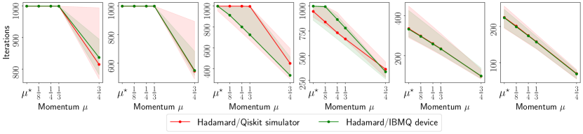
Figure 26: Convergence iteration plots for reconstructing $\texttt{Hadamard}(6)$ circuit using using real measurements from IBM Quantum system experiments and synthetic measurements from Qiskit simulation.

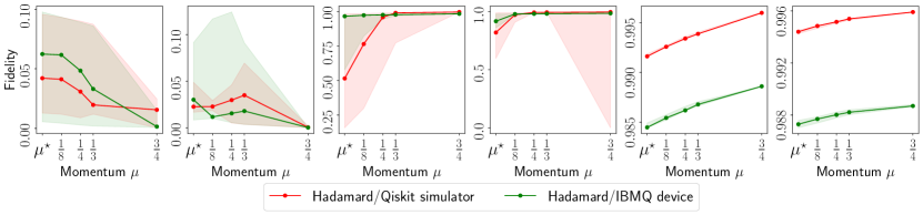
Figure 27: Fidelity list plots for reconstructing $\texttt{Hadamard}(6)$ circuit using using real measurements from IBM Quantum system experiments and synthetic measurements from Qiskit simulation experiments.

IBM Quantum system experiments: $\texttt{Hadamard}(8)$ circuit, 4096 shots

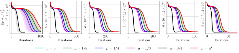
Figure 28: Target error list plots for reconstructing $\texttt{Hadamard}(8)$ circuit using real measurements from IBM Quantum system experiments.

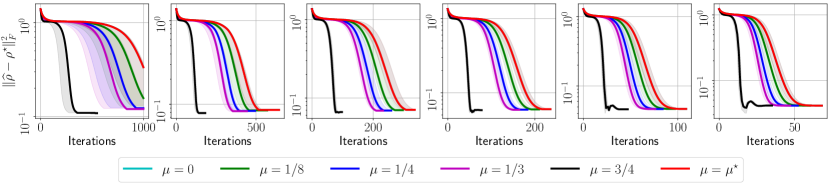
Figure 29: Target error list plots for reconstructing $\texttt{Hadamard}(8)$ circuit using synthetic measurements from IBM’s quantum simulator.

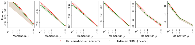
Figure 30: Convergence iteration plots for reconstructing $\texttt{Hadamard}(8)$ circuit using using real measurements from IBM Quantum system experiments and synthetic measurements from Qiskit simulation.

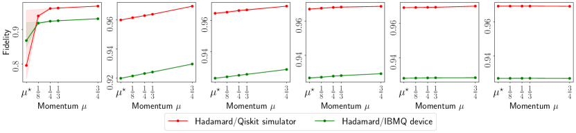
Figure 31: Fidelity list plots for reconstructing $\texttt{Hadamard}(8)$ circuit using using real measurements from IBM Quantum system experiments and synthetic measurements from Qiskit simulation experiments.

Synthetic experiments for $n=12$

We compare MiFGD with $i)$ the Matrix ALPS framework [56], a state of the art projected gradient descent algorithm, and an optimized version of matrix iterative hard thresholding, operating on the full matrix variable $\rho$, with adaptive step size $\eta$ (we note that this algorithm has outperformed most of the schemes that work on the original space $\rho$; see [56]); $ii)$ the plain Procrustes Flow/FGD algorithm [96, 14, 57], where we use the step size as reported in [14], since the later has reported better performance than vanilla Procrustes Flow. We note that the Procrustes Flow/FGD algorithm is similar to our algorithm without acceleration. Further, the original Procrustes Flow/FGD algorithm relies on performing many iterations in the original space $\rho$ as an initialization scheme, which is often prohibitive as the problem dimensions grow. Both for our algorithm and the plain Procrustes Flow/FGD scheme, we use random initialization.

To properly compare the algorithms in the above list, we pre-select a common set of problem parameters. We fix the dimension $d=4096$ (equivalent to $n=12$ qubits), and the rank of the optimal matrix $\rho^{\star}\in\mathbb{R}^{d\times d}$ to be $r=10$ (equivalent to a mixed quantum state reconstruction). Similar behavior has been observed for other values of $r$, and are omitted. We fix the number of observables $m$ to be $m=c\cdot d\cdot r$, where $c\in\{3,5\}$. In all algorithms, we fix the maximum number of iterations to 4000, and we use the same stopping criterion: $\|\rho_{i+1}-\rho_{i}\|_{F}/\|\rho_{i}\|_{F}\leq\texttt{tol}=10^{-3}$. For the implementation of MiFGD, we have used the momentum parameter $\mu=\tfrac{2}{3}$, as well as the theoretical $\mu$ value.

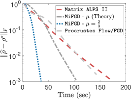
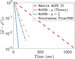
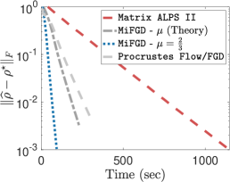
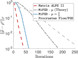
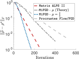
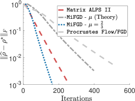
Figure 32: Synthetic example results on low-rank matrix sensing in higher dimensions (equivalent to $n=12$ qubits). Top row: Convergence behavior vs. time elapsed. Bottom row: Convergence behavior vs. number of iterations. Left panel: $c=5$, noiseless case; Center panel: $c=3$, noiseless case; Right panel: $c=5$, noisy case, $\|w\|_{2}=0.01$.

The procedure to generate synthetically the data is as follows: The observations $y$ are set to $y=\mathcal{A}\left(\rho^{\star}\right)+w$ for some noise vector $w$; while the theory holds for the noiseless case, we show empirically that noisy cases are robustly handled by the same algorithm. We use permuted and subsampled noiselets for the linear operator $\mathcal{A}$ [100]. The optimal matrix $\rho^{\star}$ is generated as the multiplication of a tall matrix $U^{\star}\in\mathbb{R}^{d\times r}$ such that $\rho^{\star}=U^{\star}U^{\star\top}$, and $\|\rho^{\star}\|_{F}=1$, without loss of generality. The entries of $U^{\star}$ are drawn i.i.d. from a Gaussian distribution with zero mean and unit variance. In the noisy case, $w$ has the same dimensions with $y$, its entries are drawn from a zero mean Gaussian distribution with norm $\|w\|_{2}=0.01$. The random initialization is defined as $U_{0}$ drawn i.i.d. from a Gaussian distribution with zero mean and unit variance.

The results are shown in Figure 32. Some notable remarks: $i)$ While factorization techniques might take more iterations to converge compared to non-factorized algorithms, the per iteration time complexity is much less, such that overall, factorized gradient descent converges more quickly in terms of total execution time. $ii)$ Our proposed algorithm, even under the restrictive assumptions on acceleration parameter $\mu$, performs better than the non-accelerated factored gradient descent algorithms, such as Procrustes Flow. $iii)$ Our theory is conservative: using a much larger $\mu$ we obtain a faster convergence; the proof for less strict assumptions for $\mu$ is an interesting future direction. In all cases, our findings illustrate the effectiveness of the proposed schemes on different problem configurations.

Asymptotic complexity comparison of lstsq, CVXPY, and MiFGD

We first note that lstsq can be only applied to the case we have a full tomographic set of measurements; this makes lstsq algorithm inapplicable in the compressed sensing scenario, where the number of measurements can be significantly reduced. Yet, we make the comparison by providing information-theoretically complete set of measurements to lstsq and CVXPY, as well as to MiFGD, to highlight the efficiency of our proposed method, even in the scenario that is not exactly intended in our work. Given this, we compare in detail the asymptotic scailing of MiFGD with lstsq and CVXPY below:

• lstsq is based on the computation of eigenvalues/eigenvector pairs (among other steps) of a matrix of size equal to the density matrix we want to reconstruct. Based on our notation, the density matrices are denoted as $\rho$ with dimensions $2^{n}\times 2^{n}$. Here, $n$ is the number of qubits in the quantum system. Standard libraries for eigenvalue/eigenvector calculations, like LAPACK, reduce a Hermitian matrix to tridiagonal form using the Householder method, which takes overall a $O\left((2^{n})^{3}\right)$ computational complexity. The other steps in the lstsq procedure either take constant time, or $O(2^{n})$ complexity. Thus, the actual run-time of an implementation depends on the eigensystem solver that is being used.

• CVXPY is distributed with the open source solvers; for the case of SDP instances, CVXPY utilizes the Splitting Conic Solver (SCS), a general numerical optimization package for solving large-scale convex cone problems. SCS applies Douglas-Rachford splitting to a homogeneous embedding of the quadratic cone program. Based on the PSD constraint, this again involves the computation of eigenvalues/eigenvector pairs (among other steps) of a matrix of size equal to the density matrix we want to reconstruct. This takes overall a $O\left((2^{n})^{3}\right)$ computational complexity, not including the other steps performed within the SCS solver. This is an iterative algorithm that requires such complexity per iteration. Douglas-Rachford splitting methods enjoy $O(\tfrac{1}{\varepsilon})$ convergence rate in general [40, 73, 75]. This leads to a rough $O((2^{n})^{3}\cdot\tfrac{1}{\varepsilon})$ overall iteration complexity.

• For MiFGD, and for sufficiently small momentum value, we require $O(\sqrt{\kappa}\cdot\log(\tfrac{1}{\varepsilon}))$ iterations to get close to the optimal value. Per iteration, MiFGD does not involve any expensive eigensystem solvers, but relies only on matrix-matrix and matrix-vector multiplications. In particular, the main computational complexity per iteration origins from the iteration:

  $$U_{i+1} =Z_{i}-\eta\mathcal{A}^{\dagger}\left(\mathcal{A}(Z_{i}Z_{i}^{\dagger})-y\right)\cdot Z_{i},$$ (14)

  $$Z_{i+1} =U_{i+1}+\mu\left(U_{i+1}-U_{i}\right).$$ (15)

  Here, $U_{i},Z_{i}\in\mathbb{R}^{2^{n}\times r}$ for all $i$. Observe that $\mathcal{A}(Z_{i}Z_{i}^{\dagger})\in\mathbb{R}^{m}$ where each element is computed independently. For an index $j\in[m]$, $(\mathcal{A}(Z_{i}Z_{i}^{\dagger}))_{j}=\texttt{Tr}(A_{j}Z_{i}Z_{i}^{\dagger})$ requires $O((2^{n})^{2}\cdot r)$ complexity, and thus computing $\mathcal{A}(Z_{i}Z_{i}^{\dagger})-y$ requires $O((2^{n})^{2}\cdot r)$ complexity, overall. By definition the adjoing operation $\mathcal{A}^{\dagger}:\mathbb{R}^{m}\rightarrow\mathbb{C}^{2^{n}\times 2^{n}}$ satisfies: $\mathcal{A}^{\dagger}(x)=\sum_{i=1}^{m}x_{i}A_{i}$; thus, the operation $\mathcal{A}^{\dagger}\left(\mathcal{A}(Z_{i}Z_{i}^{\dagger})-y\right)$ is still dominated by $O((2^{n})^{2}\cdot r)$ complexity. Finally, we perform one more matrix-matrix multiplication with $Z_{i}$, which results into an additional $O((2^{n})^{2}\cdot r)$ complexity. The rest of the operations involve adding $2^{n}\times r$ matrices, which does not dominate the overall complexity. Combining the iteration complexity with the per-iteration computational complexity, MiFGD has a $O((2^{n})^{2}\cdot r\cdot\sqrt{\kappa}\cdot\log(\tfrac{1}{\varepsilon}))$ complexity.

Combining the above, we summarize the following complexities:

$$\underbrace{O((2^{n})^{3})}_{\texttt{lstsq}}\quad\quad\text{vs}\quad\quad\underbrace{O((2^{n})^{3}\cdot\tfrac{1}{\varepsilon})}_{\texttt{CVXPY}}\quad\quad\text{vs}\quad\quad\underbrace{O((2^{n})^{2}\cdot r\cdot\sqrt{\kappa}\cdot\log(\tfrac{1}{\varepsilon}))}_{\texttt{MiFGD}}$$

Observe that $i)$ MiFGD has the best dependence on the number of qubits and the ambient dimension of the problem, $2^{n}$; $ii)$ MiFGD applies to cases that lstsq is inapplicable; $iii)$ MiFGD has a better iteration complexity than other iterative algorithms, while has a better polynomial dependency on $2^{n}$.

Detailed proof of Theorem 2

We first denote $U_{+}\equiv U_{i+1}$, $U\equiv U_{i}$, $U_{-}\equiv U_{i-1}$ and $Z\equiv Z_{i}$. Let us start with the following equality. For $R_{Z}\in\mathcal{O}$ as the minimizer of $\min_{R\in\mathcal{O}}\|Z-U^{\star}R\|_{F}$, we have:

$$\|U_{+}-U^{\star}R_{Z}\|_{F}^{2} =\|U_{+}-Z+Z-U^{\star}R_{Z}\|_{F}^{2}$$ (16)

$$=\|U_{+}-Z\|_{F}^{2}+\|Z-U^{\star}R_{Z}\|_{F}^{2}-2\langle U_{+}-Z,U^{\star}R_{Z}-Z\rangle$$ (17)

The proof focuses on how to bound the last part on the right-hand side. By definition of $U_{+}$, we get:

$$\langle U_{+}-Z,U^{\star}R_{Z}-Z\rangle =\left\langle Z-\eta\mathcal{A}^{\dagger}\left(\mathcal{A}(ZZ^{\dagger})-y\right)Z-Z,U^{\star}R_{Z}-Z\right\rangle$$ (18)

$$=\eta\left\langle\mathcal{A}^{\dagger}\left(\mathcal{A}(ZZ^{\dagger})-y\right)Z,Z-U^{\star}R_{Z}\right\rangle$$ (19)

Observe the following:

$$\left\langle\mathcal{A}^{\dagger}\left(\mathcal{A}(ZZ^{\dagger})-y\right)Z,Z-U^{\star}R_{Z}\right\rangle =\left\langle\mathcal{A}^{\dagger}\left(\mathcal{A}(ZZ^{\dagger})-y\right),ZZ^{\dagger}-U^{\star}R_{Z}Z^{\dagger}\right\rangle$$ (20)

$$=\left\langle\mathcal{A}^{\dagger}\left(\mathcal{A}(ZZ^{\dagger})-y\right),ZZ^{\dagger}-\tfrac{1}{2}U^{\star}U^{\star\dagger}+\tfrac{1}{2}U^{\star}U^{\star\dagger}-U^{\star}R_{Z}Z^{\dagger}\right\rangle$$ (21)

$$=\tfrac{1}{2}\left\langle\mathcal{A}^{\dagger}\left(\mathcal{A}(ZZ^{\dagger})-y\right),ZZ^{\dagger}-U^{\star}U^{\star\dagger}\right\rangle$$ (22)

$$\quad\quad+\left\langle\mathcal{A}^{\dagger}\left(\mathcal{A}(ZZ^{\dagger})-y\right),\tfrac{1}{2}(ZZ^{\dagger}+U^{\star}U^{\star\dagger})-U^{\star}R_{Z}Z^{\dagger}\right\rangle$$ (23)

$$=\tfrac{1}{2}\left\langle\mathcal{A}^{\dagger}\left(\mathcal{A}(ZZ^{\dagger})-y\right),ZZ^{\dagger}-U^{\star}U^{\star\dagger}\right\rangle$$ (24)

$$\quad\quad+\tfrac{1}{2}\left\langle\mathcal{A}^{\dagger}\left(\mathcal{A}(ZZ^{\dagger})-y\right),(Z-U^{\star}R_{Z})(Z-U^{\star}R_{Z})^{\dagger}\right\rangle$$ (25)

By Lemmata 5 and 6, we have:

$$\|U_{+}-U^{\star}R_{Z}\|_{F}^{2} =\|U_{+}-Z\|_{F}^{2}+\|Z-U^{\star}R_{Z}\|_{F}^{2}-2\langle U_{+}-Z,U^{\star}R_{Z}-Z\rangle$$ (26)

$$=\eta^{2}\|\mathcal{A}^{\dagger}\left(\mathcal{A}(ZZ^{\dagger})-y\right)Z\|_{F}^{2}+\|Z-U^{\star}R_{Z}\|_{F}^{2}$$ (27)

$$\quad\quad-\eta\left\langle\mathcal{A}^{\dagger}\left(\mathcal{A}(ZZ^{\dagger})-y\right),ZZ^{\dagger}-U^{\star}U^{\star\dagger}\right\rangle$$ (28)

$$\quad\quad\quad\quad-\eta\left\langle\mathcal{A}^{\dagger}\left(\mathcal{A}(ZZ^{\dagger})-y\right),(Z-U^{\star}R_{Z})(Z-U^{\star}R_{Z})^{\dagger}\right\rangle$$ (29)

$$\leq\eta^{2}\|\mathcal{A}^{\dagger}\left(\mathcal{A}(ZZ^{\dagger})-y\right)Z\|_{F}^{2}+\|Z-U^{\star}R_{Z}\|_{F}^{2}$$ (30)

$$\quad\quad-1.0656\eta^{2}\left\|\mathcal{A}^{\dagger}(\mathcal{A}(ZZ^{\dagger})-y)Z\right\|_{F}^{2}-\eta\tfrac{1-\delta_{2r}}{2}\|U^{\star}U^{\star\dagger}-ZZ^{\dagger}\|_{F}^{2}$$ (31)

$$\quad\quad\quad\quad+\eta\Bigg{(}\theta\sigma_{r}(\rho^{\star})\cdot\|Z-U^{\star}R_{Z}\|_{F}^{2}$$ (32)

$$\quad\quad\quad\quad\quad\quad+\tfrac{1}{200}\beta^{2}\cdot\widehat{\eta}\cdot\tfrac{\left(\tfrac{3}{2}+2|\mu|\right)^{2}}{\left(1-\left(\tfrac{3}{2}+2|\mu|\right)\tfrac{1}{10^{3}}\right)^{2}}\cdot\|\mathcal{A}^{\dagger}(\mathcal{A}(ZZ^{\dagger})-y)\cdot Z\|_{F}^{2}\Bigg{)}$$ (33)

Next, we use the following lemma:

Lemma 1.

[96, Lemma 5.4] For any $W,V\in\mathbb{C}^{d\times r}$, the following holds:

$$\|WW^{\dagger}-VV^{\dagger}\|_{F}^{2}\geq 2(\sqrt{2}-1)\cdot\sigma_{r}(VV^{\dagger})\cdot\min_{R\in\mathcal{O}}\|W-VR\|_{F}^{2}.$$ (34)

From Lemma 1, the quantity $\|U^{\star}U^{\star\dagger}-ZZ^{\dagger}\|_{F}^{2}$ satisfies:

$$\|U^{\star}U^{\star\dagger}-ZZ^{\dagger}\|_{F}^{2}\geq 2(\sqrt{2}-1)\cdot\sigma_{r}(\rho^{\star})\cdot\min_{R\in\mathcal{O}}\|Z-U^{\star}R\|_{F}^{2}=2(\sqrt{2}-1)\cdot\sigma_{r}(\rho^{\star})\cdot\|Z-U^{\star}R_{Z}\|_{F}^{2},$$ (35)

which, in our main recursion, results in:

$$\|U_{+}-U^{\star}R_{Z}\|_{F}^{2} \leq\eta^{2}\|\mathcal{A}^{\dagger}\left(\mathcal{A}(ZZ^{\dagger})-y\right)Z\|_{F}^{2}+\|Z-U^{\star}R_{Z}\|_{F}^{2}$$ (36)

$$\quad\quad-1.0656\eta^{2}\left\|\mathcal{A}^{\dagger}(\mathcal{A}(ZZ^{\dagger})-y)Z\right\|_{F}^{2}-\eta(\sqrt{2}-1)(1-\delta_{2r})\sigma_{r}(\rho^{\star})\|Z-U^{\star}R_{Z}\|_{F}^{2}$$ (37)

$$\quad\quad\quad\quad+\eta\Bigg{(}\theta\sigma_{r}(\rho^{\star})\cdot\|Z-U^{\star}R_{Z}\|_{F}^{2}$$ (38)

$$\quad\quad\quad\quad\quad\quad+\tfrac{1}{200}\beta^{2}\cdot\widehat{\eta}\cdot\tfrac{\left(\tfrac{3}{2}+2|\mu|\right)^{2}}{\left(1-\left(\tfrac{3}{2}+2|\mu|\right)\tfrac{1}{10^{3}}\right)^{2}}\cdot\|\mathcal{A}^{\dagger}(\mathcal{A}(ZZ^{\dagger})-y)\cdot Z\|_{F}^{2}\Bigg{)}$$ (39)

$$\stackrel{{\scriptstyle(i)}}{{\leq}}\eta^{2}\|\mathcal{A}^{\dagger}\left(\mathcal{A}(ZZ^{\dagger})-y\right)Z\|_{F}^{2}+\|Z-U^{\star}R_{Z}\|_{F}^{2}$$ (40)

$$\quad\quad-1.0656\eta^{2}\left\|\mathcal{A}^{\dagger}(\mathcal{A}(ZZ^{\dagger})-y)Z\right\|_{F}^{2}-\eta(\sqrt{2}-1)(1-\delta_{2r})\sigma_{r}(\rho^{\star})\|Z-U^{\star}R_{Z}\|_{F}^{2}$$ (41)

$$\quad\quad\quad\quad+\eta\Bigg{(}\theta\sigma_{r}(\rho^{\star})\cdot\|Z-U^{\star}R_{Z}\|_{F}^{2}$$ (42)

$$\quad\quad\quad\quad\quad\quad+\tfrac{1}{200}\beta^{2}\cdot\tfrac{10}{9}\eta\cdot\tfrac{\left(\tfrac{3}{2}+2|\mu|\right)^{2}}{\left(1-\left(\tfrac{3}{2}+2|\mu|\right)\tfrac{1}{10^{3}}\right)^{2}}\cdot\|\mathcal{A}^{\dagger}(\mathcal{A}(ZZ^{\dagger})-y)\cdot Z\|_{F}^{2}\Bigg{)}$$ (43)

$$\stackrel{{\scriptstyle(ii)}}{{=}}\left(1+\tfrac{1}{200}\beta^{2}\cdot\tfrac{10}{9}\cdot\tfrac{\left(\tfrac{3}{2}+2|\mu|\right)^{2}}{\left(1-\left(\tfrac{3}{2}+2|\mu|\right)\tfrac{1}{10^{3}}\right)^{2}}-1.0656\right)\eta^{2}\|\mathcal{A}^{\dagger}(\mathcal{A}(ZZ^{\dagger})-y)\cdot Z\|_{F}^{2}$$ (44)

$$\quad\quad\quad\quad+\left(1+\eta\theta\sigma_{r}(\rho^{\star})-\eta(\sqrt{2}-1)(1-\delta_{2r})\sigma_{r}(\rho^{\star})\right)\|Z-U^{\star}R_{Z}\|_{F}^{2}$$ (45)

where $(i)$ is due to Lemma 4, and $(ii)$ is due to the definition of $U_{+}$.

Under the facts that $\mu=\frac{\sigma_{r}(\rho^{\star})^{1/2}}{10^{3}\sqrt{\kappa\tau(\rho^{\star})}}\cdot\frac{\varepsilon}{4\cdot\sigma_{1}(\rho^{\star})^{1/2}\cdot r}$, for $\varepsilon\in(0,1)$ user-defined, and $\delta_{2r}\leq\tfrac{1}{10}$, the main constant quantities in our proof so far simplify into:

$$\beta=\frac{1+\left(\tfrac{3}{2}+2|\mu|\right)\cdot\tfrac{1}{10^{3}}}{1-\left(\tfrac{3}{2}+2|\mu|\right)\cdot\tfrac{1}{10^{3}}}=1.003,\quad\text{and}\quad\beta^{2}=1.006,$$ (46)

by Corollary 3. Thus:

$$1+\tfrac{1}{200}\beta^{2}\cdot\tfrac{10}{9}\cdot\tfrac{\left(\tfrac{3}{2}+2|\mu|\right)^{2}}{\left(1-\left(\tfrac{3}{2}+2|\mu|\right)\tfrac{1}{10^{3}}\right)^{2}}-1.0656\leq-0.0516,$$ (47)

and our recursion becomes:

$$\|U_{+}-U^{\star}R_{Z}\|_{F}^{2} \leq-0.0516\cdot\eta^{2}\cdot\|\mathcal{A}^{\dagger}(\mathcal{A}(ZZ^{\dagger})-y)\cdot Z\|_{F}^{2}$$ (48)

$$\quad\quad\quad\quad+\left(1+\eta\theta\sigma_{r}(\rho^{\star})-\eta(\sqrt{2}-1)(1-\delta_{2r})\sigma_{r}(\rho^{\star})\right)\|Z-U^{\star}R_{Z}\|_{F}^{2}$$ (49)

Finally,

$$\theta =\tfrac{(1-\delta_{2r})\left(1+\left(\tfrac{3}{2}+2|\mu|\right)\tfrac{1}{10^{3}}\right)^{2}}{10^{3}}+(1+\delta_{2r})\left(2+\left(\tfrac{3}{2}+2|\mu|\right)\cdot\tfrac{1}{10^{3}}\right)\left(\tfrac{3}{2}+2|\mu|\right)\cdot\tfrac{1}{10^{3}}$$ (50)

$$\stackrel{{\scriptstyle(i)}}{{=}}(1-\delta_{2r})\cdot\left(\tfrac{\left(1+(\tfrac{3}{2}+2|\mu|)\tfrac{1}{10^{3}}\right)^{2}}{10^{3}}+\kappa\left(2+\left(\tfrac{3}{2}+2|\mu|\right)\cdot\tfrac{1}{10^{3}}\right)\left(\tfrac{3}{2}+2|\mu|\right)\cdot\tfrac{1}{10^{3}}\right)$$ (51)

$$\leq 0.0047\cdot(1-\delta_{2r}).$$ (52)

where $(i)$ is by the definition of $\kappa:=\tfrac{1+\delta_{2r}}{1-\delta_{2r}}\leq 1.223$ for $\delta_{2r}\leq\tfrac{1}{10}$, by assumption. Combining the above in our main inequality, we obtain:

$$\|U_{+}-U^{\star}R_{Z}\|_{F}^{2} \leq-0.0516\cdot\eta^{2}\cdot\|\mathcal{A}^{\dagger}(\mathcal{A}(ZZ^{\dagger})-y)\cdot Z\|_{F}^{2}$$

$$\quad\quad\quad\quad+\left(1+\eta\sigma_{r}(\rho^{\star})(1-\delta_{2r})\cdot(0.0047-\sqrt{2}+1)\right)\|Z-U^{\star}R_{Z}\|_{F}^{2}$$

$$\leq\left(1-\tfrac{4\eta\sigma_{r}(\rho^{\star})(1-\delta_{2r})}{10}\right)\|Z-U^{\star}R_{Z}\|_{F}^{2}$$ (53)

Taking square root on both sides, we obtain:

$$\|U_{+}-U^{\star}R_{Z}\|_{F} \leq\sqrt{1-\tfrac{4\eta\sigma_{r}(\rho^{\star})(1-\delta_{2r})}{10}}\cdot\|Z-U^{\star}R_{Z}\|_{F}$$ (54)

Let us define $\xi=\sqrt{1-\tfrac{4\eta\sigma_{r}(\rho^{\star})(1-\delta_{2r})}{10}}$. Using the definitions $Z=U+\mu(U-U_{-})$ and $R_{Z}\in\arg\min\limits_{R\in\mathcal{O}}\|Z-U^{\star}R\|_{F}$, we get

$$\|U_{+}-U^{\star}R_{Z}\|_{F} \leq\xi\cdot\min_{R\in\mathcal{O}}\|Z-U^{\star}R\|_{F}=\xi\cdot\min_{R\in\mathcal{O}}\|U+\mu(U-U_{-})-U^{\star}R\|_{F}$$

$$=\xi\cdot\min_{R\in\mathcal{O}}\|U+\mu\left(U-U_{-}\right)-(1-\mu+\mu)U^{\star}R\|_{F}$$

$$\stackrel{{\scriptstyle(i)}}{{\leq}}\xi\cdot|1+\mu|\cdot\min_{R\in\mathcal{O}}\|U-U^{\star}R\|_{F}+\xi\cdot|\mu|\cdot\min_{R\in\mathcal{O}}\|U_{-}-U^{\star}R\|_{F}+\xi\cdot|\mu|\cdot r\sigma_{1}(\rho^{\star})^{1/2}$$

where $(i)$ follows from steps similar to those in Lemma 3. Further observe that $\min_{R\in\mathcal{O}}\|U_{+}-U^{\star}R\|_{F}\leq\|U_{+}-U^{\star}R_{Z}\|_{F}$, thus leading to:

$$\min_{R\in\mathcal{O}}\|U_{+}-U^{\star}R\|_{F}\leq\xi\cdot|1+\mu|\cdot\min_{R\in\mathcal{O}}\|U-U^{\star}R\|_{F}+\xi\cdot|\mu|\cdot\min_{R\in\mathcal{O}}\|U_{-}-U^{\star}R\|_{F}+\xi\cdot|\mu|\cdot r\sigma_{1}(\rho^{\star})^{1/2}$$ (55)

Including two subsequent iterations in a single two-dimensional first-order system, we get the following characterization:

$$\begin{bmatrix}\min_{R\in\mathcal{O}}\|U_{i+1}-U^{\star}R\|_{F}\\ \min_{R\in\mathcal{O}}\|U_{i}-U^{\star}R\|_{F}\end{bmatrix} \leq\begin{bmatrix}\xi\cdot|1+\mu|&\xi\cdot|\mu|\\ 1&0\end{bmatrix}\cdot\begin{bmatrix}\min_{R\in\mathcal{O}}\|U_{i}-U^{\star}R\|_{F}\\ \min_{R\in\mathcal{O}}\|U_{i-1}-U^{\star}R\|_{F}\end{bmatrix}$$ (56)

$$\quad\quad\quad\quad+\begin{bmatrix}1\\ 0\end{bmatrix}\cdot\xi\cdot|\mu|\cdot\sigma_{1}(\rho^{\star})^{1/2}\cdot r.$$ (57)

Now, let $x_{j}=\min_{R\in\mathcal{O}}\|U_{j}-U^{\star}R\|_{F}$. Then, we can write the above relation as

$$\begin{bmatrix}x_{i+1}\\ x_{i}\end{bmatrix} \leq\underbrace{\begin{bmatrix}\xi\cdot|1+\mu|&\xi\cdot|\mu|\\ 1&0\end{bmatrix}}_{:=A}\cdot\begin{bmatrix}x_{i}\\ x_{i-1}\end{bmatrix}+\begin{bmatrix}1\\ 0\end{bmatrix}\cdot\xi\cdot|\mu|\cdot\sigma_{1}(\rho^{\star})^{1/2}\cdot r,$$

where we denote the “contraction matrix” by $A$. Taking norms on both sides, we get

$$\left\|\begin{bmatrix}x_{i+1}\\ x_{i}\end{bmatrix}\right\|_{2} \leq\left\|A\cdot\begin{bmatrix}x_{i}\\ x_{i-1}\end{bmatrix}+\begin{bmatrix}1\\ 0\end{bmatrix}\cdot\xi\cdot|\mu|\cdot\sigma_{1}(\rho^{\star})^{1/2}\cdot r\right\|_{2}$$

$$\stackrel{{\scriptstyle(i)}}{{\leq}}\left\|A\cdot\begin{bmatrix}x_{i}\\ x_{i-1}\end{bmatrix}\right\|_{2}+\left\|\begin{bmatrix}1\\ 0\end{bmatrix}\cdot\xi\cdot|\mu|\cdot\sigma_{1}(\rho^{\star})^{1/2}\cdot r\right\|_{2}$$

$$\stackrel{{\scriptstyle(ii)}}{{\leq}}\left\|A\right\|_{2}\cdot\left\|\begin{bmatrix}x_{i}\\ x_{i-1}\end{bmatrix}\right\|_{2}+\left\|\begin{bmatrix}1\\ 0\end{bmatrix}\cdot\xi\cdot|\mu|\cdot\sigma_{1}(\rho^{\star})^{1/2}\cdot r\right\|_{2},$$ (58)

where $(i)$ is by triangle inequality, and $(ii)$ is by Cauchy–Schwarz inequality.

Therefore, the convergence rate will be determined by the (maximum) eigenvalue of the contraction matrix $A$, which is given by

$$\lambda_{1,2}=\frac{\xi\cdot|1+\mu|}{2}\pm\sqrt{\frac{\xi^{2}(1+\mu)^{2}}{4}+\xi\cdot|\mu|}\stackrel{{\scriptstyle(i)}}{{\implies}}\max\{\lambda_{1},\lambda_{2}\}=\lambda_{1}=\frac{\xi\cdot|1+\mu|}{2}+\sqrt{\frac{\xi^{2}(1+\mu)^{2}}{4}+\xi\cdot|\mu|},$$

where $(i)$ follows since every term in $\lambda_{1,2}$ is positive.

To show accelerated convergence rate, we want the above eigenvalue (which determines the convergence rate) to be bounded by $1-\sqrt{\tfrac{1-\delta_{2r}}{1+\delta_{2r}}}$. To show this, first note that this term is bounded above as follows:

$$\lambda_{1}=\frac{\xi\cdot|1+\mu|}{2}+\sqrt{\frac{\xi^{2}(1+\mu)^{2}}{4}+\xi\cdot|\mu|} \stackrel{{\scriptstyle(i)}}{{\leq}}\xi+\sqrt{\xi^{2}+\xi}$$

$$\stackrel{{\scriptstyle(ii)}}{{\leq}}\xi+\sqrt{2\xi}$$

$$\stackrel{{\scriptstyle(ii)}}{{\leq}}(\sqrt{2}+1)\sqrt{\xi},$$

where $(i)$ is by the conventional bound on momentum: $0<\mu<1$, and $(ii)$ is by the relation $\xi^{2}\leq\xi\leq\sqrt{\xi}$ for $0\leq\xi\leq 1$. Therefore, to show the accelerated rate of convergence, we want the following relation to hold:

$$(\sqrt{2}+1)\sqrt{\xi}\leq 1-\sqrt{\tfrac{1-\delta_{2r}}{1+\delta_{2r}}}\iff\sqrt{\xi}\leq\frac{\sqrt{1+\delta_{2r}}-\sqrt{1-\delta_{2r}}}{(\sqrt{2}+1)\sqrt{1+\delta_{2r}}}.$$ (59)

Recalling our definition of $\xi=\sqrt{1-\tfrac{4\eta\sigma_{r}(\rho^{\star})(1-\delta_{2r})}{10}}$, the problem boils down to choosing the right step size $\eta$ such that the above inequality on $\xi$ in Eq. (59) is satisfied. With simple algebra, we can show the following lower bound on $\eta$:

$$\left[1-\left(\frac{\sqrt{1+\delta_{2r}}-\sqrt{1-\delta_{2r}}}{(\sqrt{2}+1)\sqrt{1+\delta_{2r}}}\right)^{4}\right]\cdot\frac{10}{4\sigma_{r}(\rho^{\star})(1-\delta_{2r})}\leq\eta$$

Finally, the argument inside the $\sqrt{\cdot}$ term of $\xi=\sqrt{1-\tfrac{4\eta\sigma_{r}(\rho^{\star})(1-\delta_{2r})}{10}}>0$ has to be non-negative, yielding the following upper bound on $\eta$:

$$\eta\leq\frac{10}{4\sigma_{r}(\rho^{\star})(1-\delta_{2r})}.$$

Combining two inequalities, and noting that the term $\left[1-\left(\frac{\sqrt{1+\delta_{2r}}-\sqrt{1-\delta_{2r}}}{(\sqrt{2}+1)\sqrt{1+\delta_{2r}}}\right)^{4}\right]$ is bounded above by 1, we arrive at the following bound on $\eta$:

$$\left[1-\left(\frac{\sqrt{1+\delta_{2r}}-\sqrt{1-\delta_{2r}}}{(\sqrt{2}+1)\sqrt{1+\delta_{2r}}}\right)^{4}\right]\cdot\frac{10}{4\sigma_{r}(\rho^{\star})(1-\delta_{2r})}\leq\eta\leq\frac{10}{4\sigma_{r}(\rho^{\star})(1-\delta_{2r})}.$$ (60)

In sum, for the specific $\eta$ satisfying the above bound, we have shown that

$$\lambda_{1}=\frac{\xi\cdot|1+\mu|}{2}+\sqrt{\frac{\xi^{2}(1+\mu)^{2}}{4}+\xi\cdot|\mu|}\leq 1-\sqrt{\frac{1-\delta_{2r}}{1+\delta_{2r}}}$$

Above translates our original recursion in (58) as:

$$\left\|\begin{bmatrix}x_{i+1}\\ x_{i}\end{bmatrix}\right\|_{2} \leq\left\|A\right\|_{2}\cdot\left\|\begin{bmatrix}x_{i}\\ x_{i-1}\end{bmatrix}\right\|_{2}+\left\|\begin{bmatrix}1\\ 0\end{bmatrix}\cdot\xi\cdot|\mu|\cdot\sigma_{1}(\rho^{\star})^{1/2}\cdot r\right\|_{2}$$

$$\leq\left(1-\sqrt{\tfrac{1-\delta_{2r}}{1+\delta_{2r}}}\right)\cdot\left\|\begin{bmatrix}x_{i}\\ x_{i-1}\end{bmatrix}\right\|_{2}+\left\|\begin{bmatrix}1\\ 0\end{bmatrix}\cdot\xi\cdot|\mu|\cdot\sigma_{1}(\rho^{\star})^{1/2}\cdot r\right\|_{2}$$

$$=\left(1-\sqrt{\tfrac{1-\delta_{2r}}{1+\delta_{2r}}}\right)\cdot\left\|\begin{bmatrix}x_{i}\\ x_{i-1}\end{bmatrix}\right\|_{2}+\xi\cdot|\mu|\cdot\sigma_{1}(\rho^{\star})^{1/2}\cdot r,$$ (61)

where the last equality is by the definition of $\ell_{2}$-norm.

Unrolling the recursion in Eq. (61) for $J$ iterations, we get

$$\left\|\begin{bmatrix}x_{J+1}\\ x_{J}\end{bmatrix}\right\|_{2} \leq\left(1-\sqrt{\tfrac{1-\delta_{2r}}{1+\delta_{2r}}}\right)^{J+1}\left\|\begin{bmatrix}x_{0}\\ x_{-1}\end{bmatrix}\right\|_{2}+\xi\cdot|\mu|\cdot\sigma_{1}(\rho^{\star})^{1/2}\cdot r\cdot\sum_{i=0}^{J}\left(1-\sqrt{\tfrac{1-\delta_{2r}}{1+\delta_{2r}}}\right)^{i}$$

$$=\left(1-\sqrt{\tfrac{1-\delta_{2r}}{1+\delta_{2r}}}\right)^{J+1}\left\|\begin{bmatrix}x_{0}\\ x_{-1}\end{bmatrix}\right\|_{2}+\xi\cdot|\mu|\cdot\sigma_{1}(\rho^{\star})^{1/2}\cdot r\cdot\left(1-\left(1-\sqrt{\tfrac{1-\delta_{2r}}{1+\delta_{2r}}}\right)^{J+1}\right)\left(1-\sqrt{\tfrac{1-\delta_{2r}}{1+\delta_{2r}}}\right)^{-1}$$

$$=\left(1-\sqrt{\tfrac{1-\delta_{2r}}{1+\delta_{2r}}}\right)^{J+1}\left\|\begin{bmatrix}x_{0}\\ x_{-1}\end{bmatrix}\right\|_{2}+O(\mu)$$

Finally, computing the $\ell_{2}$-norm explicitly and resubstituting $x_{j}=\min_{R\in\mathbb{O}}\|U_{j}-U^{\star}R\|_{F}$, we get

$$\min_{R\in\mathcal{O}}\|U_{J+1}-U^{\star}R\|_{F} \leq\left(1-\sqrt{\tfrac{1-\delta_{2r}}{1+\delta_{2r}}}\right)^{J+1}\left(\min_{R\in\mathcal{O}}\|U_{0}-U^{\star}R\|_{F}^{2}+\min_{R\in\mathcal{O}}\|U_{-1}-U^{\star}R\|_{F}^{2}\right)^{1/2}+O(\mu).$$

Supporting lemmata

In this section, we present a series of lemmata, used for the main result of the paper.

Lemma 2.

Let $U\in\mathbb{C}^{d\times r}$ and $U^{\star}\in\mathbb{C}^{d\times r}$, such that $\|U-U^{\star}R\|_{F}\leq\tfrac{\sigma_{r}(\rho^{\star})^{1/2}}{10^{3}\sqrt{\kappa\tau(\rho^{\star})}}$ for some $R\in\mathcal{O}$, where $\rho^{\star}=U^{\star}U^{\star\dagger}$, $\kappa:=\tfrac{1+\delta_{2r}}{1-\delta_{2r}}>1$, for $\delta_{2r}\leq\tfrac{1}{10}$, and $\tau(\rho^{\star}):=\tfrac{\sigma_{1}(\rho^{\star})}{\sigma_{r}(\rho^{\star})}>1$. Then:

$$\sigma_{1}(\rho^{\star})^{1/2}\left(1-\tfrac{1}{10^{3}}\right) \leq\sigma_{1}(U)\leq\sigma_{1}(\rho^{\star})^{1/2}\left(1+\tfrac{1}{10^{3}}\right)$$ (62)

$$\sigma_{r}(\rho^{\star})^{1/2}\left(1-\tfrac{1}{10^{3}}\right) \leq\sigma_{r}(U)\leq\sigma_{r}(\rho^{\star})^{1/2}\left(1+\tfrac{1}{10^{3}}\right)$$ (63)

Proof.

By the fact $\|\cdot\|_{2}\leq\|\cdot\|_{F}$ and using Weyl’s inequality for perturbation of singular values [41, Theorem 3.3.16], we have:

$$\left|\sigma_{i}(U)-\sigma_{i}(U^{\star})\right|\leq\tfrac{\sigma_{r}(\rho^{\star})^{1/2}}{10^{3}\sqrt{\kappa\tau(\rho^{\star})}}\leq\tfrac{\sigma_{r}(\rho^{\star})^{1/2}}{10^{3}},\quad 1\leq i\leq r.$$ (64)

Then,

$$-\tfrac{\sigma_{r}(\rho^{\star})^{1/2}}{10^{3}} \leq\sigma_{1}(U)-\sigma_{1}(U^{\star})\leq\tfrac{\sigma_{r}(\rho^{\star})^{1/2}}{10^{3}}\Rightarrow$$ (65)

$$\sigma_{1}(\rho^{\star})^{1/2}-\tfrac{\sigma_{r}(\rho^{\star})^{1/2}}{10^{3}} \leq\sigma_{1}(U)\leq\sigma_{1}(\rho^{\star})^{1/2}+\tfrac{\sigma_{r}(\rho^{\star})^{1/2}}{10^{3}}\Rightarrow$$ (66)

$$\sigma_{1}(\rho^{\star})^{1/2}\left(1-\tfrac{1}{10^{3}}\right) \leq\sigma_{1}(U)\leq\sigma_{1}(\rho^{\star})^{1/2}\left(1+\tfrac{1}{10^{3}}\right).$$ (67)

Similarly:

$$-\tfrac{\sigma_{r}(\rho^{\star})^{1/2}}{10^{3}} \leq\sigma_{r}(U)-\sigma_{r}(U^{\star})\leq\tfrac{\sigma_{r}(\rho^{\star})^{1/2}}{10^{3}}\Rightarrow$$ (68)

$$\sigma_{r}(\rho^{\star})^{1/2}-\tfrac{\sigma_{r}(\rho^{\star})^{1/2}}{10^{3}} \leq\sigma_{r}(U)\leq\sigma_{r}(\rho^{\star})^{1/2}+\tfrac{\sigma_{r}(\rho^{\star})^{1/2}}{10^{3}}\Rightarrow$$ (69)

$$\sigma_{r}(\rho^{\star})^{1/2}\left(1-\tfrac{1}{10^{3}}\right) \leq\sigma_{r}(U)\leq\sigma_{r}(\rho^{\star})^{1/2}\left(1+\tfrac{1}{10^{3}}\right).$$ (70)

In the above, we used the fact that $\sigma_{i}(U^{\star})=\sigma_{i}(\rho^{\star})^{1/2}$, for all $i$, and the fact that $\sigma_{i}(\rho^{\star})^{1/2}\geq\sigma_{j}(\rho^{\star})^{1/2}$, for $i\leq j$. ∎

Lemma 3.

Let $U\in\mathbb{C}^{d\times r},U_{-}\in\mathbb{C}^{d\times r}$, and $U^{\star}\in\mathbb{C}^{d\times r}$, such that $\min_{R\in\mathcal{O}}\|U-U^{\star}R\|_{F}\leq\tfrac{\sigma_{r}(\rho^{\star})^{1/2}}{10^{3}\sqrt{\kappa\tau(\rho^{\star})}}$  and  $\min_{R\in\mathcal{O}}\|U_{-}-U^{\star}R\|_{F}\leq\tfrac{\sigma_{r}(\rho^{\star})^{1/2}}{10^{3}\sqrt{\kappa\tau(\rho^{\star})}}$, where $\rho^{\star}=U^{\star}U^{\star\dagger}$, and $\kappa:=\tfrac{1+\delta_{2r}}{1-\delta_{2r}}>1$, for $\delta_{2r}\leq\tfrac{1}{10}$, and $\tau(\rho^{\star}):=\tfrac{\sigma_{1}(\rho^{\star})}{\sigma_{r}(\rho^{\star})}>1$. Set the momentum parameter as $\mu=\frac{\sigma_{r}(\rho^{\star})^{1/2}}{10^{3}\sqrt{\kappa\tau(\rho^{\star})}}\cdot\frac{\varepsilon}{4\cdot\sigma_{1}(\rho^{\star})^{1/2}\cdot r}$, for $\varepsilon\in(0,1)$ user-defined. Then,

$$\|Z-U^{\star}R_{Z}\|_{F}\leq\left(\tfrac{3}{2}+2|\mu|\right)\cdot\tfrac{\sigma_{r}(\rho^{\star})^{1/2}}{10^{3}\sqrt{\kappa\tau(\rho^{\star})}}.$$ (71)

Proof.

Let $R_{U}\in\arg\min_{R\in\mathcal{O}}\|U-U^{\star}\|_{F}$ and $R_{U_{-}}\in\arg\min_{R\in\mathcal{O}}\|U_{-}-U^{\star}R\|_{F}$. By the definition of the distance function:

$$\|Z-U^{\star}R_{Z}\|_{F} =\min_{R\in\mathcal{O}}\|Z-U^{\star}R\|_{F}=\min_{R\in\mathcal{O}}\|U+\mu(U-U_{-})-U^{\star}R\|_{F}$$ (72)

$$=\min_{R\in\mathcal{O}}\|U+\mu(U-U_{-})-(1-\mu+\mu)U^{\star}R\|_{F}$$ (73)

$$\leq|1+\mu|\cdot\|U-U^{*}R_{U}\|_{F}+|\mu|\cdot||U_{-}-U^{*}R_{U_{-}}||_{F}$$ (74)

$$=|1+\mu|\cdot\|U-U^{*}R_{U}\|_{F}+|\mu|\cdot\|U_{-}-U^{*}R_{U}-U^{*}R_{U_{-}}+U^{*}R_{U_{-}}\|_{F}$$ (75)

$$=|1+\mu|\cdot\|U-U^{*}R_{U}\|_{F}+|\mu|\cdot\|(U_{-}-U^{*}R_{U_{-}})+U^{*}(R_{U_{-}}-R_{U})\|_{F}$$ (76)

$$\leq|1+\mu|\cdot\min_{R\in\mathcal{O}}\|U-U^{\star}R\|_{F}+|\mu|\cdot\min_{R\in\mathcal{O}}\|U_{-}-U^{\star}R\|_{F}+|\mu|\cdot\|U^{\star}(R_{U}-R_{U_{-}})\|_{F}$$ (77)

$$\leq|1+\mu|\cdot\min_{R\in\mathcal{O}}\|U-U^{\star}R\|_{F}+|\mu|\cdot\min_{R\in\mathcal{O}}\|U_{-}-U^{\star}R\|_{F}+2|\mu|\cdot\sigma_{1}(\rho^{\star})^{1/2}r$$ (78)

$$\stackrel{{\scriptstyle(i)}}{{\leq}}\left(\tfrac{3}{2}+2|\mu|\right)\cdot\tfrac{\sigma_{r}(\rho^{\star})^{1/2}}{10^{3}\sqrt{\kappa\tau(\rho^{\star})}}$$ (79)

where $(i)$ is due to the fact that $\mu\leq\frac{\sigma_{r}(\rho^{\star})^{1/2}}{10^{3}\sqrt{\kappa\tau(\rho^{\star})}}\cdot\frac{1}{4\cdot\sigma_{1}(\rho^{\star})^{1/2}\cdot r}$. We keep $\mu$ in the expression, but we use it for clarity for the rest of the proof. ∎

Corollary 1.

Let $Z\in\mathbb{C}^{d\times r}$ and $U^{\star}\in\mathbb{C}^{d\times r}$, such that $\|Z-U^{\star}R\|_{F}\leq\left(\frac{3}{2}+2|\mu|\right)\cdot\tfrac{\sigma_{r}(\rho^{\star})^{1/2}}{10^{3}\sqrt{\kappa\tau(\rho^{\star})}}$ for some $R\in\mathcal{O}$, and $\rho^{\star}=U^{\star}U^{\star\dagger}$. Then:

$$\sigma_{1}(\rho^{\star})^{1/2}\left(1-\left(\tfrac{3}{2}+2|\mu|\right)\tfrac{1}{10^{3}}\right) \leq\sigma_{1}(Z)\leq\sigma_{1}(\rho^{\star})^{1/2}\left(1+\left(\tfrac{3}{2}+2|\mu|\right)\tfrac{1}{10^{3}}\right)$$ (80)

$$\sigma_{r}(\rho^{\star})^{1/2}\left(1-\left(\tfrac{3}{2}+2|\mu|\right)\tfrac{1}{10^{3}}\right) \leq\sigma_{r}(Z)\leq\sigma_{r}(\rho^{\star})^{1/2}\left(1+\left(\tfrac{3}{2}+2|\mu|\right)\tfrac{1}{10^{3}}\right).$$ (81)

Given that $\mu=\frac{\sigma_{r}(\rho^{\star})^{1/2}}{10^{3}\sqrt{\kappa\tau(\rho^{\star})}}\cdot\frac{\varepsilon}{4\cdot\sigma_{1}(\rho^{\star})^{1/2}\cdot r}\leq\tfrac{1}{10^{3}}$, we get:

$$0.998\cdot\sigma_{1}(\rho^{\star})^{1/2} \leq\sigma_{1}(Z)\leq 1.0015\cdot\sigma_{1}(\rho^{\star})^{1/2}$$ (82)

$$0.998\cdot\sigma_{r}(\rho^{\star})^{1/2} \leq\sigma_{r}(Z)\leq 1.0015\cdot\sigma_{r}(\rho^{\star})^{1/2}.$$ (83)

Proof.

The proof follows similar motions as in Lemma 2. ∎

Corollary 2.

Under the same assumptions of Lemma 2 and Corollary 1, and given the assumptions on $\mu$, we have:

$$\tfrac{99}{100}\cdot\|\rho^{\star}\|_{2}\leq\|ZZ^{\dagger}\|_{2}\leq\tfrac{101}{100}\cdot\|\rho^{\star}\|_{2}$$ (84)

$$\tfrac{99}{100}\cdot\|\rho^{\star}\|_{2}\leq\|Z_{0}Z_{0}^{\dagger}\|_{2}\leq\tfrac{101}{100}\cdot\|\rho^{\star}\|_{2}$$ (85)

and

$$\tfrac{99}{101}\cdot\|Z_{0}Z_{0}^{\dagger}\|_{2}\leq\|ZZ^{\dagger}\|_{2}\leq\tfrac{101}{99}\cdot\|Z_{0}Z_{0}^{\dagger}\|_{2}$$ (86)

Proof.

The proof is easily derived based on the quantities from Lemma 2 and Corollary 1. ∎

Corollary 3.

Let $Z\in\mathbb{C}^{d\times r}$ and $U^{\star}\in\mathbb{C}^{d\times r}$, such that $\|Z-U^{\star}R\|_{F}\leq\left(\tfrac{3}{2}+2|\mu|\right)\cdot\tfrac{\sigma_{r}(\rho^{\star})^{1/2}}{10^{3}\sqrt{\kappa\tau(\rho^{\star})}}$ for some $R\in\mathcal{O}$, and $\rho^{\star}=U^{\star}U^{\star\dagger}$. Define $\tau(W)=\frac{\sigma_{1}(W)}{\sigma_{r}(W)}$. Then:

$$\tau(ZZ^{\dagger})\leq\beta^{2}\tau(\rho^{\star}),$$ (87)

where $\beta:=\frac{1+\left(\tfrac{3}{2}+2|\mu|\right)\cdot\tfrac{1}{10^{3}}}{1-\left(\tfrac{3}{2}+2|\mu|\right)\cdot\tfrac{1}{10^{3}}}>1$. for $\mu\leq\frac{\sigma_{r}(\rho^{\star})^{1/2}}{10^{3}\sqrt{\kappa\tau(\rho^{\star})}}\cdot\frac{1}{4\cdot\sigma_{1}(\rho^{\star})^{1/2}\cdot r}$.

Proof.

The proof uses the definition of the condition number $\tau(\cdot)$ and the results from Lemma 2 and and Corollary 1. ∎

Lemma 4.

Consider the following three step sizes:

$$\eta =\frac{1}{4\left((1+\delta_{2r})\|Z_{0}Z_{0}^{\dagger}\|_{2}+\|\mathcal{A}^{\dagger}\left(\mathcal{A}(Z_{0}Z_{0}^{\dagger})-y\right)\|_{2}\right)}$$ (88)

$$\widehat{\eta} =\frac{1}{4\left((1+\delta_{2r})\|ZZ^{\dagger}\|_{2}+\|\mathcal{A}^{\dagger}\left(\mathcal{A}(ZZ^{\dagger})-y\right)Q_{Z}Q_{Z}^{\dagger}\|_{2}\right)}$$ (89)

$$\eta^{\star} =\frac{1}{4\left((1+\delta_{2r})\|\rho^{\star\top}\|_{2}+\|\mathcal{A}^{\dagger}\left(\mathcal{A}(\rho^{\star})-y\right)\|_{2}\right)}.$$ (90)

Here, $Z_{0}\in\mathbb{C}^{d\times r}$ is the initial point, $Z\in\mathbb{C}^{d\times r}$ is the current point, $\rho^{\star}\in\mathbb{C}^{d\times d}$ is the optimal solution, and $Q_{Z}$ denotes a basis of the column space of $Z$. Then, under the assumptions that $\min_{R\in\mathcal{O}}\|U-U^{\star}R\|_{F}\leq\tfrac{\sigma_{r}(\rho^{\star})^{1/2}}{10^{3}\sqrt{\kappa\tau(\rho^{\star})}}$, and $\min_{R\in\mathcal{O}}\|Z-U^{\star}R\|_{F}\leq\left(\tfrac{3}{2}+2|\mu|\right)\cdot\tfrac{\sigma_{r}(\rho^{\star})^{1/2}}{10^{3}\sqrt{\kappa\tau(\rho^{\star})}}$, and assuming $\mu=\frac{\sigma_{r}(\rho^{\star})^{1/2}}{10^{3}\sqrt{\kappa\tau(\rho^{\star})}}\cdot\frac{\varepsilon}{4\cdot\sigma_{1}(\rho^{\star})^{1/2}\cdot r}$, for the user-defined parameter $\varepsilon\in(0,1)$, we have:

$$\tfrac{10}{9}\eta\geq\widehat{\eta}\geq\tfrac{10}{10.5}\eta,\quad\text{and}\quad\tfrac{100}{102}\eta^{\star}\leq\eta\leq\tfrac{102}{100}\eta^{\star}$$ (91)

Proof.

The assumptions of the lemma are identical to that of Corollary 2. Thus, we have: $\tfrac{99}{100}\cdot\|U^{\star}\|_{2}^{2}\leq\|Z\|_{2}^{2}\leq\tfrac{101}{100}\cdot\|U^{\star}\|_{2}^{2}$, $\tfrac{99}{100}\cdot\|U^{\star}\|_{2}^{2}\leq\|Z_{0}\|_{2}^{2}\leq\tfrac{101}{100}\cdot\|U^{\star}\|_{2}^{2}$, and $\tfrac{99}{101}\cdot\|Z_{0}\|_{2}^{2}\leq\|Z\|_{2}^{2}\leq\tfrac{101}{99}\cdot\|Z_{0}\|_{2}^{2}.$ We focus on the inequality $\widehat{\eta}\geq\tfrac{10}{10.5}\eta$. Observe that:

$$\left\|\mathcal{A}^{\dagger}\left(\mathcal{A}(ZZ^{\dagger})-y\right)Q_{Z}Q_{Z}^{\dagger}\right\|_{2} \leq\left\|\mathcal{A}^{\dagger}\left(\mathcal{A}(ZZ^{\dagger})-y\right)\right\|_{2}$$ (92)

$$=\left\|\mathcal{A}^{\dagger}\left(\mathcal{A}(ZZ^{\dagger})-y\right)-\mathcal{A}^{\dagger}\left(\mathcal{A}(Z_{0}Z_{0}^{\dagger})-y\right)+\mathcal{A}^{\dagger}\left(\mathcal{A}(Z_{0}Z_{0}^{\dagger})-y\right)\right\|_{2}$$ (93)

$$\stackrel{{\scriptstyle(i)}}{{\leq}}(1+\delta_{2r})\left\|ZZ^{\dagger}-Z_{0}Z_{0}^{\dagger}\right\|_{F}+\left\|\mathcal{A}^{\dagger}\left(\mathcal{A}(Z_{0}Z_{0}^{\dagger})-y\right)\right\|_{2}$$ (94)

$$\leq(1+\delta_{2r})\left\|ZZ^{\dagger}-U^{\star}U^{\star\dagger}\right\|_{F}+(1+\delta_{2r})\left\|Z_{0}Z_{0}^{\dagger}-U^{\star}U^{\star\dagger}\right\|_{F}$$ (95)

$$\quad\quad\quad\quad+\left\|\mathcal{A}^{\dagger}\left(\mathcal{A}(Z_{0}Z_{0}^{\dagger})-y\right)\right\|_{2}$$ (96)

where $(i)$ is due to smoothness via RIP constants of the objective and the fact $\|\cdot\|_{2}\leq\|\cdot\|_{F}$. For the first two terms on the right-hand side, where $R_{Z}$ is the minimizing rotation matrix for $Z$, we obtain:

$$\|ZZ^{\dagger}-U^{\star}U^{\star\dagger}\|_{F} =\|ZZ^{\dagger}-U^{\star}R_{Z}Z^{\dagger}+U^{\star}R_{Z}Z^{\dagger}-U^{\star}U^{\star\dagger}\|_{F}$$ (97)

$$=\|(Z-U^{\star}R_{Z})Z^{\dagger}+U^{\star}R_{Z}(Z-U^{\star}R_{Z})^{\dagger}\|_{F}$$ (98)

$$\leq\|Z\|_{2}\cdot\|Z-U^{\star}R_{Z}\|_{F}+\|U^{\star}\|_{2}\cdot\|Z-U^{\star}R_{Z}\|_{F}$$ (99)

$$\leq\left(\|Z\|_{2}+\|U^{\star}\|_{2}\right)\cdot\|Z-U^{\star}R_{Z}\|_{F}$$ (100)

$$\stackrel{{\scriptstyle(i)}}{{\leq}}\left(\sqrt{\tfrac{101}{99}}+\sqrt{\tfrac{100}{99}}\right)\|Z_{0}\|_{2}\cdot\|Z-U^{\star}R_{Z}\|_{F}$$ (101)

$$\stackrel{{\scriptstyle(ii)}}{{\leq}}\left(\sqrt{\tfrac{101}{99}}+\sqrt{\tfrac{100}{99}}\right)\|Z_{0}\|_{2}\cdot 0.001\sigma_{r}(\rho^{\star})^{1/2}$$ (102)

$$\leq\left(\sqrt{\tfrac{101}{99}}+\sqrt{\tfrac{100}{99}}\right)\cdot 0.001\cdot\sqrt{\tfrac{100}{99}}\cdot\|Z_{0}\|_{2}^{2}$$ (103)

where $(i)$ is due to the relation of $\|Z\|_{2}$ and $\|U^{\star}\|_{2}$ derived above, $(ii)$ is due to Lemma 3. Similarly:

$$\|Z_{0}Z_{0}^{\dagger}-U^{\star}U^{\star\dagger}\|_{F}\leq\left(\sqrt{\tfrac{101}{99}}+\sqrt{\tfrac{100}{99}}\right)\cdot 0.001\cdot\sqrt{\tfrac{100}{99}}\cdot\|Z_{0}\|_{2}^{2}$$ (104)

Using these above, we obtain:

$$\left\|\mathcal{A}^{\dagger}\left(\mathcal{A}(ZZ^{\dagger})-y\right)Q_{Z}Q_{Z}^{\dagger}\right\|_{2} \leq\tfrac{4.1(1+\delta_{2r})}{10^{3}}\|Z_{0}Z_{0}^{\dagger}\|_{2}+\left\|\mathcal{A}^{\dagger}\left(\mathcal{A}(Z_{0}Z_{0}^{\dagger})-y\right)\right\|_{2}$$ (105)

Thus:

$$\widehat{\eta} =\frac{1}{4\left((1+\delta_{2r})\|ZZ^{\dagger}\|_{2}+\|\mathcal{A}^{\dagger}\left(\mathcal{A}(ZZ^{\dagger})-y\right)Q_{Z}Q_{Z}^{\dagger}\|_{2}\right)}$$ (106)

$$\geq\frac{1}{4\left((1+\delta_{2r})\tfrac{101}{99}\|Z_{0}Z_{0}\|_{2}+\right)+\tfrac{4.1(1+\delta_{2r})}{10^{3}}\|Z_{0}Z_{0}^{\dagger}\|_{2}+\left\|\mathcal{A}^{\dagger}\left(\mathcal{A}(Z_{0}Z_{0}^{\dagger})-y\right)\right\|_{2}}$$ (107)

$$\geq\frac{1}{4\left(\tfrac{10.5}{10}\cdot(1+\delta_{2r})\|Z_{0}Z_{0}^{\dagger}\|_{2}+\|\mathcal{A}^{\dagger}\left(\mathcal{A}(Z_{0}Z_{0}^{\dagger})-y\right)\|_{2}\right)}$$ (108)

$$\geq\tfrac{10}{10.5}\eta$$ (109)

Similarly, one gets $\widehat{\eta}\leq\tfrac{10}{9}\eta$.

For the relation between $\eta$ and $\eta^{\star}$, we will prove here the lower bound; similar motions lead to the upper bound also. By definition, and using the relations in Corollary 2, we get:

$$\eta =\frac{1}{4\left((1+\delta_{2r})\|Z_{0}Z_{0}^{\dagger}\|_{2}+\|\mathcal{A}^{\dagger}\left(\mathcal{A}(Z_{0}Z_{0}^{\dagger})-y\right)\|_{2}\right)}$$ (110)

$$\geq\frac{1}{4\left((1+\delta_{2r})\tfrac{101}{100}\|\rho^{\star\top}\|_{2}+\|\mathcal{A}^{\dagger}\left(\mathcal{A}(Z_{0}Z_{0}^{\dagger})-y\right)\|_{2}\right)}$$ (111)

For the gradient term, we observe:

$$\left\|\mathcal{A}^{\dagger}\left(\mathcal{A}(Z_{0}Z_{0}^{\dagger})-y\right)\right\|_{2} \leq\left\|\mathcal{A}^{\dagger}\left(\mathcal{A}(Z_{0}Z_{0}^{\dagger})-y\right)-\mathcal{A}^{\dagger}\left(\mathcal{A}(\rho^{\star})-y\right)\right\|_{2}+\left\|\mathcal{A}^{\dagger}\left(\mathcal{A}(\rho^{\star})-y\right)\right\|_{2}$$ (112)

$$\stackrel{{\scriptstyle(i)}}{{=}}\left\|\mathcal{A}^{\dagger}\left(\mathcal{A}(Z_{0}Z_{0}^{\dagger})-y\right)-\mathcal{A}^{\dagger}\left(\mathcal{A}(\rho^{\star})-y\right)\right\|_{2}$$ (113)

$$\stackrel{{\scriptstyle(ii)}}{{\leq}}(1+\delta_{2r})\left\|Z_{0}Z_{0}^{\dagger}-U^{\star}U^{\star\dagger}\right\|_{F}$$ (114)

$$\stackrel{{\scriptstyle(iii)}}{{\leq}}(1+\delta_{2r})\left(\|Z_{0}\|_{2}+\|U^{\star}\|_{2}\right)\cdot\|Z-U^{\star}R_{Z}\|_{F}$$ (115)

$$\stackrel{{\scriptstyle(iv)}}{{\leq}}(1+\delta_{2r})\left(\sqrt{\tfrac{101}{100}}+1\right)\|U^{\star}\|_{2}\cdot 0.001\cdot\|U^{\star}\|_{2}^{2}$$ (116)

$$\leq 0.002\cdot(1+\delta_{2r})\|\rho^{\star}\|_{2}$$ (117)

where $(i)$ is due to $\left\|\mathcal{A}^{\dagger}\left(\mathcal{A}(\rho^{\star})-y\right)\right\|_{2}=0$, $(ii)$ is due to the restricted smoothness assumption and the RIP, $(iii)$ is due to the bounds above on $\left\|Z_{0}Z_{0}^{\dagger}-U^{\star}U^{\star\dagger}\right\|_{F}$, $(iv)$ is due to the bounds on $\|Z_{0}\|_{2}$, w.r.t. $\|U^{\star}\|_{2}$, as well as the bound on $\|Z-U^{\star}R\|_{F}$.

Thus, in the inequality above, we get:

$$\eta \geq\frac{1}{4\left((1+\delta_{2r})\tfrac{101}{100}\|\rho^{\star\top}\|_{2}+\|\mathcal{A}^{\dagger}\left(\mathcal{A}(Z_{0}Z_{0}^{\dagger})-y\right)\|_{2}\right)}$$ (118)

$$\geq\frac{1}{4\left((1+\delta_{2r})\tfrac{101}{100}\|\rho^{\star\top}\|_{2}+0.001\cdot(1+\delta_{2r})\|\rho^{\star}\|_{2}+\|\mathcal{A}^{\dagger}\left(\mathcal{A}(\rho^{\star})-y\right)\|_{2}\right)}$$ (119)

$$\geq\frac{1}{4\left((1+\delta_{2r})\tfrac{102}{100}\|\rho^{\star\top}\|_{2}+\|\mathcal{A}^{\dagger}\left(\mathcal{A}(\rho^{\star})-y\right)\|_{2}\right)}\geq\tfrac{100}{102}\eta^{\star}$$ (120)

Similarly, one can show that $\frac{102}{100}\eta^{\star}\geq\eta$. ∎

Lemma 5.

Let $U\in\mathbb{C}^{d\times r},U_{-}\in\mathbb{C}^{d\times r}$, and $U^{\star}\in\mathbb{C}^{d\times r}$, such that $\min_{R\in\mathcal{O}}\|U-U^{\star}R\|_{F}\leq\tfrac{\sigma_{r}(\rho^{\star})^{1/2}}{10^{3}\sqrt{\kappa\tau(\rho^{\star})}}$  and  $\min_{R\in\mathcal{O}}\|U_{-}-U^{\star}R\|_{F}\leq\tfrac{\sigma_{r}(\rho^{\star})^{1/2}}{10^{3}\sqrt{\kappa\tau(\rho^{\star})}}$, where $\rho^{\star}=U^{\star}U^{\star\dagger}$, and $\kappa:=\tfrac{1+\delta_{2r}}{1-\delta_{2r}}>1$, for $\delta_{2r}\leq\tfrac{1}{10}$, and $\tau(\rho^{\star}):=\tfrac{\sigma_{1}(\rho^{\star})}{\sigma_{r}(\rho^{\star})}>1$. By Lemma 3, the above imply also that: $\|Z-U^{\star}R_{Z}\|_{F}\leq\left(\tfrac{3}{2}+2|\mu|\right)\cdot\tfrac{\sigma_{r}(\rho^{\star})^{1/2}}{10^{3}\sqrt{\kappa\tau(\rho^{\star})}}$. Then, under RIP assumptions of the mapping $\mathcal{A}$, we have:

$$\Big{\langle} \mathcal{A}^{\dagger}(\mathcal{A}(ZZ^{\dagger})-y),(Z-U^{\star}R_{Z})(Z-U^{\star}R_{Z})^{\dagger}\Big{\rangle}$$

$$\geq-\Bigg{(}\theta\sigma_{r}(\rho^{\star})\cdot\|Z-U^{\star}R_{Z}\|_{F}^{2}+\tfrac{10.1}{100}\beta^{2}\cdot\widehat{\eta}\cdot\tfrac{(1+2|\mu|)^{2}}{\left(1-\left(1+2|\mu|\right)\tfrac{1}{200}\right)^{2}}\cdot\|\mathcal{A}^{\dagger}(\mathcal{A}(ZZ^{\dagger})-y)\cdot Z\|_{F}^{2}\Bigg{)}$$ (121)

where

$$\theta=\tfrac{(1-\delta_{2r})\left(1+(1+2|\mu|)\tfrac{1}{200}\right)^{2}}{10^{3}}+(1+\delta_{2r})\left(2+\left(1+2|\mu|\right)\cdot\tfrac{1}{200}\right)\left(1+2|\mu|\right)\cdot\tfrac{1}{200},$$

and $\widehat{\eta}=\tfrac{1}{4((1+\delta_{r})\|ZZ^{\dagger}\|_{2}+\|\mathcal{A}^{\dagger}\left(\mathcal{A}(ZZ^{\dagger})-y\right)Q_{Z}Q_{Z}^{\dagger}\|_{2})}$.

Proof.

First, denote $\Delta:=Z-U^{\star}R_{Z}$. Then:

$$\Big{\langle} \mathcal{A}^{\dagger}(\mathcal{A}(ZZ^{\dagger})-y),(Z-U^{\star}R_{Z})(Z-U^{\star}R_{Z})^{\dagger}\Big{\rangle}$$

$$\stackrel{{\scriptstyle(i)}}{{=}}\left\langle\mathcal{A}^{\dagger}(\mathcal{A}(ZZ^{\dagger})-y)\cdot Q_{\Delta}Q_{\Delta}^{\dagger},\Delta_{Z}\Delta_{Z}^{\dagger}\right\rangle$$

$$\geq-\left|\text{Tr}\left(\mathcal{A}^{\dagger}(\mathcal{A}(ZZ^{\dagger})-y)\cdot Q_{\Delta}Q_{\Delta}^{\dagger}\cdot\Delta_{Z}\Delta_{Z}^{\dagger}\right)\right|$$

$$\stackrel{{\scriptstyle(ii)}}{{\geq}}-\|\mathcal{A}^{\dagger}(\mathcal{A}(ZZ^{\dagger})-y)\cdot Q_{\Delta}Q_{\Delta}^{\dagger}\|_{2}\cdot\text{Tr}(\Delta_{Z}\Delta_{Z}^{\dagger})$$

$$\stackrel{{\scriptstyle(iii)}}{{\geq}}-\left(\|\mathcal{A}^{\dagger}(\mathcal{A}(ZZ^{\dagger})-y)\cdot Q_{Z}Q_{Z}^{\dagger}\|_{2}+\|\mathcal{A}^{\dagger}(\mathcal{A}(ZZ^{\dagger})-y)\cdot Q_{U^{\star}}Q_{U^{\star}}^{\dagger}\|_{2}\right)\|Z-U^{\star}R_{Z}\|_{F}^{2}$$ (122)

Note that $(i)$ follows from the fact $\Delta_{Z}=\Delta_{Z}Q_{\Delta}Q_{\Delta}^{\dagger}$, for a matrix $Q$ that spans the row space of $\Delta_{Z}$, and $(ii)$ follows from $|\text{Tr}(AB)|\leq\|A\|_{2}\operatorname{\textsc{Tr}}(B)$, for PSD matrix $B$ (Von Neumann’s trace inequality [65]). For the transformation in $(iii)$, we use that fact that the row space of $\Delta_{Z}$, $\text{{Span}}(\Delta_{Z})$, is a subset of $\text{{Span}}(Z\cup U^{\star})$, as $\Delta_{Z}$ is a linear combination of $U$ and $U^{\star}$.

To bound the first term in equation (122), we observe:

$$\|\mathcal{A}^{\dagger}(\mathcal{A}(ZZ^{\dagger})-y)\cdot Q_{Z}Q_{Z}^{\dagger}\|_{2}\cdot\|Z-U^{\star}R_{Z}\|_{F}^{2}$$

$$\quad\quad\stackrel{{\scriptstyle(i)}}{{=}}\widehat{\eta}\cdot 4\Big{(}(1+\delta_{2r})\|ZZ^{\dagger}\|_{2}$$

$$\quad\quad\quad\quad+\|\mathcal{A}^{\dagger}(\mathcal{A}(ZZ^{\dagger})-y)\cdot Q_{Z}Q_{Z}^{\dagger}\|_{2}\Big{)}\cdot\|\mathcal{A}^{\dagger}(\mathcal{A}(ZZ^{\dagger})-y)\cdot Q_{Z}Q_{Z}^{\dagger}\|_{2}\cdot\|Z-U^{\star}R_{Z}\|_{F}^{2}$$

$$\quad\quad=\underbrace{4\widehat{\eta}(1+\delta_{2r})\|ZZ^{\dagger}\|_{2}\|\mathcal{A}^{\dagger}(\mathcal{A}(ZZ^{\dagger})-y)\cdot Q_{Z}Q_{Z}^{\dagger}\|_{2}\cdot\|Z-U^{\star}R_{Z}\|_{F}^{2}}_{:=A}$$

$$\quad\quad\quad\quad\quad\quad\quad\quad+4\widehat{\eta}\|\mathcal{A}^{\dagger}(\mathcal{A}(ZZ^{\dagger})-y)\cdot Q_{Z}Q_{Z}^{\dagger}\|_{2}^{2}\cdot\|Z-U^{\star}R_{Z}\|_{F}^{2}$$

where $(i)$ is due to the definition of $\widehat{\eta}$.

To bound term $A$, we observe that $\|\mathcal{A}^{\dagger}(\mathcal{A}(ZZ^{\dagger})-y)\cdot Q_{Z}Q_{Z}^{\dagger}\|_{2}\leq\tfrac{(1-\delta_{2r})\sigma_{r}(ZZ^{\dagger})}{10^{3}}$ or $\|\mathcal{A}^{\dagger}(\mathcal{A}(ZZ^{\dagger})-y)\cdot Q_{Z}Q_{Z}^{\dagger}\|_{2}\geq\tfrac{(1-\delta_{2r})\sigma_{r}(ZZ^{\dagger})}{10^{3}}$. This results into bounding $A$ as follows:

$$4\widehat{\eta}(1+\delta_{2r})\|ZZ^{\dagger}\|_{2}\|\mathcal{A}^{\dagger}(\mathcal{A}(ZZ^{\dagger})-y)\cdot Q_{Z}Q_{Z}^{\dagger}\|_{2}\cdot\|Z-U^{\star}R_{Z}\|_{F}^{2}$$ (123)

$$\quad\quad\leq\max\Big{\{}\tfrac{4\cdot\widehat{\eta}\cdot(1+\delta_{2r})\|ZZ^{\dagger}\|_{2}\cdot(1-\delta_{2r})\sigma_{r}(ZZ^{\dagger})}{10^{3}}\cdot\|Z-U^{\star}R_{Z}\|_{F}^{2},$$ (124)

$$\quad\quad\quad\quad\quad\quad\quad\quad\widehat{\eta}\cdot 4\cdot 10^{3}\kappa\tau(ZZ^{\dagger})\|\mathcal{A}^{\dagger}(\mathcal{A}(ZZ^{\dagger})-y)\cdot Q_{Z}Q_{Z}^{\dagger}\|_{2}^{2}\cdot\|Z-U^{\star}R_{Z}\|_{F}^{2}\Big{\}}$$ (125)

$$\quad\quad\leq\tfrac{4\cdot\widehat{\eta}\cdot(1-\delta_{2r}^{2})\|ZZ^{\dagger}\|_{2}\cdot\sigma_{r}(ZZ^{\dagger})}{10^{3}}\cdot\|Z-U^{\star}R_{Z}\|_{F}^{2}$$ (126)

$$\quad\quad\quad\quad\quad\quad\quad\quad+\widehat{\eta}\cdot 4\cdot 10^{3}\kappa\tau(ZZ^{\dagger})\|\mathcal{A}^{\dagger}(\mathcal{A}(ZZ^{\dagger})-y)\cdot Q_{Z}Q_{Z}^{\dagger}\|_{2}^{2}\cdot\|Z-U^{\star}R_{Z}\|_{F}^{2}.$$ (127)

Combining the above inequalities, we obtain:

$$\|\mathcal{A}^{\dagger}(\mathcal{A}(ZZ^{\dagger})-y) \cdot Q_{Z}Q_{Z}^{\dagger}\|_{2}\cdot\|Z-U^{\star}R_{Z}\|_{F}^{2}$$

$$\stackrel{{\scriptstyle(i)}}{{\leq}}\tfrac{(1-\delta_{2r})\sigma_{r}(ZZ^{\dagger})}{10^{3}}\cdot\|Z-U^{\star}R_{Z}\|_{F}^{2}$$

$$\quad\quad\quad+(10^{3}\kappa\tau(ZZ^{\dagger})+1)\cdot 4\cdot\widehat{\eta}\|\mathcal{A}^{\dagger}(\mathcal{A}(ZZ^{\dagger})-y)\cdot Q_{Z}Q_{Z}^{\dagger}\|_{2}^{2}\cdot\|Z-U^{\star}R_{Z}\|_{F}^{2}$$

$$\stackrel{{\scriptstyle(ii)}}{{\leq}}\tfrac{(1-\delta_{2r})\sigma_{r}(ZZ^{\dagger})}{10^{3}}\cdot\|Z-U^{\star}R_{Z}\|_{F}^{2}$$

$$\quad\quad\quad+(10^{3}\beta^{2}\kappa\tau(\rho^{\star})+1)\cdot 4\cdot\widehat{\eta}\|\mathcal{A}^{\dagger}(\mathcal{A}(ZZ^{\dagger})-y)\cdot Q_{Z}Q_{Z}^{\dagger}\|_{2}^{2}\cdot\tfrac{\left(\tfrac{3}{2}+2|\mu|\right)^{2}}{\kappa\tau(\rho^{\star})}\tfrac{1}{10^{6}}\sigma_{r}(\rho^{\star})$$

$$\stackrel{{\scriptstyle(iii)}}{{\leq}}\tfrac{(1-\delta_{2r})\sigma_{r}(ZZ^{\dagger})}{10^{3}}\cdot\|Z-U^{\star}R_{Z}\|_{F}^{2}$$

$$\quad\quad\quad+4\cdot 1001\beta^{2}\cdot\widehat{\eta}\cdot\|\mathcal{A}^{\dagger}(\mathcal{A}(ZZ^{\dagger})-y)\cdot Q_{Z}Q_{Z}^{\dagger}\|_{2}^{2}\cdot\tfrac{\left(\tfrac{3}{2}+2|\mu|\right)^{2}}{10^{6}\left(1-\left(\tfrac{3}{2}+2|\mu|\right)\tfrac{1}{10^{3}}\right)^{2}}\sigma_{r}(ZZ^{\dagger})$$

$$\stackrel{{\scriptstyle(iv)}}{{\leq}}\tfrac{(1-\delta_{2r})\sigma_{r}(ZZ^{\dagger})}{10^{3}}\cdot\|Z-U^{\star}R_{Z}\|_{F}^{2}$$

$$\quad\quad\quad+4\cdot 1001\beta^{2}\cdot\widehat{\eta}\cdot\tfrac{\left(\tfrac{3}{2}+2|\mu|\right)^{2}}{10^{6}\left(1-\left(\tfrac{3}{2}+2|\mu|\right)\tfrac{1}{10^{3}}\right)^{2}}\cdot\|\mathcal{A}^{\dagger}(\mathcal{A}(ZZ^{\dagger})-y)\cdot Z\|_{F}^{2}$$

$$\stackrel{{\scriptstyle(v)}}{{\leq}}\tfrac{(1-\delta_{2r})\left(1+(\tfrac{3}{2}+2|\mu|)\tfrac{1}{10^{3}}\right)^{2}\sigma_{r}(\rho^{\star})}{10^{3}}\cdot\|Z-U^{\star}R_{Z}\|_{F}^{2}$$

$$\quad\quad\quad+\tfrac{1}{200}\beta^{2}\cdot\widehat{\eta}\cdot\tfrac{\left(\tfrac{3}{2}+2|\mu|\right)^{2}}{\left(1-\left(\tfrac{3}{2}+2|\mu|\right)\tfrac{1}{10^{3}}\right)^{2}}\cdot\|\mathcal{A}^{\dagger}(\mathcal{A}(ZZ^{\dagger})-y)\cdot Z\|_{F}^{2}$$

where $(i)$ follows from $\widehat{\eta}\leq\tfrac{1}{4(1+\delta_{2r})\|ZZ^{\dagger}\|_{2}}$, $(ii)$ is due to Corollary 3, bounding $\|Z-U^{\star}R_{Z}\|_{F}\leq\rho\sigma_{r}(\rho^{\star})^{1/2}$, where $\rho:=\left(\tfrac{3}{2}+2|\mu|\right)\tfrac{1}{10^{3}\sqrt{\kappa\tau(\rho^{\star})}}$ by Lemma 3, $(iii)$ is due to $(10^{3}\beta^{2}\kappa\tau(\rho^{\star})+1)\leq 1001\beta^{2}\kappa\tau(\rho^{\star})$, and by Corollary 1, $(iv)$ is due to the fact $\sigma_{r}(ZZ^{\dagger})\|\mathcal{A}^{\dagger}(\mathcal{A}(ZZ^{\dagger})-y)\cdot Q_{Z}Q_{Z}^{\dagger}\|_{2}^{2}\leq\|\mathcal{A}^{\dagger}(\mathcal{A}(ZZ^{\dagger})-y)Z\|_{F}^{2}$, and $(v)$ is due to Corollary 1.

Next, we bound the second term in equation (122):

$$\|\mathcal{A}^{\dagger}(\mathcal{A}(ZZ^{\dagger})-y) \cdot Q_{U^{\star}}Q_{U^{\star}}^{\dagger}\|_{2}\cdot\|Z-U^{\star}R_{Z}\|_{F}^{2}$$

$$\stackrel{{\scriptstyle(i)}}{{\leq}}\|\mathcal{A}^{\dagger}(\mathcal{A}(ZZ^{\dagger})-y)-\mathcal{A}^{\dagger}(\mathcal{A}(\rho^{\star})-y)\|_{2}\cdot\|Z-U^{\star}R_{Z}\|_{F}^{2}$$

$$\stackrel{{\scriptstyle(ii)}}{{\leq}}(1+\delta_{2r})\cdot\|ZZ^{\dagger}-U^{\star}U^{\star\dagger}\|_{F}\cdot\|Z-U^{\star}R_{Z}\|_{F}^{2}$$

$$\stackrel{{\scriptstyle(iii)}}{{\leq}}(1+\delta_{2r})(2+\rho)\cdot\rho\cdot\sigma_{1}(U^{\star})\cdot\sigma_{r}(U^{\star})\cdot\|Z-U^{\star}R_{Z}\|_{F}^{2}$$

$$\stackrel{{\scriptstyle(iv)}}{{\leq}}(1+\delta_{2r})(2+\rho)\left(\tfrac{3}{2}+2|\mu|\right)\cdot\tfrac{1}{10^{3}}\sigma_{r}(\rho^{\star})\cdot\|Z-U^{\star}R_{Z}\|_{F}^{2}$$

$$\leq(1+\delta_{2r})\left(2+\left(\tfrac{3}{2}+2|\mu|\right)\cdot\tfrac{1}{10^{3}}\right)\left(\tfrac{3}{2}+2|\mu|\right)\cdot\tfrac{1}{10^{3}}\sigma_{r}(\rho^{\star})\cdot\|Z-U^{\star}R_{Z}\|_{F}^{2},$$

where $(i)$ follows from $\|\mathcal{A}^{\dagger}(\mathcal{A}(ZZ^{\dagger})-y)\cdot Q_{U^{\star}}Q_{U^{\star}}^{\dagger}\|_{2}\leq\|\mathcal{A}^{\dagger}(\mathcal{A}(ZZ^{\dagger})-y)\|_{2}$ and $\mathcal{A}^{\dagger}(\mathcal{A}(\rho^{\star})-y)=0$, $(ii)$ is due to smoothness of $f$ and the RIP constants, $(iii)$ follows from [14, Lemma 18], for $\rho=\left(\tfrac{3}{2}+2|\mu|\right)\cdot\tfrac{1}{10^{3}\sqrt{\kappa\tau(\rho^{\star})}}$, $(iv)$ follows from substituting $\rho$ above, and observing that $\tau(\rho^{\star})=\sigma_{1}(U^{\star})^{2}/\sigma_{r}(U^{\star})^{2}>1$ and $\kappa=(1+\delta_{2r})/(1-\delta_{2r})>1$.

Combining the above we get:

$$\Big{\langle} \mathcal{A}^{\dagger}(\mathcal{A}(ZZ^{\dagger})-y),(Z-U^{\star}R_{Z})(Z-U^{\star}R_{Z})^{\dagger}\Big{\rangle}$$

$$\geq-\Bigg{(}\theta\sigma_{r}(\rho^{\star})\cdot\|Z-U^{\star}R_{Z}\|_{F}^{2}+\tfrac{1}{200}\beta^{2}\cdot\widehat{\eta}\cdot\tfrac{\left(\tfrac{3}{2}+2|\mu|\right)^{2}}{\left(1-\left(\tfrac{3}{2}+2|\mu|\right)\tfrac{1}{10^{3}}\right)^{2}}\cdot\|\mathcal{A}^{\dagger}(\mathcal{A}(ZZ^{\dagger})-y)\cdot Z\|_{F}^{2}\Bigg{)}$$ (128)

where $\theta=\tfrac{(1-\delta_{2r})\left(1+\left(\tfrac{3}{2}+2|\mu|\right)\tfrac{1}{10^{3}}\right)^{2}}{10^{3}}+(1+\delta_{2r})\left(2+\left(\tfrac{3}{2}+2|\mu|\right)\cdot\tfrac{1}{10^{3}}\right)\left(\tfrac{3}{2}+2|\mu|\right)\cdot\tfrac{1}{10^{3}}$. ∎

Lemma 6.

Under identical assumptions with Lemma 5, the following inequality holds:

$$\Big{\langle}\mathcal{A}^{\dagger}(\mathcal{A}(ZZ^{\dagger})-y),ZZ^{\dagger}-U^{\star}U^{\star\dagger}\Big{\rangle}\geq 1.1172\eta\left\|\mathcal{A}^{\dagger}(\mathcal{A}(ZZ^{\dagger})-y)Z\right\|_{F}^{2}+\tfrac{1-\delta_{2r}}{2}\|U^{\star}U^{\star\dagger}-ZZ^{\dagger}\|_{F}^{2}$$ (129)

Proof.

By smoothness assumption of the objective, based on the RIP assumption, we have:

$$\tfrac{1}{2}\|\mathcal{A}(ZZ^{\dagger})-y\|_{2}^{2} \geq\tfrac{1}{2}\|\mathcal{A}(U_{+}U_{+}^{\dagger})-y\|_{2}^{2}$$ (130)

$$\quad\quad-\left\langle\mathcal{A}^{\dagger}(\mathcal{A}(ZZ^{\dagger})-y),U_{+}U_{+}^{\dagger}-ZZ^{\dagger}\right\rangle-\tfrac{1+\delta_{2r}}{2}\|U_{+}U_{+}^{\dagger}-ZZ^{\dagger}\|_{F}^{2}\Rightarrow$$ (131)

$$\tfrac{1}{2}\|\mathcal{A}(ZZ^{\dagger})-y\|_{2}^{2} \geq\tfrac{1}{2}\|\mathcal{A}(U^{\star}U^{\star\dagger})-y\|_{2}^{2}$$ (132)

$$\quad\quad-\left\langle\mathcal{A}^{\dagger}(\mathcal{A}(ZZ^{\dagger})-y),U_{+}U_{+}^{\dagger}-ZZ^{\dagger}\right\rangle-\tfrac{1+\delta_{2r}}{2}\|U_{+}U_{+}^{\dagger}-ZZ^{\dagger}\|_{F}^{2}$$ (133)

due to the optimality $\|\mathcal{A}(U^{\star}U^{\star\dagger})-y\|_{2}^{2}=0\leq\|\mathcal{A}(VV^{\dagger})-y\|_{2}^{2}$, for any $V\in\mathbb{C}^{d\times r}$. Also, by the restricted strong convexity with RIP, we get:

$$\tfrac{1}{2}\|\mathcal{A}(U^{\star}U^{\star\dagger})-y\|_{2}^{2} \geq\tfrac{1}{2}\|\mathcal{A}(ZZ^{\dagger})-y\|_{2}^{2}$$ (134)

$$\quad\quad+\left\langle\mathcal{A}^{\dagger}(\mathcal{A}(ZZ^{\dagger})-y),U^{\star}U^{\star\dagger}-ZZ^{\dagger}\right\rangle+\tfrac{1-\delta_{2r}}{2}\|U^{\star}U^{\star\dagger}-ZZ^{\dagger}\|_{F}^{2}$$ (135)

Adding the two inequalities, we obtain:

$$\left\langle\mathcal{A}^{\dagger}(\mathcal{A}(ZZ^{\dagger})-y),ZZ^{\dagger}-U^{\star}U^{\star\dagger}\right\rangle \geq\left\langle\mathcal{A}^{\dagger}(\mathcal{A}(ZZ^{\dagger})-y),ZZ^{\dagger}-U_{+}U_{+}^{\dagger}\right\rangle$$ (136)

$$\quad\quad-\tfrac{1+\delta_{2r}}{2}\|U_{+}U_{+}^{\dagger}-ZZ^{\dagger}\|_{F}^{2}+\tfrac{1-\delta_{2r}}{2}\|U^{\star}U^{\star\dagger}-ZZ^{\dagger}\|_{F}^{2}$$ (137)

To proceed we observe:

$$U_{+}U_{+}^{\dagger} =\left(Z-\eta\mathcal{A}^{\dagger}\left(\mathcal{A}(ZZ^{\dagger})-y\right)Z\right)\cdot\left(Z-\eta\mathcal{A}^{\dagger}\left(\mathcal{A}(ZZ^{\dagger})-y\right)Z\right)^{\dagger}$$ (138)

$$=ZZ^{\dagger}-\eta ZZ^{\dagger}\cdot\mathcal{A}^{\dagger}\left(\mathcal{A}(ZZ^{\dagger})-y\right)-\eta\mathcal{A}^{\dagger}\left(\mathcal{A}(ZZ^{\dagger})-y\right)\cdot ZZ^{\dagger}$$ (139)

$$\quad\quad+\eta^{2}\mathcal{A}^{\dagger}\left(\mathcal{A}(ZZ^{\dagger})-y\right)\cdot ZZ^{\dagger}\cdot\mathcal{A}^{\dagger}\left(\mathcal{A}(ZZ^{\dagger})-y\right)$$ (140)

$$\stackrel{{\scriptstyle(i)}}{{=}}ZZ^{\dagger}-\left(I-\tfrac{\eta}{2}Q_{Z}Q_{Z}^{\dagger}\mathcal{A}^{\dagger}\left(\mathcal{A}(ZZ^{\dagger})-y\right)\right)\cdot\eta ZZ^{\dagger}\cdot\mathcal{A}^{\dagger}\left(\mathcal{A}(ZZ^{\dagger})-y\right)$$ (141)

$$\quad\quad-\eta\mathcal{A}^{\dagger}\left(\mathcal{A}(ZZ^{\dagger})-y\right)\cdot ZZ^{\dagger}\cdot\left(I-\tfrac{\eta}{2}Q_{Z}Q_{Z}^{\dagger}\mathcal{A}^{\dagger}\left(\mathcal{A}(ZZ^{\dagger})-y\right)\right)$$ (142)

where $(i)$ is due to the fact $\mathcal{A}^{\dagger}\left(\mathcal{A}(ZZ^{\dagger})-y\right)\cdot ZZ^{\dagger}\cdot\mathcal{A}^{\dagger}\left(\mathcal{A}(ZZ^{\dagger})-y\right)=\mathcal{A}^{\dagger}\left(\mathcal{A}(ZZ^{\dagger})-y\right)\cdot Q_{Z}Q_{Z}^{\dagger}\cdot ZZ^{\dagger}\cdot Q_{Z}Q_{Z}^{\dagger}\cdot\mathcal{A}^{\dagger}\left(\mathcal{A}(ZZ^{\dagger})-y\right)$, for $Q_{Z}$ a basis matrix whose columns span the column space of $Z$; also, $I$ is the identity matrix whose dimension is apparent from the context. Thus:

$$\tfrac{\eta}{2}Q_{Z}Q_{Z}^{\dagger}\mathcal{A}^{\dagger}\left(\mathcal{A}(ZZ^{\dagger})-y\right)\preceq\tfrac{10.5}{10}\tfrac{\widehat{\eta}}{2}Q_{Z}Q_{Z}^{\dagger}\mathcal{A}^{\dagger}\left(\mathcal{A}(ZZ^{\dagger})-y\right),$$ (143)

and, hence,

$$I-\tfrac{\eta}{2}Q_{Z}Q_{Z}^{\dagger}\mathcal{A}^{\dagger}\left(\mathcal{A}(ZZ^{\dagger})-y\right)\succeq I-\tfrac{10.5}{10}\tfrac{\widehat{\eta}}{2}Q_{Z}Q_{Z}^{\dagger}\mathcal{A}^{\dagger}\left(\mathcal{A}(ZZ^{\dagger})-y\right).$$ (144)

Define $\Psi=I-\tfrac{\eta}{2}Q_{Z}Q_{Z}^{\dagger}\mathcal{A}^{\dagger}\left(\mathcal{A}(ZZ^{\dagger})-y\right).$ Then, using the definition of $\widehat{\eta}$, we know that $\widehat{\eta}\leq\tfrac{1}{4\|Q_{Z}Q_{Z}^{\dagger}\mathcal{A}^{\dagger}\left(\mathcal{A}(ZZ^{\dagger})-y\right)\|_{2}}$, and thus:

$$\Psi\succ 0,\quad\sigma_{1}(\Psi)\leq 1+\tfrac{21}{160},\quad\text{and}\quad\sigma_{n}(\Psi)\geq 1-\tfrac{21}{160}.$$ (145)

Going back to the main recursion and using the above expression for $U_{+}U_{+}^{\dagger}$, we have:

$$\Big{\langle}\mathcal{A}^{\dagger}(\mathcal{A}(ZZ^{\dagger})-y), ZZ^{\dagger}-U^{\star}U^{\star\dagger}\Big{\rangle}-\tfrac{1-\delta_{2r}}{2}\|U^{\star}U^{\star\dagger}-ZZ^{\dagger}\|_{F}^{2}$$ (146)

$$\geq\left\langle\mathcal{A}^{\dagger}(\mathcal{A}(ZZ^{\dagger})-y),ZZ^{\dagger}-U_{+}U_{+}^{\dagger}\right\rangle-\tfrac{1+\delta_{2r}}{2}\|U_{+}U_{+}^{\dagger}-ZZ^{\dagger}\|_{F}^{2}$$ (147)

$$\stackrel{{\scriptstyle(i)}}{{\geq}}2\eta\left\langle\mathcal{A}^{\dagger}(\mathcal{A}(ZZ^{\dagger})-y),\mathcal{A}^{\dagger}(\mathcal{A}(ZZ^{\dagger})-y)\cdot ZZ^{\dagger}\cdot\Psi\right\rangle$$ (148)

$$\quad\quad-\tfrac{1+\delta_{2r}}{2}\|2\eta\mathcal{A}^{\dagger}(\mathcal{A}(ZZ^{\dagger})-y)\cdot ZZ^{\dagger}\cdot\Psi\|_{F}^{2}$$ (149)

$$\stackrel{{\scriptstyle(ii)}}{{\geq}}2\left(1-\tfrac{21}{160}\right)\eta\left\|\mathcal{A}^{\dagger}(\mathcal{A}(ZZ^{\dagger})-y)Z\right\|_{F}^{2}$$ (150)

$$\quad\quad-2(1+\delta_{2r})\eta^{2}\left\|\mathcal{A}^{\dagger}(\mathcal{A}(ZZ^{\dagger})-y)Z\right\|_{F}^{2}\cdot\|Z\|_{2}^{2}\cdot\|\Psi\|_{2}^{2}$$ (151)

$$\stackrel{{\scriptstyle(iii)}}{{\geq}}2\left(1-\tfrac{21}{160}\right)\eta\left\|\mathcal{A}^{\dagger}(\mathcal{A}(ZZ^{\dagger})-y)Z\right\|_{F}^{2}$$ (152)

$$\quad\quad-2(1+\delta_{2r})\eta^{2}\left\|\mathcal{A}^{\dagger}(\mathcal{A}(ZZ^{\dagger})-y)Z\right\|_{F}^{2}\cdot\|Z\|_{2}^{2}\cdot\left(1+\tfrac{21}{160}\right)^{2}$$ (153)

$$=2\left(1-\tfrac{21}{160}\right)\eta\left\|\mathcal{A}^{\dagger}(\mathcal{A}(ZZ^{\dagger})-y)Z\right\|_{F}^{2}\cdot\left(1-2(1+\delta_{2r})\eta\cdot\|Z\|_{2}^{2}\cdot\left(1+\tfrac{21}{160}\right)^{2}\cdot\tfrac{1}{2(1-\tfrac{21}{160})}\right)$$ (154)

$$\stackrel{{\scriptstyle(iv)}}{{\geq}}2\left(1-\tfrac{21}{160}\right)\eta\left\|\mathcal{A}^{\dagger}(\mathcal{A}(ZZ^{\dagger})-y)Z\right\|_{F}^{2}\cdot\left(1-2(1+\delta_{2r})\tfrac{10.5}{10}\widehat{\eta}\cdot\|Z\|_{2}^{2}\cdot\left(1+\tfrac{21}{160}\right)^{2}\cdot\tfrac{1}{2(1-\tfrac{21}{160})}\right)$$ (155)

$$\stackrel{{\scriptstyle(v)}}{{\geq}}2\left(1-\tfrac{21}{160}\right)\eta\left\|\mathcal{A}^{\dagger}(\mathcal{A}(ZZ^{\dagger})-y)Z\right\|_{F}^{2}\cdot\left(1-\tfrac{10.5}{10}\tfrac{\left(1+\tfrac{21}{160}\right)^{2}}{4(1-\tfrac{21}{160})}\right)$$ (156)

$$=1.0656\eta\left\|\mathcal{A}^{\dagger}(\mathcal{A}(ZZ^{\dagger})-y)Z\right\|_{F}^{2}$$ (157)

where $(i)$ is due to the symmetry of the objective; $(ii)$ is due to Cauchy-Schwarz inequality and the fact:

$$\Big{\langle}\mathcal{A}^{\dagger}(\mathcal{A}(ZZ^{\dagger})-y), ~{}\mathcal{A}^{\dagger}(\mathcal{A}(ZZ^{\dagger})-y)\cdot ZZ^{\dagger}\cdot\Psi\Big{\rangle}$$ (158)

$$=\Big{\langle}\mathcal{A}^{\dagger}(\mathcal{A}(ZZ^{\dagger})-y),\mathcal{A}^{\dagger}(\mathcal{A}(ZZ^{\dagger})-y)\cdot ZZ^{\dagger}\Big{\rangle}$$ (159)

$$\quad\quad-\tfrac{\eta}{2}\Big{\langle}\mathcal{A}^{\dagger}(\mathcal{A}(ZZ^{\dagger})-y),\mathcal{A}^{\dagger}(\mathcal{A}(ZZ^{\dagger})-y)\cdot ZZ^{\dagger}\cdot\mathcal{A}^{\dagger}(\mathcal{A}(ZZ^{\dagger})-y)\Big{\rangle}$$ (160)

$$\stackrel{{\scriptstyle(i)}}{{\geq}}\Big{\langle}\mathcal{A}^{\dagger}(\mathcal{A}(ZZ^{\dagger})-y),\mathcal{A}^{\dagger}(\mathcal{A}(ZZ^{\dagger})-y)\cdot ZZ^{\dagger}\Big{\rangle}$$ (161)

$$\quad\quad-\tfrac{10.5}{10}\tfrac{\widehat{\eta}}{2}\Big{\langle}\mathcal{A}^{\dagger}(\mathcal{A}(ZZ^{\dagger})-y),\mathcal{A}^{\dagger}(\mathcal{A}(ZZ^{\dagger})-y)\cdot ZZ^{\dagger}\cdot\mathcal{A}^{\dagger}(\mathcal{A}(ZZ^{\dagger})-y)\Big{\rangle}$$ (162)

$$\geq\left(1-\tfrac{10.5}{10}\tfrac{\widehat{\eta}}{2}\|Q_{Z}Q_{Z}^{\dagger}\mathcal{A}^{\dagger}(\mathcal{A}(ZZ^{\dagger})-y)\|_{2}^{2}\right)\cdot\left\|\mathcal{A}^{\dagger}(\mathcal{A}(ZZ^{\dagger})-y)Z\right\|_{F}^{2}$$ (163)

$$\geq\left(1-\tfrac{21}{160}\right)\left\|\mathcal{A}^{\dagger}(\mathcal{A}(ZZ^{\dagger})-y)Z\right\|_{F}^{2}$$ (164)

where $(i)$ is due to $\eta\leq\tfrac{10.5}{10}\widehat{\eta}$, and the last inequality comes from the definition of the $\widehat{\eta}$ and its upper bound; $(iii)$ is due to the upper bound on $\|\Psi\|_{2}$ above; $(iv)$ is due to $\eta\leq\tfrac{10.5}{10}\widehat{\eta}$; $(v)$ is due to $\widehat{\eta}\leq\tfrac{1}{4(1+\delta_{2r})\|ZZ^{\dagger}\|_{2}}$. The above lead to the desiderata:

$$\Big{\langle}\mathcal{A}^{\dagger}(\mathcal{A}(ZZ^{\dagger})-y),ZZ^{\dagger}-U^{\star}U^{\star\dagger}\Big{\rangle}\geq 1.0656\eta\left\|\mathcal{A}^{\dagger}(\mathcal{A}(ZZ^{\dagger})-y)Z\right\|_{F}^{2}+\tfrac{1-\delta_{2r}}{2}\|U^{\star}U^{\star\dagger}-ZZ^{\dagger}\|_{F}^{2}$$ (165)

∎

References

- [1] Scott Aaronson. Shadow tomography of quantum states. In Proceedings of the 50th Annual ACM SIGACT Symposium on Theory of Computing, pages 325–338, 2018.
- [2] Scott Aaronson and Guy N Rothblum. Gentle measurement of quantum states and differential privacy. In Proceedings of the 51st Annual ACM SIGACT Symposium on Theory of Computing, pages 322–333, 2019.
- [3] P. Achuthan and K. Venkatesan. General principles of quantum mechanics. Handbuch der Physik, 5(Part 1), 1958.
- [4] N. Agarwal, Z. Allen-Zhu, B. Bullins, E. Hazan, and T. Ma. Finding approximate local minima for nonconvex optimization in linear time. arXiv preprint arXiv:1611.01146, 2016.
- [5] A. Agrawal, R. Verschueren, S. Diamond, and S. Boyd. A rewriting system for convex optimization problems. Journal of Control and Decision, 5(1):42–60, 2018.
- [6] S. Ahmed, C. Muñoz, F. Nori, and A. Kockum. Classification and reconstruction of optical quantum states with deep neural networks. arXiv preprint arXiv:2012.02185, 2020.
- [7] S. Ahmed, C. Sánchez Muñoz, F. Nori, and A. Kockum. Quantum state tomography with conditional generative adversarial networks. arXiv preprint arXiv:2008.03240, 2020.
- [8] Robert Alicki, Sl/awomir Rudnicki, and Sl/awomir Sadowski. Symmetry properties of product states for the system of n n-level atoms. Journal of mathematical physics, 29(5):1158–1162, 1988.
- [9] Joseph B Altepeter, Daniel FV James, and Paul G Kwiat. 4 qubit quantum state tomography. In Quantum state estimation, pages 113–145. Springer, 2004.
- [10] K. Banaszek, G. M. D’Ariano, M. G. A. Paris, and M. F. Sacchi. Maximum-likelihood estimation of the density matrix. Physical Review A, 61(1):010304, 1999.
- [11] Konrad Banaszek, Marcus Cramer, and David Gross. Focus on quantum tomography. New Journal of Physics, 15(12):125020, 2013.
- [12] Matthew JS Beach, Isaac De Vlugt, Anna Golubeva, Patrick Huembeli, Bohdan Kulchytskyy, Xiuzhe Luo, Roger G Melko, Ejaaz Merali, and Giacomo Torlai. Qucumber: wavefunction reconstruction with neural networks. SciPost Physics, 7(1):009, 2019.
- [13] A. Beck and M. Teboulle. A fast iterative shrinkage-thresholding algorithm for linear inverse problems. SIAM journal on imaging sciences, 2(1):183–202, 2009.
- [14] Srinadh Bhojanapalli, Anastasios Kyrillidis, and Sujay Sanghavi. Dropping convexity for faster semi-definite optimization. In Conference on Learning Theory, pages 530–582, 2016.
- [15] Srinadh Bhojanapalli, Behnam Neyshabur, and Nati Srebro. Global optimality of local search for low rank matrix recovery. In Advances in Neural Information Processing Systems, pages 3873–3881, 2016.
- [16] E. Bolduc, G. Knee, E. Gauger, and J. Leach. Projected gradient descent algorithms for quantum state tomography. npj Quantum Information, 3(1):44, 2017.
- [17] S. Bubeck, Y. T. Lee, and M. Singh. A geometric alternative to Nesterov’s accelerated gradient descent. arXiv preprint arXiv:1506.08187, 2015.
- [18] Samuel Burer and Renato DC Monteiro. A nonlinear programming algorithm for solving semidefinite programs via low-rank factorization. Mathematical Programming, 95(2):329–357, 2003.
- [19] E. Candes and T. Tao. Near-optimal signal recovery from random projections: Universal encoding strategies? IEEE transactions on information theory, 52(12):5406–5425, 2006.
- [20] Y. Carmon, J. Duchi, O. Hinder, and A. Sidford. Accelerated methods for non-convex optimization. arXiv preprint arXiv:1611.00756, 2016.
- [21] Yudong Chen and Martin J Wainwright. Fast low-rank estimation by projected gradient descent: General statistical and algorithmic guarantees. arXiv preprint arXiv:1509.03025, 2015.
- [22] Matthias Christandl and Graeme Mitchison. The spectra of quantum states and the kronecker coefficients of the symmetric group. Communications in mathematical physics, 261(3):789–797, 2006.
- [23] M. Cramer, M. B. Plenio, S. T. Flammia, R. Somma, D. Gross, S. D. Bartlett, O. Landon-Cardinal, D. Poulin, and Y.-K. Liu. Efficient quantum state tomography. Nat. Comm., 1:149, 2010.
- [24] Marcus P da Silva, Olivier Landon-Cardinal, and David Poulin. Practical characterization of quantum devices without tomography. Physical Review Letters, 107(21):210404, 2011.
- [25] Lisandro D Dalcin, Rodrigo R Paz, Pablo A Kler, and Alejandro Cosimo. Parallel distributed computing using python. Advances in Water Resources, 34(9):1124–1139, 2011.
- [26] Steven Diamond and Stephen Boyd. CVXPY: A Python-embedded modeling language for convex optimization. Journal of Machine Learning Research, 17(83):1–5, 2016.
- [27] Jens Eisert, Dominik Hangleiter, Nathan Walk, Ingo Roth, Damian Markham, Rhea Parekh, Ulysse Chabaud, and Elham Kashefi. Quantum certification and benchmarking. arXiv preprint arXiv:1910.06343, 2019.
- [28] Steven T Flammia, David Gross, Yi-Kai Liu, and Jens Eisert. Quantum tomography via compressed sensing: error bounds, sample complexity and efficient estimators. New Journal of Physics, 14(9):095022, 2012.
- [29] Steven T Flammia and Yi-Kai Liu. Direct fidelity estimation from few pauli measurements. Physical review letters, 106(23):230501, 2011.
- [30] The MPI Forum. Mpi: A message passing interface. In Proceedings of the 1993 ACM/IEEE Conference on Supercomputing, Supercomputing ’93, page 878–883, New York, NY, USA, 1993. Association for Computing Machinery.
- [31] Xun Gao and Lu-Ming Duan. Efficient representation of quantum many-body states with deep neural networks. Nature communications, 8(1):1–6, 2017.
- [32] Rong Ge, Chi Jin, and Yi Zheng. No spurious local minima in nonconvex low rank problems: A unified geometric analysis. arXiv preprint arXiv:1704.00708, 2017.
- [33] S. Ghadimi and G. Lan. Stochastic first-and zeroth-order methods for nonconvex stochastic programming. SIAM Journal on Optimization, 23(4):2341–2368, 2013.
- [34] G. Goh. Why momentum really works. Distill, 2017.
- [35] D. Gonçalves, M. Gomes-Ruggiero, and C. Lavor. A projected gradient method for optimization over density matrices. Optimization Methods and Software, 31(2):328–341, 2016.
- [36] D. Gonçalves, M. Gomes-Ruggiero, C. Lavor, O. J. Farias, and P. Ribeiro. Local solutions of maximum likelihood estimation in quantum state tomography. Quantum Information & Computation, 12(9-10):775–790, 2012.
- [37] D. Gross. Recovering low-rank matrices from few coefficients in any basis. IEEE Transactions on Information Theory, 57(3):1548–1566, 2011.
- [38] D. Gross, Y.-K. Liu, S. Flammia, S. Becker, and J. Eisert. Quantum state tomography via compressed sensing. Physical review letters, 105(15):150401, 2010.
- [39] Masahito Hayashi and Keiji Matsumoto. Quantum universal variable-length source coding. Physical Review A, 66(2):022311, 2002.
- [40] Bingsheng He and Xiaoming Yuan. On the convergence rate of douglas–rachford operator splitting method. Mathematical Programming, 153(2):715–722, 2015.
- [41] R. Horn and Ch. Johnson. Matrix analysis. Cambridge university press, 1990.
- [42] Zhibo Hou, Han-Sen Zhong, Ye Tian, Daoyi Dong, Bo Qi, Li Li, Yuanlong Wang, Franco Nori, Guo-Yong Xiang, Chuan-Feng Li, et al. Full reconstruction of a 14-qubit state within four hours. New Journal of Physics, 18(8):083036, 2016.
- [43] Ya-Ping Hsieh, Yu-Chun Kao, Rabeeh Karimi Mahabadi, Yurtsever Alp, Anastasios Kyrillidis, and Volkan Cevher. A non-euclidean gradient descent framework for non-convex matrix factorization. Technical report, Institute of Electrical and Electronics Engineers, 2017.
- [44] Zhilin Hu, Kezhi Li, Shuang Cong, and Yaru Tang. Reconstructing pure 14-qubit quantum states in three hours using compressive sensing. IFAC-PapersOnLine, 52(11):188 – 193, 2019. 5th IFAC Conference on Intelligent Control and Automation Sciences ICONS 2019.
- [45] Hsin-Yuan Huang, Richard Kueng, and John Preskill. Predicting many properties of a quantum system from very few measurements. arXiv preprint arXiv:2002.08953, 2020.
- [46] Prateek Jain and Inderjit S Dhillon. Provable inductive matrix completion. arXiv preprint arXiv:1306.0626, 2013.
- [47] Prateek Jain, Raghu Meka, and Inderjit S Dhillon. Guaranteed rank minimization via singular value projection. In Advances in Neural Information Processing Systems, pages 937–945, 2010.
- [48] Miroslav Ježek, Jaromír Fiurášek, and Zdeněk Hradil. Quantum inference of states and processes. Physical Review A, 68(1):012305, 2003.
- [49] A. Kalev, R. Kosut, and I. Deutsch. Quantum tomography protocols with positivity are compressed sensing protocols. NPJ Quantum Information, 1:15018, 2015.
- [50] Amir Kalev, Anastasios Kyrillidis, and Norbert M Linke. Validating and certifying stabilizer states. Physical Review A, 99(4):042337, 2019.
- [51] Michael Keyl and Reinhard F Werner. Estimating the spectrum of a density operator. In Asymptotic Theory Of Quantum Statistical Inference: Selected Papers, pages 458–467. World Scientific, 2005.
- [52] R. Khanna and A. Kyrillidis. IHT dies hard: Provable accelerated iterative hard thresholding. arXiv preprint arXiv:1712.09379, 2017.
- [53] D. Kingma and J. Ba. Adam: A method for stochastic optimization. arXiv preprint arXiv:1412.6980, 2014.
- [54] Martin Kliesch, Richard Kueng, Jens Eisert, and David Gross. Guaranteed recovery of quantum processes from few measurements. Quantum, 3:171, 2019.
- [55] A. Kyrillidis and V. Cevher. Recipes on hard thresholding methods. In Computational Advances in Multi-Sensor Adaptive Processing (CAMSAP), 2011 4th IEEE International Workshop on, pages 353–356. IEEE, 2011.
- [56] A. Kyrillidis and V. Cevher. Matrix recipes for hard thresholding methods. Journal of mathematical imaging and vision, 48(2):235–265, 2014.
- [57] A. Kyrillidis, A. Kalev, D. Park, S. Bhojanapalli, C. Caramanis, and S. Sanghavi. Provable quantum state tomography via non-convex methods. npj Quantum Information, 4(36), 2018.
- [58] BP Lanyon, C Maier, Milan Holzäpfel, Tillmann Baumgratz, C Hempel, P Jurcevic, Ish Dhand, AS Buyskikh, AJ Daley, Marcus Cramer, et al. Efficient tomography of a quantum many-body system. Nature Physics, 13(12):1158–1162, 2017.
- [59] J. Lee, M. Simchowitz, M. Jordan, and B. Recht. Gradient descent only converges to minimizers. In Conference on Learning Theory, pages 1246–1257, 2016.
- [60] Kiryung Lee and Yoram Bresler. Guaranteed minimum rank approximation from linear observations by nuclear norm minimization with an ellipsoidal constraint. arXiv preprint arXiv:0903.4742, 2009.
- [61] Kiryung Lee and Yoram Bresler. Admira: Atomic decomposition for minimum rank approximation. IEEE Transactions on Information Theory, 56(9):4402–4416, 2010.
- [62] Yuanxin Li, Cong Ma, Yuxin Chen, and Yuejie Chi. Nonconvex matrix factorization from rank-one measurements. In International Conference on Artificial Intelligence and Statistics, 2019.
- [63] Y.-K. Liu. Universal low-rank matrix recovery from Pauli measurements. In Advances in Neural Information Processing Systems, pages 1638–1646, 2011.
- [64] Zhang Liu and Lieven Vandenberghe. Interior-point method for nuclear norm approximation with application to system identification. SIAM Journal on Matrix Analysis and Applications, 31(3):1235–1256, 2009.
- [65] L. Mirsky. A trace inequality of John von Neumann. Monatshefte für mathematik, 79(4):303–306, 1975.
- [66] Masoud Mohseni, AT Rezakhani, and DA Lidar. Quantum-process tomography: Resource analysis of different strategies. Physical Review A, 77(3):032322, 2008.
- [67] T. Moroder, P. Hyllus, G. Tóth, C. Schwemmer, A. Niggebaum, S. Gaile, O. Gühne, and H. Weinfurter. Permutationally invariant state reconstruction. New Journal of Physics, 14(10):105001, 2012.
- [68] S. Negahban and M. Wainwright. Restricted strong convexity and weighted matrix completion: Optimal bounds with noise. The Journal of Machine Learning Research, 13(1):1665–1697, 2012.
- [69] Y. Nesterov. A method of solving a convex programming problem with convergence rate . In Soviet Mathematics Doklady, volume 27, pages 372–376, 1983.
- [70] Y. Nesterov. Introductory lectures on convex optimization: A basic course, volume 87. Springer Science & Business Media, 2013.
- [71] Ryan O’Donnell and John Wright. Efficient quantum tomography. In Proceedings of the forty-eighth annual ACM symposium on Theory of Computing, pages 899–912, 2016.
- [72] B. O’Donoghue and E. Candes. Adaptive restart for accelerated gradient schemes. Foundations of computational mathematics, 15(3):715–732, 2015.
- [73] B. O’Donoghue, E. Chu, N. Parikh, and S. Boyd. Conic optimization via operator splitting and homogeneous self-dual embedding. Journal of Optimization Theory and Applications, 169(3):1042–1068, June 2016.
- [74] B. O’Donoghue, E. Chu, N. Parikh, and S. Boyd. SCS: Splitting conic solver, version 2.1.2. https://github.com/cvxgrp/scs, November 2019.
- [75] Brendan O’Donoghue. Operator splitting for a homogeneous embedding of the linear complementarity problem. SIAM Journal on Optimization, 31:1999–2023, August 2021.
- [76] Marco Paini, Amir Kalev, Dan Padilha, and Brendan Ruck. Estimating expectation values using approximate quantum states. Quantum, 5:413, Mar 2021.
- [77] M. Paris, G. D’Ariano, and M. Sacchi. Maximum-likelihood method in quantum estimation. In AIP Conference Proceedings, volume 568, pages 456–467. AIP, 2001.
- [78] Dohyung Park, Anastasios Kyrillidis, Srinadh Bhojanapalli, Constantine Caramanis, and Sujay Sanghavi. Provable burer-monteiro factorization for a class of norm-constrained matrix problems. arXiv preprint arXiv:1606.01316, 2016.
- [79] Dohyung Park, Anastasios Kyrillidis, Constantine Caramanis, and Sujay Sanghavi. Finding low-rank solutions to matrix problems, efficiently and provably. arXiv preprint arXiv:1606.03168, 2016.
- [80] Dohyung Park, Anastasios Kyrillidis, Constantine Caramanis, and Sujay Sanghavi. Non-square matrix sensing without spurious local minima via the burer-monteiro approach. arXiv preprint arXiv:1609.03240, 2016.
- [81] QISKit Development Team. Qiskit.
- [82] Benjamin Recht, Maryam Fazel, and Pablo A Parrilo. Guaranteed minimum-rank solutions of linear matrix equations via nuclear norm minimization. SIAM review, 52(3):471–501, 2010.
- [83] C. Riofrío, D. Gross, S.T. Flammia, T. Monz, D. Nigg, R. Blatt, and J. Eisert. Experimental quantum compressed sensing for a seven-qubit system. Nature Communications, 8, 2017.
- [84] M. Rudelson and R. Vershynin. On sparse reconstruction from Fourier and Gaussian measurements. Communications on Pure and Applied Mathematics: A Journal Issued by the Courant Institute of Mathematical Sciences, 61(8):1025–1045, 2008.
- [85] C. Schwemmer, G. Tóth, A. Niggebaum, T. Moroder, D. Gross, O. Gühne, and H. Weinfurter. Experimental comparison of efficient tomography schemes for a six-qubit state. Physical review letters, 113(4):040503, 2014.
- [86] Jiangwei Shang, Zhengyun Zhang, and Hui Khoon Ng. Superfast maximum-likelihood reconstruction for quantum tomography. Phys. Rev. A, 95:062336, Jun 2017.
- [87] A. Smith, Johnnie Gray, and M. Kim. Efficient approximate quantum state tomography with basis dependent neural-networks. arXiv preprint arXiv:2009.07601, 2020.
- [88] J. A. Smolin, J. M. Gambetta, and G. Smith. Efficient method for computing the maximum-likelihood quantum state from measurements with additive Gaussian noise. Physical review letters, 108(7):070502, 2012.
- [89] Ruoyu Sun and Zhi-Quan Luo. Guaranteed matrix completion via non-convex factorization. IEEE Transactions on Information Theory, 62(11):6535–6579, 2016.
- [90] Ilya Sutskever, Geoffrey E Hinton, and Graham W Taylor. The recurrent temporal restricted boltzmann machine. In Advances in neural information processing systems, pages 1601–1608, 2009.
- [91] Y. S. Teo, J. Řeháček, and Z. Hradil. Informationally incomplete quantum tomography. Quantum Measurements and Quantum Metrology, 1, 2013.
- [92] T. Tieleman and G. Hinton. Lecture 6.5-RMSPro: Divide the gradient by a running average of its recent magnitude. COURSERA: Neural networks for machine learning, 4(2):26–31, 2012.
- [93] Giacomo Torlai, Guglielmo Mazzola, Juan Carrasquilla, Matthias Troyer, Roger Melko, and Giuseppe Carleo. Neural-network quantum state tomography. Nat. Phys., 14:447–450, May 2018.
- [94] Giacomo Torlai and Roger Melko. Machine-learning quantum states in the NISQ era. Annual Review of Condensed Matter Physics, 11, 2019.
- [95] G. Tóth, W. Wieczorek, D. Gross, R. Krischek, C. Schwemmer, and H. Weinfurter. Permutationally invariant quantum tomography. Physical review letters, 105(25):250403, 2010.
- [96] S. Tu, R. Boczar, M. Simchowitz, M. Soltanolkotabi, and B. Recht. Low-rank solutions of linear matrix equations via Procrustes flow. In Proceedings of the 33rd International Conference on International Conference on Machine Learning-Volume 48, pages 964–973. JMLR. org, 2016.
- [97] L. Vandenberghe. The CVXOPT linear and quadratic cone program solvers. Online: http://cvxopt. org/documentation/coneprog. pdf, 2010.
- [98] K Vogel and H Risken. Determination of quasiprobability distributions in terms of probability distributions for the rotated quadrature phase. Physical Review A, 40(5):2847, 1989.
- [99] J. Řeháček, Z. Hradil, E. Knill, and A. I. Lvovsky. Diluted maximum-likelihood algorithm for quantum tomography. Phys. Rev. A, 75:042108, 2007.
- [100] Andrew E Waters, Aswin C Sankaranarayanan, and Richard Baraniuk. Sparcs: Recovering low-rank and sparse matrices from compressive measurements. In Advances in neural information processing systems, pages 1089–1097, 2011.
- [101] Peng Xu, Bryan He, Christopher De Sa, Ioannis Mitliagkas, and Chris Re. Accelerated stochastic power iteration. In International Conference on Artificial Intelligence and Statistics, pages 58–67, 2018.
- [102] Tuo Zhao, Zhaoran Wang, and Han Liu. A nonconvex optimization framework for low rank matrix estimation. In Advances in Neural Information Processing Systems, pages 559–567, 2015.
- [103] Qinqing Zheng and John Lafferty. A convergent gradient descent algorithm for rank minimization and semidefinite programming from random linear measurements. In Advances in Neural Information Processing Systems, pages 109–117, 2015.