Deep Permutation Equivariant Structure from Motion

Abstract

Existing deep methods produce highly accurate 3D reconstructions in stereo and multiview stereo settings, i.e., when cameras are both internally and externally calibrated. Nevertheless, the challenge of simultaneous recovery of camera poses and 3D scene structure in multiview settings with deep networks is still outstanding. Inspired by projective factorization for Structure from Motion (SFM) and by deep matrix completion techniques, we propose a neural network architecture that, given a set of point tracks in multiple images of a static scene, recovers both the camera parameters and a (sparse) scene structure by minimizing an unsupervised reprojection loss. Our network architecture is designed to respect the structure of the problem: the sought output is equivariant to permutations of both cameras and scene points. Notably, our method does not require initialization of camera parameters or 3D point locations. We test our architecture in two setups: (1) single scene reconstruction and (2) learning from multiple scenes. Our experiments, conducted on a variety of datasets in both internally calibrated and uncalibrated settings, indicate that our method accurately recovers pose and structure, on par with classical state of the art methods. Additionally, we show that a pre-trained network can be used to reconstruct novel scenes using inexpensive fine-tuning with no loss of accuracy.

1 Introduction

Structure from motion (SFM), i.e., the problem of camera pose and 3D structure recovery from images of a stationary scene, is a fundamental problem that was traditionally approached with tools from projective geometry and optimization [18, 51, 41]. The rise of deep neural networks has led to a flux of new, network-based algorithms for pose estimation and 3D reconstruction. Owing to their ability to encode suitable priors and to their effective optimization with stochastic gradient descent, these algorithms were shown to achieve state of the art results in a number of tasks including binocular and multiview stereo, i.e., in reconstruction problems in which camera parameters are known [7, 22, 24, 66]. Nevertheless, despite few attempts (see Section 2), the challenge of simultaneous recovery of camera poses and 3D scene structure in multiview settings with deep networks is still outstanding.

This paper introduces a deep neural network that addresses SFM in its classical setting. The goal of SFM is, given a collection of point tracks in multiple images of a static scene, to compute the parameters of the cameras and the 3D locations of the points. The quality of a reconstruction is typically evaluated by a reprojection error function, which measures how close the predicted locations of the projected points are to the image positions of the input tracks. Existing methods apply bundle adjustment (BA) either at the end or as part of the algorithm to minimize this reprojection loss [51, 47, 25].

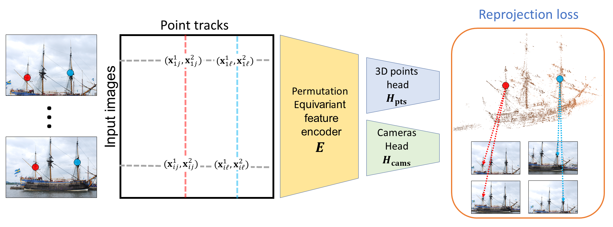
Figure 1: Overview of our method. The input is a sparse $m\times n\times 2$ tensor whose rows represent images (cameras) and columns represent point tracks. Each filled entry in the tensor specifies the 2D coordinates of a 3D point in a specific image. This tensor is processed by a permutation equivariant feature encoder that respects the data symmetries: reoredeing of the rows and the columns of the input tensor. The model outputs a set of points and a set of camera matrices using two dedicated sub-networks (heads). The model is optimized using an unsupervised reprojection loss, which minimizes the discrepancies in projecting the recovered 3D points relatively to the 2D positions of the input tracks.

Our work is inspired by both projective factorization approaches to SFM (e.g., [8, 31, 33]) and by deep matrix completion networks for, e.g., collaborative filtering applications [4, 16]. Projective factorization techniques seek to express a matrix of track positions as a function of two matrices, a matrix of camera pose parameters and a matrix of 3D point positions. Deep matrix completion methods opt to predict the missing values in an input matrix by learning a function of its unknown factors. Key to deep matrix completion architectures is their equivariant architecture; i.e., reordering the rows or columns of the input matrix should yield the same predictions, reordered accordingly. Analogously to convolutional networks for images, such an equivariant architecture is efficient, requiring fewer parameters than standard MLP alternatives, and imposes an appropriate inductive bias that promotes training with fewer samples.

Below we introduce an equivariant network architecture for SFM (see Figure 1) that enables simultaneous recovery of camera parameters and scene structure in both calibrated and uncalibrated settings. Specifically, given a tensor of track positions, possibly with many missing elements, we seek to express this tensor as a function of the unknown camera pose parameters and 3D point positions. We use an equivariant network architecture; changing the order of images (rows of the track tensor) yields the same reordering of the recovered cameras; changing the order of the point tracks (tensor columns) yields an equivalent reorder of the recovered 3D points. Our network can be applied in a single scene scenario, in which for a given scene the weights are optimized to directly minimize a reprojection loss. This minimization does not require initialization of either camera parameters or scene structure, yet it achieves accurate recovery of poses and scene structure, on par with state of the art methods.

A significant contribution of this paper is in showing that this type of architecture also enables generalization to novel scenes. Specifically, we use unsupervised learning to train our network on multiple scenes and then apply the network at inference time to novel scenes. Our experiments indicate that a short refinement step and standard bundle adjustment enables accurate prediction of camera poses and 3D point positions for novel scenes in just a few minutes for scenes including hundreds of images and hundreds of thousands of track points. We finally compare our method, in addition to state of the art baselines, also to two novel network architectures: a network based on DeepSets [68] and a graph neural network. We discuss the advantages and weaknesses of these approaches.

We believe that our method is a step forward in using the deep learning machinery for solving large and challenging SFM problems. Specifically, our method can be leveraged in the future for constructing an end-to-end model that takes a set of images and outputs the camera positions and 3D points coordinates directly without any additional pre-processing and post-processing steps. Our code and data are available at https://github.com/drormoran/Equivariant-SFM.

2 Previous work

Classical SFM methods.

Structure from motion has a long history in computer vision [32]. Advances in projective geometry and optimization [18] yielded many effective algorithms. A popular approach involves a sequential processing of the input images [51, 64, 47, 33], so that at each step one image is added, the respective camera pose is recovered, and bundle adjustment is applied to refine the accumulated poses and 3D structure. More recently global techniques based on motion averaging were proposed. Early methods first denoise the relative rotation between pairs of views, and subsequently denoise the relative translations and scales [37, 2, 6, 11, 62, 40, 23, 5, 54]. Recent works apply averaging directly to the fundamental and essential matrices [25, 26, 14, 50]. Another approach uses factorization-based methods [8, 31, 10, 28, 33, 38, 52, 55, 3]. These methods factor a tensor of point tracks into a product of unknown camera matrices, depth values, and 3D point locations. These methods typically yield very large optimization problems and are often approached by splitting the problem into smaller subproblems. Finally, Initialization-free-bundle-adjustment methods [21, 20, 19] use a variable projection method, designed to optimally eliminate subsets of the unknowns, to allow better convergence of bundle adjustment from arbitrary initializations.

Deep SFM methods.

The rise of deep neural networks has led to new, network-based algorithms for pose estimation and 3D reconstruction. Specifically, [56, 58, 69] recover camera pose for two or three input images, and a dense depth map for one image. BA-net [53] and DeepSFM [61] are intended to recover pose in multiview settings, but due to memory limitations (the algorithms rely on fine sampling of the cost volume) their method can handle only a handful of views. The latter also requires initialization of the pose parameters. IDR [67] recovers pose and dense structure (using an implicit neural representation), but it requires near accurate initialization of camera pose as well as masked images, and hence it is unsuitable for general scenes. NeuRoRA [43] introduced a graph neural network architecture for rotation averaging from noisy and incomplete set of relative pairwise orientations. However, their method does not recover camera locations. Of some relevance also is Posenet [27], which is trained to estimate absolute camera pose for a particular (trained) scene. Finally, [60] enables initialization-free camera and depth recovery for setups that involve cameras facing roughly the same direction. In contrast to these, our method is applied to general scenes with hundreds of images and no initialization. However, like classical methods it only produces a sparse reconstruction.

Learning on sets and equivariance.

Using equivariance as a design principle is a popular approach for constructing efficient neural architectures, see, for example, [9, 63, 46, 29, 12, 34]. Here, we focus on equivariant architectures for set-structured data.

Learning on set-structured data, where each data point consists of several items and the learning task is invariant or equivariant to their order, is a prominent research direction in recent years. [45, 68, 44] pioneered this area by suggesting the first universal deep architectures for this setup. [30] extended these works by incorporating attention mechanisms. More closely related to our work is [16], which considered a setup that models interaction across several sets: the input is a matrix (more generally, a tensor) and the learning task is equivariant to permutations of both its rows and its columns (and other dimensions in the general case). The paper characterized the maximally expressive linear equivariant layers for this setup and used them for constructing equivariant deep models. These models were shown to perform well in matrix completion and recommender system applications. This learning setup was later generalized to sets of arbitrary symmetric elements [36] and to hierarchical structures [59].

3 Approach

3.1 Problem definition

In structure from motion we assume a stationary scene is viewed by $m$ unknown camera matrices, $P_{1},...,P_{m}$. Each camera is represented by a $3\times 4$ matrix representing maps between projective spaces $P_{i}:\mathbb{P}^{3}\longrightarrow\mathbb{P}^{2}$. In uncalibrated settings these are general matrices, defined up to scale, while in calibrated settings these represent camera positions and orientations in the following format $P_{i}=[R_{i}|\mathbf{t}_{i}]$ with $R_{i}\in SO(3)$ representing camera orientation and $\mathbf{t}_{i}\in\mathbb{R}^{3}$ so that camera position given by $-R_{i}^{T}\mathbf{t}_{i}$. Let $\mathbf{X}$ denote a 3D scene point represented in homogeneous coordinates as $\mathbf{X}=(X^{1},X^{2},X^{3},1)^{T}\in\mathbb{P}^{3}$. Its projection onto the $i$’th image is given by $\mathbf{x}=(x^{1},x^{2},1)^{T}\propto P\mathbf{X}\in\mathbb{P}^{2}$, where the symbol ’$\propto$’ denotes equality up to scale.

As with common SFM algorithms, given images of a static scene, we address the SFM problem after feature points are detected and matched, and after outlier matches are removed by robust recovery of essential or fundamental matrices between pairs of images. The input to our algorithm includes a set of tracks $T_{1},...,T_{n}$, where each track is a set of 2D point positions, $T_{j}=\{\mathbf{x}_{ij}\}_{i\in C_{j}}$, and $C_{j}\subseteq[m]$ denotes images in which $\mathbf{X}_{j}$ is detected. The collection of tracks is arranged in a (typically sparse) measurement tensor $M$ of size $m\times n\times 2$ such that $(M_{ij1},M_{ij2},1)^{T}=\mathbf{x}_{ij}$, or these entries are empty if $\mathbf{X}_{j}$ is not detected in $I_{i}$. Given $M$, we aim to recover the camera matrices ${\cal P}=\{P_{1},...,P_{m}\}$ and the 3D positions ${\cal X}=\{\mathbf{X}_{1},\mathbf{X}_{2},...\mathbf{X}_{n}\}$ of the respective point tracks.

3.2 Model

Our main design motivation is building a model that respects the symmetries of the task above. We will now describe these symmetries, define a suitable model and discuss its advantages.

Task symmetries.

Our network takes as input a sparse $m\times n\times 2$ tensor $M$ and outputs two matrices: $P\in\mathbb{R}^{m\times 12}$ that represents the set of cameras and $X\in\mathbb{R}^{n\times 3}$ that represents a set of points. Importantly, our model should respect the order of the cameras ${\cal P}$ and the scene points ${\cal X}$ in the measurements tensor $M$. More formally, let $S_{d}$ denote the group of permutations on $d$ elements and let $\tau_{\mathrm{cams}}\in S_{m}$ and $\tau_{\mathrm{pts}}\in S_{n}$. Intuitively, we can think of these permutations as a specific ordering of the cameras and the 3D points. $S_{n}$ and $S_{m}$ act on our measurement tensor $M$ by permuting its rows and columns (Figure 2): $((\tau_{\mathrm{cams}},\tau_{\mathrm{pts}})\cdot M)_{ij}=M_{\tau_{\mathrm{cams}}^{-1}(i),\tau_{\mathrm{pts}}^{-1}(j)}$. As the order of cameras and points is arbitrary, it is natural to expect that the outputs will be reordered according to any given input order. This argument suggests that our network $F$ should follow the following transformation rule for all $\tau_{\mathrm{cams}}\in S_{m},\tau_{\mathrm{pts}}\in S_{n}$ and $M\in\mathbb{R}^{m\times n\times 2}$:

$$F((\tau_{\mathrm{cams}},\tau_{\mathrm{pts}})\cdot M)=(\tau_{\mathrm{cams}},\tau_{\mathrm{pts}})\cdot F(M).$$

Put differently, the network should be equivariant to the action of the direct product of the two groups, namely to $G=S_{m}\times S_{n}$. The action of $G$ on the output space should be understood here as $(\tau_{\mathrm{cams}},\tau_{\mathrm{pts}})\cdot P=\tau_{\mathrm{cams}}\cdot P$ and $(\tau_{\mathrm{cams}},\tau_{\mathrm{pts}})\cdot X=\tau_{\mathrm{pts}}\cdot X$, i.e., the permutations act only on a single dimension of each output matrix. Figure 2 illustrates this type of equivariance. We note that equivariance to direct products of permutation groups was first studied in [16].

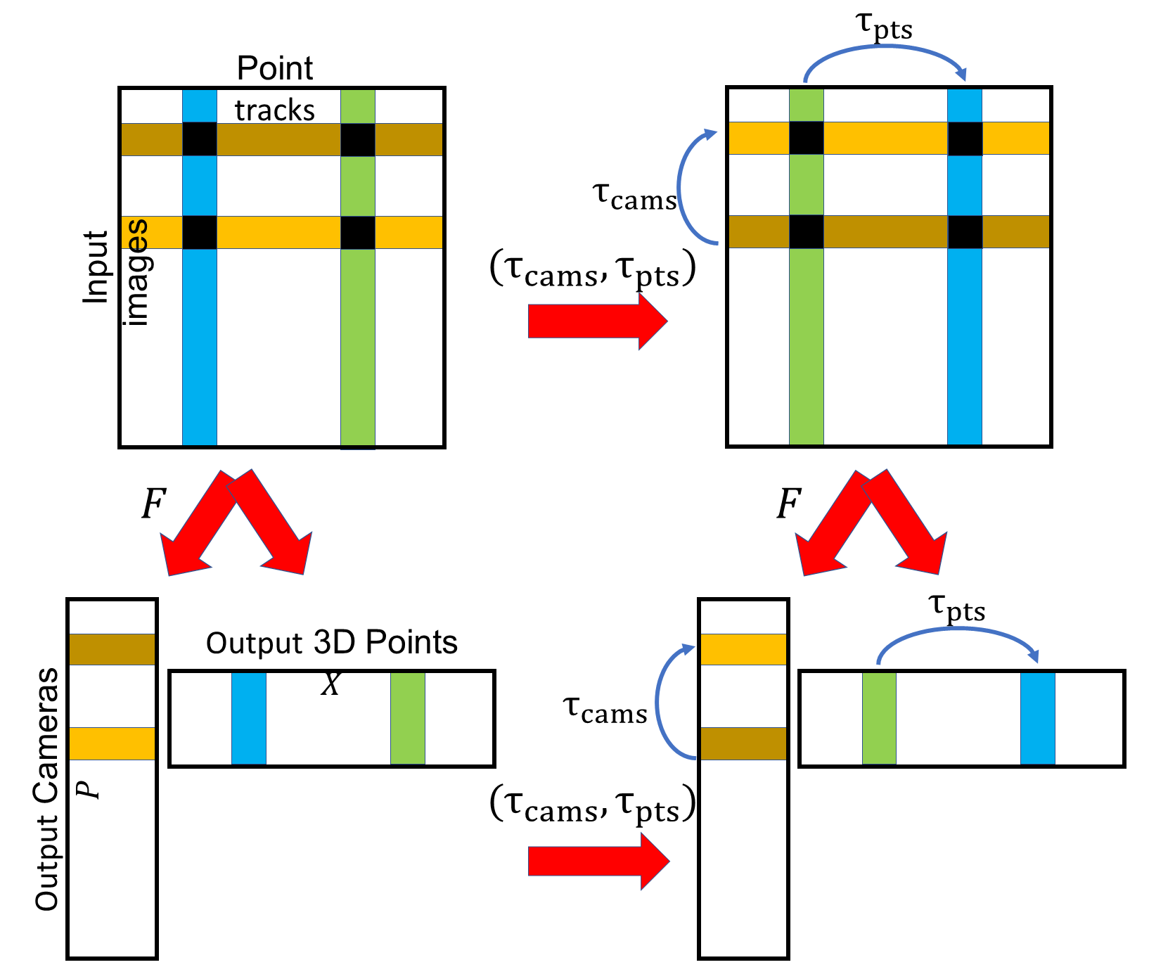
Figure 2: Predicting a set of camera positions and 3D points from an input measurement tensor $M$ is equivariant to reordering of the points and the cameras, represented by the pair of permutations $(\tau_{\mathrm{cams}},\tau_{\mathrm{pts}})$. This is illustrated in the commutative diagram above.

Equivariant Layers.

Linear equivariant maps serve as the main building blocks for equivariant networks. As shown in [16], assuming a single input and output channel, the space of linear maps that are equivariant to $G$ is 4-dimensional, and it is spanned by the identity, the row sums, the column sums, and the matrix sum. More generally, with multiple input and output channels, any $G$-equivariant affine map $L$ from a feature space with $d$ channels $\mathbb{R}^{m\times n\times d}$ to a feature space with $d^{\prime}$ channels $\mathbb{R}^{m\times n\times d^{\prime}}$ can be represented in the following way:

$$\begin{split}L(\tilde{M})_{ij}=&W_{1}\tilde{M}_{ij}+W_{2}\sum_{k=1}^{m}\tilde{M}_{kj}+\\ &W_{3}\sum_{l=1}^{n}\tilde{M}_{il}+W_{4}\sum_{k=1}^{m}\sum_{l=1}^{n}\tilde{M}_{kl}+\mathbf{b},\end{split}$$ (1)

where for the input tensor $\tilde{M}_{ij}$ is a vector in $\mathbb{R}^{d}$, $W_{i}\in\mathbb{R}^{d^{\prime}\times d}$ for $i=1,...,4$, and $\mathbf{b}\in\mathbb{R}^{d^{\prime}}$ are learnable parameters. Equivalently, $L$ can be represented as an $mnd^{\prime}\times mnd$ matrix with a parameter sharing scheme governed by (1) (see [46, 34] for the connection between equivariance and parameter sharing) and possibly an additional bias term. Here we replace sums by averages over the non-empty entries of $M$ to maintain indifference to missing data.

Network architecture.

Our network is composed of three main parts (see Figure 1): a shared feature encoder $E$ and two sub-networks (heads), $H_{\mathrm{cams}}$ and $H_{\mathrm{pts}}$, that produce the recovered cameras and 3D points from the features encoded by $E$. The shared feature encoder takes the input tensor $M\in\mathbb{R}^{m\times n\times 2}$ and outputs a latent representation $\mathbb{R}^{m\times n\times d}$ while maintaining the sparsity pattern of the input. As usually done when constructing equivariant networks [68, 16], the feature encoder is comprised of a composition of several linear equivariant layers interleaved with pointwise nonlinearities such as the ReLU function:

$$E=L_{k}\circ\sigma\circ\cdots\circ\sigma\circ L_{1},$$ (2)

where $L_{i},~{}i=1...k$, are $G$-equivariant layers as in (1) and $\sigma$ is the pointwise nonlinearity. Importantly, the pointwise nonlinearities maintain equivariance to the permutation action, implying that the complete composition is equivariant.

The first head $H_{\mathrm{cams}}$ takes as input a pooled average of the latent representation, $(1/|\bar{C}_{i}|)\sum_{j\in\bar{C}_{i}}E(M)_{i,j}\in\mathbb{R}^{m\times d}$, where $\bar{C}_{i}$ denotes the set of track points detected in image $i$, and outputs a matrix representation of the camera parameters. In the uncalibrated setting this results in a matrix $P\in\mathbb{R}^{m\times 12}$, and each row is used to populate the corresponding $3\times 4$ camera matrix $P_{i}$. In the calibrated setting this head produces an $m\times 7$ matrix, and we use the first four components in each row to construct a quaternion vector that represents the $i$’th camera orientation and the last three components to construct the camera translation vector. The second head $H_{\mathrm{pts}}$ takes as input $(1/|C_{j}|)\sum_{i\in C_{j}}E(M)_{i,j}\in\mathbb{R}^{n\times d}$, where $C_{j}$ denotes the track points corresponding to $X_{j}$, and outputs a matrix representation of the 3D points $X\in\mathbb{R}^{n\times 3}$. As the pooled versions of the latent representations used by the sub-networks result in single set structures, both heads are implemented as standard equivariant set networks (element-wise fully connected layers) [44].

Discussion.

There are several important advantages to using our equivariant architecture compared to standard fully connected architectures. Above all, our architecture encodes the structure of the task into the model, thus providing a strong inductive bias. Additional benefits include (1) considerable reduction in the number of parameters: for example, the linear part of the layer described in (1) has $4dd^{\prime}$ free parameters instead of $n^{2}m^{2}dd^{\prime}$ free parameters in a suitable fully connected architecture; (2) improved efficiency due to small matrix multiplications as seen in Equation (1); (3) better generalization: training on any input tensor exposes the network to all its different realizations by different point and camera orders; and (4) Our architecture has the crucial ability to handle variable sized inputs and varying patterns of missing entries in the input tensor. Finally, while equivariant/invariant models might suffer from loss of expressive power [65, 35], it was proven that the network architecture we use enjoys a universal approximation property (for full tensors under mild assumptions on the input domain) [36], i.e., with sufficient layers and channels and with a proper set of weights it is capable of approximating any continuous $G$-equivariant function.

3.3 Loss function

Our network minimizes a loss function made of two terms, a reprojection loss and a hinge loss. The reprojection loss, similar to bundle adjustment, minimizes the discrepancies in projecting the recovered 3D points $\mathbf{X}_{k}$ compared to their detected locations in the images (see Figure 1). Additionally, we use a hinge loss to discourage the recovered depth values from vanishing or becoming negative.

Let $\mathbf{x}_{ij}$ be a point from track $T_{j}$ detected in image $I_{i}$. Let the unknown $P_{i}$ denote the respective camera, and let $\mathbf{X}_{j}$ denote the unknown 3D position of the points in $T_{j}$. To properly measure projective depth in the uncalibrated case (see discussion in [18], Chapter 21 Cheirality) we normalize each camera matrix $P_{i}$ so that its left $3\times 3$ block has positive determinant and unit norm third row. (These conditions are fulfilled by construction in the calibrated case.)

We next let

$$r_{ij}=\left\lVert\left(\mathbf{x}_{ij}^{1}-\frac{P_{i}^{1}\mathbf{X}_{j}}{P_{i}^{3}\mathbf{X}_{j}},\mathbf{x}_{ij}^{2}-\frac{P_{i}^{2}\mathbf{X}_{j}}{P_{i}^{3}\mathbf{X}_{j}}\right)\right\rVert,$$

where $P_{i}^{k}$ denotes the $k$’th row of the camera matrix $P_{i}$. Thus, $r_{ij}$ measures the reprojection error of $\mathbf{X}_{j}$ in image $I_{i}$. Next, we define $h_{ij}=\max(0,h-P_{i}^{3}\mathbf{X}_{j})$, where $h>0$ is a small constant (in our setting, $h=0.0001$). $h_{ij}$ therefore is the hinge loss for the depth value of $\mathbf{X}_{j}$ in image $I_{i}$.

We combine $r_{ij}$ and $h_{ij}$ as follows,

$$s_{ij}=\begin{cases}r_{ij},~{}~{}&P_{i}^{3}\mathbf{X}_{j}\geq h\\ h_{ij},~{}~{}&P_{i}^{3}\mathbf{X}_{j}<h,\end{cases}$$

and finally define our loss function as

$${\cal L}(\{P_{i}\},\{\mathbf{X}_{j}\})=\frac{1}{p}\sum_{i=1}^{m}\sum_{j=1}^{n}\xi_{ij}s_{ij},$$ (3)

where $m$ denotes the number of cameras, $n$ the number of point tracks, $p=\sum_{j=1}^{n}|T_{j}|$ the number of measured projections, and $\xi_{ij}\in\{0,1\}$ is indicating whether point $\mathbf{X}_{j}$ is detected in image $I_{i}$. For each detected point $\mathbf{x}_{ij}$, therefore, the loss measures either reprojection error, if its recovered depth value exceeds the threshold $h$, or it measures the hinge loss, if the recovered depth is either negative or near zero. Note that for robustness we use in the reprojection loss the $\ell_{2}$ measure, as opposed to the standard MSE. We note that our loss function is not continuous at points in which a depth value is $h$. It is however differentiable almost everywhere with respect to the network weights.

3.4 Optimization and learning strategies

We apply our model in two setups. In a single scene setup given point tracks from a single scene we initialize the network with random weights and use back propagation to minimize the loss function (3). At the end we use triangulation to estimate the locations of the 3D points and apply bundle adjustment.

In the learning scenario we train the model with tracks from multiple scenes. At train time we minimize our loss function (3) while alternating between the input scenes. We evaluate success on a validation set and use early stopping to keep the model that reaches the best reprojection error on this set. To test the model on novel scenes, given a measurement tensor we either apply the network to the tensor to get an initial reconstruction, or, we fine tune the model by running back propagation for a predetermined number of epochs. We complete these with bundle adjustment. Inference with the network is extremely fast, taking roughly hundredths of a second on a DGX machine, therefore the total test time is dominated by the time of the optional fine tuning and the bundle adjustment.

4 Experimental setup

We tested our model on a variety of datasets in both single scene and learning scenarios and in both calibrated and uncalibrated settings.

4.1 Datasets and baselines

4.1.1 Uncalibrated setting

For this setting we used 39 scans from Olsson’s [39] and the VGG [57] datasets. The number of images in these scans vary from 10 to 400 and number of points in the track tensors from 300 to 150K. We compare our method to the following baselines.

VARPRO [21]. An initialization-free optimization strategy based on variable projection (VarPro) applied to projective bundle adjustment.

GPSFM [26]. A global algorithm based on averaging of fundamental matrices. The algorithm minimizes an algebraic loss, i.e., it seeks the nearest collection of fundamental matrices that can be realized with projective cameras.

PPSFM [33]. A sequential method based on incrementally optimizing for projective structure and cameras while incorporating constraints on the sought projective depths.

4.1.2 Calibrated setting

For this setting we used 36 scans from Olsson’s dataset [39]. The dataset includes “ground truth” camera parameters, including intrinsic and extrinsic (locations and orientations) parameters, which in fact are reconstructed with Olsson’s SFM method. The number of cameras ranges from 12 to 419 and the number of points in the track tensor from 319 to 156k.

GESFM [25]. Analogously to GPSFM, this is a global algorithm based on averaging essential matrices. The algorithm minimizes an algebraic loss, i.e., it seeks the nearest collection of essential matrices that can be realized with Euclidean cameras.

Linear [23]. This algorithm enforces the consistency of camera triplets while minimizing an approximate geometric error. (For this algorithm we were unable to find one set of threshold parameters that works on all the datasets, and so for each scan we report the best run.)

COLMAP [47, 48, 49] A state-of-the-art sequential method.

4.2 Implementation details

Framework. Our method was run on NVIDIA Quadro RTX 8000/ RTX 6000/ DGX V100 GPUs. We used PyTorch [42] as the deep learning framework, and ADAM optimizer with normalized gradients. For experiments involving graphs (Section 5.4) we use PyTorch Geometric [13].

Training. In both calibrated and uncalibrated settings we randomly divided the datasets to three parts: 10 scenes for test, 3 for validation, and the rest for training. During training we alternated between the different training scenes, where in each epoch we trained on a random subset of 10-20 images in a scene. We used validation for early stopping. Validation and test were applied to the complete scenes.

Optimization. Since dividing by $P^{3}_{i}\mathbf{X}_{j}$ can result in exploding gradients, during back-propagation we normalized the gradient of $P_{i}\mathbf{X}_{j}$ at each step.

Architecture details. The input to our method includes normalized point tracks $\mathbf{x}_{ij}$. In the calibrated setting we normalized the points using the known intrinsic parameters. In the unclibrated setting we used Hartley normalization [17]. For efficiency we designed our encoder to work with sparse matrices. The shared features encoder $E$ has 3 layers each with respectively 256 or 512 feature channels in the single scene and training setups and ReLU activation. The camera head $H_{\mathrm{cams}}$ and 3D point head $H_{\mathrm{pts}}$ each have 2 layers with 256 or 512 channels for optimization and training, respectively. After each layer in $E$ we normalize its features by subtracting their mean.

Hyper-parameter search. We tested our model with different hyper-parameters including: (1) learning rates in $\{1e-2,1e-3,1e-4\}$, (2) network width for the encoder $E$ and heads in $\{128,256,512\}$, (3) number of layers in these networks $\{2,3\}$, (4) depth threshold $h\in\{1e-2,1e-3,1e-4\}$, (5) std normalization for the layer output in (1).

Bundle adjustment For bundle adjustment we used the Ceres BA implementation [1] with the Huber loss (with parameter 0.1) for robustness and limited the number of iterations to 100.

4.3 Evaluation

In the uncalibrated setting we measure accuracy with the average reprojection error, measured in pixels as follows

$$\frac{1}{p}\sum_{i=1}^{m}\sum_{j=1}^{n}\xi_{ij}\left\lVert\left(\mathbf{x}_{ij}^{1}-\frac{P_{i}^{1}\mathbf{X}_{j}}{P_{i}^{3}\mathbf{X}_{j}},\mathbf{x}_{ij}^{2}-\frac{P_{i}^{2}\mathbf{X}_{j}}{P_{i}^{3}\mathbf{X}_{j}}\right)\right\rVert.$$

For notation see Sec. 3.3. In the calibrated case we further evaluate our predictions of the external camera parameters. Specifically, we compare our camera orientation predictions with ground truth ones by measuring their angular difference in degrees, as well as the difference between our predicted and ground truth camera locations in meters. For fair comparison, both our method and all the baseline methods were run with the same set of point tracks. For all methods we apply a final post-processing step of bundle adjustment. Below we show results both before and after BA (results before BA for the baseline methods are provided in the supplementary material).

5 Results

Scan #Images #Points Reprojection error (pixels) Ours Ours GPSFM PPSFM VarPro No BA Alcatraz Courtyard $133$ $23674$ $1.55$ $\mathbf{0.52}$ $\mathbf{0.52}$ $0.57$ $\mathbf{0.52}$ Alcatraz Water Tower $172$ $14828$ $2.18$ $\mathbf{0.47}$ $0.63$ $0.59$ $\mathbf{0.47}$ Alcatraz West Side Gardens $419$ $65072$ $9.54$ $\mathbf{0.76}$ $326.99$ $1.77$ - Basilica Di San Petronio $334$ $46035$ $7.9$ $0.96$ $60.69$ $\mathbf{0.63}$ - Buddah Statue $322$ $156356$ $18.88$ $2.93$ $96.96$ $\mathbf{0.41}$ - Buddah Tooth Relic Temple Singapore $162$ $27920$ $4.59$ $\mathbf{0.6}$ $0.62$ $0.71$ $\mathbf{0.6}$ Corridor $11$ $737$ $0.3$ $\mathbf{0.26}$ $\mathbf{0.26}$ $0.27$ $\mathbf{0.26}$ Ecole Superior De Guerre $35$ $13477$ $0.75$ $\mathbf{0.26}$ $\mathbf{0.26}$ $0.28$ $\mathbf{0.26}$ Dinosaur 319 $36$ $319$ $2.35$ $1.53$ $\mathbf{0.43}$ $0.47$ $\mathbf{0.43}$ Dinosaur 4983 $36$ $4983$ $1.96$ $0.57$ $\mathbf{0.42}$ $0.47$ $\mathbf{0.42}$ Doge Palace Venice $241$ $67107$ $3.6$ $\mathbf{0.6}$ $3.52$ $0.67$ - Eglise du dome $85$ $84792$ $1.1$ $\mathbf{0.24}$ $\mathbf{0.24}$ $0.25$ - Drinking Fountain Somewhere in Zurich $14$ $5302$ $0.33$ $\mathbf{0.28}$ $\mathbf{0.28}$ $0.31$ $\mathbf{0.28}$ East Indiaman Goteborg $179$ $25655$ $3.31$ $0.99$ $5.11$ $\mathbf{0.67}$ - Folke Filbyter $40$ $21150$ $8.87$ $8.58$ $0.82$ $\mathbf{0.33}$ $277.89$ Golden Statue Somewhere In Hong Kong $18$ $39989$ $0.35$ $\mathbf{0.22}$ $\mathbf{0.22}$ $0.24$ $\mathbf{0.22}$ Gustav Vasa $18$ $4249$ $0.23$ $\mathbf{0.16}$ $\mathbf{0.16}$ $0.17$ $\mathbf{0.16}$ GustavIIAdolf $57$ $5813$ $14.77$ $5.83$ $\mathbf{0.23}$ $0.24$ $\mathbf{0.23}$ Model House $10$ $672$ $0.37$ $\mathbf{0.34}$ $1.12$ $0.4$ $\mathbf{0.34}$ Jonas Ahlstromer $40$ $2021$ $14.38$ $4.72$ $\mathbf{0.18}$ $0.2$ $\mathbf{0.18}$ Lund University Sphinx $70$ $32668$ $3.64$ $\mathbf{0.34}$ $0.45$ $0.37$ $\mathbf{0.34}$ Nijo Castle Gate $19$ $7348$ $0.71$ $\mathbf{0.39}$ $\mathbf{0.39}$ $0.43$ $\mathbf{0.39}$ Pantheon Paris $179$ $29383$ $1.75$ $\mathbf{0.49}$ $2.85$ $0.62$ - Park Gate Clermont Ferrand $34$ $9099$ $0.61$ $\mathbf{0.31}$ $0.32$ $0.49$ $\mathbf{0.31}$ Plaza De Armas Santiago $240$ $26969$ $5.1$ $\mathbf{0.64}$ $3.14$ $0.71$ - Porta San Donato Bologna $141$ $25490$ $1.58$ $\mathbf{0.4}$ $0.61$ $3.75$ $\mathbf{0.4}$ The Pumpkin $195$ $69335$ $14.45$ $\mathbf{0.38}$ $\mathbf{0.38}$ $0.42$ - Skansen Kronan Gothenburg $131$ $28371$ $1.19$ $\mathbf{0.41}$ $0.44$ $0.44$ - Skansen Lejonet Gothenburg $368$ $74423$ $10.82$ $2.05$ $7.48$ $\mathbf{1.28}$ - Smolny Cathedral St Petersburg $131$ $51115$ $1.66$ $\mathbf{0.46}$ $\mathbf{0.46}$ $0.5$ - Some Cathedral In Barcelona $177$ $30367$ $3.67$ $\mathbf{0.51}$ $\mathbf{0.51}$ $0.54$ - Sri Mariamman Singapore $222$ $56220$ $7.06$ $\mathbf{0.61}$ $0.78$ $0.85$ - Sri Thendayuthapani Singapore $98$ $88849$ $2.12$ $\mathbf{0.31}$ $0.56$ $0.33$ - Sri Veeramakaliamman Singapore $157$ $130013$ $6.47$ $\mathbf{0.52}$ $1.78$ $0.66$ - Thian Hook Keng Temple Singapore $138$ $34288$ $7.59$ $\mathbf{0.54}$ $0.55$ $0.66$ $\mathbf{0.54}$ King’s College U. of Toronto $77$ $7087$ $2.27$ $0.78$ $2.35$ $0.26$ $\mathbf{0.24}$ Tsar Nikolai I $98$ $37857$ $6.04$ $2.43$ $0.33$ $0.31$ $\mathbf{0.29}$ Urban II $96$ $22284$ $16.91$ $6.84$ $\mathbf{0.27}$ $0.31$ $3.61$

Table 1: Single scene results with our method against baselines in the uncalibrated setup. The table shows average reprojection error before and after BA. (Smaller is better.) In a number of experiments VarPro exceeded either memory or runtime limitations. These experiments are marked by the missing entries.

Scan #Images #Points $\mathbf{t}_{\text{error}}$ $R_{\text{error}}$ Reprojection Error Ours Ours GESFM Linear Colmap Ours Ours GESFM Linear Colmap Ours Ours GESFM Linear Colmap No BA No BA No BA Alcatraz Courtyard $133$ $23674$ $0.16$ $0.015$ $0.259$ $\mathbf{0.014}$ $\mathbf{0.014}$ $0.619$ $0.049$ $0.533$ $\mathbf{0.042}$ $0.043$ $1.64$ $\mathbf{0.81}$ $4.67$ $1.27$ $\mathbf{0.81}$ Alcatraz Water Tower $172$ $14828$ $0.518$ $0.116$ $9.147$ $1.643$ $\mathbf{0.115}$ $0.933$ $0.23$ $9.997$ $1.525$ $\mathbf{0.228}$ $2.13$ $\mathbf{0.55}$ $25.93$ $73.72$ $\mathbf{0.55}$ Buddah Tooth Relic Temple Singapore $162$ $27920$ $0.233$ $\mathbf{0.014}$ $1.429$ $0.125$ $0.015$ $1.03$ $\mathbf{0.081}$ $4.709$ $0.551$ $0.083$ $2.06$ $\mathbf{0.85}$ $13.22$ $2.66$ $\mathbf{0.85}$ Doge Palace Venice $241$ $67107$ $0.342$ $0.029$ $1.608$ - $\mathbf{0.012}$ $1.163$ $0.211$ $5.317$ - $\mathbf{0.031}$ $3.62$ $1.0$ $22.32$ - $\mathbf{0.98}$ Door Lund $12$ $17650$ $0.006$ $\mathbf{0.001}$ $(0.973)$ $\mathbf{0.001}$ $\mathbf{0.001}$ $0.024$ $0.006$ $(7.552)$ $\mathbf{0.005}$ $\mathbf{0.005}$ $0.32$ $\mathbf{0.3}$ $(9.21)$ $\mathbf{0.3}$ $\mathbf{0.3}$ Drinking Fountain Somewhere In Zurich $14$ $5302$ $0.004$ $\mathbf{0.002}$ $(0.002)$ $\mathbf{0.002}$ $\mathbf{0.002}$ $0.031$ $\mathbf{0.007}$ $(0.01)$ $\mathbf{0.007}$ $\mathbf{0.007}$ $0.33$ $0.31$ $(0.27)$ $0.31$ $0.31$ East Indiaman Goteborg $179$ $25655$ $0.621$ $0.509$ $3.099$ $(2.235)$ $\mathbf{0.065}$ $3.814$ $3.117$ $12.396$ $(3.284)$ $\mathbf{0.251}$ $4.13$ $1.85$ $32.37$ $(312.9)$ $\mathbf{0.89}$ Ecole Superior De Guerre $35$ $13477$ $0.081$ $0.005$ $(0.002)$ $0.005$ $0.005$ $0.318$ $\mathbf{0.024}$ $(0.035)$ $\mathbf{0.024}$ $\mathbf{0.024}$ $0.72$ $0.34$ $(0.14)$ $0.34$ $0.34$ Eglise du dome $85$ $84792$ $0.205$ $\mathbf{0.01}$ $(1.425)$ $0.046$ $\mathbf{0.01}$ $0.808$ $0.037$ $(3.631)$ $0.162$ $\mathbf{0.036}$ $0.91$ $\mathbf{0.27}$ $(6.21)$ $0.76$ $\mathbf{0.27}$ Folke Filbyter $40$ $21150$ $0.125$ $0.118$ $(0.0)$ $0.123$ $\mathbf{0.0}$ $74.596$ $70.157$ $(0.148)$ $4.484$ $\mathbf{0.036}$ $10.37$ $4.29$ $(0.41)$ $6.06$ $\mathbf{0.29}$ Fort Channing Gate Singapore $27$ $23627$ $0.093$ $\mathbf{0.008}$ $\mathbf{0.008}$ $0.013$ $\mathbf{0.008}$ $0.207$ $\mathbf{0.02}$ $\mathbf{0.02}$ $0.029$ $\mathbf{0.02}$ $0.52$ $\mathbf{0.25}$ $\mathbf{0.25}$ $0.45$ $\mathbf{0.25}$ Golden Statue Somewhere In Hong Kong $18$ $39989$ $0.073$ $\mathbf{0.004}$ $\mathbf{0.004}$ $\mathbf{0.004}$ $\mathbf{0.004}$ $0.292$ $0.031$ $0.03$ $\mathbf{0.022}$ $0.031$ $0.4$ $\mathbf{0.27}$ $\mathbf{0.27}$ $0.3$ $\mathbf{0.27}$ Gustav Vasa $18$ $4249$ $1.085$ $1.145$ $(0.101)$ $\mathbf{0.099}$ $0.1$ $34.181$ $32.266$ $(0.751)$ $0.839$ $0.841$ $3.52$ $3.15$ $(0.31)$ $0.48$ $0.48$ GustavIIAdolf $57$ $5813$ $9.714$ $8.524$ $\mathbf{0.004}$ $\mathbf{0.004}$ $\mathbf{0.004}$ $67.784$ $58.458$ $\mathbf{0.021}$ $\mathbf{0.021}$ $\mathbf{0.021}$ $13.91$ $11.49$ $\mathbf{0.26}$ $\mathbf{0.26}$ $\mathbf{0.26}$ Jonas Ahlstromer $40$ $2021$ $10.888$ $10.451$ $(0.01)$ $1.259$ $0.011$ $50.19$ $47.117$ $(0.082)$ $5.391$ $\mathbf{0.036}$ $10.82$ $8.41$ $(0.69)$ $4.69$ $\mathbf{0.22}$ King’s College University Of Toronto $77$ $7087$ $0.235$ $0.017$ $(0.005)$ $(1.877)$ $0.017$ $0.989$ $0.085$ $(0.059)$ $(4.624)$ $0.084$ $0.9$ $\mathbf{0.34}$ $(0.35)$ $(7.12)$ $\mathbf{0.34}$ Lund University Sphinx $70$ $32668$ $4.585$ $2.191$ $0.016$ $1.512$ $\mathbf{0.009}$ $19.522$ $8.752$ $0.058$ $5.452$ $\mathbf{0.033}$ $4.78$ $1.36$ $0.4$ $4.58$ $\mathbf{0.39}$ Nijo Castle Gate $19$ $7348$ $0.286$ $0.012$ $\mathbf{0.011}$ $0.19$ $\mathbf{0.011}$ $1.495$ $0.069$ $\mathbf{0.064}$ $0.744$ $\mathbf{0.064}$ $1.7$ $\mathbf{0.73}$ $\mathbf{0.73}$ $4.84$ $\mathbf{0.73}$ Pantheon Paris $179$ $29383$ $0.05$ $\mathbf{0.005}$ $0.595$ $0.011$ - $0.192$ $\mathbf{0.04}$ $3.208$ $0.072$ - $1.47$ $\mathbf{0.49}$ $9.71$ $0.82$ - Park Gate Clermont Ferrand $34$ $9099$ $0.125$ $\mathbf{0.022}$ $\mathbf{0.022}$ $\mathbf{0.022}$ $\mathbf{0.022}$ $0.391$ $\mathbf{0.049}$ $\mathbf{0.049}$ $\mathbf{0.049}$ $\mathbf{0.049}$ $0.57$ $\mathbf{0.35}$ $\mathbf{0.35}$ $\mathbf{0.35}$ $\mathbf{0.35}$ Plaza De Armas Santiago $240$ $26969$ $2.944$ $1.383$ $2.244$ - $\mathbf{0.048}$ $6.782$ $2.556$ $6.344$ - $\mathbf{0.122}$ $7.4$ $4.9$ $15.61$ - $\mathbf{1.13}$ Porta San Donato Bologna $141$ $25490$ $0.388$ $\mathbf{0.046}$ $0.169$ $0.067$ $0.047$ $2.153$ $\mathbf{0.095}$ $0.513$ $0.149$ $0.099$ $2.28$ $\mathbf{0.75}$ $3.23$ $1.16$ $\mathbf{0.75}$ Round Church Cambridge $92$ $84643$ $1.003$ $0.582$ $0.493$ $\mathbf{0.012}$ $\mathbf{0.012}$ $2.451$ $1.107$ $1.851$ $\mathbf{0.033}$ $0.035$ $2.66$ $1.54$ $2.03$ $0.41$ $\mathbf{0.39}$ Skansen Kronan Gothenburg $131$ $28371$ $0.226$ $0.008$ $0.008$ $(0.007)$ $0.008$ $0.736$ $0.026$ $0.025$ $(0.02)$ $0.025$ $1.24$ $\mathbf{0.67}$ $\mathbf{0.67}$ $(0.69)$ $\mathbf{0.67}$ Smolny Cathedral St Petersburg $131$ $51115$ $0.051$ $\mathbf{0.006}$ $0.007$ - $\mathbf{0.006}$ $0.554$ $0.033$ $\mathbf{0.028}$ - $0.029$ $1.66$ $\mathbf{0.81}$ $1.0$ - $\mathbf{0.81}$ Some Cathedral In Barcelona $177$ $30367$ $0.315$ $0.011$ $0.013$ $0.024$ $\mathbf{0.01}$ $0.88$ $0.026$ $0.031$ $0.057$ $\mathbf{0.025}$ $2.87$ $\mathbf{0.89}$ $1.09$ $2.09$ $\mathbf{0.89}$ Sri Mariamman Singapore $222$ $56220$ $0.683$ $\mathbf{0.023}$ $0.614$ $0.025$ $\mathbf{0.023}$ $2.302$ $\mathbf{0.077}$ $2.158$ $0.083$ $0.078$ $4.13$ $0.91$ $7.4$ $1.17$ $\mathbf{0.89}$ Sri Thendayuthapani Singapore $98$ $88849$ $3.812$ $2.87$ $(0.053)$ $\mathbf{0.034}$ $\mathbf{0.034}$ $46.269$ $44.17$ $(0.329)$ $\mathbf{0.138}$ $\mathbf{0.138}$ $23.37$ $8.44$ $(0.56)$ $0.72$ $0.67$ Sri Veeramakaliamman Singapore $157$ $130013$ $0.597$ $0.04$ $(1.388)$ $0.095$ $\mathbf{0.038}$ $2.559$ $0.175$ $(3.41)$ $0.288$ $\mathbf{0.169}$ $3.47$ $0.73$ $(34.72)$ $2.2$ $\mathbf{0.71}$ Statue Of Liberty $134$ $49250$ $20.012$ $4.122$ $(4.782)$ $28.049$ $\mathbf{0.099}$ $46.887$ $9.091$ $(8.281)$ $2.945$ $\mathbf{0.213}$ $26.16$ $6.97$ $(52.05)$ $5.08$ $\mathbf{1.25}$ The Pumpkin $196$ $69341$ $14.89$ $14.952$ $\mathbf{0.022}$ $(14.862)$ $\mathbf{0.022}$ $94.672$ $98.862$ $0.092$ $(3.123)$ $\mathbf{0.091}$ $33.41$ $24.85$ $\mathbf{0.57}$ $(24.19)$ $\mathbf{0.57}$ Thian Hook Keng Temple Singapore $138$ $34288$ $0.082$ $\mathbf{0.008}$ $0.024$ $0.043$ $\mathbf{0.008}$ $0.832$ $\mathbf{0.081}$ $0.245$ $0.424$ $0.084$ $2.75$ $1.13$ $3.32$ $4.92$ $\mathbf{1.12}$ Tsar Nikolai I $98$ $37857$ $9.467$ $7.836$ $\mathbf{0.005}$ $\mathbf{0.005}$ $\mathbf{0.005}$ $48.499$ $36.28$ $\mathbf{0.018}$ $\mathbf{0.018}$ $\mathbf{0.018}$ $9.79$ $6.53$ $\mathbf{0.33}$ $\mathbf{0.33}$ $\mathbf{0.33}$ Urban II $96$ $22284$ $9.467$ $9.586$ $0.036$ $3.038$ $\mathbf{0.021}$ $47.49$ $48.214$ $0.175$ $16.348$ $\mathbf{0.107}$ $9.38$ $6.92$ $0.72$ $17.61$ $\mathbf{0.38}$ Vercingetorix $69$ $10754$ $8.788$ $3.104$ $0.3$ $1.564$ $\mathbf{0.011}$ $69.328$ $17.706$ $1.431$ $7.138$ $\mathbf{0.048}$ $5.08$ $1.5$ $0.54$ $2.93$ $\mathbf{0.23}$ Yueh Hai Ching Temple Singapore $43$ $13774$ $0.098$ $\mathbf{0.014}$ $(0.023)$ $0.059$ $\mathbf{0.014}$ $0.72$ $\mathbf{0.043}$ $(0.075)$ $0.26$ $\mathbf{0.043}$ $0.94$ $\mathbf{0.65}$ $(1.64)$ $2.06$ $\mathbf{0.65}$

Table 2: Single scene results with our method before and after bundle adjustment against baselines in the calibrated setup. The table shows mean camera location error (denoted $\mathbf{t}_{\mathrm{error}}$) in meters, mean orientation error (denoted $R_{\mathrm{error}}$) in degrees, and mean reprojection error in pixels. (Smaller is better.) In parenthesis experiments in which at least 10% of the cameras are removed.

We next present the results of our experiments. We show results in the single scene recovery and learning from multiple scenes setups. We then present an ablation study and a comparison to alternative novel neural architectures.

5.1 Single scene recovery

Tables 1 and 2 respectively show results in the uncalibrated and calibrated settings. In the majority of the cases our method achieves sub-pixel accuracies, on par with classical state of the art methods such as VarPro and Colmap. Notably, as we show in the supplementary material, already before BA our method often achieves sub-pixel accuracies, significantly surpassing GPSFM. We also note that unlike the baseline methods, which often remove a subset of the cameras (we marked experiments in which at least 10% of the cameras are removed with parenthesis), our results are evaluated on all cameras. However, in a few cases our method did not converge to a favorable solution. We observe in these cases that the network reached a minimum in which a subset of the cameras are close to their ground truth positions, while the others appear to be displaced by a different global transformation. This could be resolved using sequential optimization, see supplementary material for more details and results. We note that our comparison to VarPro is partial, since in a number of experiments it exceeded either memory or runtime limitations.

5.2 Learning from multiple scenes

Scan #Images #Points Reprojection error (pixels) Inference Fine tuning Opt. (short) VarPro Alcatraz Water Tower 172 14828 $7.37$ $\mathbf{0.47}$ $6.46$ $\mathbf{0.47}$ Dinosaur 319 36 319 $1.58$ $1.30$ $1.71$ $\mathbf{0.43}$ Dinosaur 4983 36 4983 $3.99$ $1.14$ $4.26$ $\mathbf{0.42}$ Eglise du dome 85 84792 $2.1$ $\mathbf{1.27}$ $3.77$ - Drinking Fountain Somewhere in Zurich 14 5302 $14.39$ $\mathbf{0.28}$ $29.9$ $\mathbf{0.28}$ Gustav Vasa 18 4249 $6.3$ $\mathbf{0.16}$ $\mathbf{0.16}$ $\mathbf{0.16}$ Nijo Castle Gate 19 7348 $3.27$ $\mathbf{0.39}$ $28.68$ $\mathbf{0.39}$ Skansen Kronan Gothenburg 131 28371 $1.64$ $\mathbf{0.41}$ $0.52$ - Some Cathedral in Barcelona 177 30367 $14.87$ $\mathbf{0.51}$ $19.79$ - Sri Veeramakaliamman Singapore 157 130013 $18.25$ $\mathbf{5.45}$ $6.95$ -

Table 3: Reprojection errors obtained by applying our trained model to test data in the uncalibrated setup. Accuracies are shown after inference and fine tuning, compared to optimization with the same number of epochs starting with random initialization as well as results with VarPro. (Smaller is better.)

Scan #Images #Points Reprojection error (pixels) Inference Fine tuning Opt. (short) Colmap Alcatraz Courtyard 133 23674 $0.82$ $\mathbf{0.81}$ $1.61$ $\mathbf{0.81}$ Alcatraz Water Tower 172 14828 $\mathbf{0.55}$ $\mathbf{0.55}$ $4.6$ $\mathbf{0.55}$ Drinking Fountain Somewhere In Zurich 14 5302 $7.21$ $\mathbf{0.31}$ $110.85$ $\mathbf{0.31}$ Nijo Castle Gate 19 7348 $5.81$ $\mathbf{0.73}$ $19.0$ $\mathbf{0.73}$ Porta San Donato Bologna 141 25490 $1.1$ $0.79$ $83.02$ $\mathbf{0.75}$ Round Church Cambridge 92 84643 $0.5$ $1.51$ $28.17$ $\mathbf{0.39}$ Smolny Cathedral St Petersburg 131 51115 $15.15$ $\mathbf{0.81}$ $2.86$ $\mathbf{0.81}$ Some Cathedral In Barcelona 177 30367 $21.46$ $\mathbf{0.89}$ $1.06$ $\mathbf{0.89}$ Sri Veeramakaliamman Singapore 157 130013 $16.92$ $17.26$ $90.41$ $\mathbf{0.71}$ Yueh Hai Ching Temple Singapore 43 13774 $1.16$ $\mathbf{0.65}$ $37.31$ $\mathbf{0.65}$

Table 4: Reprojection errors obtained by applying our trained model to test data in the calibrated setup. Accuracies are shown after inference and fine tuning, compared to optimization with the same number of epochs starting with random initialization as well as results with Colmap. (Smaller is better.)

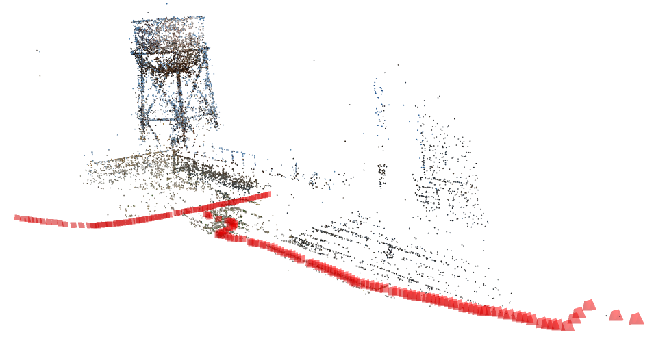
Figure 3: Recovery of 3D point clouds and camera poses in the calibrated setup obtained with our learning scheme, including inference, fine tuning and BA. Left: Alcatraz Water Tower. Right: Round Church Cambridge. Points are colored according to image intensity (darkened for better visibility) and cameras are colored in red.

Tables 4 and 4 respectively show results of testing with our trained model in both calibrated and uncalibrated settings. In each case we report reprojection error in pixels. For our method we show results both after inference with our model and after additional 500 epochs fine tuning (+ BA in both cases). These are compared to 500 epochs single scene optimization (starting with random initialization) and to state of the art VarPro and Colmap. It can be seen that with the additional fine tuning in the majority of cases our network reached sub-pixel accuracy, often on par with state of the art methods. Figure 3 shows several reconstruction results for test data.

We note that inference with our model typically takes only small fractions of a second and so the total runtime is dominated by the fine tuning and BA. For example, for the Some Cathedral In Barcelona dataset (with 177 cameras and $\sim$30K points) inference consumes only 0.007 seconds. 500 epoch fine tuning + BA take 263 seconds on a DGX machine, somewhat faster than Colmap (451s on an 8 thread, 2.2GHz CPUs), and significantly faster than our full, single scene optimization, which for this dataset with 70K epochs consumed nearly 3 hours. Run times for all tested datasets are reported in the supplementary material.

5.3 Ablation study

We have further conducted an ablation study. We tested our single scene method (a) as a simple elementwise feature encoder, i.e., with $W_{2},W_{3}$ and $W_{4}$ removed from (1), (b) directly optimizing (3) with the Adam optimizer with cameras and 3D points treated as free variables (i.e., no network), and (c) standard bundle adjustment with random initialization. Table 5 shows results in the uncalibrated setup. The results emphasize the importance of the global features, produced by $W_{2},W_{3}$ and $W_{4}$. Also, perhaps surprisingly, the Adam optimizer alone with our loss (3) achieves a significant improvement over standard bundle adjustment.

Scan Error (pixels) Ours Elementwise No BA Set Graph network network only network network Alcatraz Courtyard $\mathbf{0.52}$ $\mathbf{0.52}$ $1.31$ $191.42$ $\mathbf{0.52}$ $\mathbf{0.52}$ The Pumpkin $\mathbf{0.38}$ $6.82$ $18.67$ $324.2$ $\mathbf{0.38}$ $\mathbf{0.38}$ Alcatraz Water Tower $\mathbf{0.47}$ $\mathbf{0.47}$ $1.73$ $54.03$ $1.56$ $0.68$ Folke Filbyter $\mathbf{8.58}$ $22.8$ $35.41$ $325.62$ $30.19$ $92.24$ Gustav Vasa $\mathbf{0.16}$ $\mathbf{0.16}$ $9.06$ $34.47$ $69.11$ $\mathbf{0.16}$ Dinosaur 319 $1.53$ $1.46$ $1.29$ $13.43$ $\mathbf{0.59}$ - Park Gate Clermont Ferrand $\mathbf{0.31}$ $\mathbf{0.31}$ $\mathbf{0.31}$ $60.13$ $\mathbf{0.31}$ $\mathbf{0.31}$ Skansen Kronan Gothenburg $\mathbf{0.41}$ $1.04$ $\mathbf{0.41}$ $236.75$ $\mathbf{0.41}$ $2.08$ Smolny Cathedral St Petersburg $\mathbf{0.46}$ $\mathbf{0.46}$ $3.9$ $179.58$ $\mathbf{0.46}$ $\mathbf{0.46}$ Sri Thendayuthapani Singapore $\mathbf{0.31}$ $8.85$ $0.42$ $222.95$ $\mathbf{0.31}$ $\mathbf{0.31}$ King’s College University Of Toronto $0.78$ $0.86$ $17.02$ $36.8$ $1.07$ $\mathbf{0.63}$ Model House $\mathbf{0.34}$ $\mathbf{0.34}$ $0.92$ $26.23$ $0.52$ $\mathbf{0.34}$ Ecole Superior De Guerre $\mathbf{0.26}$ $1.83$ $\mathbf{0.26}$ $134.41$ $\mathbf{0.26}$ $\mathbf{0.26}$ Golden Statue Somewhere In Hong Kong $\mathbf{0.22}$ $0.86$ $0.89$ $24.81$ $\mathbf{0.22}$ $\mathbf{0.22}$ Dinosaur 4983 $\mathbf{0.57}$ $0.92$ $1.08$ $16.86$ $0.87$ $0.84$ Tsar Nikolai I $\mathbf{2.43}$ $5.88$ $22.09$ $99.73$ $7.4$ $2.47$ Buddah Tooth Relic Temple Singapore $\mathbf{0.6}$ $3.69$ $4.68$ $256.71$ $\mathbf{0.6}$ $\mathbf{0.6}$ Drinking Fountain Somewhere In Zurich $\mathbf{0.28}$ $\mathbf{0.28}$ $1.41$ $35.01$ $\mathbf{0.28}$ $\mathbf{0.28}$ Jonas Ahlstromer $4.72$ $\mathbf{3.8}$ $19.8$ $72.63$ $4.31$ $5.16$ Porta San Donato Bologna $\mathbf{0.4}$ $1.92$ $19.22$ $135.2$ $\mathbf{0.4}$ $\mathbf{0.4}$ Nijo Castle Gate $\mathbf{0.39}$ $\mathbf{0.39}$ $0.57$ $114.39$ $\mathbf{0.39}$ $\mathbf{0.39}$ Corridor $\mathbf{0.26}$ $\mathbf{0.26}$ $0.39$ $7.99$ $\mathbf{0.26}$ $\mathbf{0.26}$ Eglise du dome $\mathbf{0.24}$ $1.2$ $0.9$ $61.92$ $\mathbf{0.24}$ $\mathbf{0.24}$ Doge Palace Venice $\mathbf{0.6}$ $5.36$ $20.33$ $378.06$ $\mathbf{0.6}$ $0.73$ East Indiaman Goteborg $\mathbf{0.99}$ $2.33$ $21.79$ $67.96$ $2.6$ $1.13$ GustavIIAdolf $5.83$ $5.51$ $\mathbf{0.23}$ $74.63$ $5.32$ $5.28$ Lund University Sphinx $\mathbf{0.34}$ $1.74$ $12.24$ $77.69$ $0.77$ $4.62$ Pantheon Paris $\mathbf{0.49}$ $0.53$ $31.08$ $152.99$ $\mathbf{0.49}$ $\mathbf{0.49}$ Plaza De Armas Santiago $\mathbf{0.64}$ $2.36$ $2.41$ $212.0$ $\mathbf{0.64}$ $3.55$ Some Cathedral In Barcelona $\mathbf{0.51}$ $0.54$ $8.13$ $265.96$ $2.27$ $\mathbf{0.51}$ Sri Mariamman Singapore $\mathbf{0.61}$ $6.83$ $35.09$ $274.74$ $\mathbf{0.61}$ $0.62$ Sri Veeramakaliamman Singapore $\mathbf{0.52}$ $2.04$ $17.39$ $445.98$ $3.06$ $2.66$ Thian Hook Keng Temple Singapore $\mathbf{0.54}$ $0.83$ $7.45$ $405.92$ $\mathbf{0.54}$ $\mathbf{0.54}$ Urban II $6.84$ $\mathbf{6.39}$ $22.95$ $117.47$ $31.64$ $141.92$ Alcatraz West Side Gardens $\mathbf{0.76}$ $7.54$ $8.05$ $303.1$ $0.86$ $5.81$ Skansen Lejonet Gothenburg $\mathbf{2.05}$ $14.5$ $18.54$ $268.78$ $2.32$ $3.33$ Basilica Di San Petronio $0.96$ $2.99$ $27.87$ $241.3$ $1.26$ $\mathbf{0.85}$ Buddah Statue $\mathbf{2.93}$ $7.85$ $11.18$ $186.99$ $5.15$ $6.31$ Geo. Mean Ratio $1.0$ $2.35$ $5.95$ $150.8$ $1.36$ $1.52$

Table 5: Ablation Study, uncalibrated setting: reprojection errors with different components removed (see text) and with alternative network models. The last row shows for each condition the geometric mean of the ratios of reprojection errors and the corresponding errors of the full method. (Smaller is better.)

5.4 Comparison to alternative deep architectures

We have further compared our method to two novel deep architectures for SFM. The first architecture uses a set neural network [68] akin to our camera head $H_{\mathrm{cams}}$ to which we add a global feature. This network optimizes the same loss (3) with the 3D point locations treated as free variables. This network can be seen as a simpler version of our method. A second method further adds pairwise relations between the cameras, inducing a viewing graph. The input to this network further includes fundamental matrices, which are computed from the point tracks. We use a standard graph neural network [15] to optimize the loss (3). More details about these algorithms are provided in the supplementary material.

Results with these models are shown in the right two columns of Table 5. Both methods were inferior to our proposed approach, with the set network performing somewhat better than the graph network. Interestingly, simplifying our method by treating the 3D points as free variable hurts performance, and injecting the fundamental matrices to the network does not improve performance. We finally note in addition that both of these methods do not support learning.

6 Conclusion

We have introduced a novel deep-based method for multiview SFM, in both the calibrated and unclibrated settings. Starting with a (sparse) measurement tensor of point tracks, our method minimizes the reprojection loss to yield a simultaneous recovery of both camera parameters and a sparse 3D reconstruction. Importantly, we use an equivariant network architecture that respects the symmetries of the task, i.e., equivariant to permutation of either the rows (cameras) or the columns (3D points) of the measurement tensor. We have tested our method in two setups, single-scene optimization and inference with a trained model. Our experiments indicate that our method can achieve accurate pose and structure recovery, on par with classical, state-of-the-art techniques. In future work, we plan to extend this work to allow direct, end-to-end recovery from raw images and to produce dense 3D reconstruction.

Appendix

Below we provide implementation details for the baseline methods and the alternative deep architectures tested in our paper. We further include additional results, including examples of reconstructions with our method.

Appendix A Baselines

Colmap baseline.

In the calibrated experiments (Table 2 in the paper), for fair comparison, we applied Colmap [47] directly to the points tracks provided by Olsson’s dataset [39] and fixed the intrinsic camera parameters to those provided as ground truth.

Linear baseline.

We tested Jiang et al.’s method [23] while ignoring viewing graph edges for which the number of matching points was lower than a certain threshold. We used thresholds of 30, 200, 500 matching points and report those results for which the lowest reprojection error, before bundle adjustment, was obtained.

Appendix B Alternative deep architectures

The two right most columns in Table 5 in the paper show results of two novel deep architectures which were developed for comparison to our deep network architecture. The details are given below.

Set neural network.

For a scene with $m$ cameras, the input to this network is a set of $m$ random feature vectors of size 12 that provide unique ids to each camera. Inspired by [44, 68], our set network is composed of three sub-networks where each sub-network is an equivariant set network. The first sub-network is applied to each feature vector and calculates a local feature for each camera. The second sub-network is applied to each such local feature. The outputs for all cameras are then averaged, producing a global scene feature vector. Finally, the camera parameters are predicted by applying the third sub-network to both the local and global feature. In summary, the set network prediction for camera $i$ is defined as follows

$$\mathbf{z}_{i} = S_{1}(\mathbf{v}_{i})$$

$$\mathbf{z}_{g} = \frac{1}{m}\sum_{i=1}^{m}{S_{2}(\mathbf{z}_{i})}$$

$$P_{i} = S_{3}(\mathbf{z}_{i},\mathbf{z}_{g}).$$

Each $S_{k}$ is a fully connected network and $v_{i}$ is the initial random vector of camera $i$.

Graph neural network.

Here, the cameras are represented by the nodes of a graph, called the viewing graph. An edge connects a pair of nodes if the respective images share at least 30 tracks, in which case a fundamental matrix is computed. The fundamental matrices are used as edge input features, while as with the set network model, random vectors form the node input features. We use a message-passing scheme [15] and global feature as described for the set network model. Each message-passing layer is of the following form

$$\mathbf{z}_{i}^{l}=\frac{1}{|N_{i}|}\sum_{j\in N_{i}}{\mathrm{mlp}}_{l}(\mathbf{z}_{i}^{l-1},\mathbf{z}_{j}^{l-1},F_{ij})$$

where $\mathbf{z}_{i}^{l}$ is the local feature of node $i$ in layer $l$, $N_{i}$ are the neighbors of node $i$ and $F_{ij}$ is the fundamental matrix measured between cameras $i$ and $j$.

Both the set and the graph models predict camera parameters, while the 3D points are treated as free variables. In both cases we minimize the reprojection loss defined in equation (3) in the paper.

Appendix C Results

Scan #Images #Points Error (pixels) Before BA After BA Ours GPSFM Ours GPSFM PPSFM VarPro Alcatraz Courtyard $133$ $23674$ $\mathbf{1.55}$ $20.34$ $\mathbf{0.52}$ $\mathbf{0.52}$ $0.57$ $\mathbf{0.52}$ Alcatraz Water Tower $172$ $14828$ $\mathbf{2.18}$ $16.5$ $\mathbf{0.47}$ $0.63$ $0.59$ $\mathbf{0.47}$ Alcatraz West Side Gardens $419$ $65072$ $\mathbf{9.54}$ $1007.5$ $\mathbf{0.76}$ $326.99$ $1.77$ - Basilica Di San Petronio $334$ $46035$ $\mathbf{7.9}$ $1871.41$ $0.96$ $60.69$ $\mathbf{0.63}$ - Buddah Statue $322$ $156356$ $\mathbf{18.88}$ $919.26$ $2.93$ $96.96$ $\mathbf{0.41}$ - Buddah Tooth Relic Temple Singapore $162$ $27920$ $\mathbf{4.59}$ $18.53$ $\mathbf{0.6}$ $0.62$ $0.71$ $\mathbf{0.6}$ Corridor $11$ $737$ $\mathbf{0.3}$ $0.64$ $\mathbf{0.26}$ $\mathbf{0.26}$ $0.27$ $\mathbf{0.26}$ Ecole Superior De Guerre $35$ $13477$ $\mathbf{0.75}$ $1.88$ $\mathbf{0.26}$ $\mathbf{0.26}$ $0.28$ $\mathbf{0.26}$ Dinosaur 319 $36$ $319$ $\mathbf{2.35}$ $4.66$ $1.53$ $\mathbf{0.43}$ $0.47$ $\mathbf{0.43}$ Dinosaur 4983 $36$ $4983$ $1.96$ $\mathbf{1.54}$ $0.57$ $\mathbf{0.42}$ $0.47$ $\mathbf{0.42}$ Doge Palace Venice $241$ $67107$ $\mathbf{3.6}$ $170.93$ $\mathbf{0.6}$ $3.52$ $0.67$ - Eglise du dome $85$ $84792$ $\mathbf{1.1}$ $8.41$ $\mathbf{0.24}$ $\mathbf{0.24}$ $0.25$ - Drinking Fountain Somewhere In Zurich $14$ $5302$ $\mathbf{0.33}$ $1.29$ $\mathbf{0.28}$ $\mathbf{0.28}$ $0.31$ $\mathbf{0.28}$ East Indiaman Goteborg $179$ $25655$ $\mathbf{3.31}$ $99.38$ $0.99$ $5.11$ $\mathbf{0.67}$ - Folke Filbyter $40$ $21150$ $8.87$ $\mathbf{1.78}$ $8.58$ $0.82$ $\mathbf{0.33}$ $277.89$ Golden Statue Somewhere In Hong Kong $18$ $39989$ $\mathbf{0.35}$ $0.81$ $\mathbf{0.22}$ $\mathbf{0.22}$ $0.24$ $\mathbf{0.22}$ Gustav Vasa $18$ $4249$ $\mathbf{0.23}$ $1.82$ $\mathbf{0.16}$ $\mathbf{0.16}$ $0.17$ $\mathbf{0.16}$ GustavIIAdolf $57$ $5813$ $14.77$ $\mathbf{5.91}$ $5.83$ $\mathbf{0.23}$ $0.24$ $\mathbf{0.23}$ Model House $10$ $672$ $\mathbf{0.37}$ $3.66$ $\mathbf{0.34}$ $1.12$ $0.4$ $\mathbf{0.34}$ Jonas Ahlstromer $40$ $2021$ $\mathbf{14.38}$ $28.83$ $4.72$ $\mathbf{0.18}$ $0.2$ $\mathbf{0.18}$ Lund University Sphinx $70$ $32668$ $\mathbf{3.64}$ $10.0$ $\mathbf{0.34}$ $0.45$ $0.37$ $\mathbf{0.34}$ Nijo Castle Gate $19$ $7348$ $\mathbf{0.71}$ $20.08$ $\mathbf{0.39}$ $\mathbf{0.39}$ $0.43$ $\mathbf{0.39}$ Pantheon Paris $179$ $29383$ $\mathbf{1.75}$ $44.85$ $\mathbf{0.49}$ $2.85$ $0.62$ - Park Gate Clermont Ferrand $34$ $9099$ $\mathbf{0.61}$ $13.82$ $\mathbf{0.31}$ $0.32$ $0.49$ $\mathbf{0.31}$ Plaza De Armas Santiago $240$ $26969$ $\mathbf{5.1}$ $81.01$ $\mathbf{0.64}$ $3.14$ $0.71$ - Porta San Donato Bologna $141$ $25490$ $\mathbf{1.58}$ $33.36$ $\mathbf{0.4}$ $0.61$ $3.75$ $\mathbf{0.4}$ The Pumpkin $195$ $69335$ $14.45$ $\mathbf{8.97}$ $\mathbf{0.38}$ $\mathbf{0.38}$ $0.42$ - Skansen Kronan Gothenburg $131$ $28371$ $\mathbf{1.19}$ $8.9$ $\mathbf{0.41}$ $0.44$ $0.44$ - Skansen Lejonet Gothenburg $368$ $74423$ $\mathbf{10.82}$ $69.81$ $2.05$ $7.48$ $\mathbf{1.28}$ - Smolny Cathedral St Petersburg $131$ $51115$ $\mathbf{1.66}$ $83.78$ $\mathbf{0.46}$ $\mathbf{0.46}$ $0.5$ - Some Cathedral In Barcelona $177$ $30367$ $\mathbf{3.67}$ $14.77$ $\mathbf{0.51}$ $\mathbf{0.51}$ $0.54$ - Sri Mariamman Singapore $222$ $56220$ $\mathbf{7.06}$ $39.89$ $\mathbf{0.61}$ $0.78$ $0.85$ - Sri Thendayuthapani Singapore $98$ $88849$ $\mathbf{2.12}$ $13.25$ $\mathbf{0.31}$ $0.56$ $0.33$ - Sri Veeramakaliamman Singapore $157$ $130013$ $\mathbf{6.47}$ $99.99$ $\mathbf{0.52}$ $1.78$ $0.66$ - Thian Hook Keng Temple Singapore $138$ $34288$ $\mathbf{7.59}$ $26.78$ $\mathbf{0.54}$ $0.55$ $0.66$ $\mathbf{0.54}$ King’s College University Of Toronto $77$ $7087$ $\mathbf{2.27}$ $22.89$ $0.78$ $2.35$ $0.26$ $\mathbf{0.24}$ Tsar Nikolai I $98$ $37857$ $\mathbf{6.04}$ $13.21$ $2.43$ $0.33$ $0.31$ $\mathbf{0.29}$ Urban II $96$ $22284$ $\mathbf{16.91}$ $87.25$ $6.84$ $\mathbf{0.27}$ $0.31$ $3.61$

Table 6: Single scene experiments in the uncalibrated setup. The table shows mean reprojection errors obtained with our method before and after BA, compared to GPSFM [26], PPSFM [33] and VarPro [21]. (Smaller is better.) Our comparison to VarPro is partial, since in a number of experiments it exceeded either memory or runtime limitations.

Scan #Images #Points Before BA After BA $\mathbf{t}_{\text{error}}$ $R_{\text{error}}$ Reprojection Err. $\mathbf{t}_{\text{error}}$ $R_{\text{error}}$ Reprojection Err. Ours GESFM Linear Ours GESFM Linear Ours GESFM Linear Ours GESFM Linear Colmap Ours GESFM Linear Colmap Ours GESFM Linear Colmap Alcatraz Courtyard $133$ $23674$ $\mathbf{0.16}$ $0.767$ $0.378$ $\mathbf{0.619}$ $1.851$ $0.729$ $\mathbf{1.64}$ $66.5$ $16.58$ $0.015$ $0.259$ $\mathbf{0.014}$ $\mathbf{0.014}$ $0.049$ $0.533$ $\mathbf{0.042}$ $0.043$ $\mathbf{0.81}$ $4.67$ $1.27$ $\mathbf{0.81}$ Alcatraz Water Tower $172$ $14828$ $\mathbf{0.518}$ $8.332$ $1.643$ $\mathbf{0.933}$ $1.136$ $1.525$ $\mathbf{2.13}$ $131.81$ $56.26$ $0.116$ $9.147$ $1.643$ $\mathbf{0.115}$ $0.23$ $9.997$ $1.525$ $\mathbf{0.228}$ $\mathbf{0.55}$ $25.93$ $73.72$ $\mathbf{0.55}$ Buddah Tooth Relic Temple Singapore $162$ $27920$ $\mathbf{0.233}$ $2.124$ $1.325$ $\mathbf{1.03}$ $2.95$ $2.058$ $\mathbf{2.06}$ $89.94$ $47.5$ $\mathbf{0.014}$ $1.429$ $0.125$ $0.015$ $\mathbf{0.081}$ $4.709$ $0.551$ $0.083$ $\mathbf{0.85}$ $13.22$ $2.66$ $\mathbf{0.85}$ Doge Palace Venice $241$ $67107$ $\mathbf{0.342}$ $1.688$ - $\mathbf{1.163}$ $2.75$ - $\mathbf{3.62}$ $123.53$ - $0.029$ $1.608$ - $\mathbf{0.012}$ $0.211$ $5.317$ - $\mathbf{0.031}$ $1.0$ $22.32$ - $\mathbf{0.98}$ Door Lund $12$ $17650$ $\mathbf{0.006}$ $(1.603)$ $0.226$ $\mathbf{0.024}$ $(2.041)$ $1.148$ $\mathbf{0.32}$ $(227.0)$ $20.89$ $\mathbf{0.001}$ $(0.973)$ $\mathbf{0.001}$ $\mathbf{0.001}$ $0.006$ $(7.552)$ $\mathbf{0.005}$ $\mathbf{0.005}$ $\mathbf{0.3}$ $(9.21)$ $\mathbf{0.3}$ $\mathbf{0.3}$ Drinking Fountain Somewhere In Zurich $14$ $5302$ $\mathbf{0.004}$ $(0.016)$ $0.024$ $\mathbf{0.031}$ $(0.054)$ $0.077$ $\mathbf{0.33}$ $(0.94)$ $0.58$ $\mathbf{0.002}$ $(0.002)$ $\mathbf{0.002}$ $\mathbf{0.002}$ $\mathbf{0.007}$ $(0.01)$ $\mathbf{0.007}$ $\mathbf{0.007}$ $0.31$ $(0.27)$ $0.31$ $0.31$ East Indiaman Goteborg $179$ $25655$ $\mathbf{0.621}$ $2.783$ $(2.235)$ $3.814$ $11.129$ $(3.284)$ $\mathbf{4.13}$ $170.63$ $(94.46)$ $0.509$ $3.099$ $(2.235)$ $\mathbf{0.065}$ $3.117$ $12.396$ $(3.284)$ $\mathbf{0.251}$ $1.85$ $32.37$ $(312.9)$ $\mathbf{0.89}$ Ecole Superior De Guerre $35$ $13477$ $0.081$ $(0.006)$ $0.048$ $0.318$ $(0.057)$ $0.182$ $0.72$ $(0.35)$ $1.48$ $0.005$ $(0.002)$ $0.005$ $0.005$ $\mathbf{0.024}$ $(0.035)$ $\mathbf{0.024}$ $\mathbf{0.024}$ $0.34$ $(0.14)$ $0.34$ $0.34$ Eglise du dome $85$ $84792$ $0.205$ $(1.958)$ $\mathbf{0.128}$ $\mathbf{0.808}$ $(2.851)$ $0.903$ $\mathbf{0.91}$ $(90.83)$ $26.4$ $\mathbf{0.01}$ $(1.425)$ $0.046$ $\mathbf{0.01}$ $0.037$ $(3.631)$ $0.162$ $\mathbf{0.036}$ $\mathbf{0.27}$ $(6.21)$ $0.76$ $\mathbf{0.27}$ Folke Filbyter $40$ $21150$ $0.125$ $(0.003)$ $0.021$ $74.596$ $(0.332)$ $1.94$ $10.37$ $(5.74)$ $72.06$ $0.118$ $(0.0)$ $0.123$ $\mathbf{0.0}$ $70.157$ $(0.148)$ $4.484$ $\mathbf{0.036}$ $4.29$ $(0.41)$ $6.06$ $\mathbf{0.29}$ Fort Channing Gate Singapore $27$ $23627$ $0.093$ $\mathbf{0.092}$ $0.139$ $\mathbf{0.207}$ $0.295$ $0.659$ $\mathbf{0.52}$ $2.57$ $22.69$ $\mathbf{0.008}$ $\mathbf{0.008}$ $0.013$ $\mathbf{0.008}$ $\mathbf{0.02}$ $\mathbf{0.02}$ $0.029$ $\mathbf{0.02}$ $\mathbf{0.25}$ $\mathbf{0.25}$ $0.45$ $\mathbf{0.25}$ Golden Statue Somewhere In Hong Kong $18$ $39989$ $\mathbf{0.073}$ $0.118$ $1.153$ $\mathbf{0.292}$ $0.669$ $8.264$ $\mathbf{0.4}$ $4.98$ $73.7$ $\mathbf{0.004}$ $\mathbf{0.004}$ $\mathbf{0.004}$ $\mathbf{0.004}$ $0.031$ $0.03$ $\mathbf{0.022}$ $0.031$ $\mathbf{0.27}$ $\mathbf{0.27}$ $0.3$ $\mathbf{0.27}$ Gustav Vasa $18$ $4249$ $1.085$ $(0.079)$ $0.266$ $34.181$ $(0.841)$ $1.658$ $\mathbf{3.52}$ $(5.21)$ $11.99$ $1.145$ $(0.101)$ $\mathbf{0.099}$ $0.1$ $32.266$ $(0.751)$ $0.839$ $0.841$ $3.15$ $(0.31)$ $0.48$ $0.48$ GustavIIAdolf $57$ $5813$ $9.714$ $\mathbf{0.134}$ $0.333$ $67.784$ $\mathbf{0.435}$ $1.398$ $13.91$ $\mathbf{6.49}$ $31.08$ $8.524$ $\mathbf{0.004}$ $\mathbf{0.004}$ $\mathbf{0.004}$ $58.458$ $\mathbf{0.021}$ $\mathbf{0.021}$ $\mathbf{0.021}$ $11.49$ $\mathbf{0.26}$ $\mathbf{0.26}$ $\mathbf{0.26}$ Jonas Ahlstromer $40$ $2021$ $10.888$ $(0.35)$ $0.895$ $50.19$ $(1.994)$ $10.154$ $\mathbf{10.82}$ $(36.48)$ $236.41$ $10.451$ $(0.01)$ $1.259$ $0.011$ $47.117$ $(0.082)$ $5.391$ $\mathbf{0.036}$ $8.41$ $(0.69)$ $4.69$ $\mathbf{0.22}$ King’s College University Of Toronto $77$ $7087$ $0.235$ $(0.152)$ $(1.781)$ $0.989$ $(0.645)$ $(1.07)$ $\mathbf{0.9}$ $(11.87)$ $(27.29)$ $0.017$ $(0.005)$ $(1.877)$ $0.017$ $0.085$ $(0.059)$ $(4.624)$ $0.084$ $\mathbf{0.34}$ $(0.35)$ $(7.12)$ $\mathbf{0.34}$ Lund University Sphinx $70$ $32668$ $4.585$ $\mathbf{0.228}$ $1.199$ $19.522$ $\mathbf{0.738}$ $3.476$ $\mathbf{4.78}$ $7.19$ $60.64$ $2.191$ $0.016$ $1.512$ $\mathbf{0.009}$ $8.752$ $0.058$ $5.452$ $\mathbf{0.033}$ $1.36$ $0.4$ $4.58$ $\mathbf{0.39}$ Nijo Castle Gate $19$ $7348$ $0.286$ $\mathbf{0.141}$ $0.348$ $1.495$ $\mathbf{0.399}$ $2.097$ $\mathbf{1.7}$ $11.18$ $154.96$ $0.012$ $\mathbf{0.011}$ $0.19$ $\mathbf{0.011}$ $0.069$ $\mathbf{0.064}$ $0.744$ $\mathbf{0.064}$ $\mathbf{0.73}$ $\mathbf{0.73}$ $4.84$ $\mathbf{0.73}$ Pantheon Paris $179$ $29383$ $\mathbf{0.05}$ $0.867$ $1.275$ $\mathbf{0.192}$ $3.766$ $2.655$ $\mathbf{1.47}$ $79.24$ $39.69$ $\mathbf{0.005}$ $0.595$ $0.011$ - $\mathbf{0.04}$ $3.208$ $0.072$ - $\mathbf{0.49}$ $9.71$ $0.82$ - Park Gate Clermont Ferrand $34$ $9099$ $0.125$ $\mathbf{0.083}$ $0.1$ $0.391$ $\mathbf{0.203}$ $0.296$ $\mathbf{0.57}$ $1.71$ $10.5$ $\mathbf{0.022}$ $\mathbf{0.022}$ $\mathbf{0.022}$ $\mathbf{0.022}$ $\mathbf{0.049}$ $\mathbf{0.049}$ $\mathbf{0.049}$ $\mathbf{0.049}$ $\mathbf{0.35}$ $\mathbf{0.35}$ $\mathbf{0.35}$ $\mathbf{0.35}$ Plaza De Armas Santiago $240$ $26969$ $2.944$ $\mathbf{2.45}$ - $6.782$ $\mathbf{6.291}$ - $\mathbf{7.4}$ $146.56$ - $1.383$ $2.244$ - $\mathbf{0.048}$ $2.556$ $6.344$ - $\mathbf{0.122}$ $4.9$ $15.61$ - $\mathbf{1.13}$ Porta San Donato Bologna $141$ $25490$ $\mathbf{0.388}$ $0.949$ $1.588$ $2.153$ $\mathbf{1.013}$ $1.381$ $\mathbf{2.28}$ $29.5$ $46.12$ $\mathbf{0.046}$ $0.169$ $0.067$ $0.047$ $\mathbf{0.095}$ $0.513$ $0.149$ $0.099$ $\mathbf{0.75}$ $3.23$ $1.16$ $\mathbf{0.75}$ Round Church Cambridge $92$ $84643$ $1.003$ $0.486$ $\mathbf{0.217}$ $2.451$ $1.021$ $\mathbf{0.634}$ $\mathbf{2.66}$ $19.04$ $9.6$ $0.582$ $0.493$ $\mathbf{0.012}$ $\mathbf{0.012}$ $1.107$ $1.851$ $\mathbf{0.033}$ $0.035$ $1.54$ $2.03$ $0.41$ $\mathbf{0.39}$ Skansen Kronan Gothenburg $131$ $28371$ $0.226$ $\mathbf{0.223}$ $(0.234)$ $0.736$ $\mathbf{0.549}$ $(0.679)$ $\mathbf{1.24}$ $8.82$ $(18.49)$ $0.008$ $0.008$ $(0.007)$ $0.008$ $0.026$ $0.025$ $(0.02)$ $0.025$ $\mathbf{0.67}$ $\mathbf{0.67}$ $(0.69)$ $\mathbf{0.67}$ Smolny Cathedral St Petersburg $131$ $51115$ $\mathbf{0.051}$ $0.209$ - $0.554$ $\mathbf{0.493}$ - $\mathbf{1.66}$ $19.01$ - $\mathbf{0.006}$ $0.007$ - $\mathbf{0.006}$ $0.033$ $\mathbf{0.028}$ - $0.029$ $\mathbf{0.81}$ $1.0$ - $\mathbf{0.81}$ Some Cathedral In Barcelona $177$ $30367$ $\mathbf{0.315}$ $1.776$ $1.261$ $\mathbf{0.88}$ $1.519$ $3.126$ $\mathbf{2.87}$ $47.12$ $66.97$ $0.011$ $0.013$ $0.024$ $\mathbf{0.01}$ $0.026$ $0.031$ $0.057$ $\mathbf{0.025}$ $\mathbf{0.89}$ $1.09$ $2.09$ $\mathbf{0.89}$ Sri Mariamman Singapore $222$ $56220$ $\mathbf{0.683}$ $1.758$ $0.721$ $2.302$ $\mathbf{1.433}$ $1.615$ $\mathbf{4.13}$ $52.13$ $37.16$ $\mathbf{0.023}$ $0.614$ $0.025$ $\mathbf{0.023}$ $\mathbf{0.077}$ $2.158$ $0.083$ $0.078$ $0.91$ $7.4$ $1.17$ $\mathbf{0.89}$ Sri Thendayuthapani Singapore $98$ $88849$ $3.812$ $(0.285)$ $0.375$ $46.269$ $(1.561)$ $1.581$ $23.37$ $(15.93)$ $19.57$ $2.87$ $(0.053)$ $\mathbf{0.034}$ $\mathbf{0.034}$ $44.17$ $(0.329)$ $\mathbf{0.138}$ $\mathbf{0.138}$ $8.44$ $(0.56)$ $0.72$ $0.67$ Sri Veeramakaliamman Singapore $157$ $130013$ $0.597$ $(1.966)$ $\mathbf{0.273}$ $2.559$ $(1.807)$ $\mathbf{0.519}$ $\mathbf{3.47}$ $(205.96)$ $18.08$ $0.04$ $(1.388)$ $0.095$ $\mathbf{0.038}$ $0.175$ $(3.41)$ $0.288$ $\mathbf{0.169}$ $0.73$ $(34.72)$ $2.2$ $\mathbf{0.71}$ Statue Of Liberty $134$ $49250$ $20.012$ $(4.55)$ $\mathbf{3.031}$ $46.887$ $(3.449)$ $\mathbf{3.357}$ $\mathbf{26.16}$ $(1031.8)$ $133.81$ $4.122$ $(4.782)$ $28.049$ $\mathbf{0.099}$ $9.091$ $(8.281)$ $2.945$ $\mathbf{0.213}$ $6.97$ $(52.05)$ $5.08$ $\mathbf{1.25}$ The Pumpkin $196$ $69341$ $14.89$ $\mathbf{0.513}$ $(1.656)$ $94.672$ $\mathbf{2.036}$ $(4.215)$ $33.41$ $\mathbf{9.71}$ $(122.54)$ $14.952$ $\mathbf{0.022}$ $(14.862)$ $\mathbf{0.022}$ $98.862$ $0.092$ $(3.123)$ $\mathbf{0.091}$ $24.85$ $\mathbf{0.57}$ $(24.19)$ $\mathbf{0.57}$ Thian Hook Keng Temple Singapore $138$ $34288$ $\mathbf{0.082}$ $0.519$ $0.404$ $\mathbf{0.832}$ $2.751$ $3.047$ $\mathbf{2.75}$ $53.79$ $62.7$ $\mathbf{0.008}$ $0.024$ $0.043$ $\mathbf{0.008}$ $\mathbf{0.081}$ $0.245$ $0.424$ $0.084$ $1.13$ $3.32$ $4.92$ $\mathbf{1.12}$ Tsar Nikolai I $98$ $37857$ $9.467$ $\mathbf{0.219}$ $0.261$ $48.499$ $\mathbf{0.475}$ $1.437$ $9.79$ $\mathbf{5.19}$ $32.86$ $7.836$ $\mathbf{0.005}$ $\mathbf{0.005}$ $\mathbf{0.005}$ $36.28$ $\mathbf{0.018}$ $\mathbf{0.018}$ $\mathbf{0.018}$ $6.53$ $\mathbf{0.33}$ $\mathbf{0.33}$ $\mathbf{0.33}$ Urban II $96$ $22284$ $9.467$ $\mathbf{0.774}$ $2.044$ $47.49$ $\mathbf{2.077}$ $8.951$ $\mathbf{9.38}$ $31.71$ $176.19$ $9.586$ $0.036$ $3.038$ $\mathbf{0.021}$ $48.214$ $0.175$ $16.348$ $\mathbf{0.107}$ $6.92$ $0.72$ $17.61$ $\mathbf{0.38}$ Vercingetorix $69$ $10754$ $8.788$ $\mathbf{1.158}$ $2.786$ $69.328$ $\mathbf{2.203}$ $2.365$ $\mathbf{5.08}$ $15.87$ $65.57$ $3.104$ $0.3$ $1.564$ $\mathbf{0.011}$ $17.706$ $1.431$ $7.138$ $\mathbf{0.048}$ $1.5$ $0.54$ $2.93$ $\mathbf{0.23}$ Yueh Hai Ching Temple Singapore $43$ $13774$ $\mathbf{0.098}$ $(0.642)$ $0.303$ $\mathbf{0.72}$ $(1.813)$ $1.92$ $\mathbf{0.94}$ $(27.32)$ $45.19$ $\mathbf{0.014}$ $(0.023)$ $0.059$ $\mathbf{0.014}$ $\mathbf{0.043}$ $(0.075)$ $0.26$ $\mathbf{0.043}$ $\mathbf{0.65}$ $(1.64)$ $2.06$ $\mathbf{0.65}$

Table 7: Single scene experiments in the calibrated setup. The table shows mean camera location error (denoted $\mathbf{t}_{\mathrm{error}}$) in meters, mean orientation error (denoted $R_{\mathrm{error}}$) in degrees, and mean reprojection error in pixels obtained with our method before and after BA, compared to GESFM [25], Linear [23], and Colmap [49]. ( Smaller is better.) In parenthesis experiments in which at least 10% of the cameras are removed.

Single scene recovery.

In the single scene recovery mode given a single track tensor representing point correspondences across images of some scene we attempt to minimize the reprojection loss, where the network is used to parameterize the loss. Tables 6 and 7 show results of our method before and after bundle adjustment in the uncalibrated and calibrated settings. We compare our results before bundle adjustment only to global methods since sequential methods apply bundle adjustment in each iteration. Notably, already before bundle adjustment our method often achieves sub-pixel accuracies, significantly surpassing GPSFM in the uncalibrated setting and GESFM and Linear in the calibrated setting. Figures 5-9 show 3D reconstructions and camera parameter recovery in the calibrated setting. In addition, a failure case is shown in Figure 11. Figure 12 shows the evolution of structure and camera parameters during optimization.

Scan #Images #Points $\mathbf{t}_{\text{error}}$ $R_{\text{error}}$ Reprojection Error Ours Ours Colmap Ours Ours Colmap Ours Ours Colmap No BA No BA No BA Folke Filbyter $40$ $21150$ $0.093$ $0.037$ $\mathbf{0.0}$ $54.025$ $20.51$ $\mathbf{0.036}$ $9.78$ $3.87$ $\mathbf{0.29}$ Gustav Vasa $18$ $4249$ $0.193$ $\mathbf{0.099}$ $0.1$ $2.964$ $\mathbf{0.839}$ $0.841$ $0.62$ $\mathbf{0.48}$ $\mathbf{0.48}$ GustavIIAdolf $57$ $5813$ $0.014$ $\mathbf{0.004}$ $\mathbf{0.004}$ $0.068$ $\mathbf{0.021}$ $\mathbf{0.021}$ $0.29$ $\mathbf{0.26}$ $\mathbf{0.26}$ Jonas Ahlstromer $40$ $2021$ $0.018$ $\mathbf{0.011}$ $\mathbf{0.011}$ $0.051$ $0.037$ $\mathbf{0.036}$ $0.24$ $\mathbf{0.22}$ $\mathbf{0.22}$ Plaza De Armas Santiago $240$ $26969$ $\mathbf{0.044}$ $0.048$ $0.048$ $\mathbf{0.089}$ $0.121$ $0.122$ $1.3$ $\mathbf{1.13}$ $\mathbf{1.13}$ Sri Thendayuthapani Singapore $98$ $88849$ $0.057$ $\mathbf{0.034}$ $\mathbf{0.034}$ $0.222$ $0.139$ $\mathbf{0.138}$ $0.77$ $\mathbf{0.67}$ $\mathbf{0.67}$ Statue Of Liberty $134$ $49250$ $8.558$ $1.877$ $\mathbf{0.099}$ $13.262$ $3.02$ $\mathbf{0.213}$ $6.86$ $1.76$ $\mathbf{1.25}$ The Pumpkin $196$ $69341$ $0.17$ $\mathbf{0.022}$ $\mathbf{0.022}$ $0.851$ $0.092$ $\mathbf{0.091}$ $0.7$ $\mathbf{0.57}$ $\mathbf{0.57}$ Tsar Nikolai I $98$ $37857$ $0.024$ $\mathbf{0.005}$ $\mathbf{0.005}$ $0.092$ $\mathbf{0.018}$ $\mathbf{0.018}$ $0.38$ $\mathbf{0.33}$ $\mathbf{0.33}$ Urban II $96$ $22284$ $0.074$ $\mathbf{0.021}$ $\mathbf{0.021}$ $0.327$ $\mathbf{0.107}$ $\mathbf{0.107}$ $0.53$ $\mathbf{0.38}$ $\mathbf{0.38}$

Table 8: Single scene results using sequential optimization in the calibrated setup. The table show results before and after bundle adjustment compared to Colmap. The table shows mean camera location error (denoted $\mathbf{t}_{\mathrm{error}}$) in meters, mean orientation error (denoted $R_{\mathrm{error}}$) in degrees, and mean reprojection error in pixels. (Smaller is better.)

Sequential optimization.

In some experiments, as can be seen in Table 7, our single scene recovery procedure failed to produce accurate reconstruction. In these cases (we declared failure if the reprojection error exceeded 2 pixels) we applied instead optimization at a sequential schedule. For this schedule we ordered the images greedily by the number of point tracks they share with the images that precede them in this order. Using this order, we first ran 500 optimization epochs with just the first 2 images. Then, after each 500 more epochs we add to this subset the next image in the order. As can be seen in Table 8, this optimization schedule improved the reprojection error for all the failed datasets, yielding in most cases comparable accuracies to those obtained with Colmap.

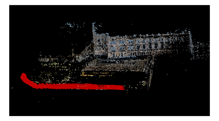
(a) Alcatraz Courtyard

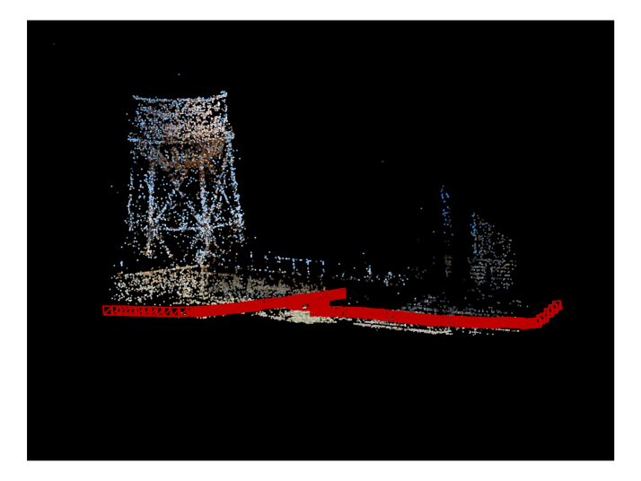
(b) Alcatraz Water Tower

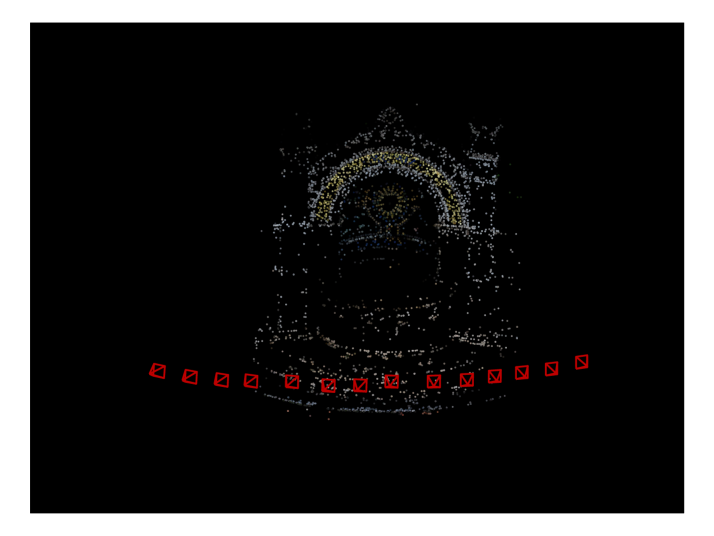
(c) Drinking Fountain Somewhere In Zurich

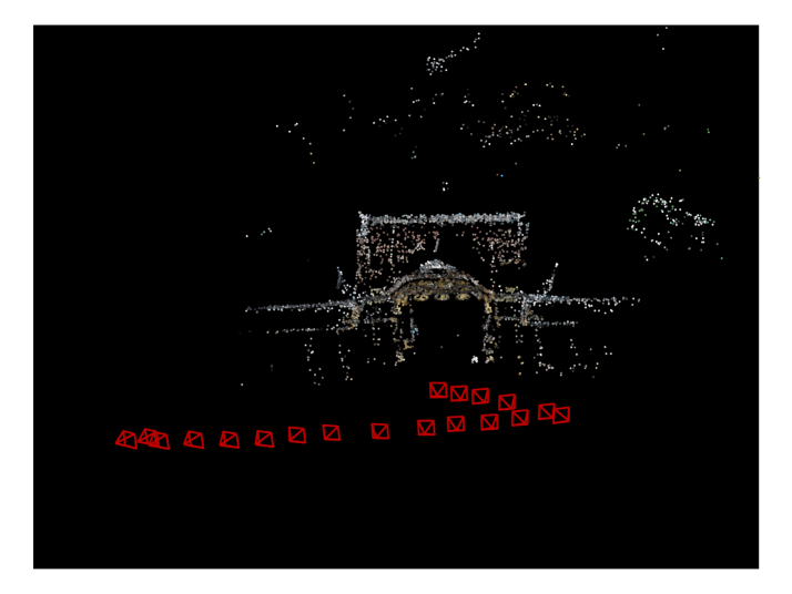
(d) Nijo Castle Gate

Figure 5: Single scene 3D reconstructions and recovery of camera parameters with our method. Each pair shows on the left the triangulated point cloud and the recovered camera locations and orientations (in red) and on the right one of the input images.

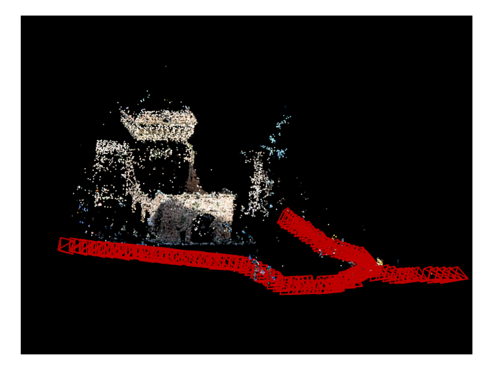
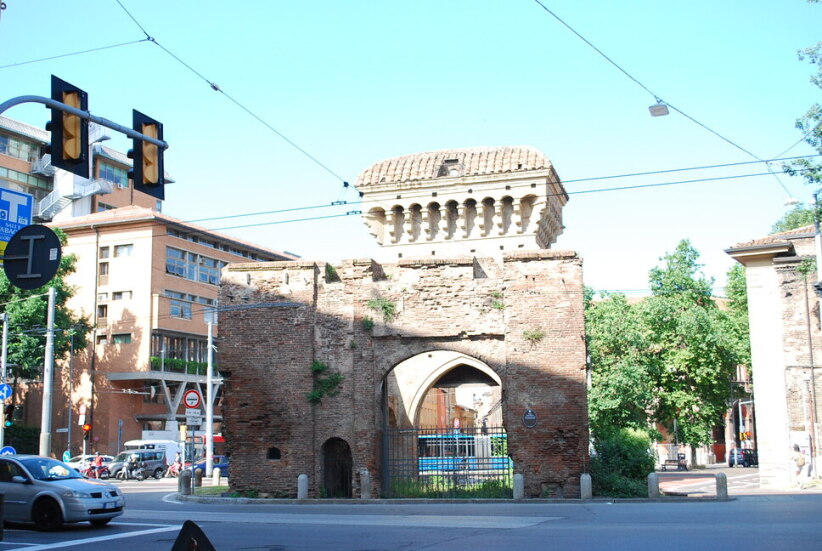
(a) Porta San Donato Bologna

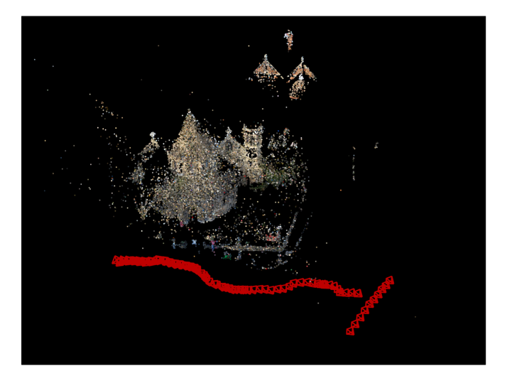
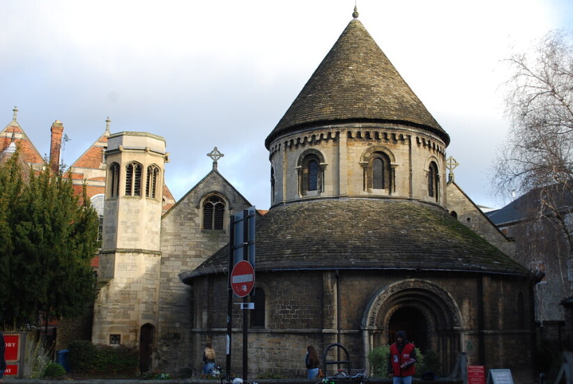
(b) Round Church Cambridge

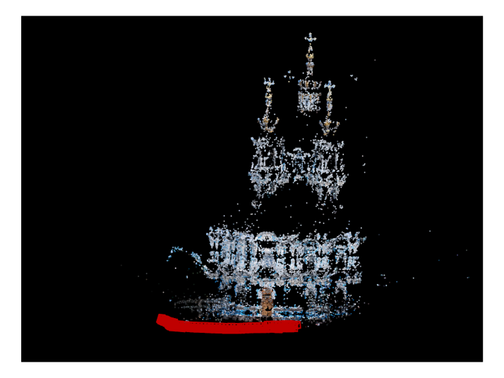
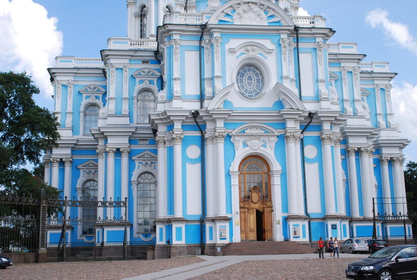
(c) Smolny Cathedral St Petersburg

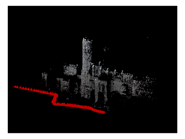
(d) Some Cathedral In Barcelona

Figure 7: Single scene 3D reconstructions and recovery of camera parameters with our method. Each pair shows on the left the triangulated point cloud and the recovered camera locations and orientations (in red) and on the right one of the input images.

(a) Sri Veeramakaliamman Singapore

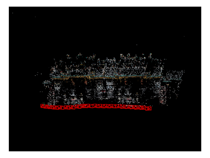
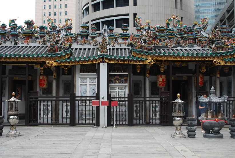
(b) Yueh Hai Ching Temple Singapore

Figure 9: Single scene 3D reconstructions and recovery of camera parameters with our method. Each pair shows on the left the triangulated point cloud and the recovered camera locations and orientations (in red) and on the right one of the input images.

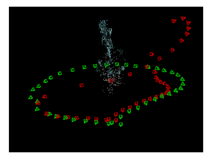
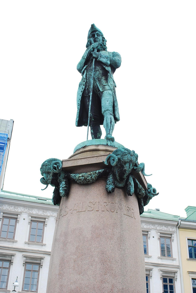
Figure 11: A failure case. Single scene 3D reconstruction and recovery of camera parameters with our method applied to Jonas Ahlstromer (reprojection error 8.41 pixels). The left image shows the triangulated point cloud, the recovered camera locations and orientations (in red) and the ground truth camera locations and orientations (in green). The right image is one of the input images.

Epoch 0

Epoch 2000

Epoch 5000

Epoch 10000

Epoch 15000

Epoch 20000

Epoch 25000

Epoch 35000

Epoch 45000

Epoch 60000

Epoch 70000

After BA

Figure 12: 3D structure and camera parameter evolution during the optimization of the network.

Learning from multiple scenes.

Figures 14 and 16 show reconstruction results using our model before and after bundle adjustment in 3 scenarios: (i) inference using our trained model (ii) inference followed by fine tuning and (iii) short run of optimization. Table 9 shows execution times for our trained model. We note that using inference only yields a good initialization for bundle adjustment in a small fraction of a second. Using fine tuning yields more accurate results (See Table 2 in the paper) with execution times similar to Colmap. The short optimization generally yields less accurate results with execution times similar to fine tuning, emphasizing the importance of the trained model.

Scan #Images #Points Time (seconds) Inference Fine tuning BA Colmap Alcatraz Courtyard 133 23674 $0.007$ $199.125$ $43.512$ $286.0$ Alcatraz Water Tower 172 14828 $0.007$ $110.847$ $26.44$ $130.0$ Drinking Fountain Somewhere In Zurich 14 5302 $0.007$ $20.302$ $2.925$ $16.0$ Nijo Castle Gate 19 7348 $0.008$ $24.493$ $4.308$ $21.0$ Porta San Donato Bologna 141 25490 $0.007$ $194.651$ $45.416$ $170.0$ Round Church Cambridge 92 84643 $0.014$ $360.97$ $90.092$ $229.0$ Smolny Cathedral St Petersburg 131 51115 $0.004$ $534.528$ $101.456$ $516.0$ Some Cathedral In Barcelona 177 30367 $0.007$ $208.542$ $55.424$ $451.0$ Sri Veeramakaliamman Singapore 157 130013 $0.319$ $291.727$ $242.888$ $583.0$ Yueh Hai Ching Temple Singapore 43 13774 $0.004$ $45.458$ $10.539$ $106.0$ Scan #Images #Points Time (seconds) Inference Fine tuning BA GPSFM Alcatraz Water Tower 172 14828 $0.055$ $89.646$ $68.939$ $137.057$ Dino 319 36 319 $0.004$ $8.151$ $0.475$ $3.253$ Dino 4983 36 4983 $0.122$ $7.66$ $2.21$ $4.994$ Dome 85 84792 $0.203$ $160.896$ $76.867$ $105.837$ Drinking Fountain 14 5302 $0.01$ $18.197$ $3.016$ $3.348$ Gustav Vasa 18 4249 $0.007$ $14.435$ $2.766$ $3.449$ Nijo 19 7348 $0.013$ $34.397$ $3.121$ $6.37$ Skansen Kronan 131 28371 $0.141$ $197.531$ $63.853$ $93.831$ Some Cathedral In Barcelona 177 30367 $0.133$ $185.984$ $47.597$ $110.485$ Sri Veeramakaliamman Singapore 157 130013 $0.314$ $473.294$ $195.374$ $301.713$

Table 9: Execution times for our trained model. The table shows execution times in seconds in the calibrated (left) and uncalibrated (right) settings.

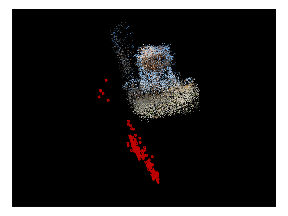
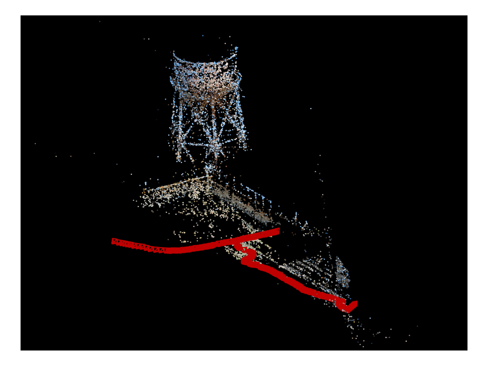
(a) Inference before (left) and after (right) BA

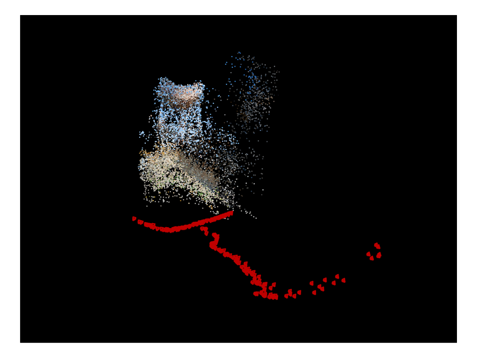
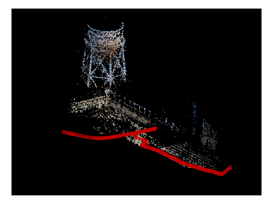
(b) Inference + fine tuning before (left) and after (right) BA

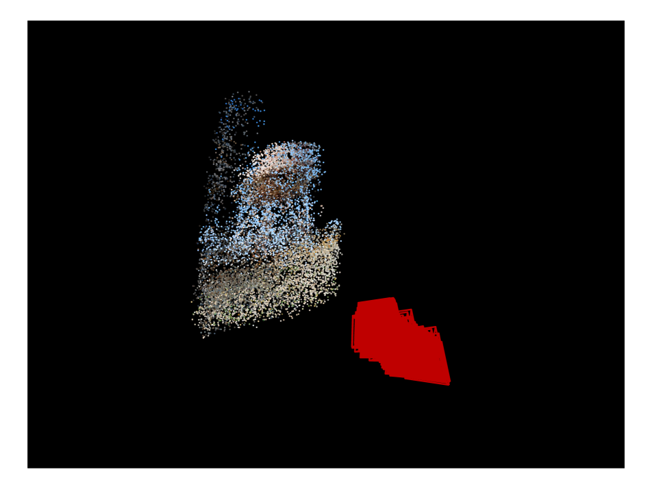
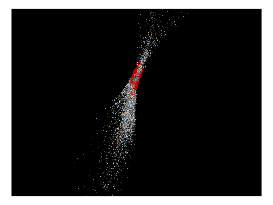
(c) Short optimization before (left) and after (right) BA

Figure 14: Alcatraz Water Tower. Reconstruction with our trained model. The figure shows results of inference (top row) and inference followed by fine tuning (middle row) before BA (left) and after BA (right). The bottom row shows the result of the short optimization strategy (starting with a random initialization). Each panel shows the recovered cameras positions (in red) and the recovered 3D points, corresponding to the point tracks. It can be seen that in this case accurate reconstruction can be obtained either by pure inference or inference followed by fine tuning (+ BA). In contrast, short optimization failed to accurately recover camera positions, leading to failure of the BA.

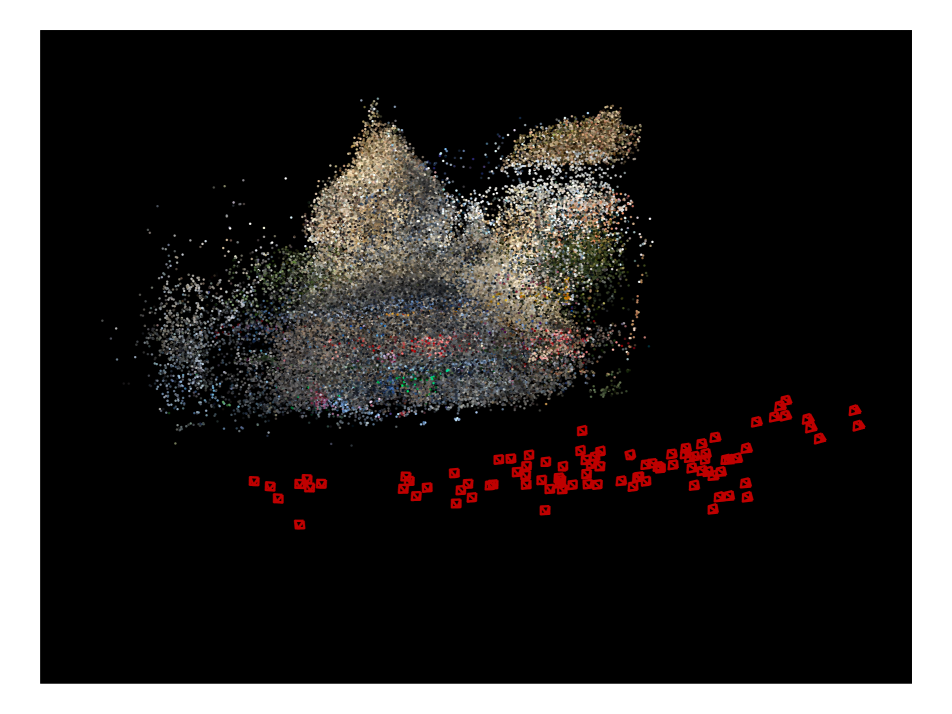
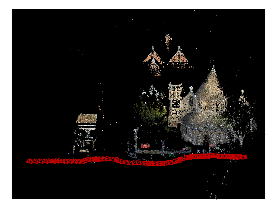
(a) Inference before (left) and after (right) BA

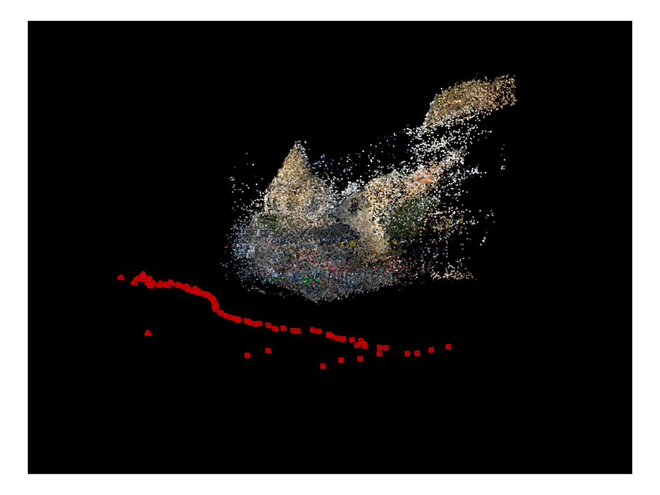
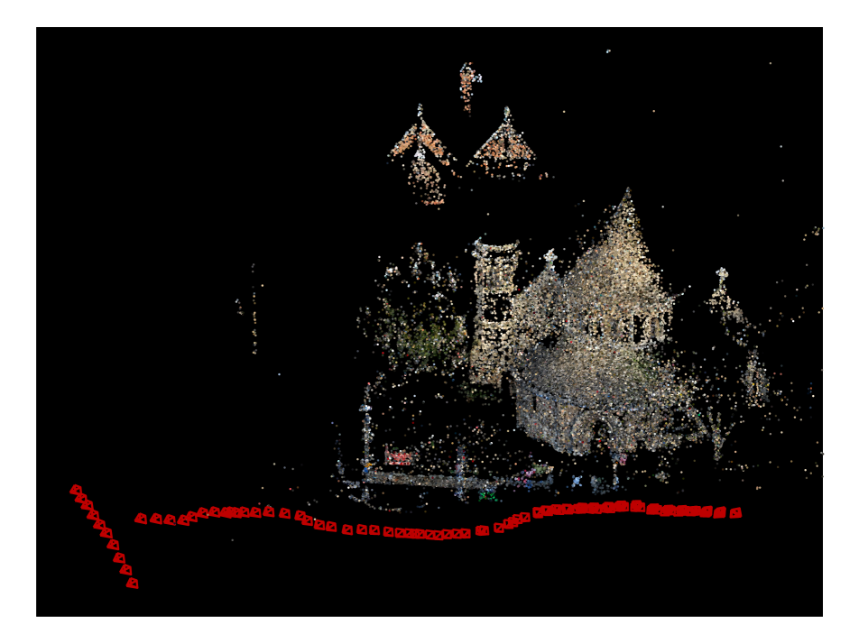
(b) Inference + fine tuning before (left) and after (right) BA

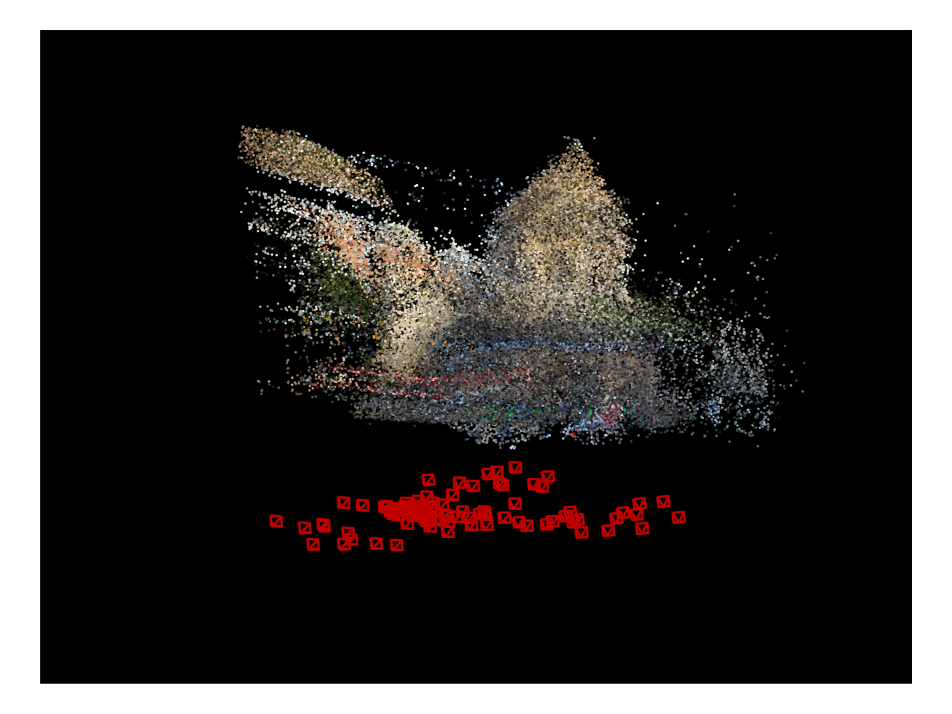
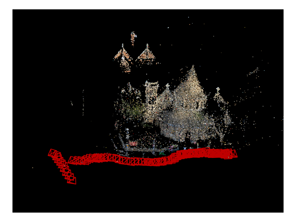
(c) Short optimization before (left) and after (right) BA

Figure 16: Round Church Cambridge. Reconstruction with our trained model. The figure shows results of inference (top row) and fine tuning (middle row) before BA (left) and after BA (right). The bottom row shows the result of the short optimization (starting with a random initialization). Each panel shows the recovered cameras positions (in red) and 3D points. Here fine tuning + BA yielded the most accurate reconstruction.

References

- [1] Sameer Agarwal, Keir Mierle, and Others. Ceres solver. http://ceres-solver.org.
- [2] Mica Arie-Nachimson, Shahar Z Kovalsky, Ira Kemelmacher-Shlizerman, Amit Singer, and Ronen Basri. Global motion estimation from point matches. In 2012 Second International Conference on 3D Imaging, Modeling, Processing, Visualization & Transmission, pages 81–88. IEEE, 2012.
- [3] Federica Arrigoni, Beatrice Rossi, Pasqualina Fragneto, and Andrea Fusiello. Robust synchronization in so(3) and se(3) via low-rank and sparse matrix decomposition. Computer Vision and Image Understanding, 174:95–113, 2018.
- [4] Rianne van den Berg, Thomas N Kipf, and Max Welling. Graph convolutional matrix completion. arXiv preprint arXiv:1706.02263, 2017.
- [5] Tolga Birdal, Michael Arbel, Umut Simsekli, and Leonidas J Guibas. Synchronizing probability measures on rotations via optimal transport. In Proceedings of the IEEE/CVF Conference on Computer Vision and Pattern Recognition, pages 1569–1579, 2020.
- [6] Avishek Chatterjee and Venu Madhav Govindu. Efficient and robust large-scale rotation averaging. In Proceedings of the IEEE International Conference on Computer Vision, pages 521–528, 2013.
- [7] Xuelian Cheng, Yiran Zhong, Mehrtash Harandi, Yuchao Dai, Xiaojun Chang, Tom Drummond, Hongdong Li, and Zongyuan Ge. Hierarchical neural architecture search for deep stereo matching, 2020.
- [8] Stéphane Christy and Radu Horaud. Euclidean shape and motion from multiple perspective views by affine iterations. IEEE Trans. on Pattern Analysis and Machine Intelligence, 18(11):1098–1104, 1996.
- [9] Taco Cohen and Max Welling. Group equivariant convolutional networks. In International conference on machine learning, pages 2990–2999. PMLR, 2016.
- [10] Yuchao Dai, Hongdong Li, and Mingyi He. Projective multiview structure and motion from element-wise factorization. IEEE Trans. on Pattern Analysis and Machine Intelligence, 35(9):2238–2251, 2013.
- [11] Anders Eriksson, Carl Olsson, Fredrik Kahl, and Tat-Jun Chin. Rotation averaging and strong duality. In Proceedings of the IEEE Conference on Computer Vision and Pattern Recognition, pages 127–135, 2018.
- [12] Carlos Esteves, Christine Allen-Blanchette, Ameesh Makadia, and Kostas Daniilidis. Learning so (3) equivariant representations with spherical cnns. In Proceedings of the European Conference on Computer Vision (ECCV), pages 52–68, 2018.
- [13] Matthias Fey and Jan Eric Lenssen. Fast graph representation learning with pytorch geometric. arXiv preprint arXiv:1903.02428, 2019.
- [14] Amnon Geifman, Yoni Kasten, Meirav Galun, and Ronen Basri. Averaging essential and fundamental matrices in collinear camera settings. In Proceedings of the IEEE/CVF Conference on Computer Vision and Pattern Recognition, pages 6021–6030, 2020.
- [15] Justin Gilmer, Samuel S Schoenholz, Patrick F Riley, Oriol Vinyals, and George E Dahl. Neural message passing for quantum chemistry. In International Conference on Machine Learning, pages 1263–1272. PMLR, 2017.
- [16] Jason S. Hartford, Devon R. Graham, Kevin Leyton-Brown, and Siamak Ravanbakhsh. Deep models of interactions across sets. In ICML, 2018.
- [17] Richard I Hartley. In defense of the eight-point algorithm. IEEE Transactions on pattern analysis and machine intelligence, 19(6):580–593, 1997.
- [18] Richard. I. Hartley and Andrew Zisserman. Multiple View Geometry in Computer Vision. Cambridge University Press, second edition, 2004.
- [19] Je Hyeong Hong and Christopher Zach. pose: Pseudo object space error for initialization-free bundle adjustment. In Proceedings of the IEEE Conference on Computer Vision and Pattern Recognition, pages 1876–1885, 2018.
- [20] Je Hyeong Hong, Christopher Zach, and Andrew Fitzgibbon. Revisiting the variable projection method for separable nonlinear least squares problems. In 2017 IEEE Conference on Computer Vision and Pattern Recognition (CVPR), pages 5939–5947. IEEE, 2017.
- [21] Je Hyeong Hong, Christopher Zach, Andrew Fitzgibbon, and Roberto Cipolla. Projective bundle adjustment from arbitrary initialization using the variable projection method. In European Conference on Computer Vision, pages 477–493. Springer, 2016.
- [22] Po-Han Huang, Kevin Matzen, Johannes Kopf, Narendra Ahuja, and Jia-Bin Huang. Deepmvs: Learning multi-view stereopsis. In IEEE Conference on Computer Vision and Pattern Recognition (CVPR), 2018.
- [23] Nianjuan Jiang, Zhaopeng Cui, and Ping Tan. A global linear method for camera pose registration. In Proceedings of the IEEE International Conference on Computer Vision, pages 481–488, 2013.
- [24] Abhishek Kar, Christian Häne, and Jitendra Malik. Learning a multi-view stereo machine. In I. Guyon, U. V. Luxburg, S. Bengio, H. Wallach, R. Fergus, S. Vishwanathan, and R. Garnett, editors, Advances in Neural Information Processing Systems, volume 30, pages 365–376, 2017.
- [25] Yoni Kasten, Amnon Geifman, Meirav Galun, and Ronen Basri. Algebraic characterization of essential matrices and their averaging in multiview settings. In Proceedings of the IEEE International Conference on Computer Vision, pages 5895–5903, 2019.
- [26] Yoni Kasten, Amnon Geifman, Meirav Galun, and Ronen Basri. Gpsfm: Global projective sfm using algebraic constraints on multi-view fundamental matrices. In Proceedings of the IEEE Conference on Computer Vision and Pattern Recognition, pages 3264–3272, 2019.
- [27] Alex Kendall, Matthew Grimes, and Roberto Cipolla. Posenet: A convolutional network for real-time 6-dof camera relocalization. In Proceedings of the IEEE international conference on computer vision, pages 2938–2946, 2015.
- [28] Ryan Kennedy, Laura Balzano, Stephen J Wright, and Camillo J Taylor. Online algorithms for factorization-based structure from motion. Computer Vision and Image Understanding, 150:139–152, 2016.
- [29] Risi Kondor and Shubhendu Trivedi. On the generalization of equivariance and convolution in neural networks to the action of compact groups. In International Conference on Machine Learning, pages 2747–2755. PMLR, 2018.
- [30] Juho Lee, Yoonho Lee, Jungtaek Kim, Adam Kosiorek, Seungjin Choi, and Yee Whye Teh. Set transformer: A framework for attention-based permutation-invariant neural networks. In International Conference on Machine Learning, pages 3744–3753. PMLR, 2019.
- [31] Yang Lin, Li Yang, Zhouchen Lin, Tong Lin, and Hongbin Zha. Factorization for projective and metric reconstruction via truncated nuclear norm. In 2017 International Joint Conference on Neural Networks (IJCNN), pages 470–477. IEEE, 2017.
- [32] H. Christopher. Longuet-Higgins. A computer algorithm for reconstructing a scene from two projections. Nature, 293, 1981.
- [33] Ludovic Magerand and Alessio Del Bue. Practical projective structure from motion (p2sfm). In Proceedings of the IEEE International Conference on Computer Vision, pages 39–47, 2017.
- [34] Haggai Maron, Heli Ben-Hamu, Nadav Shamir, and Yaron Lipman. Invariant and equivariant graph networks. arXiv preprint arXiv:1812.09902, 2018.
- [35] Haggai Maron, Ethan Fetaya, Nimrod Segol, and Yaron Lipman. On the universality of invariant networks. In International conference on machine learning, pages 4363–4371. PMLR, 2019.
- [36] Haggai Maron, Or Litany, Gal Chechik, and Ethan Fetaya. On learning sets of symmetric elements. In International Conference on Machine Learning, pages 6734–6744. PMLR, 2020.
- [37] Daniel Martinec and Tomas Pajdla. Robust rotation and translation estimation in multiview reconstruction. In 2007 IEEE Conference on Computer Vision and Pattern Recognition, pages 1–8. IEEE, 2007.
- [38] John Oliensis and Richard Hartley. Iterative extensions of the sturm/triggs algorithm: Convergence and nonconvergence. IEEE Trans. on Pattern Analysis and Machine Intelligence, 29(12):2217–2233, 2007.
- [39] Carl Olsson and Olof Enqvist. Stable structure from motion for unordered image collections. In Scandinavian Conf. on Image Analysis, pages 524–535. Springer, 2011.
- [40] Onur Ozyesil and Amit Singer. Robust camera location estimation by convex programming. In Proceedings of the IEEE Conference on Computer Vision and Pattern Recognition (CVPR), June 2015.
- [41] Onur Özyeşil, Vladislav Voroninski, Ronen Basri, and Amit Singer. A survey of structure from motion. Acta Numerica, 26:305–364, 2017.
- [42] Adam Paszke, Sam Gross, Francisco Massa, Adam Lerer, James Bradbury, Gregory Chanan, Trevor Killeen, Zeming Lin, Natalia Gimelshein, Luca Antiga, et al. Pytorch: An imperative style, high-performance deep learning library. In Advances in neural information processing systems, pages 8026–8037, 2019.
- [43] Pulak Purkait, Tat-Jun Chin, and Ian Reid. Neurora: Neural robust rotation averaging. arXiv preprint arXiv:1912.04485, 2019.
- [44] Charles R Qi, Hao Su, Kaichun Mo, and Leonidas J Guibas. Pointnet: Deep learning on point sets for 3d classification and segmentation. In Proceedings of the IEEE conference on computer vision and pattern recognition, pages 652–660, 2017.
- [45] Siamak Ravanbakhsh, Jeff Schneider, and Barnabas Poczos. Deep learning with sets and point clouds. arXiv preprint arXiv:1611.04500, 2016.
- [46] Siamak Ravanbakhsh, Jeff Schneider, and Barnabas Poczos. Equivariance through parameter-sharing. In International Conference on Machine Learning, pages 2892–2901. PMLR, 2017.
- [47] Johannes Lutz Schönberger and Jan-Michael Frahm. Structure-from-motion revisited. In Conference on Computer Vision and Pattern Recognition (CVPR), 2016.
- [48] Johannes L Schönberger, Enliang Zheng, Jan-Michael Frahm, and Marc Pollefeys. Pixelwise view selection for unstructured multi-view stereo. In European Conference on Computer Vision, pages 501–518. Springer, 2016.
- [49] Johannes L. Schönberger. Colmap code. https://colmap.github.io/.
- [50] Soumyadip Sengupta, Tal Amir, Meirav Galun, Tom Goldstein, David W Jacobs, Amit Singer, and Ronen Basri. A new rank constraint on multi-view fundamental matrices, and its application to camera location recovery. In Proceedings of the IEEE Conference on Computer Vision and Pattern Recognition, pages 4798–4806, 2017.
- [51] Noah Snavely, Steven M Seitz, and Richard Szeliski. Photo tourism: exploring photo collections in 3d. In ACM Siggraph 2006 Papers, pages 835–846. 2006.
- [52] Peter Sturm and Bill Triggs. A factorization based algorithm for multi-image projective structure and motion. In European Conf. on computer vision, pages 709–720. Springer, 1996.
- [53] Chengzhou Tang and Ping Tan. Ba-net: Dense bundle adjustment network. arXiv preprint arXiv:1806.04807, 2018.
- [54] Roberto Tron, Xiaowei Zhou, and Kostas Daniilidis. A survey on rotation optimization in structure from motion. In Proceedings of the IEEE Conference on Computer Vision and Pattern Recognition (CVPR) Workshops, June 2016.
- [55] Toshio Ueshiba and Fumiaki Tomita. A factorization method for projective and euclidean reconstruction from multiple perspective views via iterative depth estimation. In European Conf. on computer vision, pages 296–310. Springer, 1998.
- [56] Benjamin Ummenhofer, Huizhong Zhou, Jonas Uhrig, Nikolaus Mayer, Eddy Ilg, Alexey Dosovitskiy, and Thomas Brox. Demon: Depth and motion network for learning monocular stereo. In Proceedings of the IEEE Conference on Computer Vision and Pattern Recognition, pages 5038–5047, 2017.
- [57] Oxford VGG. Multiview datasets. http://www.robots.ox.ac.uk/~vgg/data/.
- [58] Sudheendra Vijayanarasimhan, Susanna Ricco, Cordelia Schmid, Rahul Sukthankar, and Katerina Fragkiadaki. Sfm-net: Learning of structure and motion from video, 2017.
- [59] Renhao Wang, Marjan Albooyeh, and Siamak Ravanbakhsh. Equivariant maps for hierarchical structures. arXiv preprint arXiv:2006.03627, 2020.
- [60] Zirui Wang, Shangzhe Wu, Weidi Xie, Min Chen, and Victor Adrian Prisacariu. NeRF: Neural radiance fields without known camera parameters. arXiv preprint arXiv:2102.07064, 2021.
- [61] Xingkui Wei, Yinda Zhang, Zhuwen Li, Yanwei Fu, and Xiangyang Xue. Deepsfm: Structure from motion via deep bundle adjustment, 2020.
- [62] Kyle Wilson and Noah Snavely. Robust global translations with 1dsfm. In European Conference on Computer Vision, pages 61–75. Springer, 2014.
- [63] Daniel E Worrall, Stephan J Garbin, Daniyar Turmukhambetov, and Gabriel J Brostow. Harmonic networks: Deep translation and rotation equivariance. In Proceedings of the IEEE Conference on Computer Vision and Pattern Recognition, pages 5028–5037, 2017.
- [64] Changchang Wu. Towards linear-time incremental structure from motion. In 2013 International Conference on 3D Vision-3DV 2013, pages 127–134. IEEE, 2013.
- [65] Keyulu Xu, Weihua Hu, Jure Leskovec, and Stefanie Jegelka. How powerful are graph neural networks? arXiv preprint arXiv:1810.00826, 2018.
- [66] Yao Yao, Zixin Luo, Shiwei Li, Tian Fang, and Long Quan. Mvsnet: Depth inference for unstructured multi-view stereo. In Proceedings of the European Conference on Computer Vision (ECCV), September 2018.
- [67] Lior Yariv, Yoni Kasten, Dror Moran, Meirav Galun, Matan Atzmon, Basri Ronen, and Yaron Lipman. Multiview neural surface reconstruction by disentangling geometry and appearance. Advances in Neural Information Processing Systems, 33, 2020.
- [68] Manzil Zaheer, Satwik Kottur, Siamak Ravanbakhsh, Barnabas Poczos, Ruslan R Salakhutdinov, and Alexander J Smola. Deep sets. In Advances in neural information processing systems, pages 3391–3401, 2017.
- [69] Tinghui Zhou, Matthew Brown, Noah Snavely, and David G. Lowe. Unsupervised learning of depth and ego-motion from video. In Proceedings of the IEEE Conference on Computer Vision and Pattern Recognition (CVPR), pages 6612–6619, 2017.