The inverse spectral problem for quantum semitoric systems

Abstract

Given a quantum semitoric system composed of pseudodifferential operators, Berezin-Toeplitz operators, or a combination of both, we obtain explicit formulas for recovering, from the semiclassical asymptotics of the joint spectrum, all symplectic invariants of the underlying classical semitoric system.

Our formulas are based on the possibility to obtain good quantum numbers for joint eigenvalues from the bare data of the joint spectrum. In the spectral region corresponding to regular values of the momentum map, the algorithms developed by Dauge, Hall and the second author [27] produce such labellings. In our proof, it was crucial to extend these algorithms to the boundary of the spectrum, which led to the new notion of asymptotic half-lattices, and to globalize the resulting labellings.

Using the construction given by Pelayo and the second author in [79], our results prove that semitoric systems are completely spectrally determined in an algorithmic way : from the joint spectrum of a quantum semitoric system one can construct a representative of the isomorphism class of the underlying classical semitoric system. In particular, this recovers the uniqueness result obtained by Pelayo and the authors in [62, 61], and completes it with the explicit computation of all invariants, including the twisting index.

In the cases of the spin-oscillator and the coupled angular momenta, we implement the algorithms and illustrate numerically the computation of the invariants from the joint spectrum.

1 Introduction

The goal of this paper is to answer the question “can one hear a semitoric system?”, which belongs to a long lineage of inverse spectral problems popularized by Kac in his famous article [53]. As often, the aim is to recover a classical geometry, up to isomorphism, from the data of a discrete set obtained as a quantum spectrum.

Semitoric systems form a class of completely integrable Hamiltonian systems with two degrees of freedom. Their introduction as a mathematical object, more than 15 years ago, was motivated both by symplectic geometry [89] and quantum physics [93]. Indeed, they play a fundamental role in explaining stable couplings between two particles, through the celebrated Jaynes-Cummings model and its variants [51]. For instance, an atom, seen as a multi-spin system, trapped in a potential cavity, is a semitoric system of great importance in entanglement experiments and quantum computing (constructing and controlling quantum dots), as explained in the colloquium paper by Raimond-Brune-Haroche [82]. Semitoric systems can describe numerous models, from a photon in an optical cavity to a symmetric molecule near a relative equilibrium, and have been widely used in quantum chemistry and spectrocopy, see [84, 52] and references therein. The precise structure of the quantum spectrum of semitoric systems, in particular its “non-linear” behaviour with respect to the harmonic oscillator ladder, has been used as a proof of the true quantum mechanical nature of matter-light interaction [41], and it was suggested that this spectral feature should also impact the dynamical control of quantum dots. Recently, the spectral structure of a seemingly different model (Rydberg-dressed atoms) was used to propose an “experimental isomorphism” with the classical Jaynes-Cummings sytem [63].

On the mathematical side, semitoric systems have been extensively studied in the last 15 years (see for instance the review [3]), and the intriguing connections between the spectra of quantum semitoric systems and the symplectic geometry of the underlying classical systems have been a driving force in the development of the theory. Thus, naturally, when a complete set of “numerical” symplectic invariants of classical semitoric systems was discovered [78, 79], the question was raised of whether these invariants were spectrally determined. This was stated in [80, Conjecture 9.1], further advertised in several papers as the inverse spectral conjecture for semitoric systems (see for instance [85], [10, Section 7.2] or the recent surveys [3, 70], and the references therein), and investigated in particular in [77, 62, 61, 19, 71]. The aim of the current article is to give explicit formulas and algorithms to obtain all the invariants from the spectrum. This provides a complete proof of the aforementioned conjecture.

Before giving detailed definitions in the next sections, let us simply mention, in this introduction, that a semitoric system on a 4-dimensional symplectic manifold $(M,\omega)$ is a pair of commuting Hamiltonians $F=(J,H)$ on $M$, where $J$ is the momentum map of an effective $S^{1}$-action, and $F:M\to\mathbb{R}^{2}$, viewed as a singular Lagrangian fibration, has singularities of a certain Morse-Bott type, with compact, connected fibers. These systems are of course very natural from the physical viewpoint where $S^{1}$-symmetry is ubiquitous and can be seen mathematically as a surprisingly far-reaching generalization of the toric systems studied by Atiyah, Guillemin-Sternberg, Delzant [5, 43, 28] and many others. Then, the symplectic invariants of $F$, which completely characterize $(M,\omega,F)$ [78, 79], are a sequence of numbers and combinatorial objects that describe the associated singular integral affine structure; and these invariants can be expressed as five objects, with some mutual relations:

1. A rational, convex polygonal set $\Delta\subset\mathbb{R}^{2}$.

2. A discrete set of distinguished points $c_{j}\in\Delta$, representing the isolated critical points (the focus-focus singularities) of $F$.

3. Each point $c_{j}$ is decorated with the following:

   1. a real number representing a symplectic volume (usually called the height invariant);

   2. an integer $k\in\mathbb{Z}$ called the twisting number;

   3. a formal Taylor series in two indeterminates.

A quantum semitoric system is a pair of commuting selfadjoint operators (quantum Hamiltonians), depending on the semiclassical parameter $\hbar$, whose joint principal symbol is $F$ as above, acting on a Hilbert space quantizing the symplectic manifold $(M,\omega)$. It defines a joint spectrum, which is a set of points in $\mathbb{R}^{2}$, and the natural inverse spectral problem is to recover the classical system $(M,\omega,F)$, up to symplectic equivalence, from the raw data of this point set as $\hbar\to 0$. This question naturally originates from quantum spectroscopy, where it is crucial to recover the nature of molecules through the observation of their spectrum; it is still a very active area of research, with many approaches and algorithms for detection; see for instance [83]. In this paper we shall adopt a semiclassical viewpoint, which takes advantage of symplectic invariants in phase space and was already advocated in [46].

One of the first results concerning the inverse spectral conjecture was to solve the particular case of toric systems [19, 71], where only the first invariant (the polygon) subsists. This was crucially based on Delzant’s theorem [28] (since the polygon is obtained explicitly as the semiclassical limit of the joint spectrum), and on the properties of Berezin-Toeplitz quantization, or more general quantizations for [71]. Naturally, the techniques were not transferable to more general cases, for which the main challenge is the treatment of focus-focus singularities, which do not appear in toric systems. Remark that, even when $M$ is fixed and when there is only one focus-focus singularity, the moduli space of semitoric systems on $M$ immediately becomes infinite dimensional. In [77], it was proven that the last invariant, the Taylor series, was spectrally determined, in the sense of a uniqueness statement: if two systems have the same quantum spectrum, then their Taylor series must coincide. Finally, the best result (prior to the present work) was obtained by Pelayo and the authors in [62, 61] and is also a uniqueness statement: based on the former cited article, it was proven in [62, Theorem A] that two quantum semitoric systems having the same joint spectrum (modulo $\mathscr{O}(\hbar^{2})$) must share the same invariants, with possibly the exception of the twisting index. As a consequence [61, Theorem B’], two Jaynes-Cummings systems (semitoric systems with only one critical fiber) with the same quantum spectrum and the same twisting number must be symplectically isomorphic. However, it was not known whether the twisting number could be determined from the spectrum, or not.

In this paper, we focus on the constructive part of the semitoric inverse spectral conjecture. Our main result can be informally stated as follows.

Theorem 1.1 (Theorem 3.6)

From the joint spectrum (modulo $\mathscr{O}(\hbar^{2})$) in a vertical strip of bounded width $S\subset\mathbb{R}^{2}$ of a quantum semitoric system, one can compute, in an algorithmic way, all symplectic invariants of the underlying classical semitoric system in $F^{-1}(S)$.

Using the construction given by Pelayo and the second author in [79], this completes the proof the inverse spectral conjecture for general semitoric systems (with an arbitrary number of focus-focus singularities).

Corollary 1.2

If two quantum semitoric systems have the same spectrum, then their underlying classical systems are symplectically isomorphic.

This corollary completes the result previously obtained by Pelayo and the authors in [62, 61]. The word “quantum” in these statements refers to both $\hbar$-pseudodifferential and Berezin-Toeplitz quantizations, which respectively appear in the quantization of cotangent bundles and compact symplectic manifolds. To the authors’ knowledge, this is the first algorithmic inverse spectral result that holds for a large class of quantum integrable systems on a possibly compact phase space, with possibly non-toric dynamics. Recall that in the specific case of compact toric systems, the result was proven by recovering the associated Delzant polytope [19, 71].

The uniqueness result of [62, 61] implies that, within the class of Jaynes-Cummings systems, the symplectic invariants other than the twisting index are implicitly determined by the asymptotics of the joint spectrum. In view of this, and the above discussion, the main achievements of the present work are to consider the whole class of semitoric systems, and within this class:

1. to constructively recover the twisting number associated with each focus-focus critical value (Theorem 5.1);

2. to constructively recover the full Taylor series invariant associated with each focus-focus critical value (Theorem 6.12);

3. to find a global procedure to construct the polygon invariant from the spectral data (Theorem 5.13);

4. to obtain an explicit formula that gives the height invariant from the joint spectrum (Proposition 6.1).

It is known from the classification of semitoric systems that the first and third item are not independent, since changing the polygon invariant implies a global shift of all the twisting numbers; hence the procedures to obtain them from the joint spectrum are intricate. In proving the second item, we additionally recover for the first time the full infinite jet of the Eliasson diffeomorphism, which brings the system near a focus-focus singularity into a Morse-Bott normal form and is known to be an invariant of the map $F$, see for instance [85, Definition 4.37]. In fact, the Taylor series and the Eliasson diffeomorphism are not specific to semitoric systems: they are invariants of a singular Lagrangian fibration near a focus-focus fiber, and our techniques allow to compute them explicitly from the joint spectrum of any quantum integrable system possessing such a singularity.

For the sake of completeness, we have also included the proof of some Bohr-Sommerfeld rules that were missing in the literature, in particular for Berezin-Toeplitz operators in the case of a transversally elliptic singularity. However, it is worth noticing that our strategy does not necessitate the more delicate uniform description of the joint spectrum in a neighborhood of a focus-focus singularity, which has been proved for $\hbar$-pseudodifferential operators [91] but is still conjectural for Berezin-Toeplitz operators (see also [6]). This can be circumvented by taking two consecutive limits, one as $\hbar\to 0$ for a given regular value $c$, then one as $c$ goes to the focus-focus value.

Recently, a renewal of interest on semitoric invariants was triggered by their explicit (algebraic and numerical) computations in a large number of important examples [76, 60, 2, 1]. Thus, we also wanted to take advantage of this to test our results on several cases, by implementing numerical algorithms along the proof of the theoretical results. This also means that in most of the proofs, we put some emphasis on practical formulas, errors and convergence rates.

Our proof is a combination of microlocal analysis, asymptotic analysis, symplectic geometry, but also, and crucially, combinatorial and algorithmic techniques borrowed from the recent work [27]. That work, motivated by detecting the rotation number on the joint spectrum of a quantum integrable system, introduced general tools for dealing with so-called asymptotic lattices of eigenvalues; these tools turned out to be essential in our approach. Indeed, contrary to the usual cases of inverse spectral theory where the spectral data is a sequence of real (and hence ordered) eigenvalues, here we have to deal with joint spectra of commuting operators, which are two-dimensional point clouds, moving with the semiclassical parameter. Thus, the first step in all our results is to consistently define good quantum numbers for such joint eigenvalues. Coming up with these quantum numbers is already non trivial near a regular value of the underlying momentum map where these eigenvalues are a deformation of the standard lattice, see [27]. Here, it will be crucial not only to develop a local-to-global theory of quantum numbers (because the presence of focus-focus singularities is known to obstruct the existence of global labellings), but also to obtain good labels near transversally elliptic singular values as well; in this case the joint spectrum is a deformation of the intersection of the standard lattice with a half-plane, which leads us to introduce the notion of asymptotic half-lattice.

In the aforementioned article, the emphasis was put on $\hbar$-pseudodifferential operators. In our case however, it is very important to also consider Berezin-Toeplitz operators, since many relevant examples of semitoric systems are defined on compact symplectic manifolds. Throughout this manuscript, we will make sure that the results that we use hold in both contexts.

Some general ideas of proof were already present in [81]. We were able to make some of them concrete. However, in that paper, the difficulty for finding good labellings for the joint spectrum was overlooked, and no strategy was given for the twisting index, since at that time the relationship between that invariant and the Taylor series was not understood.

The structure of the article is as follows.

• In Section 2, we recall the essential properties of semitoric systems and present their symplectic invariants in a new way which is more adapted to the inverse problem.

• In Section 3, we introduce a notion of semiclassical operators which allows us to deal with $\hbar$-pseudodifferential operators and Berezin-Toeplitz operators simultaneously. Then we define quantum semitoric systems and their joint spectra, and state our main result; Sections 4 to 7 are devoted to its proof.

• In Section 4, we review asymptotic lattices and their labellings, define and study asymptotic half-lattices, and show how to construct global labellings for unions of asymptotic lattices and half-lattices.

• In Section 5, we explain how to compute the twisting number and the semitoric polygon from the joint spectrum, effectively recovering the twisting index invariant.

• In Section 6, we give a procedure to obtain explicitly the height invariant, the full Taylor series invariant and the full infinite jet of the Eliasson diffeomorphism from the spectral data.

• In Section 7, we give a proof of the Bohr-Sommerfeld rules near an elliptic-transverse critical value of an integrable system, valid both for $\hbar$-pseudodifferential operators and Berezin-Toeplitz operators.

• In Section 8, we illustrate numerically the various formulas giving the symplectic invariants on two distinct examples (one on a compact manifold and one on a non-compact manifold).

• In the Appendix, we briefly review $\hbar$-pseudodifferential and Berezin-Toeplitz operators, emphasizing the non-compact cases required for our analysis.

Remark 1.3 The presentation of the classifying space of semitoric systems by means of the five invariants mentioned above has proven quite useful in the development of the inverse theory, allowing various studies to focus on a particular item; but the separation between the five invariants is somewhat arbitrary. For instance, the last three invariants 3a, 3b, and 3c, could be naturally combined into a single Taylor series (see Section 2.5). This was already partly observed in [4]; in [69] the authors even prefer to pack all invariants into a single object. However, it makes sense to single out the last one (the Taylor series invariant), as it is the complete semi-global invariant for a neighborhood of the critical fiber associated with $c_{j}$, not only for semitoric systems, but also for any integrable system with a simple focus-focus singularity [95] (this was used in [77] to show that the joint spectrum near the singular value determines the semi-global classification). On the contrary, the height invariant and the twisting number characterize the global location of the fiber within the whole system.

Actually, while the main goal of our work is to solve the inverse problem for semitoric systems, it is interesting to notice that a large part of our analysis, which concerns the Taylor series invariant and the Eliasson diffeomorphism, is local in action variables and hence not specific to semitoric systems.   $\triangle$

Remark 1.4 As mentioned above, the present article goes beyond the uniqueness statement of the inverse problem by proposing a constructive approach. Therefore, the methods in play are necessarily quite different from those used in the previous inverse spectral results [77] and [62]. As a consequence, in addition to completely solving the inverse spectral conjecture, our analysis also provides a new proof of the main results of these articles.   $\triangle$

Remark 1.5 After their original definition and classification, several natural generalizations of semitoric systems have been proposed [73, 48, 69, 97]. It would be interesting to investigate the inverse problem for the generalized classes, and in particular in the case of multiple pinches in the focus-focus fibers [74, 69], because in this case a negative answer seems plausible.   $\triangle$

Remark 1.6 There are many interesting connections between semiclassical inverse spectral theory of quantum integrable systems, as presented here, and other inverse spectral problems in geometric analysis and PDEs; on this matter, we refer the reader to the existing literature; see for instance [94] and references therein for a quick and recent survey. Let us simply recall two salient aspects.

The first one concerns the inverse spectral theory of the Riemannian Laplacian, certainly the most well-known of all inverse spectral problems; see the survey [26]. In that case, semiclassical asymptotics are clearly present through the high-energy limit, and the consequences of $S^{1}$-invariant geometry (surfaces of revolution) have been derived in important cases, see [99, 32]. In order to completely fill the gap between these types of systems and the semitoric framework, one would need to lift the properness assumption on the $S^{1}$-momentum map $J$, which is one of the generalizations alluded to in the previous remark 1.2.

The second one concerns the generalization of inverse problems from Schrödinger operators to general Hamiltonians, see [50]; in that paper, a “Taylor series” plays an important role, and comes from a Birkhoff normal form. This is related (although in an indirect fashion, see [38]) to our Taylor series and the Eliasson diffeomorphism discussed in Section 2.5. The use of such formal series in inverse problems was already crucial in Zelditch’s milestone paper [100]. Under a toric hypothesis, this formal series can disappear [31], giving way to more geometric invariants like Delzant polytopes. In our semitoric case, we need to combine both worlds: Birkhoff-type invariants and toric-type invariants.   $\triangle$

2 Symplectic invariants of semitoric systems

In this section, we give a new formula to compute the twisting number in relation with the Eliasson diffeomorphism and the linear part of the Taylor series invariant (see Lemma 2.7 and Proposition 2.14), which will be crucial for our analysis of the joint spectrum. We also describe all the other symplectic invariants of semitoric integrable systems introduced in [78, 79] (see also [85] for a more recent account).

2.1 Symplectic preliminaries

We endow $\mathbb{R}^{4}$ with canonical coordinates $(x_{1},x_{2},\xi_{1},\xi_{2})$ and the standard symplectic form $\omega_{0}=d\xi_{1}\wedge dx_{1}+d\xi_{2}\wedge dx_{2}$. If $(M,\omega)$ is a four-dimensional symplectic manifold and $m\in M$, there always exist local Darboux coordinates $(x_{1},x_{2},\xi_{1},\xi_{2})$ centered at $m$ in which $\omega=\omega_{0}$. If $f\in C^{\infty}(M;\mathbb{R})$, we define the Hamiltonian vector field $\mathcal{X}_{f}$ as the unique vector field such that $\operatorname{d}\!{f}+\omega(\mathcal{X}_{f},\cdot)=0$. The Poisson bracket of two functions $f,g\in C^{\infty}(M;\mathbb{R})$ is defined as $\{f,g\}=\omega(\mathcal{X}_{f},\mathcal{X}_{g})$.

A Liouville integrable system on the four-dimensional symplectic manifold $(M,\omega)$ is the data of two functions $J,H\in C^{\infty}(M;\mathbb{R})$ such that $\{J,H\}=0$ and $\mathcal{X}_{J},\mathcal{X}_{H}$ are almost everywhere linearly independent. In this article, we will use the terminology “integrable system” for “Liouville integrable system”. The map $F=(J,H):M\to\mathbb{R}^{2}$ is called the momentum map of the system. A point $m\in M$ where the above linear independence condition holds (which is equivalent to the linear independence of $\operatorname{d}\!{J}$ and $\operatorname{d}\!{H}$) is called a regular point of $F$; otherwise, $m$ is called a critical point of $F$. A point $c\in\mathbb{R}^{2}$ is called a regular value of $F$ if $F^{-1}(c)$ contains only regular points, and a critical value of $F$ otherwise.

Let $(M,\omega,F=(J,H))$ be an integrable system on a four-dimensional manifold, and let $c\in\mathbb{R}^{2}$ be a regular value of the momentum map $F$. The action-angle theorem [66] (see also [35]) states that if $F^{-1}(c)$ is compact and connected, then there exist a local diffeomorphism $G_{0}:(\mathbb{R}^{2},0)\to(\mathbb{R}^{2},c)$ and a local symplectomorphism $\phi$ from a neighborhood of $m\in M$ to a neighborhood of $0\in T^{*}\mathbb{T}^{2}$ with coordinates $(\theta_{1},\theta_{2},I_{1},I_{2})$ and symplectic form $\operatorname{d}\!{I_{1}}\wedge\operatorname{d}\!{\theta_{1}}+\operatorname{d}\!{I_{2}}\wedge\operatorname{d}\!{\theta_{2}}$ such that $F\circ\phi^{-1}=G_{0}(I_{1},I_{2})$. Our convention is $\mathbb{T}^{2}=\mathbb{R}^{2}/(2\pi\mathbb{Z})^{2}$, so that the angles $\theta_{i}$ belong to $\mathbb{R}/2\pi\mathbb{Z}$.

It is standard to call $I_{1},I_{2}$ action variables; in what follows, we call $G_{0}^{-1}$ an action diffeomorphism. These are not unique; if $A\in\mathrm{GL}(2,\mathbb{Z})$ and $\kappa\in\mathbb{R}^{2}$, and if we let

$$\begin{pmatrix}L_{1}\\ L_{2}\end{pmatrix}=A\begin{pmatrix}I_{1}\\ I_{2}\end{pmatrix}+\kappa,$$ (1)

then $(L_{1},L_{2})$ is another set of action variables near $m$, and every pair of action variables is obtained in this fashion. We will mainly be interested in the case where $G_{0}^{-1}$ is an oriented action diffeomorphism, i.e. satisfying ${\rm d}G_{0}(0)>0$; in this case the above statements remain true with $A\in\mathrm{SL}(2,\mathbb{Z})$.

Action diffeomorphisms define a natural integral affine structure on the set of regular values of $F$; recall that an integral affine manifold of dimension $d$ is a smooth manifold with an atlas whose transition maps are of the form $A\cdot+b$ where $A\in\mathrm{GL}(d,\mathbb{Z})$ and $b\in\mathbb{R}^{d}$.

2.2 Semitoric systems

There exists a notion of non-degenerate critical point of an integrable system which we will not describe here, see [11, Section 1.8]. A consequence of this definition is the following symplectic analogue of the Morse lemma, which we state here only in dimension four:

Theorem 2.1 (Eliasson normal form [39])

Let $(M,\omega,F=(J,H))$ be an integrable system on a four-dimensional manifold and let $m\in M$ be a non-degenerate critical point of $F$. Then there exist local symplectic coordinates $(x,\xi)=(x_{1},x_{2},\xi_{1},\xi_{2})$ on an open neighborhood $U\subset M$ of $m$ and $Q=(q_{1},q_{2}):U\to\mathbb{R}^{2}$ whose components $q_{i}$ belong to the following list:

• $q_{i}(x,\xi)=\frac{1}{2}(x_{i}^{2}+\xi_{i}^{2})$ (elliptic),

• $q_{i}(x,\xi)=x_{i}\xi_{i}$ (hyperbolic),

• $q_{i}(x,\xi)=\xi_{i}$ (regular),

• $q_{1}(x,\xi)=x_{1}\xi_{2}-x_{2}\xi_{1}$, $q_{2}(x,\xi)=x_{1}\xi_{1}+x_{2}\xi_{2}$ (focus-focus),

such that $m$ corresponds to $(x,\xi)=(0,0)$ and $\{J,q_{i}\}=0=\{H,q_{i}\}$ for every $i\in\{1,2\}$. Furthermore, if none of these components is hyperbolic, there exists a local diffeomorphism $g:(\mathbb{R}^{2},0)\to(\mathbb{R}^{2},F(m))$ such that for every $(x,\xi)\in U$, $F(x,\xi)=(g\circ Q)(x,\xi)$.

Strictly speaking, a complete proof of this theorem was published only for analytic Hamiltonians [90], and for $C^{\infty}$ Hamiltonians in several cases: the fully elliptic case in any dimension [33, 40], the focus-focus case in dimension $4$ [96, 14], the general (hyperbolic and elliptic) case in dimension 2 [23]. Based on this theorem, the extension to partial action-angle coordinates corresponding to the regular components $\xi_{i}$, or in the presence of additional compact group action, was proven in [68].

A semitoric system $(M,\omega,F=(J,H)))$ is the data of a connected four-dimensional symplectic manifold $(M,\omega)$ and smooth functions $J,H:M\to\mathbb{R}$ such that

1. $(J,H)$ is a Liouville integrable system,

2. $J$ generates an effective Hamiltonian $S^{1}$-action,

3. $J$ is proper,

4. $F$ has only non-degenerate singularities with no hyperbolic components.

Remark 2.2 The properness of $J$ implies that of the momentum map $F$; while the properness of $F$ is crucial throughout the analysis, that of $J$ itself can be seen as a technical condition, enabling the use of Morse theory. It implies in particular that the fibres of $F$ and $J$ are connected, see [93]. However, in order to include classical examples from mechanics, like the spherical pendulum, which live on cotangent bundles, it would be important to relax this assumption. First steps in this direction were made in [72, 73]; in [27], the properness of $J$ was not assumed. In this work, however, we shall keep this assumption, because in most places we rely on the classification of semitoric systems, which only exists for proper $J$.   $\triangle$

Consequently, a semitoric system only displays singularities of elliptic-elliptic, elliptic-regular (commonly called elliptic-transverse) and focus-focus type. A semitoric system is called simple if each level set of $J$ contains at most one focus-focus point. Throughout the rest of the article, we will always assume that semitoric systems are simple.

Definition 2.3 ([78])

Two semitoric systems $(M,\omega,F)$ and $(M^{\prime},\omega^{\prime},F^{\prime})$ are isomorphic if there exist a symplectomorphism $\varphi:(M,\omega)\to(M^{\prime},\omega^{\prime})$ and a smooth map $g(x,y)=(x,f(x,y))$, with $\partial_{y}f>0$, such that

$$F^{\prime}\circ\varphi=g\circ F.$$

The main result of [78] is to exhibit a list of concrete invariants such that two semitoric systems that possess the same set of invariants are isomorphic. Then [79] shows how to construct a semitoric system given an arbitrary choice of invariants. Let us now introduce these invariants more precisely.

Let $(M,\omega,F=(J,H))$ be a simple semitoric system. Its first symplectic invariant is the number $m_{f}\in\mathbb{N}$ of focus-focus singularities. If $m_{f}=0$, i.e. if the system is of toric type, the only remaining invariant is the semitoric polygon.

2.3 Semitoric polygons

We first assume that $m_{f}\geq 1$ and denote by $(x_{1},y_{1}),\ldots,(x_{m_{f}},y_{m_{f}})$ the images of the focus-focus singularities by $F$, numbered in such a way that $x_{1}<\ldots<x_{m_{f}}$. Let $B_{\mathrm{reg}}$ be the set of regular values of $F$. The polygonal invariant is given as an equivalence class of convex polygonal sets; each representative in this class can be constructed after making a choice of initial action diffeomorphism and cut directions $\vec{\epsilon}\in\{-1,1\}^{m_{f}}$. (In the non-compact case, these polygons are not bounded in general, and the terms convex polygon will have the meaning given in [85, Definition 5.19]; in particular a convex polygon has a discrete set of vertices.)

More precisely, let $\vec{\epsilon}=(\epsilon_{1},\ldots,\epsilon_{m_{f}})\in\{-1,1\}^{m_{f}}$ and, for $i\in\{1,\ldots,m_{f}\}$, let $\ell_{i}^{\epsilon_{i}}=\{(x_{i},y)\ |\ \epsilon_{i}y\geq\epsilon_{i}y_{i}\}$ be the vertical half-line starting at $(x_{i},y_{i})$ and going upwards if $\epsilon_{i}=1$ and downwards if $\epsilon_{i}=-1$. Finally, let $\ell^{\vec{\epsilon}}=\cup_{i=1}^{m_{f}}\ell_{i}^{\epsilon_{i}}$. By [93, Theorem 3.8], there exists a homeomorphism $\Phi_{\vec{\epsilon}}:F(M)\to\Phi_{\vec{\epsilon}}(F(M))\subset\mathbb{R}^{2}$ whose restriction to $F(M)\setminus\ell^{\vec{\epsilon}}$ is a diffeomorphism into its image, of the form

$$\Phi_{\vec{\epsilon}}(x,y)=\left(x,\Phi_{\vec{\epsilon}}^{(2)}(x,y)\right),\qquad\frac{\partial\Phi_{\vec{\epsilon}}^{(2)}}{\partial y}>0,$$ (2)

whose image $\Delta_{\vec{\epsilon}}=\Phi_{\vec{\epsilon}}(F(M))$ is a convex polygon, which sends the integral affine structure of $B_{\mathrm{reg}}\setminus\ell^{\vec{\epsilon}}$ given by action-angle coordinates to the standard integral affine structure on $\mathbb{R}^{2}$, and extends to a smooth multivalued map from $B_{\mathrm{reg}}$ to $\mathbb{R}^{2}$ such that for any $i\in\{1,\ldots,m_{f}\}$ and for any $c\in\ell_{i}^{\epsilon_{i}}\setminus\{(x_{i},y_{i})\}$,

$$\lim_{\begin{subarray}{c}(x,y)\to c\\ x<x_{i}\end{subarray}}\operatorname{d}\!{\Phi}_{\vec{\epsilon}}=T\lim_{\begin{subarray}{c}(x,y)\to c\\ x>x_{i}\end{subarray}}\operatorname{d}\!{\Phi}_{\vec{\epsilon}},\qquad T=\begin{pmatrix}1&0\\ 1&1\end{pmatrix}.$$

Following [85], such a homeomorphism $\Phi_{\vec{\epsilon}}$ is called a cartographic homeomorphism. For a given $\vec{\epsilon}$, it is unique modulo left composition by an element of the subgroup $\mathcal{T}$ of $GL(2,\mathbb{Z})\ltimes\mathbb{R}^{2}$ consisting of the composition of $T^{k}$ for some $k\in\mathbb{Z}$ and a vertical translation. Indeed, a cartographic homeomorphism is constructed from action variables above $B_{\mathrm{reg}}$, and this degree of freedom corresponds to the choice of initial action variables of the form $(J,L)$.

One can formalize the action of changing cut directions as follows. For $x_{0}\in\mathbb{R}$ and $n\in\mathbb{N}$, let $t_{x_{0}}^{n}:\mathbb{R}^{2}\to\mathbb{R}^{2}$ be the map defined as the identity on $\{x\leq x_{0}\}$ and as $T^{n}$ (relative to any choice of origin on the line $\{x=x_{0}\}$) on $\{x\geq x_{0}\}$. For $\vec{x}=(x_{1},\ldots,x_{s})\in\mathbb{R}^{s}$ and $\vec{n}=(n_{1},\ldots,n_{s})\in\mathbb{N}^{s}$, let $t_{\vec{n},\vec{x}}=t_{x_{1}}^{n_{1}}\circ\ldots\circ t_{x_{s}}^{n_{s}}$. Let $\vec{\epsilon},\vec{\epsilon^{\prime}}\in\{-1,1\}^{m_{f}}$ and let $\Delta_{\vec{\epsilon}}$, $\Delta_{\vec{\epsilon^{\prime}}\star\vec{\epsilon}}$ be the two polygons constructed as above with the same initial set of action variables and the two choices of cut directions $\vec{\epsilon}$ and $\vec{\epsilon^{\prime}}\star\vec{\epsilon}=\left(\epsilon_{1}^{\prime}\epsilon_{1},\ldots,\epsilon_{m_{f}}^{\prime}\epsilon_{m_{f}}\right)$. Then one may check that

$$\Delta_{\vec{\epsilon^{\prime}}\star\vec{\epsilon}}=t_{\vec{u},\vec{x}}(\Delta_{\vec{\epsilon}}),\qquad\vec{u}=\left(\frac{\epsilon_{1}-\epsilon_{1}\epsilon_{1}^{\prime}}{2},\ldots,\frac{\epsilon_{m_{f}}-\epsilon_{m_{f}}\epsilon_{m_{f}}^{\prime}}{2}\right),\quad\vec{x}=(x_{1},\ldots,x_{m_{f}}).$$

The polygonal invariant is the orbit of any of the convex polygons $\Delta_{\vec{\epsilon}}$ constructed as above under the action of $\mathcal{T}\times\{-1,1\}^{m_{f}}$. We will denote by $(\Delta_{\vec{\epsilon}},\Phi_{\vec{\epsilon}})$ the representative of this invariant constructed using $\Phi_{\vec{\epsilon}}$.

Finally, if $m_{f}=0$, this construction is still valid but there is no $\vec{\epsilon}$, no cut direction and the invariant is the orbit of any of the polygons under the action of $\mathcal{T}$, see [85, Section 5.2.2] for more details.

2.4 Twisting number and twisting index

In this section, we express the definition of the twisting numbers and twisting index for a simple semitoric integrable system $(M,\omega,F=(J,H))$ on a four-dimensional manifold, in terms of a geometric object that we call the radial curve (Definition 2.6). The construction we use here is somewhat different from the initial definition in [78], and more adapted to the inverse problem.

We first introduce the twisting number, an integer associated with each focus-focus singularity $m_{0}\in M$ of $F$. In order to simplify notation, we may let $F(m_{0})=0$. By assumption, $m_{0}$ is the only singularity of the connected critical fiber $\Lambda_{0}:=F^{-1}(0)$. Let $\Omega_{0}\subset M$ be a saturated neighborhood of $\Lambda_{0}$; then one can show that $F(\Omega_{0})\subset\mathbb{R}^{2}$ is a neighborhood of the origin. Let $B\subset F(\Omega_{0})$ be a small ball centered at the origin, such that $B\setminus\{0\}$ consists of regular values of $F_{|\Omega_{0}}$.

Let $U\subset B\setminus\{0\}$ be a simply connected open set. Let us choose oriented action coordinates in $F^{-1}(U)$ of the form $I=(J,L)$. Recall from (1) (and the fact that the first component, $J$, must be preserved) that $L$ is not unique, but any other choice can only be of the form $L^{\prime}=L+nJ+c$, for some $n\in\mathbb{Z}$ and $c\in\mathbb{R}$. Nevertheless, there are two natural ways of selecting $L$. One comes from the global geometry of the momentum map, and consists in choosing the affine coordinates used in the construction of the semitoric polygon (Section 2.3): $I$ must coincide with $\Phi_{\vec{\epsilon}}\circ F$, where $\Phi_{\vec{\epsilon}}$ is the cartographic map (2) (so this depends on the choice of a representative $\Delta_{\vec{\epsilon}}$ of the polygon invariant). We will use the notation $L_{\Phi_{\vec{\epsilon}}}$ for this global choice. Then, there is a local choice $L_{\textup{priv}}$, which is dictated by the singular behaviour on $\Lambda_{0}$, and which was called ‘privileged action variable’ in [78, Definition 5.7].

Definition 2.4

The integer $p\in\mathbb{Z}$ such that ${\rm d}L_{\Phi_{\vec{\epsilon}}}={\rm d}L_{\textup{priv}}+p\ {\rm d}J$ is called the twisting number corresponding to the global choice of $L_{\Phi_{\vec{\epsilon}}}$.

Let us recall the definition of the privileged action variable $L_{\textup{priv}}$. Let $\Omega$ be a sufficiently small neighborhood of $m_{0}$ in $M$. In $\Omega$, the fiber $\Lambda_{0}\cap\Omega$ is the union of two surfaces intersecting transversally at $m_{0}$. For a generic Hamiltonian of the form $f(J,H)$, these surfaces respectively constitute the local stable and unstable manifolds for the flow of the associated Hamiltonian vector field, and on each of them, the trajectories tending to the fixed point $m_{0}$ are of ‘focus’ type, i.e. they are spirals that wind infinitely many times around $m_{0}$. However, Theorem 2.1 implies that there is a precise choice $f_{r}$ of $f$, which is unique up to sign, addition of a constant, and addition of a flat function, such that, in some local Darboux coordinates $(x_{1},x_{2},\xi_{1},\xi_{2})$,

$$f_{r}(J,H)=x_{1}\xi_{1}+x_{2}\xi_{2}.$$

(For the uniqueness, see [95, Lemma 4.1]). Let us call such $H_{r}:=f_{r}(J,H)$ the “radial” Hamiltonian, because its trajectories inside $\Lambda_{0}\cap\Omega$ are line segments tending to the origin in the above Darboux coordinates, and hence have intrinsically a zero winding number around $m_{0}$. Imposing $f_{r}(0)=0$ and $(J,H_{r})$ to be oriented with respect to $(J,H)$, meaning that $\partial_{H}f_{r}>0$, the function $f_{r}$ becomes unique, modulo addition of a flat function at $0\in\mathbb{R}^{2}$. The map $q:=(J,H_{r}):M\to\mathbb{R}^{2}$ is called the quadratic, or Eliasson momentum map, because, modulo the aforementioned uniqueness, it must coincide with the quadratic map $Q$ expressed in Eliasson’s coordinates (Theorem 2.1). Note that $q=g^{-1}\circ F$ with $g^{-1}(x,y)=(x,f_{r}(x,y))$.

Assume now that $U$ is contained in the open set $F(\Omega)$. Any vector field $\mathcal{X}$ in $\Omega\cap F^{-1}(U)$ that is tangent to the leaves of $F$ (i.e. included in the kernel of $\operatorname{d}\!{F}$) decomposes in a unique way as

$$\mathcal{X}=\tilde{\tau}_{1}\mathcal{X}_{J}+\tilde{\tau}_{2}\mathcal{X}_{H_{r}},$$ (3)

where $\tilde{\tau}_{1},\tilde{\tau}_{2}$ are smooth functions on the local leaf space, i.e. $\tilde{\tau}_{j}=F^{*}\tau_{j}$, where $\tau_{j}$ is smooth on $U$. Let $L:M\to\mathbb{R}$ be such that $(J,L)$ is a set of action coordinates. Since action diffeomorphisms form a flat sheaf, they admit a unique extension in any simply connected open subset of the set of regular values of $F$. In particular we can extend $L$ inside $F(\Omega)\setminus\ell$, where $\ell$ is the upward vertical half-line from the origin. We may apply the decomposition (3) to the Hamiltonian vector field $\mathcal{X}_{L}$ to get smooth functions $\tau_{1},\tau_{2}$ on $F(\Omega)\setminus\ell$.

Proposition 2.5 ([95],[85, Lemma 4.46])

Let $\log$ be the determination of the complex logarithm obtained by choosing arguments in $(-\frac{3\pi}{2},\frac{\pi}{2}]$. The functions

$$\begin{cases}\sigma_{1}:c\mapsto\tau_{1}(c)+\frac{1}{2\pi}\Im(\log(c_{1}+if_{r}(c_{1},c_{2}))),\\[5.69054pt] \sigma_{2}:c\mapsto\tau_{2}(c)+\frac{1}{2\pi}\Re(\log(c_{1}+if_{r}(c_{1},c_{2})))\end{cases}$$

extend smoothly at $c=(0,0)$.

It follows that $\tau_{1}$ is multivalued and that $\tau_{2}$ exhibits a logarithmic singularity. In order to deal with this, it will be convenient to study $\sigma_{1}$ and $\sigma_{2}$ along a special curve that we describe below.

Definition 2.6

The image by $F$ of the zero-set of $H_{r}$ in $\Omega$ is a local curve $\gamma_{r}$ given by the equation $f_{r}(x,y)=0$, which we call the radial curve.

From the implicit function theorem $\gamma_{r}$ is, locally near the origin, a graph parameterized by $x$, say the graph of $\varphi:\mathbb{R}\to\mathbb{R}$. Let $\Gamma$ be the intersection of $F(\Omega)$ with an open vertical half-plane whose boundary contains the origin. Shrinking $\Omega$ if necessary, we may assume that $\Gamma$ contains a branch of $\gamma_{r}$ accumulating at the origin. In what follows, we will always choose the half-plane defining $\Gamma$ to be the right half-plane.

Lemma 2.7

The function $\nu_{1}:x\mapsto\tau_{1}(x,\varphi(x))$, defined for $x>0$ (so that $(x,\varphi(x))\in\Gamma$), extends smoothly at $x=0$, and $\lim_{x\to 0^{+}}\nu_{1}(x)=\sigma_{1}(0)$.

Proof .  We know from Proposition 2.5 that the function $\sigma_{1}$ extends smoothly at the origin. But for $x>0$

$$\sigma_{1}(x,\varphi(x))=\nu_{1}(x)+\frac{1}{2\pi}\Im(\log(x+if_{r}(x,\varphi(x))))=\nu_{1}(x)+\frac{1}{2\pi}\Im(\log\ x)=\nu_{1}(x)$$

and $\varphi(0)=0$, so $\nu_{1}$ extends smoothly at $x=0$, with value $\sigma_{1}(0)$ at this point. $\square$

Remark 2.8 Observe that the choice of $\Gamma$ is indeed important: for $x<0$,

$$\nu_{1}(x)=\sigma_{1}(x,\varphi(x))-\frac{1}{2}\underset{x\to 0}{\longrightarrow}\sigma_{1}(0)-\frac{1}{2},$$

so choosing the left half-plane for $\Gamma$ would have shifted the above limit by a factor $\frac{1}{2}$.   $\triangle$

Because $f_{r}$ is unique up to a flat function, $\sigma_{1}(0)$ does not depend on any choice made but $L$. As remarked earlier, any other $L^{\prime}$ is of the form $L^{\prime}=L-nJ+c$ for some integer $n$ and some constant $c\in\mathbb{R}$, leading to $\tau_{1}^{\prime}=\tau_{1}-n$ and hence $\sigma_{1}^{\prime}(0)=\sigma_{1}(0)-n$. By definition, we call $L^{\prime}$ a privileged action variable and we denote it by $L_{\textup{priv}}$, when

$$\sigma_{1}^{\prime}(0)\in\interval[openright]01$$

and in this case we write $\sigma_{1}^{\textup{p}}$ instead of $\sigma_{1}^{\prime}$, to emphasize the fact that we are working with this privileged choice. Notice that a privileged action variable is defined only up to an additive constant $c$; one may fix its value if needed, see Equation (8) and the discussion below.

Summing up, given any fixed choice $L$ of action variable, defining $(\tilde{\tau}_{1},\tilde{\tau}_{2})=(F^{*}\tau_{1},F^{*}\tau_{2})$ by

$$\mathcal{X}_{L}=\tilde{\tau}_{1}\mathcal{X}_{J}+\tilde{\tau}_{2}\mathcal{X}_{H_{r}},$$ (4)

and letting $\sigma_{1}(0)$ be the limit of $\tau_{1}$ at the origin along the radial curve $\gamma_{r}$, we have $L_{\textup{priv}}=L-nJ$ where $n$ is the integer part of $\sigma_{1}(0)$; remark how this formula confirms that $L_{\textup{priv}}$ does not depend on the choice of $L$ (while $n$ does).

Definition 2.9

If we let $\vec{\epsilon}=(1,\ldots,1)$ and choose $\Phi_{\vec{\epsilon}}$ so that the twisting number of the focus-focus point $m_{0}$ vanishes, then $\Phi_{\vec{\epsilon}}$ is called the privileged cartographic map at $m_{0}$, and the corresponding polygon $\Delta_{\textup{priv}}^{m_{0}}:=\Phi_{\vec{\epsilon}}(F(M))$ is called the privileged polygon at $m_{0}$ for this semitoric system.

Remark 2.10 As explained earlier, this privileged polygon is defined up to a vertical translation (because the privileged action at $m_{0}$ is defined up to addition of a constant). Although one should keep this in mind, for simplicity we will often talk about the privileged polygon.   $\triangle$

We may now recall the definition of the twisting index, which is a global invariant taking into account all twisting numbers and the choice of a semitoric polygon. Using the notation of Section 2.3, given a choice of cartographic map $\Phi_{\vec{\epsilon}}$, we have $m_{f}$ twisting numbers $p_{1},\dots,p_{m_{f}}$. Each of them, individually, may be set to zero using its associated privileged cartographic map, but in general one cannot set all these numbers to zero simultaneously. The twisting index is precisely the equivalence class of the tuple $(p_{1},\dots,p_{m_{f}})$ modulo the choice of a cartographic map; see [78, Definition 5.9].

Remark 2.11 The twisting number $p$, being defined as an integer part, is sensitive to perturbations, see Figure 11 for an illustration of this fact. When a reference Hamiltonian $L$ is given, a better symplectic invariant of the triple $(J,H,L)$ is the coefficient $\sigma_{1}(0)$ itself. Its fractional part $\sigma_{1}^{\textup{p}}(0)=\sigma_{1}(0)-p$, which is independent of $L$, is the “second Taylor series invariant” of the foliation induced by $F=(J,H)$, as defined in [95]: see Section 2.5 below.   $\triangle$

Remark 2.12 Given a triple $(J,H,L)$ as in Remark 2.9, it follows directly from (4) that $-\tau_{1}$ is the rotation number of the radial Hamiltonian $H_{r}$ computed in the action variables $(J,L)$. From the point of view of the toric action induced by $(J,L)$, it can be further interpreted as follows. Let $\mu:=(J,L):M\to\mathbb{R}^{2}$; it is a toric momentum map, defined on the saturated open set $\Omega^{\prime}:=F^{-1}(U)$, with the notation of the beginning of this section. It defines an isomorphism between the space of symplectic vector fields $X_{\beta}$ in $\Omega^{\prime}$ that are tangent to the $F$-foliation, and closed one-forms $\beta$ on the affine space $\mu(\Omega^{\prime})\subset\mathbb{R}^{2}$, via the formula

$$\iota_{X_{\beta}}\omega=-\mu^{*}\beta.$$

Taking $\beta=-\tau_{1}\operatorname{d}\!{j}+\operatorname{d}\!{\ell}$, where $(j,\ell)$ are the canonical affine coordinates in $\mathbb{R}^{2}$, we see from (4) that $\iota_{\tilde{\tau}_{2}\mathcal{X}_{H_{r}}}\omega=-\mu^{*}\beta$; hence $\beta$ gives the direction of the radial vector field $\mathcal{X}_{H_{r}}$. Therefore, the tangent to $\gamma_{r}$, expressed in the coordinates $(j,\ell)$, is $\ker\beta$, i.e. the line spanned by the vector $(1,\tau_{1})$.   $\triangle$

Now let us relate $\tau_{1}$ with the original momentum map $F=(J,H)$. Define the functions $(\tilde{a}_{1},\tilde{a}_{2})=(F^{*}a_{1},F^{*}a_{2})$ in $\Gamma$ by

$$\mathcal{X}_{L}=\tilde{a}_{1}\mathcal{X}_{J}+\tilde{a}_{2}\mathcal{X}_{H},$$ (5)

and let $s:=-\partial_{x}f_{r}/\partial_{y}f_{r}$; the latter is the “slope” of the tangent to the level sets of $f_{r}$. In particular $s(0)$ is the slope of the tangent to $\gamma_{r}$ at the origin. Equating (4) with (5), we get

$$\begin{cases}a_{1}=\tau_{1}+\tau_{2}\partial_{x}f_{r}\\ a_{2}=\tau_{2}\partial_{y}f_{r},\end{cases}$$ (6)

which gives, in $\Gamma$,

$$\tau_{1}=a_{1}+sa_{2}.$$ (7)

Recall that $a_{1},a_{2},\tau_{1},\tau_{2}$ are all ill-defined (and really singular) at the origin, while $s$ is smooth in a neighborhood of $0$.

Remark 2.13 In the papers [76, 60], the notation was slightly different and the matrix

$$B=\begin{pmatrix}1&0\\ b_{1}&b_{2}\end{pmatrix}$$

such that $q=\mathrm{Hess}(B\circ F)$ was considered. We claim that

$$s(0)=-\frac{b_{1}}{b_{2}}.$$

Indeed, on the one hand we have that $B\circ F=(q_{1},b_{1}q_{1}+b_{2}H)$, which yields

$$(q_{1},q_{2})=(q_{1},b_{1}q_{1}+b_{2}\mathrm{Hess}(H)).$$

On the other hand, $(q_{1},q_{2})=g\circ F=(J,f_{r}(J,H))$, hence $(q_{1},q_{2})=(q_{1},f_{r}(q_{1},H))$. So we obtain that

$$\operatorname{d}\!{q}_{2}=\partial_{x}f_{r}(q_{1},H)\operatorname{d}\!{q}_{1}+\partial_{y}f_{r}(q_{1},H)\operatorname{d}\!{H},$$

and since $\operatorname{d}\!{q}_{1}$ and $\operatorname{d}\!{q}_{2}$ vanish at the origin, we finally get

$$q_{2}=\partial_{x}f_{r}(q_{1},H)q_{1}+\partial_{y}f_{r}(q_{1},H)\mathrm{Hess}(H)$$

plus a term that vanishes at the origin, so we identify $b_{1}=\partial_{x}f_{r}(0)$ and $b_{2}=\partial_{y}f_{r}(0)$.   $\triangle$

2.5 The Taylor series invariant

The Taylor series invariant is not specific to semitoric systems. It is the classifying invariant of any singular Lagrangian fibration around a focus-focus fiber [95], and has been used for instance in [88] to study rational blowdowns. However, in this article we specialize its definition to the semitoric case. (This is mainly a matter of simplifying notation, since a neighborhood of a focus-focus fiber is always isomorphic, in a natural sense, to a semitoric system.)

We keep the same notation as Section 2.4. In particular we fix a focus-focus point $m_{0}$, $(J,L)$ are action variables in $F^{-1}(U)$, and $U$ is a small simply connected open set close to the critical value $F(m_{0})=0\in\mathbb{R}^{2}$. We can write $L=\tilde{L}\circ q$, where $q=(J,H_{r})$ and $\tilde{L}=\tilde{L}(X,Y)$ is smooth. From (4) we have

$$\tilde{\tau}_{1}=\frac{\partial\tilde{L}}{\partial X}\circ q,\quad\tilde{\tau}_{2}=\frac{\partial\tilde{L}}{\partial Y}\circ q.$$

Thus, it follows from Proposition 2.5 that the function

$$S(X,Y):=\tilde{L}(X,Y)+\Im(w\ln w-w),$$ (8)

where $w:=X+iY$, extends to a smooth function $S$ in a neighborhood of $0$, with $g^{*}\operatorname{d}\!{S}=\sigma_{1}\operatorname{d}\!{c}_{1}+\sigma_{2}\operatorname{d}\!{c}_{2}$. We denote the Taylor series of $S$ at the origin by

$$S^{\infty}=\sum_{\ell,m\geq 0}S_{\ell,m}X^{\ell}Y^{m}.$$

The main result of [95] is that the equivalence class of $S^{\infty}$ in the quotient $\frac{\mathbb{R}[\![X,Y]\!]}{\mathbb{R}\oplus\mathbb{Z}X}$ is a complete symplectic invariant for the singular foliation defined by $F$, in a neighborhood of $\Lambda_{0}=F^{-1}(0)$. The first terms $[S_{1,0}]\in\mathbb{R}/\mathbb{Z}$ and $S_{0,1}\in\mathbb{R}$ are called the linear invariants (of this Taylor series).

Proposition 2.14

The linear invariants of the Taylor series and the quantities $\sigma_{1},\sigma_{2}$ introduced in Section 2.4 are related by

$$[S_{1,0}]=\sigma_{1}(0)\mod\mathbb{Z},\qquad S_{0,1}=\sigma_{2}(0),$$

and more precisely

$$S_{1,0}=\sigma_{1}^{\textup{p}}(0)+p,$$

with $\sigma_{1}^{\textup{p}}(0)\in\interval[openright]01$, and $p\in\mathbb{Z}$ is the twisting number associated with $m_{0}$ for the choice of the action variable $L$.

The link between the twisting index and the Taylor series was presented independently in [69].

The height invariant.

The constant term $S_{0,0}$ is irrelevant as far as the semi-global classification near $\Lambda_{0}$ is concerned. However, once the global picture is taken into account, there is a way to get a meaningful value $S_{0,0}>0$. Since $L$ is defined up to a constant, we may decide that $L=0$ where $H$ reaches its minimal value on the compact set $J^{-1}(0)$. We see from (8) that, if $X=0$ is fixed, and $Y\to 0$, the function $\tilde{L}(X,Y)$ must tend to $S_{0,0}$. With this convention, $S_{0,0}$ is precisely the height invariant defined in [78, Definition 5.2].

Remark 2.15 If we relax the orientation-preserving hypothesis for the image in $\mathbb{R}^{2}$ of the joint momentum maps, and also the orientation of the $S^{1}$ action (i.e. allowing to replace $J$ by $-J$), then we have an interesting finite group acting on all invariants, and in particular on the Taylor series. This was studied in [85].   $\triangle$

Remark 2.16 The reader should be aware that there are slight differences in convention and notation in the literature (regarding for instance the sign of the standard symplectic form on $\mathbb{R}^{4}$, the respective parts played by $q_{1}$ and $q_{2}$, the complex structure on $\mathbb{R}^{4}$, the choice of $\tau_{1}\in\mathbb{R}/\mathbb{Z}$ or $\tau_{1}\in\mathbb{R}/2\pi\mathbb{Z}$, etc.), resulting in possible differences in the value of the Taylor series invariant: difference by a multiplicative factor $2\pi$, change in sign, shift of $S_{1,0}$ by $\pm\frac{1}{4}$ (or $\pm\frac{\pi}{2}$ when working modulo $2\pi\mathbb{Z}$), etc. See [74, Remark 6.2] or [4, Remark 4.11]. Here we have mostly adopted the notation and convention from [85]; the thesis [4] is also an extremely reliable source for the computation of the symplectic invariants with comparable convention (up to normalization by $2\pi$).   $\triangle$

3 Quantum semitoric systems

What are the quantum analogues of semitoric systems? Of course, the “old” Jaynes-Cummings model from quantum optics was already a quantum semitoric system, and so were the models studied in [84]. The mathematical formulation of “quantized” semitoric systems is hence very natural, and follows the physics intuition, see [81]: a quantum semitoric system is a pair of commuting operators which should be semiclassical quantizations of the components of the momentum map of a semitoric system. Here we need to make all these statements very precise. The type of quantization that we use will depend on the underlying phase space. Throughout this article, we will consider the following three situations:

1. $(M,\omega)=(T^{*}X,\operatorname{d}\!{\lambda})$ where $X=\mathbb{R}^{2}$ or $X$ is a compact Riemannian surface and $\lambda$ is the Liouville one-form,

2. $(M,\omega)$ is a quantizable (see Appendix A.2) compact Kähler manifold of dimension four,

3. $(M,\omega)=(\mathbb{C}\times N,\omega_{0}\oplus\omega_{N})$ where $\omega_{0}$ is the standard symplectic form on $\mathbb{C}$ and $(N,\omega_{N})$ is a quantizable compact Kähler surface.

These three situations occur in concrete examples coming from physical problems. The coupled spin-oscillator system (see Section 8.1), or Jaynes-Cummings model, is of great relevance in quantum optics and quantum information [51, 86, 82, 6, 7, 45] and has also been studied from the mathematical viewpoint [76, 2]. Its classical phase space is $\mathbb{R}^{2}\times\mathbb{S}^{2}$, which corresponds to case (M3). The coupled angular momenta system (see Section 8.2) is defined on $\mathbb{S}^{2}\times\mathbb{S}^{2}$, hence belongs to case (M2). It was used in [84] in order to propose a systematic way to describe energy rearrangement between spectral bands in molecules, see also [29].

On $T^{*}\mathbb{S}^{2}$, the spherical pendulum [25] is not a semitoric system in the strict acceptance that we took in Section 2.2 (because the Hamiltonian generating the circle action is not proper) but possesses one focus-focus singularity. The same situation occurs for the “champagne bottle” on $T^{*}\mathbb{R}^{2}$ [20]. In fact, it is quite possible that all strict semitoric systems on a cotangent bundle must be of toric type (i.e. they don’t possess any focus-focus singularity); we already know from [55] that such a cotangent bundle must be $T^{*}\mathbb{R}^{2}$. In the cotangent case, allowing for a non-proper map $J$ would be important for future works (see [73]), and since many of our constructions here are local, we believe that they should be adaptable to that more general setting.

Remark 3.1 We do not consider here the case of $T^{*}\mathbb{S}^{1}\times N$ where $N$ is a smooth compact surface. In this case every semitoric system must be of toric type. Indeed, it follows from [93, Corollary 5.5] and [42, Theorem 3.1] that the presence of a focus-focus singularity forces the manifold to be simply connected.

More generally, we do not include the case of a system on a non-compact symplectic manifold which is neither a cotangent bundle nor $\mathbb{R}^{2}\times N$ with $N$ compact; it is unclear how to quantize such a phase space, although some progress has recently been made in this direction [56]. But we are not aware of any concrete example of semitoric system with at least one focus-focus point in this setting.   $\triangle$

To each of the three geometric situations, we shall consider a quantum version and its semiclassical limit. We will use the generic terminology “semiclassical operator” to encompass all cases, and refer to Appendix A for details.

Definition 3.2

A semiclassical operator is either:

1. In case (M1), a (possibly unbounded) $\hbar$-pseudodifferential operator acting on $\mathcal{H}_{\hbar}:=L^{2}(X)$.

2. In case (M2), a Berezin-Toeplitz operator acting on $\mathcal{H}_{\hbar}:=H^{0}(M,\mathscr{L}^{k}\otimes\mathscr{K})$, the space of holomorphic sections of high tensor powers of a suitable line bundle, possibly twisted with another line bundle; there, the semiclassical parameter is $\hbar=\frac{1}{k}$.

3. In case (M3), a (possibly unbounded) Berezin-Toeplitz operator acting on

   $$\mathcal{H}_{\hbar} :=H^{0}(\mathbb{C}\times N,\mathscr{L}_{0}^{k}\boxtimes(\mathscr{L}^{k}\otimes\mathscr{K}))\cap L^{2}(\mathbb{C}\times N,\mathscr{L}_{0}^{k}\boxtimes(\mathscr{L}^{k}\otimes\mathscr{K}))$$

   $$\simeq\mathcal{B}_{k}(\mathbb{C})\otimes H^{0}(N,\mathscr{L}^{k}\otimes\mathscr{K}),$$

   still with $\hbar=\frac{1}{k}$. Here $\mathcal{B}_{k}(\mathbb{C})$ is the Bargmann space with weight $\exp(-k|z|^{2})$.

In fact, the three cases can be seen as instances of general (not necessarily compact) Berezin-Toeplitz quantization. It is well-known, for instance, that Weyl pseudodifferential quantization on $\mathbb{R}^{2d}$ is equivalent to Berezin-Toeplitz quantization on $\mathbb{C}^{d}$. Although a fully general theory has not been developed yet, it is also known since [13] that, in a microlocal sense, contact Berezin-Toeplitz quantization is always equivalent to homogeneous pseudodifferential quantization.

In all cases, a semiclassical operator is actually a family of operators $\hat{H}_{\hbar}$ indexed by the semiclassical parameter $\hbar$, acting on a Hilbert space $\mathcal{H}_{\hbar}$ that may depend on $\hbar$ as well. Most importantly for us, a selfadjoint semiclassical operator $\hat{H}_{\hbar}$ has a principal symbol $H\in C^{\infty}(M;\mathbb{R})$, which does not depend on $\hbar$; conversely, for any classical Hamiltonian $H\in C^{\infty}(M;\mathbb{R})$ (with suitable control at infinity in non-compact cases) there exists a semiclassical operator $\hat{H}_{\hbar}$ whose principal symbol is $H$. Any other semiclassical operator $\hat{H}^{\prime}_{\hbar}$ with principal symbol $H$ is $\mathscr{O}(\hbar)$-close to $\hat{H}_{\hbar}$ in a suitable topology. See Appendix A.

Given two semiclassical operators $\hat{J}_{\hbar}$ and ${\hat{H}_{\hbar}}$, their commutator $\frac{i}{\hbar}[\hat{J}_{\hbar},\hat{H}_{\hbar}]$ is again a semiclassical operator, whose principal symbol is the Poisson bracket $\{J,H\}$. We say that $\hat{J}_{\hbar}$ and ${\hat{H}_{\hbar}}$ commute if their commutator vanishes. In this case, one can show that the spectral measures of the selfadjoint operators $\hat{J}_{\hbar}$ and ${\hat{H}_{\hbar}}$ commute in the usual sense [15].

Definition 3.3

A quantum integrable system $(\hat{J}_{\hbar},\hat{H}_{\hbar})$ is the data of two commuting semiclassical operators acting on $\mathcal{H}_{\hbar}$ whose principal symbols $J,H$ form a Liouville integrable system. If moreover $(J,H)$ is a semitoric integrable system, we say that $(\hat{J}_{\hbar},\hat{H}_{\hbar})$ is a semitoric quantum integrable system, or a quantum semitoric system.

Definition 3.4

The joint spectrum of a quantum integrable system $(\hat{J}_{\hbar},\hat{H}_{\hbar})$ is the support of the joint spectral measure (see for instance [65, Section 6.5]) of $\hat{J}_{\hbar}$ and ${\hat{H}_{\hbar}}$.

We shall only consider situations where the joint spectrum is discrete: joint eigenvalues are isolated, with finite multiplicity. This is of course automatic in the compact Berezin-Toeplitz case, since the Hilbert spaces $\mathcal{H}_{\hbar}$ are finite dimensional. In the non compact case, this can be seen as the quantum analogue of the properness condition on the momentum map $F=(J,H):M\to\mathbb{R}^{2}$; indeed the joint spectrum is discrete if and only if, for any compact subset of $\mathbb{R}^{2}$, the corresponding joint spectral projection is compact (i.e. of finite rank). In the pseudodifferential case, a convenient assumption that guarantees discreteness of the spectrum is the ellipticity at infinity of the operator $\hat{J}_{\hbar}^{2}+\hat{H}_{\hbar}^{2}$, see [15]. If this holds, we say that the quantum integrable system is proper, and in what follows we will always work with proper quantum integrable systems.

We will need to compare families of spectra up to $\mathscr{O}(\hbar^{2})$. By this we mean the following (for an example of why this definition is relevant, see Remark 3.8 in [27]).

Definition 3.5

Let $A_{\hbar},B_{\hbar}\subset\mathbb{R}^{2}$ be two families of closed subsets indexed by $\hbar\in\mathcal{I}$, where $\mathcal{I}\subset\mathbb{R}_{+}^{*}$ is a set of positive real numbers for which zero is an accumulation point. We say that $A_{\hbar}=B_{\hbar}$ modulo $\mathscr{O}(\hbar^{2})$ if for every compact set $K\subset\mathbb{R}^{2}$, there exists $C>0$ such that $d(A_{\hbar}\cap K,B_{\hbar})\leq C\hbar^{2}$ and $d(B_{\hbar}\cap K,A_{\hbar})\leq C\hbar^{2}$, where we recall that $d(A,B)=\max_{x\in A}d(x,B)$ if $A$ and $B$ are subsets of $\mathbb{R}^{2}$ with $A$ compact.

We are now in position to precisely state our main result.

Theorem 3.6

Let $(\Sigma_{\hbar})_{\hbar\in\mathcal{I}}$ be a collection, indexed by $\hbar\in\mathcal{I}\subset\mathbb{R}$, of point sets in $\mathbb{R}^{2}$, that is assumed to be the joint spectrum of some unknown proper semitoric quantum integrable system $(\hat{J}_{\hbar},\hat{H}_{\hbar})$ with joint principal symbol $F$. Let $S\subset\mathbb{R}^{2}$ be a vertical strip of bounded width. Then, from the data of $(\Sigma_{\hbar}\cap S)_{\hbar\in\mathcal{I}}$ modulo $\mathscr{O}(\hbar^{2})$, one can explicitly recover, in a constructive way, all symplectic invariants of the underlying classical semitoric system on $F^{-1}(S)$. In particular, if two proper quantum semitoric systems have the same spectrum modulo $\mathscr{O}(\hbar^{2})$, then their underlying classical systems are symplectically isomorphic.

By assumption, the Hamiltonian $J$ is proper, and this implies that the joint spectrum $\Sigma_{\hbar}$ may be unbounded only in the horizontal direction. Thus, the restriction to the strip $S$ ensures that we are looking at a compact region in $\mathbb{R}^{2}$. Naturally, if $(\hat{J}_{\hbar},\hat{H}_{\hbar})$ is known a priori to be associated with a compact phase space, then the statement of the theorem holds without the strip $S$.

The rest of the paper is devoted to the proof of Theorem 3.6. By Theorem 5.13, which relies on Theorem 5.1, we recover both the twisting index and the polygon invariant. Moreover, we obtain the position of each focus-focus critical value (see the second paragraph of the proof of Theorem 5.13). The height invariant is then given by Proposition 6.1. Finally, we recover the Taylor series invariant by Theorem 6.12. Since we have gathered the complete set of symplectic invariants of the semitoric system, the triple $(M,\omega,F)$ is henceforth completely determined up to isomorphism by the classification result [79]. This proves the theorem.

4 Asymptotic lattices and half-lattices

The method we use to recover the polygonal invariant from the joint spectrum of a proper quantum semitoric system is based on a detailed analysis of the structure of this spectrum, not only near a regular value of the underlying momentum map, but also near an elliptic critical value of rank 1, and with a global point of view encompassing these two aspects.

In this section we introduce the necessary tools to perform this program. First, we develop the theory of asymptotic half-lattices in order to generalize the notion of asymptotic lattices which was introduced in [27] to study the joint spectrum near a regular value. Second, we explain how and when one can extend families of asymptotic lattices and half-lattices to obtain a “global asymptotic lattice”. Building on these results, we explain how to label such global asymptotic lattices (Theorem 4.30), which, for the joint spectrum of a quantum integrable system, corresponds to producing good global quantum numbers.

4.1 Asymptotic lattices and labellings

Thanks to the Bohr-Sommerfeld quantization conditions (see Theorem 4.2), the joint spectrum in a neighborhood of a regular value of the momentum map is an asymptotic lattice, using the terminology of [27]. Roughly speaking, an asymptotic lattice is just a semiclassical deformation of the straight lattice $\hbar\mathbb{Z}^{d}$ in a bounded domain. The precise definition, restricted to the two-dimensional case, is as follows.

Definition 4.1 ([27, Definition 3.5])

An asymptotic lattice is a triple $(\mathcal{L}_{\hbar},\mathcal{I},B)$ where $\mathcal{I}\subset\mathbb{R}_{+}^{*}$ is a set of positive real numbers for which zero is an accumulation point, $B\subset\mathbb{R}^{2}$ is a simply connected bounded open set and $\hbar\in\mathcal{I}\mapsto\mathcal{L}_{\hbar}\subset B$ is a family of discrete sets, such that

1. there exist $\hbar_{0}>0$, $\epsilon_{0}>0$ and $N_{0}\geq 1$ such that for all $\hbar\in\mathcal{I}\cap\interval[openleft]0{\hbar_{0}}$

   $$\hbar^{-N_{0}}\min_{\begin{subarray}{c}(\lambda,\mu)\in\mathcal{L}_{\hbar}^{2}\\ \lambda\neq\mu\end{subarray}}\|\lambda-\mu\|\geq\epsilon_{0},$$

2. there exist a bounded open set $U\subset\mathbb{R}^{2}$ and a family of smooth maps $G_{\hbar}:U\to\mathbb{R}^{2}$ such that

   • there exist functions $G_{0},G_{1},G_{2},\ldots\in C^{\infty}(U,\mathbb{R}^{2})$ such that $G_{\hbar}$ has the asymptotic expansion

     $$G_{\hbar}=G_{0}+\hbar G_{1}+\hbar^{2}G_{2}+\ldots$$ (9)

     for the $C^{\infty}$ topology on $U$,

   • $G_{0}$ is an orientation preserving diffeomorphism from $U$ to a neighborhood of $\bar{B}$,

   • $G_{\hbar}(\hbar\mathbb{Z}^{2}\cap U)=\mathcal{L}_{\hbar}+\mathscr{O}(\hbar^{\infty})$ inside $B$, which means that there exists a sequence $(C_{N})_{N\geq 0}$ of positive numbers such that

     • for all $\hbar\in\mathcal{I}$, for all $\lambda\in\mathcal{L}_{\hbar}$, there exists $\zeta\in\mathbb{Z}^{2}$ such that $\hbar\zeta\in U$ and

       $$\forall N\geq 0\qquad\|\lambda-G_{\hbar}(\hbar\zeta)\|\leq C_{N}\hbar^{N}$$ (10)

     • for every open set $U_{0}\Subset G_{0}^{-1}(B)$ (here the notation $V\Subset W$ means that $\overline{V}$ is compact and contained in $W$), there exists $\hbar_{1}>0$ such that for all $\hbar\in\mathcal{I}\cap]0,\hbar_{1}]$, for all $\zeta\in\mathbb{Z}^{2}$ such that $\hbar\zeta\in U_{0}$, there exists $\lambda\in\mathcal{L}_{\hbar}$ such that Equation (10) holds.

   The pair $(G_{\hbar},U)$ is called an asymptotic chart for $(\mathcal{L}_{\hbar},\mathcal{I},B)$.

Theorem 4.2

Let $(A_{\hbar},B_{\hbar})$, $\hbar\in\mathcal{I}$, be a proper quantum integrable system with joint principal symbol $F=(a_{0},b_{0})$, and let $\Sigma_{\hbar}$ be its joint spectrum. Let $c_{0}\in\mathbb{R}^{2}$ be a regular value of $F$ such that $F^{-1}(c_{0})$ is connected. Then there exists an open ball $B\subset\mathbb{R}^{2}$ containing $c_{0}$ such that $(\Sigma_{\hbar},\mathcal{I},B)$ is an asymptotic lattice, and admits an asymptotic chart of the form (9) with ${\rm d}G_{0}={\rm d}\tilde{G}_{0}$ where $\tilde{G}_{0}^{-1}$ is an action diffeomorphism.

Proof .  This is well-known in the case where $A_{\hbar}$ and $B_{\hbar}$ are $\hbar$-pseudodifferential operators, see [27, Theorem 3.2, Theorem 3.6] and the references therein. Assume that $\hbar=k^{-1}$ for some $k\in\mathbb{N}^{*}$, and (with the natural abuse of notation) that $A_{\hbar}=A_{k}$, $B_{\hbar}=B_{k}$ are Berezin-Toeplitz operators on a compact manifold equipped with a prequantum line bundle $(\mathscr{L},\nabla)$. Then from [17, Theorem 3.1] (see also [18, Section 3.2]) we know that the joint spectrum near a regular value $c_{0}$ of $F$ coincides modulo $\mathscr{O}(k^{-\infty})$ with the set of solutions $\lambda$ to the equation

$$g_{k}(\lambda)\in k^{-1}\mathbb{Z}^{2}$$

where $g_{k}$ has an asymptotic expansion of the form $g_{k}=g_{0}+k^{-1}g_{1}+\ldots$ and $g_{0}=(g_{0}^{(1)},g_{0}^{(2)})$ is computed as follows. For $c$ close to $c_{0}$, let $\Lambda_{c}$ be the Lagrangian torus $F^{-1}(c)$, and choose two loops $\gamma_{1}(c),\gamma_{2}(c)$, depending continuously on $c$, whose classes form a basis of $H_{1}(\Lambda_{c},\mathbb{Z})$. Then for $i=1,2$, $2\pi g_{0}^{(i)}(c)=\text{hol}(\gamma_{i}(c),\mathscr{L},\nabla)$ is the holonomy of $\gamma_{i}(c)$ in $(\mathscr{L},\nabla)$.

In fact, the proof of this result can easily be adapted for Berezin-Toeplitz operators on a manifold of the form $\mathbb{C}\times M$ with $M$ compact, since the properness of $F$ implies that the fibers near $F^{-1}(c)$ are compact, the microlocal normal form used in [17] can still be achieved in this case, and the properness of $(A_{k},B_{k})$ implies that the corresponding joint eigenfunctions are localized near $F^{-1}(c)$. Consequently, the rest of the proof below applies to both cases (M2) and (M3).

It remains to show that $g_{0}$ has the required property. We endow $\mathbb{T}^{2}\times\mathbb{R}^{2}=(\mathbb{R}/2\pi\mathbb{Z})^{2}\times\mathbb{R}^{2}$ with coordinates $(\theta_{1},\theta_{2},I_{1},I_{2})$ and symplectic form $\omega_{0}=dI_{1}\wedge d\theta_{1}+dI_{2}\wedge d\theta_{2}$. The action-angle theorem yields a symplectomorphism $\phi$ from a neighborhood of $\Lambda_{c_{0}}$ in $M$ to a neighborhood of the zero section in $\mathbb{T}^{2}\times\mathbb{R}^{2}$ and a local diffeomorphism $G_{0}:\mathbb{R}^{2}\to\mathbb{R}^{2}$ such that $F\circ\phi^{-1}=G_{0}(I_{1},I_{2})$. In what follows, we will write $\psi=\phi^{-1}$ and $H_{0}=(H_{0}^{(1)},H_{0}^{(2)})=G_{0}^{-1}$. We can choose $\gamma_{1},\gamma_{2}$ satisfying the above condition as follows. Let $\tilde{\gamma}_{1}(c),\tilde{\gamma}_{2}(c)$ be the loops inside $\mathbb{T}^{2}\times\mathbb{R}^{2}$ defined as

$$\tilde{\gamma}_{1}(c)=\left\{(\theta_{1},0,G_{0}^{-1}(c))\ |\ 0\leq\theta_{1}\leq 2\pi\right\},\quad\tilde{\gamma}_{2}(c)=\left\{(0,\theta_{2},G_{0}^{-1}(c))\ |\ 0\leq\theta_{1}\leq 2\pi\right\}.$$

Then we set $\gamma_{1}=\phi^{*}\tilde{\gamma}_{1}$ and $\gamma_{2}=\phi^{*}\gamma_{2}$. Then for $i=1,2$,

$$g_{0}^{(i)}(c)=\text{hol}(\gamma_{i}(c),\mathscr{L},\nabla)=\text{hol}(\tilde{\gamma}_{i}(c),\psi^{*}\mathscr{L},\psi^{*}\nabla).$$

But the curvature of $\psi^{*}\nabla$ is $\text{curv}(\psi^{*}\nabla)=-i\psi^{*}\text{curv}(\nabla)=-i\psi^{*}\omega=-i\omega_{0}$, so $\psi^{*}\mathscr{L}=\mathscr{L}_{0}\otimes\mathscr{P}$ where $\mathscr{L}_{0}=\mathbb{T}^{2}\times\mathbb{R}^{2}\times\mathbb{C}$ with connection $\nabla_{0}=d-i\alpha_{0}$ with $\alpha_{0}=I_{1}d\theta_{1}+I_{2}d\theta_{2}$ and $(\mathscr{P},\nabla_{\mathscr{P}})$ is a flat line bundle over $\mathbb{T}^{2}\times\mathbb{R}^{2}$. Consequently

$$\text{hol}(\tilde{\gamma}_{i}(c),\psi^{*}\mathscr{L},\psi^{*}\nabla)=\text{hol}(\tilde{\gamma}_{i}(c),\mathscr{L}_{0},\nabla_{0})+\text{hol}(\tilde{\gamma}_{i}(c),\mathscr{P},\nabla_{\mathscr{P}}).$$

On the one hand, by the Ambrose-Singer theorem, the holonomy group of $(\mathscr{P},\nabla_{\mathscr{P}})$ is a discrete subgroup of $\mathbb{R}$, so $\text{hol}(\tilde{\gamma}_{i}(c),\mathscr{P},\nabla_{\mathscr{P}}):=C_{i}$ does not depend on $c$. On the other hand,

$$\text{hol}(\tilde{\gamma}_{i}(c),\mathscr{L}_{0},\nabla_{0})=\frac{1}{2\pi}\int_{\tilde{\gamma}_{i}(c)}\alpha_{0}=H_{0}^{(i)}(c).$$

Hence we finally obtain that $g_{0}=H_{0}+(C_{1},C_{2})$, so $\operatorname{d}\!{g}_{0}=\operatorname{d}\!{H}_{0}$. This implies that $g_{0}$ is invertible and so we can construct an asymptotic chart for the joint spectrum near $c_{0}$ by inverting $g_{k}$, and the second part of the statement is now immediate. $\square$

In [27], the authors studied the question of labelling the elements of an asymptotic lattice in a consistent way.

Definition 4.3

Let $(\mathcal{L}_{\hbar},\mathcal{I},B)$ be an asymptotic lattice with asymptotic chart $(G_{\hbar},U)$. A good labelling of $(\mathcal{L}_{\hbar},\mathcal{I},B)$ associated with $G_{\hbar}$ is a family of maps $\ell_{\hbar}:\mathcal{L}_{\hbar}\to\mathbb{Z}^{2}$, $\hbar\in\mathcal{I}$, such that for every $\lambda\in\mathcal{L}_{\hbar}$, $\hbar\ell_{\hbar}(\lambda)\in U$ and

$$\forall N\geq 0\qquad\|G_{\hbar}(\hbar\ell_{\hbar}(\lambda))-\lambda\|\leq C_{N}\hbar^{N}$$

where $(C_{N})_{N\geq 0}$ is as in Definition 4.1.

Remark 4.4 Having a good labelling amounts to presenting the set $\mathcal{L}_{\hbar}$ “in a natural way” as the set of $\lambda_{m,n}(\hbar)$ for $(m,n)$ in some finite subset of $\mathbb{Z}^{2}$ which depends on $\hbar$. The correspondence is given by $\ell_{\hbar}(\lambda_{m,n}(\hbar))=(m,n)$.   $\triangle$

It was shown in [27, Lemma 3.10] that given an asymptotic chart $(G_{\hbar},U)$ for the asymptotic lattice $(\mathcal{L}_{\hbar},\mathcal{I},B)$, there exists a (unique for $\hbar$ small enough) associated good labelling $\ell_{\hbar}$. Moreover, for fixed $\hbar$, the map $\ell_{\hbar}$ is injective.

It is important to notice that a given asymptotic lattice does not possess a unique asymptotic chart (so the same holds for good labellings). Indeed, as observed in [27, Lemma 3.18], if $(G_{\hbar},U)$ is an asymptotic chart for the asymptotic lattice $(\mathcal{L}_{\hbar},\mathcal{I},B)$ and if $A\in\mathrm{SL}(2,\mathbb{Z})$, then $(G_{\hbar}\circ A,A^{-1}U)$ is another asymptotic chart for this asymptotic lattice. If $\ell_{\hbar}$ is the good labelling associated with $(G_{\hbar},U)$, then the good labelling associated with $(G_{\hbar}\circ A,A^{-1}U)$ is $A^{-1}\circ\ell_{\hbar}$.

In fact, it was proved in [27, Proposition 3.21] that if $(\mathcal{L}_{\hbar},\mathcal{I},B)$ satisfies a continuity property with respect to $\hbar$ (see [27, Definition 3.20]) and $\ell_{\hbar},\tilde{\ell}_{\hbar}$ are two good labellings for $\mathcal{L}_{\hbar}$, then there exists a unique $\tau\in\text{GA}^{+}(2,\mathbb{Z})$ and $\hbar_{0}>0$ such that for every $\hbar\in(0,\hbar_{0}]\cap\mathcal{I}$, $\tilde{\ell}_{\hbar}=\tau\circ\ell_{\hbar}$. Here $\text{GA}^{+}(2,\mathbb{Z})=\text{SL}(2,\mathbb{Z})\ltimes\mathbb{Z}^{2}$ is the group of orientation-preserving integral affine transformations. Unfortunately, the joint spectrum of a quantum semitoric system formed by Berezin-Toeplitz operators does not satisfy this continuity property, so we cannot apply the aforementioned proposition as is. However, we can use a slightly less restrictive definition of labelling.

Definition 4.5 ([27, Definition 3.15])

Given an asymptotic lattice $(\mathcal{L}_{\hbar},\mathcal{I},B)$, a linear labelling is a family of maps $\bar{\ell}_{\hbar}:\mathcal{L}_{\hbar}\to\mathbb{Z}^{2}$, $\hbar\in\mathcal{I}$ of the form $\bar{\ell}_{\hbar}=\ell_{\hbar}+\kappa_{\hbar}$ where $\ell_{\hbar}$ is a good labelling and $(\kappa_{\hbar})_{\hbar\in\mathcal{I}}$ is a family of vectors in $\mathbb{Z}^{2}$.

It was shown in [27, Proposition 3.19] that if $\bar{\ell}_{\hbar}^{(1)}$ and $\bar{\ell}_{\hbar}^{(2)}$ are two linear labellings for a given asymptotic lattice $(\mathcal{L}_{\hbar},\mathcal{I},B)$, then for any open set $\tilde{B}\Subset B$, there exists a unique matrix $A\in\mathrm{SL}(2,\mathbb{Z})$, $\hbar_{0}>0$ and a family $(\kappa_{\hbar})_{\hbar\in\mathcal{I}\cap[0,\hbar_{0}]}$ of vectors in $\mathbb{Z}^{2}$ such that

$$\forall\hbar\in\mathcal{I}\cap[0,\hbar_{0}]\qquad\bar{\ell}_{\hbar}^{(2)}=A\circ\bar{\ell}_{\hbar}^{(1)}+\kappa_{\hbar}\quad\text{ on }\mathcal{L}_{\hbar}\cap\tilde{B}.$$

This result does not require the continuity property mentioned above; therefore, it is still valid in the context of Berezin-Toeplitz operators.

Remark 4.6 For the asymptotic lattice given by the joint spectrum of a quantum integrable system near a regular value of the joint principal symbol (Theorem 4.2), the matrix $A$ above corresponds to a change of action variables, as in (1).   $\triangle$

Let $(\hat{J}_{\hbar},\hat{H}_{\hbar})_{\hbar\in(0,\hbar_{0}]}$ be a semitoric proper quantum integrable system with joint principal symbol $F$, and let $c\in\mathbb{R}^{2}$ be a regular value of $F$. Let $\Sigma_{\hbar}$ be the joint spectrum of $(\hat{J}_{\hbar},\hat{H}_{\hbar})$, and let $B$ be a bounded, simply connected open subset of regular values of $F$ around $c$ such that $(\Sigma_{\hbar},(0,\hbar_{0}],B)$ is an asymptotic lattice. By [27, Lemma 3.32], this lattice admits an asymptotic chart $G_{\hbar}\sim G_{0}+\hbar G_{1}+\ldots$ such that $G_{0}:U\to\mathbb{R}^{2}$ is of the form $G_{0}=(G_{0}^{(1)},G_{0}^{(2)})$ where

$$\forall(\xi_{1},\xi_{2})\in U\qquad\operatorname{d}\!{G}_{0}^{(1)}(\xi_{1},\xi_{2})=\operatorname{d}\!{\xi}_{1}.$$ (11)

Such an asymptotic chart is called a semitoric asymptotic chart. By [27, Proposition 3.31], there exists an open ball $\tilde{B}\subset B$ containing $c$ such that $(\Sigma_{\hbar},(0,\hbar_{0}],\tilde{B})$ admits a semitoric good labelling, that is, a good labelling $\ell_{\hbar}:\lambda\mapsto(j,\ell)$ such that

$$J_{j,\ell}(\hbar)=\alpha_{0}+\hbar(j+\alpha_{1}+\mathscr{O}(\lambda-c))+\mathscr{O}(\hbar^{2})$$

uniformly for $\lambda=(J_{j,\ell}(\hbar),E_{j,\ell}(\hbar))\in\Sigma_{\hbar}\cap\tilde{B}$, with $\alpha_{0},\alpha_{1}\in\mathbb{R}$. The proof of these results only uses general properties of asymptotic lattices and asymptotic charts, so they are also valid for Berezin-Toeplitz operators.

Given an asymptotic lattice $(\mathcal{L}_{\hbar},\mathcal{I},B)$ and a decreasing sequence $(\hbar_{n})_{n\geq 1}$ of elements of $\mathcal{I}$ converging to 0, the algorithm described in [27, Section 3.6] (and more specifically [27, Theorem 3.46]) produces a linear labelling of the asymptotic lattice $(\mathcal{L}_{\hbar},\{\hbar_{n},n\geq 1\},B)$. Let us describe informally how this works, referring to [27] for details. The result is actually the combination of two algorithms, which we call here “Algorithm 1” and “Algorithm 2”.

Algorithm 1 works for any fixed value of $\hbar$. It consists first in selecting an affine basis of the asymptotic lattice, which is a triple $(\lambda_{(0,0)},\lambda_{(1,0)},\lambda_{(0,1)})$ of points of $\mathcal{L}_{\hbar}$ corresponding, through any (unknown) asymptotic chart, to an affine basis of $\mathbb{Z}^{2}$. Then, it uses a “discrete parallel transport” along the directions $v_{1}:=\lambda_{(1,0)}-\lambda_{(0,0)}$ and $v_{2}:=\lambda_{(0,1)}-\lambda_{(0,0)}$, to label all points, in a possibly smaller open set $B^{\prime}\subset B$, as $\lambda_{(n,m)}$. This parallel transport by definition has to coincide with the usual addition on $\mathbb{Z}^{2}$ on the chart side, provided we use small enough charts with small enough values of $\hbar$.

Algorithm 2 works with a given sequence $(\hbar_{n})_{n\geq 1}$, converging to zero. It consists in a post-correction of Algorithm 1 in order to make all choices “continuous with respect to $\hbar$”. In general, Algorithm 1 will produce discontinuous labellings, and only through Algorithm 2 can one ensure that the result will be a correct linear labelling; see [27, Theorem 3.46].

4.2 Asymptotic half-lattices

Presenting the joint spectrum $\Sigma_{\hbar}$ of a proper quantum integrable system as an asymptotic lattice, as above, will be instrumental in recovering symplectic invariants defined near a regular value of the momentum map. However, in order to recover the polygonal invariant (Section 5.2), we will also need to work in a neighborhood of a critical value of elliptic-transverse type. In this region, the joint spectrum is not an asymptotic lattice anymore, but rather an asymptotic half-lattice, which, roughly speaking, is a deformation of $\hbar(\mathbb{Z}\times\mathbb{N})$ in a bounded domain. This motivates the following definition, a simple adaptation of Definition 4.1.

Definition 4.7

An asymptotic half-lattice is the data of a triple $(\mathcal{L}_{\hbar},\mathcal{I},B)$ where $\mathcal{I}\subset\mathbb{R}_{+}^{*}$ is a set of positive real numbers for which zero is an accumulation point, $B\subset\mathbb{R}^{2}$ is a simply connected bounded open set and $\hbar\in\mathcal{I}\mapsto\mathcal{L}_{\hbar}\subset B$ is a family of discrete sets, such that

1. there exist $\hbar_{0}>0$, $\epsilon_{0}>0$ and $N_{0}\geq 1$ such that for all $\hbar\in\mathcal{I}\cap]0,\hbar_{0}]$

   $$\hbar^{-N_{0}}\min_{\begin{subarray}{c}(\lambda,\mu)\in\mathcal{L}_{\hbar}^{2}\\ \lambda\neq\mu\end{subarray}}\|\lambda-\mu\|\geq\epsilon_{0},$$

2. there exist a bounded open set $U\subset\mathbb{R}^{2}$ and a family of smooth maps $G_{\hbar}:U\to\mathbb{R}^{2}$, such that

   • there exist functions $G_{0},G_{1},G_{2},\ldots\in C^{\infty}(U,\mathbb{R}^{2})$ such that $G_{\hbar}$ has the asymptotic expansion

     $$G_{\hbar}=G_{0}+\hbar G_{1}+\hbar^{2}G_{2}+\ldots$$ (12)

     for the $C^{\infty}$ topology on $U$,

   • $G_{0}$ is an orientation preserving diffeomorphism from $U$ to a neighborhood of $\bar{B}$,

   • $G_{0}^{-1}(B)\subset U$ is a convex set containing a point of the form $(x,0)$ for some $x\in\mathbb{R}$,

   • $G_{\hbar}(\hbar(\mathbb{Z}\times\mathbb{N})\cap U)=\mathcal{L}_{\hbar}+\mathscr{O}(\hbar^{\infty})$ inside $B$, which means that there exists a sequence $(C_{N})_{N\geq 0}$ of positive numbers such that

     • for all $\hbar\in\mathcal{I}$, for all $\lambda\in\mathcal{L}_{\hbar}$, there exists $\ell\in\mathbb{Z}\times\mathbb{N}$ such that $\hbar\ell\in U$ and

       $$\forall N\geq 0\qquad\|\lambda-G_{\hbar}(\hbar\ell)\|\leq C_{N}\hbar^{N}$$ (13)

     • for every open set $U_{0}\Subset G_{0}^{-1}(B)$, there exists $\hbar_{1}>0$ such that for all $\hbar\in\mathcal{I}\cap]0,\hbar_{1}]$, for all $\ell\in\mathbb{Z}\times\mathbb{N}$ such that $\hbar\ell\in U_{0}$, there exists $\lambda\in\mathcal{L}_{\hbar}$ such that Equation (13) holds;

   as before, the pair $(G_{\hbar},U)$ is called an asymptotic chart for $(\mathcal{L}_{\hbar},\mathcal{I},B)$.

For $\hbar$ small enough, $G_{\hbar}$ is a diffeomorphism onto its image; hence the image by $G_{\hbar}$ of the line segment $\{y=0\}\cap G_{0}^{-1}(B)$ is a smooth curve that separates $B$ into two connected components. The asymptotic half-lattice is, modulo an error of size $\mathscr{O}(\hbar^{\infty})$, contained in one of these components. In fact this curve converges when $\hbar\to 0$ to $\mathcal{E}=G_{0}(\{y=0\}\cap G_{0}^{-1}(B))$.

Definition 4.8

We call $\mathcal{E}$ the boundary of the asymptotic half-lattice $(\mathcal{L}_{\hbar},\mathcal{I},B)$.

This boundary is defined intrinsically since it coincides with the topological boundary in $B$ of the set of accumulation points of $(\mathcal{L}_{\hbar})_{\hbar\in\mathcal{I}}$. Since $U$ is convex, the boundary $\mathcal{E}$ is connected. See Figure 1.

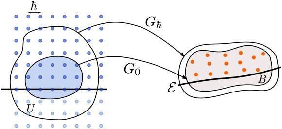
Figure 1: An example of asymptotic half-lattice.

Let $(\hat{J}_{\hbar},\hat{H}_{\hbar})$ be a proper quantum integrable system with joint principal symbol $F=(J,H)$. Let $c=(c_{1},c_{2})$ be a $J$-transversally elliptic critical value of $F$: this is a critical value of elliptic-transverse type of $F$ such that $c_{1}$ is a regular value of $J$ and $c_{2}$ is a non-degenerate critical value of $H$ restricted to the level set $J^{-1}(c_{1})$. Assume that $F^{-1}(c)$ is connected.

By Theorem 7.4, the joint spectrum of $(\hat{J}_{\hbar},\hat{H}_{\hbar})$ near $c$ is an asymptotic half-lattice, whose boundary is the boundary of $F(M)$, with asymptotic chart $G_{\hbar}=G_{0}+\hbar G_{1}+\ldots$ where $G_{0}$ is such that

$$(F\circ\phi^{-1})(\theta_{1},\xi_{1},x_{2},\xi_{2})=G_{0}(\xi_{1},q(x_{2},\xi_{2}))$$

where $(\theta_{1},\xi_{1},x_{2},\xi_{2})$ are coordinates on $T^{*}S^{1}\times T^{*}\mathbb{R}$ endowed with the symplectic form $\omega_{0}=d\xi_{1}\wedge d\theta_{1}+d\xi_{2}\wedge dx_{2}$, $\phi$ is a symplectomorphism from a neighborhood of $F^{-1}(c)$ in $M$ to a neighborhood of the zero section times $T^{*}\mathbb{R}$ in $T^{*}S^{1}\times T^{*}\mathbb{R}$, and $q(x_{2},\xi_{2})=\frac{1}{2}(x_{2}^{2}+\xi_{2}^{2})$. While this statement, which was stated without proof in [27, Theorem 3.36], is sometimes considered “well known” (at least for $\hbar$-pseudodifferential operators), we couldn’t find a proof in the literature; hence we devote Section 7 to filling this gap.

In view of the inverse problem, we will need to label these asymptotic half-lattices. Hence we have to show that they admit a labelling, and to give an algorithm to obtain such a labelling.

Definition 4.9

Let $(\mathcal{L}_{\hbar},\mathcal{I},B)$ be an asymptotic half-lattice with asymptotic chart $(G_{\hbar},U)$. A good labelling of $(\mathcal{L}_{\hbar},\mathcal{I},B)$ is a family of maps $\ell_{\hbar}:\mathcal{L}_{\hbar}\to\mathbb{Z}^{2}$, $\hbar\in\mathcal{I}$, such that for every $\lambda\in\mathcal{L}_{\hbar}$, $\hbar\ell_{\hbar}(\lambda)\in U$ and

$$\forall N\geq 0\qquad\|G_{\hbar}(\hbar\ell_{\hbar}(\lambda))-\lambda\|\leq C_{N}\hbar^{N}$$

where $(C_{N})_{N\geq 0}$ is as in Definition 4.7.

This definition is similar to Definition 4.3, but there is an important difference. Because the labels along the boundary are of the form $(m,0)$, $m\in\mathbb{Z}$, there can only be a drift (see [27, Definition 3.24]) in the horizontal direction. The proof of the following result is similar to the proof of Lemma 3.10 in [27].

Proposition 4.10

Let $(\mathcal{L}_{\hbar},\mathcal{I},B)$ be an asymptotic half-lattice with asymptotic chart $(G_{\hbar},U)$. There exists a good labelling of $(\mathcal{L}_{\hbar},\mathcal{I},B)$ associated with $G_{\hbar}$.

This notion of good labelling is a relevant local notion, but is not sufficient when dealing with global situations. More precisely, it is attached to each component of the boundary $\mathcal{E}$, and cannot be globalised if this boundary is disconnected, see Figure 2.

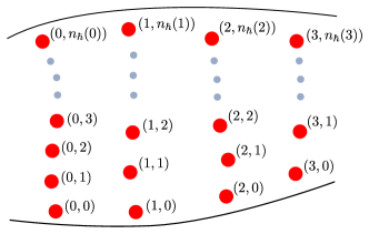
Figure 2: An example of what would be a global labelling of a “global asymptotic lattice”. The labels near the lower boundary correspond to a good labelling, which forces the labels near the upper boundary to be of the form $(m,n_{\hbar}(m))$ with $n_{\hbar}(m)$ of order $\mathscr{O}(1/\hbar)$, so in particular cannot constitute a good labelling.

A good labelling is a special case of linear labelling, the definition of which is similar to the one for asymptotic lattices. However there is a crucial distinction: we need to relax the condition that the labels along the boundary are of the form $(m,0)$, $m\in\mathbb{Z}$. This will be useful when constructing a “global labelling” on the union of an asymptotic lattice and an asymptotic half-lattice, see Lemma 4.26.

Definition 4.11

A linear labelling of an asymptotic half-lattice $(\mathcal{L}_{\hbar},\mathcal{I},B)$ is a family of maps $\bar{\ell}_{\hbar}:\mathcal{L}_{\hbar}\to\mathbb{Z}^{2}$, $h\in\mathcal{I}$ of the form $\bar{\ell}_{\hbar}=A\circ\ell_{\hbar}+\kappa_{\hbar}$ where $\ell_{\hbar}$ is a good labelling, $A\in\mathrm{SL}(2,\mathbb{Z})$ and $(\kappa_{\hbar})_{\hbar\in\mathcal{I}}$ is a family of vectors in $\mathbb{Z}^{2}$.

The following analogue of [27, Proposition 3.19] holds for asymptotic half-lattices.

Lemma 4.12

Let $\bar{\ell}_{\hbar}^{(1)}$ and $\bar{\ell}_{\hbar}^{(2)}$ be two linear labellings for a given asymptotic half-lattice $(\mathcal{L}_{\hbar},\mathcal{I},B)$, then for any open set $\tilde{B}\Subset B$, there exists a unique matrix $A\in\mathrm{SL}(2,\mathbb{Z})$, $\hbar_{0}>0$ and a family $(\kappa_{\hbar})_{\hbar\in\mathcal{I}\cap[0,\hbar_{0}]}$ of vectors in $\mathbb{Z}^{2}$ such that

$$\forall\hbar\in\mathcal{I}\cap[0,\hbar_{0}]\qquad\bar{\ell}_{\hbar}^{(2)}=A\circ\bar{\ell}_{\hbar}^{(1)}+\kappa_{\hbar}\quad\text{ on }\mathcal{L}_{\hbar}\cap\tilde{B}.$$

Proof .  The proof of the analogous result for asymptotic lattices can be adapted by following the same strategy as in the proof of [27, Proposition 3.19]. We construct two affine bases which are adapted to the boundary of the half-lattice by first choosing $\lambda_{0}\in\mathcal{L}_{\hbar}$ so that $\lambda_{0}=G_{\hbar}^{(1)}(n_{1},0)=G_{\hbar}^{(2)}(n_{2},0)$ for some $n_{1},n_{2}\in\mathbb{Z}$, and then by considering the images of the canonical basis of $\mathbb{R}^{2}$ by the two labellings. Then as in the aforementioned proof, the action of $\{-1,0,1\}^{2}$ is transitive, and the analogue of [27, Lemma 3.17], which still holds in this context, allows us to conclude. $\square$

Similarly to the case of usual asymptotic lattices, we define semitoric asymptotic half-lattices by enforcing (11). A consequence of this restriction is that we now have to distinguish between “upper” half-lattices and “lower” half-lattices: the current Definition 4.7 only deals with “upper” half-lattices, while “lower” half-lattices need either replacing $\mathbb{N}$ in that definition by $\mathbb{Z}_{-}$, or requiring $G_{0}$ to be orientation reversing (because switching to the “upper” case amounts to composing by $(x,y)\mapsto(x,-y)$). Since these modifications are rather obvious, for the sake of simplicity we shall discuss only the “upper” case.

Let $(\hat{J}_{\hbar},\hat{H}_{\hbar})$ be a proper semitoric quantum integrable system, and let $c=(c_{1},c_{2})$ be a $J$-transversally elliptic critical value of the underlying integrable system $(J,H)$.

Let $(\Sigma_{\hbar},\mathcal{I},B)$ be the semitoric asymptotic half-lattice formed by the joint spectrum of $(\hat{J}_{\hbar},\hat{H}_{\hbar})$ where $B\subset\mathbb{R}^{2}$ is a neighborhood of $c$. We propose here an algorithm to construct a linear semitoric labelling of this joint spectrum (it would also be interesting to have an algorithm for general asymptotic half-lattices, but in this work we only need the semitoric case). Our algorithm proceeds as follows.

Algorithm 4.13 First, choose an open subset $B_{0}\Subset B$ containing $c$. Then, for any given $\hbar$, follow the steps below.

1. Choose $\mu$, an element of $\Sigma_{\hbar}$ with minimal Euclidean distance to $c$. This element is not necessarily unique.

2. Consider the vertical strip $\mathcal{S}_{0}$ of width $\hbar^{\frac{3}{2}}$ around $\mu$. Let $\lambda_{(0,0)}\in\Sigma_{\hbar}$ be an element with lowest ordinate in that strip. Such an element always exists and, once $\mu$ is chosen (which we assume at this step), $\lambda_{(0,0)}$ is unique if $\hbar$ is small enough.

3. Let $\lambda_{(0,1)}\in\Sigma_{\hbar}\cap\mathcal{S}_{0}$ be the (unique if $\hbar$ is small enough) nearest point to $\lambda_{(0,0)}$ located above $\lambda_{(0,0)}$.

4. Consider now the translated strip $\mathcal{S}_{1}:=\mathcal{S}_{0}+(\hbar,0)$, and choose an element $\lambda_{(1,0)}\in\Sigma_{\hbar}\cap\mathcal{S}_{1}$ with lowest ordinate.

5. Given the triple $(\lambda_{(0,0)},\lambda_{(1,0)},\lambda_{(0,1)})$ (which, for $\hbar$ small enough, will be an affine basis of the asymptotic lattice), we complete the labelling $\lambda_{n,m}$ as in the usual algorithm, but restricting to $m\geq 0$ (thus, we skip steps 10, 11, and 12 of that algorithm).

$\triangle$

Notice that, contrary to the way the general algorithm from [27] works, in the semitoric case it makes more sense to label “vertically”, that is first obtain all the labels $(0,m)$, then all the labels $(1,m)$, and so on. An interesting feature of this algorithm, compared to the algorithm for asymptotic lattices given in [27], is that it does not necessitate a second, correcting, algorithm; thanks to the presence of the boundary, all steps (but the first one) have unique solutions for $\hbar$ small enough.

Proposition 4.14

The algorithm above produces a linear labelling of $(\Sigma_{\hbar},\mathcal{I},B)$ associated with a semitoric asymptotic chart $(G_{\hbar},U)$, that is an asymptotic chart such that the first component $G_{0}^{(1)}$ of $G_{0}=(G_{0}^{(1)},G_{0}^{(2)})$ satisfies ${\rm d}G_{0}^{(1)}={\rm d}\xi_{1}$.

Remark 4.15 This linear labelling, call it $\ell_{\hbar}$, has the nice property that the eigenvalues which are the closest to the line of critical values (which is the boundary of the asymptotic half-lattice $(\Sigma_{\hbar},\mathcal{I},B)$) are labelled as $(n,0)$ with $n\in\mathbb{Z}$. In other words, the only matrix $A$ such that $A\circ\ell_{\hbar}+\kappa_{\hbar}$ is good for some $\kappa_{\hbar}\in\mathbb{Z}^{2}$ (see Definition 4.11) is the identity.   $\triangle$

Proof .  From [27, Proposition 3.35] we know that the joint eigenvalues $\lambda$ in a small neighborhood of $c$ are contained in a union of vertical strips $V_{j}$ given by the equation

$$x=\alpha_{0}+\hbar(j+\alpha_{1}+\mathscr{O}(\lambda-c))+\mathscr{O}(\hbar^{2}),\quad j\in\mathbb{Z},$$

where $\alpha_{0},\alpha_{1}\in\mathbb{R}$ are fixed. Let $V_{j_{0}}$ be the strip containing the point $\mu$ of Step 1 (of course, $j_{0}$ depends on $\hbar$). By [27, Proposition 3.35] the eigenvalues in each strip have, for $\hbar$ small enough, pairwise distinct ordinates, and we may choose the unique lowest one $\lambda_{(0,0)}$ (Step 2, with $\mathcal{S}_{0}\subset V_{j_{0}}$), and the next lowest one $\lambda_{(0,1)}$ (Step 3). Since $\mathcal{S}_{0}+(\hbar,0)\subset V_{j_{0}+1}$, Step 4 similarly defines a unique element $\lambda_{(1,0)}$.

In order to show that the algorithm constructs a linear labelling, we use some details of the proof of [27, Proposition 3.35]. In particular, there exists an asymptotic chart $G_{\hbar}$ for the asymptotic half-lattice $\Sigma_{\hbar}$ such that

$$G_{0}(\xi_{1},\xi_{2})=(\xi_{1}+\alpha_{0},f(\xi_{1},\xi_{2})),\quad\partial_{\xi_{2}}f>0.$$

Let $(\ell_{1},\ell_{2})$ be the good labelling associated with $G_{\hbar}$. The image by $G_{\hbar}$ of $\{\hbar\ell_{1}\}\times\hbar\mathbb{N}$ (restricted to its domain of definition, of course) is contained in one of the strips $V_{j}$, hence, up to a constant $\kappa_{1}(\hbar)\in\mathbb{Z}$, we must have, for each joint eigenvalue $\lambda\in V_{j}$, $\ell_{1}(\lambda)=j+\kappa_{1}(\hbar)$. Since $\partial_{y}f>0$, the joint eigenvalue with label $(\ell_{1},\ell_{2}=0)$ is the lowest of its strip $V_{j}$ and hence must coincide with $\lambda_{(0,0)}$ when $j=j_{0}$, and with $\lambda_{(1,0)}$ when $j=j_{0}+1$. Similarly, the labels of $\lambda_{(0,1)}$ must be $\ell_{1}=j_{0}+\kappa_{1}(\hbar)$, $\ell_{2}=1$. This shows that the triple $(\lambda_{(0,0)},\lambda_{(1,0)},\lambda_{(0,1)})$ is an affine basis of $\Sigma_{\hbar}$, and hence, by parallel transport [27, Proposition 3.16], the labelling $\lambda_{(n,m)}\mapsto(n,m)$ of the algorithm must coincide with the linear labelling

$$\lambda\mapsto(\ell_{1}(\lambda)+\kappa_{1}(\hbar),\ell_{2}(\lambda)).$$

$\square$

Remark 4.16 One could argue that one does not know a priori how to choose a singular value $c$. But $c$ was used to simplify the presentation, and actually its knowledge is not necessary, since the position of a transversally-elliptic value can be obtained up to $\mathscr{O}(\hbar)$ by considering any point in the half-lattice and by finding a point with minimal ordinate in a strip of width $\hbar^{2/3}$ around this point.   $\triangle$

Remark 4.17 There are two other situations that can occur to an integrable system on a four-dimensional manifold.

• The image of the momentum map $F=(J,H)$ could display so-called vertical walls, which correspond to images of $H$-transversally elliptic critical values of $F$. In the case of a semitoric system $(J,H)$, such a vertical wall can only appear at a global minimum or maximum of $J$. It turns out that, although we will have to deal with these vertical walls later on, we will avoid describing the structure of the joint spectrum of $(\hat{J}_{\hbar},\hat{H}_{\hbar})$ near any of their points. Nevertheless, this joint spectrum simply forms a “vertical half-lattice”.

• The image of $F$ may also display “corners” where two lines of transversally elliptic critical values intersect, corresponding to images of singularities of $F$ of elliptic-elliptic type. Again, we will explain below (see Section 5.2) why we do not need to understand the structure of the joint spectrum near such a point. This joint spectrum is neither an asymptotic lattice nor an asymptotic half-lattice, but rather an “asymptotic quarter-lattice” modelled on $\mathbb{N}\times\mathbb{N}$. In the setting of homogeneous pseudodifferential operators, this was the situation studied in [22].

$\triangle$

4.3 Extension of an asymptotic lattice

An important property of asymptotic lattices, which will be key in reconstructing the polygon invariant from the joint spectrum of a quantum semitoric system, is that they behave like flat sheaves.

Lemma 4.18 (restriction of asymptotic lattices)

If $(\mathcal{L}_{\hbar},\mathcal{I},B)$ is an asymptotic lattice, and $\tilde{B}\subset B$ is a simply connected open subset of $B$, then $(\mathcal{L}_{\hbar}\cap\tilde{B},\mathcal{I},\tilde{B})$ is also an asymptotic lattice. Moreover, if $\ell_{\hbar}$ is a good (respectively linear) labelling for $\mathcal{L}_{\hbar}$, then the restriction of ${\ell}_{\hbar}$ to $\tilde{\mathcal{L}}_{\hbar}$ is a good (respectively linear) labelling for $\tilde{\mathcal{L}}_{\hbar}$.

Proof .  We check the various items of Definition 4.1. Item 1 is automatically inherited if we replace $\mathcal{L}_{\hbar}$ by $\tilde{\mathcal{L}}_{\hbar}:=\mathcal{L}_{\hbar}\cap\tilde{B}$. Concerning item 2, we claim that the same chart $G_{\hbar}$ (i.e with domain $\tilde{U}:=U$) is valid: it suffices to check the last property stated below (10). If $\tilde{U}_{0}\subset G_{0}^{-1}(\tilde{B})$ is given, since $\tilde{U}_{0}\subset U_{0}$, by assumption we find a corresponding $\lambda\in\mathcal{L}_{\hbar}$. We also know that $\lambda\in G_{\hbar}(\tilde{U}_{0})+\mathscr{O}(\hbar^{\infty})\subset G_{0}(\tilde{U}_{0})+\mathscr{O}(\hbar)\subset\check{B}+\mathscr{O}(\hbar)$, for some $\check{B}\Subset\tilde{B}$. Hence if $\hbar_{1}$ is small enough, for all $\hbar\leq\hbar_{1}$, $\lambda\in\tilde{B}$. $\square$

We now prove the unique extension property (which is related to the parallel transport of [27]).

Lemma 4.19

Let $(\mathcal{L}_{\hbar},\mathcal{I},B)$ be an asymptotic lattice. Let $\tilde{B}\subset B$ such that $\tilde{B}$ is simply connected. Given any linear labelling $\tilde{\ell}_{\hbar}$ for the asymptotic lattice $(\tilde{\mathcal{L}}_{\hbar}=\mathcal{L}_{\hbar}\cap\tilde{B},\mathcal{I},\tilde{B})$, there exists a linear labelling $\ell_{\hbar}$ for $(\mathcal{L}_{\hbar},\mathcal{I},B)$ which agrees with $\tilde{\ell}_{\hbar}$ on $\mathcal{L}_{\hbar}\cap\check{B}$ for every $\check{B}\Subset\tilde{B}$. Moreover, for any $\hat{B}\Subset B$ containing $\tilde{B}$, the restriction of $\ell_{\hbar}$ to $\mathcal{L}_{\hbar}\cap\hat{B}$ is unique for $\hbar$ small enough. Furthermore, if $\tilde{\ell}_{\hbar}$ is a good labelling, then $\ell_{\hbar}$ is a good labelling as well; in that case, if $G_{\hbar}$ is an asymptotic chart associated with ${\ell}_{\hbar}$, and $\tilde{G}_{\hbar}$ is an asymptotic chart associated with $\tilde{\ell}_{\hbar}$, then $G_{0}^{-1}=\tilde{G}_{0}^{-1}$ on $\tilde{B}$.

Proof .  If $\tilde{B}=B$ or $\tilde{B}=\emptyset$, the statement is trivial, so from now on we assume that $\emptyset\subsetneq\tilde{B}\subsetneq B$. We start with the uniqueness statement. Let $\check{B}\Subset\tilde{B}$ and let $\ell_{\hbar}^{(1)}$, $\ell_{\hbar}^{(2)}$ be two linear labellings agreeing with $\tilde{\ell}_{\hbar}$ on $\mathcal{L}_{\hbar}\cap\check{B}$. Let $\hat{B}\Subset B$ containing $\tilde{B}$; then by [27, Proposition 3.19], there exists a unique matrix $A\in\mathrm{SL}(2,\mathbb{Z})$, $\hbar_{0}>0$ and a unique family $(\kappa_{\hbar})_{\hbar\in\mathcal{I}\cap[0,\hbar_{0}]}$ of vectors in $\mathbb{Z}^{2}$ such that

$$\forall\hbar\in\mathcal{I}\cap[0,\hbar_{0}]\qquad\ell_{\hbar}^{(1)}=A\circ\ell_{\hbar}^{(2)}+\kappa_{\hbar}\quad\text{ on }\mathcal{L}_{\hbar}\cap\hat{B}.$$

Since $\ell_{\hbar}^{(1)}$ and $\ell_{\hbar}^{(2)}$ agree on $\tilde{\mathcal{L}}_{\hbar}$, necessarily $A=\mathrm{Id}$ and $\kappa_{\hbar}=0$ (as long as $\tilde{\mathcal{L}}_{\hbar}$ contains three elements whose images by $\ell_{\hbar}^{(1)}$ form an affine basis of $\mathbb{Z}^{2}$, which is true for $\hbar$ small enough) and $\ell_{\hbar}^{(1)}=\ell_{\hbar}^{(2)}$ on $\mathcal{L}_{\hbar}\cap\hat{B}$.

For the existence part, note that by [27, Lemma 3.10], there exists a linear labelling $\check{\ell}_{\hbar}$ for $(\mathcal{L}_{\hbar},\mathcal{I},B)$. Then the restriction of $\check{\ell}_{\hbar}$ to $\tilde{\mathcal{L}}_{\hbar}$ is a linear labelling for $(\tilde{\mathcal{L}}_{\hbar},\mathcal{I},\tilde{B})$. Hence by [27, Proposition 3.19] again, for any $\check{B}\Subset\tilde{B}$, there exists a unique matrix $C\in\mathrm{SL}(2,\mathbb{Z})$, $\hbar_{1}>0$ and a unique family $(\nu_{\hbar})_{\hbar\in\mathcal{I}\cap[0,\hbar_{1}]}$ of vectors in $\mathbb{Z}^{2}$ such that

$$\forall\hbar\in\mathcal{I}\cap[0,\hbar_{1}]\qquad\check{\ell}_{\hbar}=C\circ\tilde{\ell}_{\hbar}+\nu_{\hbar}\quad\text{ on }\tilde{\mathcal{L}}_{\hbar}\cap\check{B}.$$

Note that by the uniqueness statement, the matrix $C$ does not depend on $\check{B}$ as long as $\check{B}\neq\emptyset$.

Assume that $\tilde{\ell}_{\hbar}$ is a good labelling, and let $\tilde{G}_{\hbar}$ be the associated asymptotic chart. Since $\ell_{\hbar}$ is a linear labelling, there exists a family $(\kappa_{\hbar})$ of vectors in $\mathbb{Z}^{2}$ such that $\ell_{\hbar}+\kappa_{\hbar}$ is a good labelling. Let $\hat{G}_{\hbar}$ be the asymptotic chart associated with this good labelling. It follows from the proof of [27, Proposition 3.19] that $\operatorname{d}\!{\hat{G}_{\hbar}}^{-1}=\operatorname{d}\!{\tilde{G}_{\hbar}}^{-1}+\mathscr{O}(\hbar^{\infty})$ on $\check{B}$. Hence there exists a family $(\nu_{\hbar})_{\hbar\in\mathcal{I}}$ of elements of $\mathbb{R}^{2}$ with an asymptotic expansion in non negative powers of $\hbar$ such that $\hat{G}_{\hbar}^{-1}={\tilde{G}_{\hbar}}^{-1}+\nu_{\hbar}+\mathscr{O}(\hbar^{\infty})$ on $\check{B}$. Since $\ell_{\hbar}=\tilde{\ell}_{\hbar}$ on $\mathcal{L}_{\hbar}\cap\check{B}$, using Equation (10) then yields $\hbar\kappa_{\hbar}=-\nu_{\hbar}+\mathscr{O}(\hbar^{\infty})$. Now, let $G_{\hbar}:\xi\mapsto\hat{G}_{\hbar}(\xi+\nu_{\hbar})$; then $G_{\hbar}$ is an asymptotic chart for $\mathcal{L}_{\hbar}$ and the corresponding good labelling coincides with $\tilde{\ell}_{\hbar}$ on $\mathcal{L}_{\hbar}\cap\check{B}$. $\square$

Lemma 4.20

Let $(\mathcal{L}^{(1)}_{\hbar}\!,\mathcal{I},B_{1})$ and $(\mathcal{L}^{(2)}_{\hbar}\!,\mathcal{I},B_{2})$ be two asymptotic lattices, sharing the same parameter set $\mathcal{I}$. Assume that $B_{1}\cap B_{2}$ is simply connected and non empty, and that

$$\forall\hbar\in\mathcal{I},\quad\mathcal{L}^{(1)}_{\hbar}\cap B_{2}=\mathcal{L}^{(2)}_{\hbar}\cap B_{1}.$$

Then for any simply connected open set $B\Subset B_{1}\cup B_{2}$, $\left((\mathcal{L}^{(1)}_{\hbar}\cup\mathcal{L}^{(2)}_{\hbar})\cap B,\mathcal{I},B\right)$ is an asymptotic lattice.

Proof .  First note that, since $B_{1},B_{2}$ and $B_{1}\cap B_{2}$ are open and connected, they are path connected, and the Seifert-van Kampen theorem implies that $B_{1}\cup B_{2}$ is also simply connected. Since $\mathcal{L}^{(1)}_{\hbar}\cap B_{2}=\mathcal{L}^{(1)}_{\hbar}\cap B_{1}\cap B_{2}$, we may apply Lemma 4.18 to conclude that $(\mathcal{L}^{(1)}_{\hbar}\cap B_{2},\mathcal{I},B_{1}\cap B_{2})$ is an asymptotic lattice. Let $\tilde{\ell}_{\hbar}$ be a good labelling for it. Let $\tilde{B}_{1}\Subset B_{1}$ and $\tilde{B}_{2}\Subset B_{2}$ such that $\bar{B}\subset\tilde{B}=\tilde{B}_{1}\cup\tilde{B}_{2}\Subset B_{1}\cup B_{2}$, and let $W=\tilde{B}_{1}\cap\tilde{B}_{2}$. By Lemma 4.19, we construct a good labelling $\ell^{(1)}_{\hbar}$ for $\mathcal{L}_{\hbar}^{(1)}$ which coincides with $\tilde{\ell}_{\hbar}$ on $\mathcal{L}_{\hbar}^{(1)}\cap W$. Similarly, we construct a good labelling $\ell^{(2)}_{\hbar}$ for $\mathcal{L}_{\hbar}^{(2)}$ which coincides with $\tilde{\ell}_{\hbar}$ on $\mathcal{L}_{\hbar}^{(2)}\cap W$. We may now define the map $\ell_{\hbar}:(\mathcal{L}^{(1)}_{\hbar}\cup\mathcal{L}^{(2)}_{\hbar})\cap\tilde{B}\to\mathbb{Z}$, for all $\hbar\in\mathcal{I}$, by

$$\ell_{\hbar}=\begin{cases}\ell^{(1)}_{\hbar}&\text{ on }\mathcal{L}^{(1)}_{\hbar}\cap\tilde{B}_{1},\\[5.69054pt] \ell^{(2)}_{\hbar}&\text{ on }\mathcal{L}^{(2)}_{\hbar}\cap\tilde{B}_{2}.\end{cases}$$

The labellings $\ell^{(j)}_{\hbar}$, $j=1,2$ are associated with asymptotic charts $G_{\hbar}^{(j)}$, defined on open sets $U_{j}$. By uniqueness of the asymptotic chart associated with a good labelling, $G_{\hbar}^{(1)}=G_{\hbar}^{(2)}+\mathscr{O}(\hbar^{\infty})$ on $V=(G_{0}^{(1)})^{-1}(W)$ (recall that $(G_{0}^{(1)})^{-1}=(G_{0}^{(2)})^{-1}$ on $\tilde{B}_{1}\cap\tilde{B}_{2}$). Hence, $G_{\hbar}^{(1)}$ and $G_{\hbar}^{(2)}$ share the same asymptotic expansion on $V$. We define the family $(G_{\hbar})_{\hbar\in\mathcal{I}}$ on $U:=V_{1}\cup V_{2}$, where $V_{j}:=(G_{0}^{(j)})^{-1}(\tilde{B}_{j})$ by gluing the asymptotic expansions of $G_{\hbar}^{(1)}$ and $G_{\hbar}^{(2)}$ and applying a Borel summation. It remains to prove that the principal term $G_{0}$ is a diffeomorphism into its image $G_{0}(U)=\tilde{B}$. Since it is a local diffeomorphism, we just need to show injectivity. Let $\xi_{1}$, $\xi_{2}\in U$ be such that $G_{0}(\xi_{1})=G_{0}(\xi_{2})$. Notice that $V_{j}\subset U_{j}$, and we know that $G_{0}$ is the restriction of $G_{0}^{(j)}$ on that subset, and hence is injective there. Hence we may assume that $\xi_{j}\in V_{j}$, for $j=1,2$. Hence $G_{0}(\xi_{j})\in\tilde{B}_{j}$; therefore, for $j=1,2$, $G_{0}(\xi_{j})\in\tilde{B}_{1}\cap\tilde{B}_{2}$. Hence $\xi_{j}\in V$, which is contained in, for instance, $V_{1}$, and we can conclude by the injectivity of $G_{0}$ there, that $\xi_{1}=\xi_{2}$.

$\square$

4.4 Extension of an asymptotic half-lattice

We need similar statements for asymptotic half-lattices; but additional difficulties appear. For instance, in the following results, which are the analogues of Lemma 4.18, we must take into account the fact that the restriction of an asymptotic half-lattice can be either an asymptotic lattice or an asymptotic half-lattice, see Figure 3.

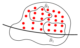
Figure 3: The restriction of this asymptotic half-lattice to $\tilde{B}_{1}$ will be an asymptotic half-lattice, whereas its restriction to $\tilde{B}_{2}$ will be an asymptotic lattice.

Lemma 4.21

Let $(\mathcal{L}_{\hbar},\mathcal{I},B)$ be an asymptotic half-lattice, and let $(\ell_{\hbar})_{\hbar\in\mathcal{I}}$ be a good (respectively linear) labelling for $(\mathcal{L}_{\hbar},\mathcal{I},B)$. Let $\tilde{B}\subset\mathrm{int}(\underline{\mathcal{L}_{\hbar}})$ be any simply connected open set, where $\underline{\mathcal{L}_{\hbar}}$ is the set of accumulation points of $\bigcup_{\hbar\in\mathcal{I}}\mathcal{L}_{\hbar}$ in $B$. Then $(\mathcal{L}_{\hbar}\cap\tilde{B},\mathcal{I},\tilde{B})$ is an asymptotic lattice, and the restriction of $(\ell_{\hbar})_{\hbar\in\mathcal{I}}$ to $\mathcal{L}_{\hbar}\cap\tilde{B}$ is a good (respectively linear) labelling for $(\mathcal{L}_{\hbar}\cap\tilde{B},\mathcal{I},\tilde{B})$.

In the case of the restriction to a subset intersecting the boundary of an asymptotic half-lattice, we need to be a little bit more careful.

Definition 4.22

Let $(\mathcal{L}_{\hbar},\mathcal{I},B)$ be an asymptotic half-lattice. A set $\tilde{B}\subset B$ is called an admissible domain if there exists an asymptotic chart $G_{\hbar}$ such that $\tilde{B}$ is the image by $G_{0}$ of a convex set $K\subset G_{0}^{-1}(B)$ containing a point of the form $(x,0)$, $x\in\mathbb{R}$ (hence this is true for any asymptotic chart).

Note that by definition, $B$ itself is an admissible domain. The proof of the following lemma is similar to the proof of Lemma 4.18.

Lemma 4.23

Let $(\mathcal{L}_{\hbar},\mathcal{I},B)$ be an asymptotic half-lattice, and let $(\ell_{\hbar})_{\hbar\in\mathcal{I}}$ be a good (respectively linear) labelling for $(\mathcal{L}_{\hbar},\mathcal{I},B)$. Let $\tilde{B}\subset B$ be an admissible domain. Then $(\mathcal{L}_{\hbar}\cap\tilde{B},\mathcal{I},\tilde{B})$ is an asymptotic half-lattice, and the restriction of $(\ell_{\hbar})_{\hbar\in\mathcal{I}}$ to $\mathcal{L}_{\hbar}\cap\tilde{B}$ is a good (respectively linear) labelling for $(\mathcal{L}_{\hbar}\cap\tilde{B},\mathcal{I},\tilde{B})$.

Lemma 4.24

Let $(\mathcal{L}_{\hbar},\mathcal{I},B)$ be an asymptotic half-lattice. Let $\tilde{B}\subset B$ be an admissible domain and let $(\tilde{\mathcal{L}}_{\hbar}=\mathcal{L}_{\hbar}\cap\tilde{B},\mathcal{I},\tilde{B})$ be the corresponding asymptotic half-lattice. Given any linear labelling $\tilde{\ell}_{\hbar}$ for $(\tilde{\mathcal{L}}_{\hbar},\mathcal{I},\tilde{B})$, there exists a linear labelling $\ell_{\hbar}$ for $\mathcal{L}_{\hbar}$ which agrees with $\tilde{\ell}_{\hbar}$ on $\tilde{\mathcal{L}}_{\hbar}\cap\check{B}$ for every $\check{B}\Subset\tilde{B}$. Moreover, for any $\hat{B}\Subset B$ containing $\tilde{B}$, the restriction of $\ell_{\hbar}$ to $\mathcal{L}_{\hbar}\cap\hat{B}$ is unique for $\hbar$ small enough. Furthermore, if $\tilde{\ell}_{\hbar}$ is a good labelling, then $\ell_{\hbar}$ is a good labelling as well; in that case, if $G_{\hbar}$ is an asymptotic chart associated with ${\ell}_{\hbar}$, and $\tilde{G}_{\hbar}$ is an asymptotic chart associated with $\tilde{\ell}_{\hbar}$, then $G_{0}^{-1}=\tilde{G}_{0}^{-1}$ on $\tilde{B}\cap\underline{\mathcal{L}_{\hbar}}$.

Proof .  The proof is essentially the same as the proof of Lemma 4.19. When dealing with a half-lattice, one has to use Lemma 4.12 instead of [27, Proposition 3.19]. However, one has to be careful because in that case, given two good labellings which coincide on $\mathcal{L}_{\hbar}\cap\check{B}$ and associated with asymptotic charts $G_{\hbar}$ and $\tilde{G}_{\hbar}$, the equality $\operatorname{d}\!{G}_{\hbar}^{-1}=\operatorname{d}\!{\tilde{G}_{\hbar}}^{-1}+\mathscr{O}(\hbar^{\infty})$ only holds on $\check{B}^{+}=\underline{\mathcal{L}_{\hbar}}\cap\check{B}$. This implies that on $\check{B}$, $G_{\hbar}^{-1}={\tilde{G}_{\hbar}}^{-1}+\nu_{\hbar}+\mathscr{O}(\hbar^{\infty})$ modulo a term which vanishes on $\check{B}^{+}$. But since we use this equality on $\mathcal{L}_{\hbar}$, which is at distance at most $\mathscr{O}(\hbar)$ of $\check{B}^{+}$, the proof still works since the additional term only adds a $\mathscr{O}(\hbar^{\infty})$. Furthermore, there is also a slight difference with the aforementioned proof coming from the fact that if $\ell_{\hbar}$ is a linear labelling, then there exists $A\in\text{SL}(2,\mathbb{Z})$ and $\kappa_{\hbar}\in\mathbb{Z}^{2}$ such that $A\circ\ell_{\hbar}+\kappa_{\hbar}$ is good. But the fact that the above equality only holds on $\check{B}^{+}$ is enough to prove that $A$ is the identity. $\square$

Lemma 4.25

Let $(\mathcal{L}^{(1)}_{\hbar}\!,\mathcal{I},B_{1})$ and $(\mathcal{L}^{(2)}_{\hbar}\!,\mathcal{I},B_{2})$ be two asymptotic half-lattices, sharing the same parameter set $\mathcal{I}$, with respective boundaries $\mathcal{E}_{1}$ and $\mathcal{E}_{2}$ (see Definition 4.8) and asymptotic charts $G_{\hbar}^{(1)}$ and $G_{\hbar}^{(2)}$. Let $\mathcal{L}_{\hbar}=\mathcal{L}^{(1)}_{\hbar}\cup\mathcal{L}^{(2)}_{\hbar}$. Assume that $B_{1}\cap B_{2}$ is simply connected and non empty, that $\mathcal{E}_{1}\cap B_{2}$ is connected and that

$$\forall\hbar\in\mathcal{I},\quad\mathcal{L}^{(1)}_{\hbar}\cap B_{2}=\mathcal{L}^{(2)}_{\hbar}\cap B_{1}.$$

Then $\mathcal{E}_{1}\cap B_{2}=\mathcal{E}_{2}\cap B_{1}$ and for any admissible domain $\tilde{B}\Subset B_{1}\cup B_{2}$, $\left(\mathcal{L}_{\hbar}\cap\tilde{B},\mathcal{I},\tilde{B}\right)$ is an asymptotic half-lattice. Moreover, for $i=1,2$, let $\tilde{B}_{i}\Subset B_{i}$ be an admissible domain. Then there exists a family of maps $(\ell_{\hbar}:\mathcal{L}_{\hbar}\cap(\tilde{B}_{1}\cup\tilde{B}_{2})\to\mathbb{Z}^{2})_{\hbar\in\mathcal{I}}$ such that ${\ell_{\hbar}}_{|\mathcal{L}^{(1)}_{\hbar}\cap\tilde{B}_{1}}$ and ${\ell_{\hbar}}_{|\mathcal{L}^{(2)}_{\hbar}\cap\tilde{B}_{2}}$ are linear labellings for $(\mathcal{L}^{(1)}_{\hbar}\!\cap\tilde{B}_{1},\mathcal{I},\tilde{B}_{1})$ and $(\mathcal{L}^{(2)}_{\hbar}\!\cap\tilde{B}_{2},\mathcal{I},\tilde{B}_{2})$ respectively. Furthermore, $\ell_{\hbar}$ is uniquely defined from its restriction to $\mathcal{L}^{(1)}_{\hbar}\!\cap\tilde{B}_{1}$ or $\mathcal{L}^{(2)}_{\hbar}\!\cap\tilde{B}_{2}$.

Proof .  The proof is similar to the proof of Lemma 4.20. The main differences are the following:

• instead of Lemmas 4.18 and Lemma 4.19, we use Lemmas 4.23 and 4.24,

• as in the proof of Lemma 4.24, the two charts $G_{\hbar}^{(1)}$ and $G_{\hbar}^{(2)}$ will coincide only up to $\mathscr{O}(\hbar^{\infty})$ and a term which vanishes on $\tilde{B}_{1}^{+}\cup\tilde{B}_{2}^{+}$. But then we can still define a common chart $G_{\hbar}$ which coincides with each one of them where it should and which is a diffeomorphism on a neighborhood of $\overline{\tilde{B}_{1}\cup\tilde{B}_{2}}$.

For the last assertion, let $\tilde{B}_{i}\Subset\hat{B}_{i}\Subset B_{i}$ for $i=1,2$. By the first part, there exists a family of maps $({\hat{\ell}}_{\hbar}:\mathcal{L}_{\hbar}\cap(\hat{B}_{1}\cup\hat{B}_{2})\to\mathbb{Z}^{2})_{\hbar\in\mathcal{I}}$ such that the restrictions of $\hat{\ell}_{\hbar}$ to $\mathcal{L}^{(1)}_{\hbar}\cap\hat{B}_{1}$ and $\mathcal{L}^{(2)}_{\hbar}\cap\hat{B}_{2}$ are linear labellings for $(\mathcal{L}^{(1)}_{\hbar}\!\cap\hat{B}_{1},\mathcal{I},\hat{B}_{1})$ and $(\mathcal{L}^{(2)}_{\hbar}\!\cap\hat{B}_{2},\mathcal{I},\hat{B}_{2})$ respectively. By Lemma 4.12, there exists a unique matrix $A\in\mathrm{SL}(2,\mathbb{Z})$, $\hbar_{0}>0$ and a family $(\kappa_{\hbar})_{\hbar\in\mathcal{I}\cap[0,\hbar_{0}]}$ of vectors in $\mathbb{Z}^{2}$ such that

$$\forall\hbar\in\mathcal{I}\cap[0,\hbar_{0}]\qquad\hat{\ell}_{\hbar}=A\circ\ell_{\hbar}+\kappa_{\hbar}\quad\text{ on }\mathcal{L}_{\hbar}^{(1)}\cap\tilde{B_{1}}.$$

So $\check{\ell}_{\hbar}=A^{-1}(\hat{\ell}_{\hbar}-\kappa_{\hbar})$ is a linear labelling on $\mathcal{L}_{\hbar}\cap(\hat{B}_{1}\cup\hat{B}_{2})$ which coincides with $\ell_{\hbar}$ on $\mathcal{L}_{\hbar}^{(1)}\cap\tilde{B_{1}}$. Let $(\ell^{\prime}_{\hbar}:\mathcal{L}_{\hbar}\cap(\tilde{B}_{1}\cup\tilde{B}_{2})\to\mathbb{Z}^{2})_{\hbar\in\mathcal{I}}$ be another family of maps such that ${\ell^{\prime}_{\hbar}}_{|\mathcal{L}^{(1)}_{\hbar}\cap\tilde{B}_{1}}$ and ${\ell^{\prime}_{\hbar}}_{|\mathcal{L}^{(2)}_{\hbar}\cap\tilde{B}_{2}}$ are linear labellings for $(\mathcal{L}^{(1)}_{\hbar}\!\cap\tilde{B}_{1},\mathcal{I},\tilde{B}_{1})$ and $(\mathcal{L}^{(2)}_{\hbar}\!\cap\tilde{B}_{2},\mathcal{I},\tilde{B}_{2})$ respectively, and such that the restrictions of $\ell_{\hbar}$ and $\ell^{\prime}_{\hbar}$ to $\mathcal{L}^{(1)}_{\hbar}\cap\tilde{B}_{1}$ coincide. Let $\hat{\ell}^{\prime}_{\hbar}$ be its extension to $\mathcal{L}_{\hbar}\cap(\hat{B}_{1}\cup\hat{B}_{2})$ as before. By applying Lemma 4.12 again, there exists a unique matrix $A\in\mathrm{SL}(2,\mathbb{Z})$, $\hbar_{1}>0$ and a family $(\kappa_{\hbar})_{\hbar\in\mathcal{I}\cap[0,\hbar_{1}]}$ of vectors in $\mathbb{Z}^{2}$ such that

$$\forall\hbar\in\mathcal{I}\cap[0,\hbar_{1}]\qquad\hat{\ell}^{\prime}_{\hbar}=A\circ\hat{\ell}_{\hbar}+\kappa_{\hbar}\quad\text{ on }\mathcal{L}_{\hbar}^{(2)}\cap\tilde{B_{2}}.$$

But since $\hat{\ell}^{\prime}_{\hbar}$ and $\hat{\ell}_{\hbar}$ coincide on $\mathcal{L}_{\hbar}^{(2)}\cap\tilde{B_{1}}\cap\tilde{B_{2}}$ by construction, we obtain that $\kappa_{\hbar}=0$ and $A=I$. So $\hat{\ell}^{\prime}_{\hbar}=\hat{\ell}_{\hbar}$ on $\mathcal{L}_{\hbar}\cap(\tilde{B}_{1}\cup\tilde{B}_{2})$. $\square$

In fact, we can also consider the union of one asymptotic lattice and one asymptotic half-lattice.

Lemma 4.26

Let $(\mathcal{L}^{(1)}_{\hbar}\!,\mathcal{I},B_{1})$ be an asymptotic half-lattice and $(\mathcal{L}^{(2)}_{\hbar}\!,\mathcal{I},B_{2})$ be an asymptotic lattice, sharing the same parameter set $\mathcal{I}$, with respective asymptotic charts $G_{\hbar}^{(1)}$ and $G_{\hbar}^{(2)}$. Let $\mathcal{L}_{\hbar}=\mathcal{L}^{(1)}_{\hbar}\cup\mathcal{L}^{(2)}_{\hbar}$. Assume that $B_{1}\cap B_{2}$ is simply connected and non empty, and that

$$\forall\hbar\in\mathcal{I},\quad\mathcal{L}^{(1)}_{\hbar}\cap B_{2}=\mathcal{L}^{(2)}_{\hbar}\cap B_{1}.$$

Let $\tilde{B}_{1}\Subset B_{1}$ be an admissible domain and let $\tilde{B}_{2}\Subset B_{2}$ be simply connected. Then there exists a family of maps $(\ell_{\hbar}:\mathcal{L}_{\hbar}\cap(\tilde{B}_{1}\cup\tilde{B}_{2})\to\mathbb{Z}^{2})_{\hbar\in\mathcal{I}}$ such that ${\ell_{\hbar}}_{|\mathcal{L}^{(1)}_{\hbar}\cap\tilde{B}_{1}}$ and ${\ell_{\hbar}}_{|\mathcal{L}^{(2)}_{\hbar}\cap\tilde{B}_{2}}$ are linear labellings for $(\mathcal{L}^{(1)}_{\hbar}\!\cap\tilde{B}_{1},\mathcal{I},\tilde{B}_{1})$ and $(\mathcal{L}^{(2)}_{\hbar}\!\cap\tilde{B}_{2},\mathcal{I},\tilde{B}_{2})$ respectively. Moreover, $\ell_{\hbar}$ is uniquely defined from its restriction to $\mathcal{L}^{(1)}_{\hbar}\!\cap\tilde{B}_{1}$ or $\mathcal{L}^{(2)}_{\hbar}\!\cap\tilde{B}_{2}$. Furthermore, if $\tilde{B}\Subset B_{1}\cup B_{2}$ is admissible, then $\left(\mathcal{L}_{\hbar}\cap\tilde{B},\mathcal{I},\tilde{B}\right)$ is an asymptotic half-lattice.

Proof .  The proof is similar to the proof of Lemma 4.25, taking into account the definition of linear labelling for an asymptotic half-lattice (Definition 4.11), which allows the composition with an arbitrary element of $\text{SL}(2,\mathbb{Z})$. $\square$

4.5 Global labellings

Using the previous results, we can construct a “global labelling” for the union of several asymptotic lattices and asymptotic half-lattices, under suitable assumptions.

When working with a union of asymptotic lattices (respectively a union of half-lattices sharing a connected boundary), we can directly apply Lemmas 4.20 and 4.25 to obtain the following.

Corollary 4.27

Let $B_{1},\ldots,B_{p}\subset\mathbb{R}^{2}$ be simply connected open sets such that for every $i\in\{1,\ldots,p\}$, $(\mathcal{L}^{(i)}_{\hbar}\!,\mathcal{I},B_{i})$ is an asymptotic lattice. Assume that $B=\bigcup_{i=1}^{q}B_{i}$ is simply connected and that for every $i,j$ such that $B_{i}\cap B_{j}\neq\emptyset$:

• $B_{i}\cap B_{j}$ is simply connected,

• $\forall\hbar\in\mathcal{I}$, $\mathcal{L}^{(i)}_{\hbar}\cap B_{j}=\mathcal{L}^{(j)}_{\hbar}\cap B_{i}$.

Let $\mathcal{L}_{\hbar}:=\bigcup_{i=1}^{p}\mathcal{L}^{(i)}_{\hbar}$. Then for every simply connected set $\tilde{B}\Subset B$, $(\mathcal{L}_{\hbar}\cap\tilde{B},\mathcal{I},\tilde{B})$ is an asymptotic lattice.

Corollary 4.28

Let $B_{1},\ldots,B_{p}\subset\mathbb{R}^{2}$ be simply connected open sets such that for every $i\in\{1,\ldots,p\}$, $(\mathcal{L}^{(i)}_{\hbar}\!,\mathcal{I},B_{i})$ is an asymptotic half-lattice. Assume that $\bigcup_{i=1}^{q}B_{i}$ is simply connected and that for every $i,j$ such that $B_{i}\cap B_{j}\neq\emptyset$:

• $B_{i}\cap B_{j}$ is simply connected,

• $\forall\hbar\in\mathcal{I}$, $\mathcal{L}^{(i)}_{\hbar}\cap B_{j}=\mathcal{L}^{(j)}_{\hbar}\cap B_{i}$,

• $B_{i}\cap B_{j}$ is admissible and $\mathcal{E}_{i}\cap B_{j}$ is connected (recall that $\mathcal{E}_{i}$ stands for the boundary of $(\mathcal{L}^{(i)}_{\hbar}\!,\mathcal{I},B_{i})$).

Let $\mathcal{L}_{\hbar}:=\bigcup_{i=1}^{q}\mathcal{L}^{(i)}_{\hbar}$. Then for every admissible $\tilde{B}\Subset B$, $(\mathcal{L}_{\hbar}\cap\tilde{B},\mathcal{I},\tilde{B})$ is an asymptotic half-lattice.

In particular, when working with the joint spectrum $\Sigma_{\hbar}$ of a proper quantum integrable system, the first of these results implies that we can obtain good quantum numbers for the intersection of $\Sigma_{\hbar}$ with any simply connected subset of the set of regular values of the momentum map. Similarly, the second result implies that we can label this joint spectrum along a line of transversally-elliptic values, as long as we do not encounter any elliptic-elliptic value.

Remark 4.29 It follows from Lemma 4.25 that the union of the boundaries of the asymptotic half-lattices in Corollary 4.28 is a one-dimensional manifold $\mathcal{E}$. This corollary implies the interesting topological fact that no component of $\mathcal{E}$ is closed. Indeed, $\Phi(\mathcal{E})$ is an affine line with a natural orientation coming from the fact that the points of the union of the half-lattices always stand on the same side of this line. This is the quantum version of a result that also holds classically, see for instance [93, Theorem 3.4].   $\triangle$

Now, if we want to obtain a global labelling for a union of both asymptotic lattices and half-lattices, we need to work a little bit more. This will be crucial in the next section since we will want to produce good quantum numbers near both regular and transversally elliptic values.

Theorem 4.30

Let $B_{1},\ldots,B_{p},B_{p+1},\ldots,B_{q}\subset\mathbb{R}^{2}$ be simply connected open sets such that for every $i\in\{1,\ldots,p\}$, $(\mathcal{L}^{(i)}_{\hbar}\!,\mathcal{I},B_{i})$ is an asymptotic lattice and for every $i\in\{p+1,\ldots,q\}$, $(\mathcal{L}^{(i)}_{\hbar}\!,\mathcal{I},B_{i})$ is an asymptotic half-lattice. Assume that $\bigcup_{i=1}^{q}B_{i}$ is simply connected and that for every $i,j$ such that $B_{i}\cap B_{j}\neq\emptyset$:

• $B_{i}\cap B_{j}$ is simply connected,

• $\forall\hbar\in\mathcal{I}$, $\mathcal{L}^{(i)}_{\hbar}\cap B_{j}=\mathcal{L}^{(j)}_{\hbar}\cap B_{i}$,

• if $i,j\in\{p+1,\ldots,q\}$, $B_{i}\cap B_{j}$ is admissible and $\mathcal{E}_{i}\cap B_{j}$ is connected.

Let $(\tilde{B}_{i})_{1\leq i\leq q}$ be a family of open sets satisfying the same assumptions as the $B_{i}$ and such that for every $i$, $\tilde{B}_{i}\Subset B_{i}$ and for every $i\in\{p+1,\ldots,q\}$, $\tilde{B}_{i}$ is admissible. Let $\mathcal{L}_{\hbar}:=\bigcup_{i=1}^{q}\mathcal{L}^{(i)}_{\hbar}$. Then there exists a family of maps $\ell_{\hbar}:\mathcal{L}_{\hbar}\cap\bigcup_{i=1}^{q}\tilde{B}_{i}\to\mathbb{Z}^{2}$ such that for every $i\in\{1,\ldots,q\}$, ${\ell_{\hbar}}_{|\mathcal{L}^{(i)}_{\hbar}\cap\tilde{B}_{i}}$ is a linear labelling. Moreover, $\ell_{\hbar}$ is uniquely defined by its restriction to any of the $\mathcal{L}^{(i)}_{\hbar}\cap\tilde{B}_{i}$. Furthermore, there exist a smooth function $\Phi$ from a neighborhood of $\overline{\bigcup_{i=1}^{q}B_{i}}$ to $\mathbb{R}^{2}$, a family $(\nu_{\hbar})$ of vectors in $\mathbb{Z}^{2}$ and a constant $K>0$ such that for every $\hbar$ small enough and for every $\lambda\in\mathcal{L}_{\hbar}\cap\bigcup_{i=1}^{q}\tilde{B}_{i}$,

$$\|\Phi(\lambda)-\hbar\ell_{\hbar}(\lambda)-\nu_{\hbar}\|\leq K\hbar.$$

Proof .  Let $\ell_{\hbar}^{(1)},\ldots,\ell_{\hbar}^{(q)}$ be linear labellings for $(\mathcal{L}^{(1)}_{\hbar}\!,\mathcal{I},B_{1}),\ldots,(\mathcal{L}^{(q)}_{\hbar}\!,\mathcal{I},B_{q})$. For every pair $(i,j)$ such that $\tilde{B}_{i}\cap\tilde{B}_{j}\neq\emptyset$, $\mathcal{L}_{\hbar}\cap\tilde{B}_{i}\cap\tilde{B}_{j}$ is an asymptotic lattice or half-lattice thanks to Lemmas 4.18, 4.21 and 4.23, so by [27, Proposition 3.19] and Lemma 4.12, there exists a unique matrix $A_{ji}\in\mathrm{SL}(2,\mathbb{Z})$, $\hbar_{ji}>0$ and a family $(\kappa_{\hbar}^{(ji)})_{\hbar\in\mathcal{I}\cap[0,\hbar_{ji}]}$ of vectors in $\mathbb{Z}^{2}$ such that

$$\forall\hbar\in\mathcal{I}\cap[0,\hbar_{0}]\qquad\ell_{\hbar}^{(j)}=A_{ji}\circ\ell_{\hbar}^{(i)}+\kappa_{\hbar}^{(ji)}\quad\text{ on }\mathcal{L}_{\hbar}^{(i)}\cap\tilde{B}_{j}.$$

Let $\hbar_{0}=\min_{i,j}\hbar_{ji}>0$. Then we obtain a family of affine maps $\phi_{ji}=A_{ji}\cdot+\kappa_{\hbar}^{(ji)}$ defined for $\hbar\in\mathcal{I}\cap(0,\hbar_{0}]$, which is in fact a cocycle: whenever $\tilde{B}_{i}\cap\tilde{B}_{j}\cap\tilde{B}_{k}\neq\emptyset$, $\phi_{ij}\circ\phi_{jk}\circ\phi_{ki}=I$. Let $c_{0}\in\bigcup_{i=1}^{q}\tilde{B}_{i}$. For every $c\in\bigcup_{i=1}^{q}\tilde{B}_{i}$, we construct the map $\ell_{\hbar}$ in a neighborhood of $c$ as follows. Let $\gamma$ be a continuous path from $c_{0}$ to $c$. Let $\tilde{B}_{i_{0}},\ldots,\tilde{B}_{i_{n}}$ be a chain from $c_{0}$ to $c$ covering $\gamma$, that is $\tilde{B}_{i_{p}}\cap\tilde{B}_{i_{p+1}}\neq\emptyset$ for every $p$, $c_{0}\in\tilde{B}_{i_{0}}$ and $c\in\tilde{B}_{i_{n}}$. Then we construct $\ell_{\hbar}$ near $c$ by setting $\ell_{\hbar}=\phi_{i_{0}i_{1}}\circ\ldots\circ\phi_{i_{n-1}i_{n}}\circ\ell_{\hbar}^{(n)}$. Then by a standard argument (for instance by induction on $n$) using the cocycle condition, $\ell_{\hbar}$ does not depend on the choice of such a chain. The same argument implies that $\ell_{\hbar}$ does not depend on the choice of $\gamma$ up to homotopy with fixed endpoints. Since $\bigcup_{i=1}^{q}\tilde{B}_{i}$ is simply connected, $\ell_{\hbar}$ is well-defined.

Now, let $j\in\{1,\ldots,q\}$; then ${\ell_{\hbar}}_{|\tilde{B}_{j}\cap\mathcal{L}^{(j)}_{\hbar}}$ is a linear labelling, so there exist a matrix $A_{j}\in\text{SL}(2,\mathbb{Z})$ and a vector $\kappa_{\hbar}^{(j)}$ such that $\tilde{\ell}_{\hbar}^{(j)}:=A_{j}\circ\ell_{\hbar}+\kappa_{\hbar}^{(j)}$ is a good labelling for $\tilde{B}_{j}\cap\mathcal{L}^{(j)}_{\hbar}$ (recall Definition 4.11 for half-lattices). Let $G_{\hbar}^{(j)}$ be a corresponding asymptotic chart, and let $U_{j}=(G_{0}^{(j)})^{-1}(\tilde{B}_{j})\subset(G_{0}^{(j)})^{-1}(B_{j})$. Let $\hbar_{0}>0$ and for every $j\in\{1,\ldots,q\}$, let $C_{j},M_{j},L_{j}$ be the constants such that $\forall\hbar\in\mathcal{I}\cap[0,h_{0}]$

$$\begin{cases}\forall\lambda_{\hbar}\in\mathcal{L}_{\hbar}^{(j)}\cap\tilde{B}_{j}\qquad\|G_{\hbar}^{(j)}(\hbar\tilde{\ell}_{\hbar}^{(j)}(\lambda_{\hbar}))-\lambda_{\hbar}\|\leq C_{j}\hbar,\\ \sup_{U_{j}}\|G_{\hbar}^{(j)}-G_{0}^{(j)}\|\leq M_{j}\hbar,\end{cases}$$

and let $D_{j}=\sup_{U_{j}}\|\operatorname{d}\!{(}G_{0}^{(j)})^{-1}\|$. The existence of $C_{j}$ comes from the definitions of asymptotic lattices and half-lattices, and the existence of $M_{j}$ comes from item $2.$ in [27, Lemma 3.7] for the case of asymptotic lattices; this still holds for asymptotic half-lattices, since this is a direct consequence of the asymptotic expansion (9) which also holds for asymptotic half-lattices, see Equation (12). Finally, let $C=\max_{j\in\{1,\ldots,q\}}C_{j}$, $M=\max_{j\in\{1,\ldots,q\}}M_{j}$, $D=\max_{j\in\{1,\ldots,q\}}D_{j}$ and $\alpha=\max_{j}\|A_{j}^{-1}\|$. Then for $\lambda_{\hbar}\in\mathcal{L}_{\hbar}^{(j)}\cap\tilde{B}_{j}$

$$\begin{split}\left\|G_{0}^{(j)}(\hbar\tilde{\ell}_{\hbar}^{(j)}(\lambda_{\hbar}))-\lambda_{\hbar}\right\|&\leq\left\|G_{0}^{(j)}(\hbar\tilde{\ell}_{\hbar}^{(j)}(\lambda_{\hbar}))-G_{\hbar}^{(j)}(\hbar\tilde{\ell}_{\hbar}^{(j)}(\lambda_{\hbar}))\right\|+\left\|G_{\hbar}^{(j)}(\hbar\tilde{\ell}_{\hbar}^{(j)}(\lambda_{\hbar}))-\lambda_{\hbar}\right\|\\ &\leq(M+C)\hbar.\end{split}$$

This implies that

$$\left\|\hbar\tilde{\ell}_{\hbar}^{(j)}(\lambda_{\hbar})-(G_{0}^{(j)})^{-1}(\lambda_{\hbar})\right\|=\left\|(G_{0}^{(j)})^{-1}(G_{0}^{(j)}(\hbar\tilde{\ell}_{\hbar}^{(j)}(\lambda_{\hbar}))-(G_{0}^{(j)})^{-1}(\lambda_{\hbar})\right\|\leq D(M+C)\hbar.$$

So if we set $\Phi_{j}:=(G_{0}^{(j)}\circ A_{j})^{-1}$, we finally obtain that

$$\left\|\hbar\ell_{\hbar}(\lambda_{\hbar})+\hbar A_{j}^{-1}\kappa_{\hbar}^{(j)}-\Phi_{j}(\lambda_{\hbar})\right\|\leq\alpha D(M+C)\hbar.$$ (14)

Now, assume that $\tilde{B}_{i}\cap\tilde{B}_{j}\neq\emptyset$. Then (14) implies that for every $\lambda_{\hbar}\in\mathcal{L}_{\hbar}^{(j)}\cap\tilde{B}_{i}=\mathcal{L}_{\hbar}^{(i)}\cap\tilde{B}_{j}$,

$$\left\|\hbar A_{j}^{-1}\kappa_{\hbar}^{(j)}-\hbar A_{i}^{-1}\kappa_{\hbar}^{(i)}+\Phi_{i}(\lambda_{\hbar})-\Phi_{j}(\lambda_{\hbar})\right\|\leq 2\alpha D(M+C)\hbar.$$ (15)

Let $c\in\tilde{B}_{i}\cap\tilde{B}_{j}$. From [27, Lemma 3.14] and its proof (which works similarly for half-lattices), there exists $\hbar_{1}\leq\hbar_{0}$ and a family $(\lambda_{\hbar})_{\hbar\in\mathcal{I}\cap[0,\hbar_{1}]}$ such that $\forall\hbar\in\mathcal{I}\cap[0,\hbar_{1}]$, $\lambda_{\hbar}\in\tilde{B}_{i}\cap\tilde{B}_{j}$ and $\lambda_{\hbar}\underset{\hbar\to 0}{\longrightarrow}c$. Then the above equation implies that $\hbar A_{j}^{-1}\kappa_{\hbar}^{(j)}-\hbar A_{i}^{-1}\kappa_{\hbar}^{(i)}$ has a limit when $\hbar\to 0$, and that $\Phi_{i}(c)-\Phi_{j}(c)$ does not depend on $c$. Hence ${\operatorname{d}\!{\Phi}_{i}}_{|\tilde{B}_{i}\cap\tilde{B}_{j}}={\operatorname{d}\!{\Phi}_{j}}_{|\tilde{B}_{i}\cap\tilde{B}_{j}}$, so by connectedness there exists a global $\Phi$ such that ${\operatorname{d}\!{\Phi}}_{|\tilde{B}_{j}}={\operatorname{d}\!{\Phi}_{j}}_{|\tilde{B}_{j}}$ for every $j$.

So let $v_{j}\in\mathbb{R}^{2}$ be the constant such that $\Phi(c)=\Phi_{j}(c)+v_{j}$ for every $c\in\tilde{B}_{j}$, and set $\nu_{\hbar}^{(j)}:=\hbar A_{j}^{-1}\kappa_{\hbar}^{(j)}+v_{j}$. Equation (15) yields

$$\left\|\nu_{\hbar}^{(j)}-\nu_{\hbar}^{(i)}\right\|\leq\alpha D(M+C)\hbar$$

whenever $\tilde{B}_{i}\cap\tilde{B}_{j}\neq\emptyset$. So by considering chains of $\tilde{B}_{m}$, we obtain that for any $i,j$, $\|\nu_{\hbar}^{(j)}-\nu_{\hbar}^{(i)}\|\leq q\alpha D(M+C)\hbar$. Thus, if $\nu_{\hbar}:=\frac{1}{q}\sum_{i=1}^{q}\nu_{\hbar}^{(i)}$, we have $\|\nu_{\hbar}-\nu_{\hbar}^{(j)}\|\leq q\alpha D(M+C)\hbar$ for every $j$, and Equation (14) implies that for every $\lambda_{\hbar}\in\mathcal{L}_{\hbar}\cap\bigcup_{i=1}^{q}\tilde{B}_{i}$,

$$\left\|\hbar\ell_{\hbar}(\lambda_{\hbar})+\nu_{\hbar}-\Phi(\lambda_{\hbar})\right\|\leq(q+1)\alpha D(M+C)\hbar.$$

$\square$

Remark 4.31 Depending on the topology of the union in the previous proposition, one may be able to find a family of vectors $\kappa_{\hbar}\in\mathbb{Z}^{2}$ such that $\ell_{\hbar}+\kappa_{\hbar}$ is a “good global labelling” in the sense that its restriction to every $\tilde{B}_{i}$ is a good labelling. This is for instance the case when the boundary attached to the half-lattices is connected. However, as explained in the discussion preceding Figure 2, there is no chance to obtain the same result in all generality.   $\triangle$

Remark 4.32 In view of the above proposition and its proof, it suffices to be able to produce any linear labelling on each of the asymptotic lattices and half-lattices to be able to construct the global labelling $\ell_{\hbar}$. Indeed once such labellings are given, the affine maps relating them and coming from [27, Proposition 3.19] and Lemma 4.12 can be explicitly recovered. In the case where these lattices are of the form $\mathcal{L}^{(i)}_{\hbar}=\Sigma_{\hbar}\cap B_{i}$ where $\Sigma_{\hbar}$ is the joint spectrum of a proper quantum semitoric system and $B_{i}$ is a small neighborhood of a regular or $J$-transversally elliptic value, the algorithms described at the end of Sections 4.1 and 4.2 allow to obtain such linear labellings $\ell_{\hbar}^{(i)}$, hence $\ell_{\hbar}$ can be fully constructed algorithmically.

Note that, on the contrary, this proof does not give any procedure to recover the family of vectors $\nu_{\hbar}$. But as we will see in the next section, knowing the value of $\nu_{\hbar}$ is not necessary for our inverse spectral result for semitoric systems.   $\triangle$

5 Recovering the twisting index from the joint spectrum

In this section we are given a proper quantum semitoric system $(\hat{J}_{\hbar},\hat{H}_{\hbar})$, and we explain how to use the results of the previous section to recover the twisting index invariant from its joint spectrum. Since the twisting index is the data of the polygon invariant decorated with the corresponding twisting numbers for each focus-focus value, we proceed in two steps: the first step is to recover the invariants $\sigma_{1}^{\textup{p}}(0)$ associated with the focus-focus values (see Section 2.4), and the second step is to recover the polygonal invariant and all the attached twisting numbers.

5.1 Recovering $\sigma_{1}(0)$

Theorem 5.1

From the $\hbar$-family of joint spectra $\Sigma_{\hbar}$ of a proper quantum semitoric system in a neighborhood of a focus-focus critical value $c_{0}=0$, one can recover, in a constructive way, the symplectic invariant $[S_{1,0}]$ (see Section 2.5). More precisely, given a semitoric labelling $\lambda_{j,\ell}(\hbar)$ on a small ball near $0$ containing only regular values of $F$, associated with an action variable $L$, one can recover, in a constructive way, the quantity $\sigma_{1}(0)$ associated with $L$ (see Lemma 2.7).

This theorem is the key result used in the proof of Theorem 5.13 to recover the twisting numbers.

Because a uniform description of the joint spectrum in a neighborhood of the focus-focus value exists only for pseudodifferential operators [91], we shall here prove this theorem by a simpler, albeit less efficient (from a numerical viewpoint), approach, which consists in considering regular values $c$ close to $0$, before letting them tend to the origin.

Thus, let $c$ be a regular value of $F$ and let $B\subset\mathbb{R}^{2}$ be an open ball containing $c$, small enough to contain only regular values of $F$. Here we assume that $c$ is sufficiently close to $0$ so that $B$ is contained in the simply connected set $U$ contained in a punctured neighborhood of $0$ defined in Section 2.4. Let

$$(\lambda_{j,\ell}(\hbar))_{j,\ell}=(J_{j,\ell}(\hbar),E_{j,\ell}(\hbar)),$$ (16)

where $(j,\ell)\in\mathbb{Z}^{2}$, be a good labelling of $\mathcal{L}_{\hbar}\cap B$ (see Remark 4.3), associated with a semitoric asymptotic chart $G_{\hbar}:\tilde{U}\to\mathbb{R}^{2}$, where $\tilde{U}\subset\mathbb{R}^{2}$ is some bounded open set; such a labelling is given by [27, Proposition 3.45] and is constructed from $\mathcal{L}_{\hbar}$ thanks to an explicit algorithm, see the discussion at the end of Section 4.1. By definition, $G_{\hbar}$ has an asymptotic expansion of the form

$$G_{\hbar}=G_{0}+\hbar G_{1}+\hbar^{2}G_{2}+\ldots$$

in the $C^{\infty}$ topology, where $G_{0}^{-1}$ is an action diffeomorphism (see Section 2.1); there exists a choice of action variables $(J,L)$ defined near $F^{-1}(c)$ such that

$$F=(J,H)=G_{0}(J,L).$$ (17)

Lemma 5.2

Let $j,\ell$ be $\hbar$-dependent integers such that the joint eigenvalues $\lambda_{j,\ell}$, $\lambda_{j+1,\ell}$ and $\lambda_{j,\ell+1}$ are well-defined in an $\mathscr{O}(\hbar)$-neighborhood of $c$. We have:

1. $\displaystyle\frac{E_{j,\ell}-E_{j+1,\ell}}{\hbar}=\frac{a_{1}(c)}{a_{2}(c)}+\mathscr{O}_{c}(\hbar)$,

2. $\displaystyle\frac{\hbar}{E_{j,\ell+1}-E_{j,\ell}}=a_{2}(c)+\mathscr{O}_{c}(\hbar)$,

where $a_{1},a_{2}$ are the functions that appear in the decomposition (5) of $L$, and $E_{j,\ell}$ is the second component of $\lambda_{j,\ell}$, see (16).

Proof .  From (17), we have that $(J,L)=G_{0}^{-1}(J,H)$. It follows (with a slight abuse of notation) that

$$\begin{pmatrix}\mathcal{X}_{J}\\ \mathcal{X}_{L}\end{pmatrix}=\operatorname{d}\!{G}_{0}^{-1}(J,H)\begin{pmatrix}\mathcal{X}_{J}\\ \mathcal{X}_{H}\end{pmatrix};$$

comparing this with Equation (5) yields, with $\xi_{0}=G_{0}^{-1}(c)$,

$$\operatorname{d}\!{G}_{0}^{-1}(c)=\begin{pmatrix}1&0\\ a_{1}(c)&a_{2}(c)\end{pmatrix},\quad\operatorname{d}\!{G}_{0}(\xi_{0})=\begin{pmatrix}1&0\\ -\frac{a_{1}(c)}{a_{2}(c)}&\frac{1}{a_{2}(c)}\end{pmatrix}.$$

By definition of $G_{\hbar}$, we have that

$$\lambda_{j,\ell}=G_{\hbar}(\hbar j,\hbar\ell)+\mathscr{O}(\hbar^{\infty})=G_{0}(\hbar j,\hbar\ell)+\hbar G_{1}(\hbar j,\hbar\ell)+\mathscr{O}(\hbar^{2}),$$

where the $\mathscr{O}(\hbar^{2})$ is uniform assuming $(\hbar j,\hbar\ell)$ stays in a compact set. On the other hand, we have by assumption $\lambda_{j,\ell}-c=\mathscr{O}(\hbar)$, hence by invertibility of $G_{\hbar}$ [27, Lemma 3.7], we obtain $(\hbar j,\hbar\ell)=\mathscr{O}(\hbar)$ as well. Therefore, Taylor’s formula gives

$$\begin{cases}\lambda_{j,\ell}-\lambda_{j+1,\ell}=-\hbar\operatorname{d}\!{G}_{0}(\hbar j,\hbar\ell)\cdot\vec{z}_{1}+\mathscr{O}(\hbar^{2})\\ \lambda_{j,\ell+1}-\lambda_{j,\ell}=\hbar\operatorname{d}\!{G}_{0}(\hbar j,\hbar\ell)\cdot\vec{z}_{2}+\mathscr{O}(\hbar^{2})\end{cases}$$

where $\vec{z}_{1}:=(\begin{smallmatrix}1\\ 0\end{smallmatrix})$, $\textstyle\vec{z}_{2}:=(\begin{smallmatrix}0\\ 1\end{smallmatrix})$. Since $\lambda_{j,\ell}=c+\mathscr{O}(\hbar)$, we have $(\hbar j,\hbar\ell)=\xi_{0}+\mathscr{O}(\hbar)$ where $\xi_{0}=G_{0}^{-1}(c)$. Hence

$$\lambda_{j,\ell}-\lambda_{j+1,\ell}=-\hbar\ \operatorname{d}\!{G}_{0}(\xi_{0})\cdot\vec{z}_{1}+\mathscr{O}(\hbar^{2}),$$

so finally, taking the second component,

$$\frac{E_{j,\ell}-E_{j+1,\ell}}{\hbar}=\frac{a_{1}(c)}{a_{2}(c)}+\mathscr{O}(\hbar).$$

Similarly,

$$\frac{E_{j,\ell+1}-E_{j,\ell}}{\hbar}=\operatorname{d}\!{G}_{0}(\xi_{0})\cdot\vec{z}_{2}+\mathscr{O}(\hbar^{2})=\frac{1}{a_{2}(c)}+\mathscr{O}(\hbar).$$

$\square$

Remark 5.3 By multiplying the two lines of Lemma 5.2, we obtain

$$\frac{E_{j,\ell}-E_{j+1,\ell}}{E_{j,\ell+1}-E_{j,\ell}}=a_{1}(c)+\mathscr{O}_{c}(\hbar)$$

and $a_{1}$ is precisely the rotation number of $H$ with respect to $(J,L)$, which recovers a result of [27].   $\triangle$

Lemma 5.4

In order to compute $\sigma_{1}(0)$ (see Lemma 2.7), the radial curve $\gamma_{r}$ (see Definition 2.6) can be replaced by any curve that is tangent to $\gamma_{r}$ at the origin.

Proof .  Let $\gamma$ be any curve that is tangent to $\gamma_{r}$ at the origin; then $\gamma$ is also the graph of a smooth function $\psi$. Keeping the notation introduced in the proof of Lemma 2.7, and letting $w_{\psi}(x):=x+if_{r}(x,\psi(x))$, we have that

$$x\mapsto\sigma_{1}(x,\psi(x))=\tau_{1}(x,\psi(x))+\frac{1}{2\pi}\Im(\log(w_{\psi}(x)))$$

is smooth at $x=0$, and that

$$\sigma_{1}(x,\psi(x))-\sigma_{1}(x,\varphi(x))\underset{x\to 0}{\longrightarrow}0$$

since $\psi(0)=0=\varphi(0)$. Hence

$$\tau_{1}(x,\psi(x))-\tau_{1}(x,\varphi(x))+\frac{1}{2\pi}\left(\Im(\log(w_{\psi}(x)))-\Im(\log(w_{\varphi}(x)))\right)\underset{x\to 0}{\longrightarrow}0$$

so in view of the proof of the Lemma 2.7, it suffices to show that

$$\Im(\log(w_{\psi}(x)))=\arctan\left(\frac{f_{r}(x,\psi(x))}{x}\right)\underset{x\to 0}{\longrightarrow}0.$$

Let $\delta>0$ be small enough and let $B$ be a closed ball containing $[0,\delta]\times\varphi([0,\delta])$ and $[0,\delta]\times\psi([0,\delta])$. Then for $x\in[0,\delta]$, we have that

$$|f_{r}(x,\psi(x))|=|f_{r}(x,\psi(x))-f_{r}(x,\varphi(x))|\leq\left(\sup_{B}\|\operatorname{d}\!{f}_{r}\|\right)|\psi(x)-\varphi(x)|.$$

But $\psi(0)=\varphi(0)$ and $\psi^{\prime}(0)=\varphi^{\prime}(0)$ so $\psi(x)-\varphi(x)=\mathscr{O}(x^{2})$. Thus,

$$\frac{f_{r}(x,\psi(x))}{x}\underset{x\to 0}{\longrightarrow}0$$

and the same holds for $\Im(\log(w_{\psi}(x)))$. $\square$

Therefore, the first thing that we want to do is to recover the slope $s(0)$ of $\gamma_{r}$ from the joint spectrum. In fact, we can do better and recover both linear terms in the Taylor series expansion of Eliasson’s diffeomorphism $f_{r}$ (and we will see in Section 6 how to recover the higher order terms in this expansion).

Lemma 5.5

One can recover $\partial_{x}f_{r}(0)$ and $\partial_{y}f_{r}(0)$ from the knowledge of $a_{1}$ and $a_{2}$ on $\Gamma$. More precisely, for any fixed $\mu>1$, we have the explicit asymptotics

$$\begin{cases}\partial_{x}f_{r}(0)=\frac{2\pi(a_{1}(x,0)-a_{1}(\mu x,0))}{\ln\mu}+\mathscr{O}(x\ln x),\\[5.69054pt] \partial_{y}f_{r}(0)=\frac{2\pi(a_{2}(x,0)-a_{2}(\mu x,0))}{\ln\mu}+\mathscr{O}(x\ln x)\end{cases}$$

when $x\to 0^{+}$.

Remark 5.6 Using Lemma 5.2 to obtain $a_{1}$ and $a_{2}$ from the spectrum, this implies that

$$\partial_{x}f_{r}(0)=\lim_{x\to 0^{+}}\lim_{\hbar\to 0}\frac{2\pi}{\ln\mu}\left(\frac{E_{j_{1},\ell_{1}}-E_{j_{1}+1,\ell_{1}}}{E_{j_{1},\ell_{1}+1}-E_{j_{1},\ell_{1}}}-\frac{E_{j_{2},\ell_{2}}-E_{j_{2}+1,\ell_{2}}}{E_{j_{2},\ell_{2}+1}-E_{j_{2},\ell_{2}}}\right)$$ (18)

and

$$\partial_{y}f_{r}(0)=\lim_{x\to 0^{+}}\lim_{\hbar\to 0}\frac{2\pi\hbar}{\ln\mu}\left(\frac{1}{E_{j_{1},\ell_{1}+1}-E_{j_{1},\ell_{1}}}-\frac{1}{E_{j_{2},\ell_{2}+1}-E_{j_{2},\ell_{2}}}\right)$$ (19)

where $j_{1},\ell_{1}$ (respectively $j_{2},\ell_{2}$) are $\hbar$-dependent integers such that the joint eigenvalues $\lambda_{j_{1},\ell_{1}}$, $\lambda_{j_{1}+1,\ell_{1}}$ and $\lambda_{j_{1},\ell_{1}+1}$ (respectively $\lambda_{j_{2},\ell_{2}}$, $\lambda_{j_{2}+1,\ell_{2}}$ and $\lambda_{j_{2},\ell_{2}+1}$) are well-defined in an $\mathscr{O}(\hbar)$-neighborhood of $(x,0)$ (respectively $(\mu x,0)$).   $\triangle$

Proof .  We start with $\partial_{y}f_{r}(0)$. We know from Proposition 2.5 that

$$\tau_{2}(x,0)+\frac{1}{2\pi}\Re(\log(x+if_{r}(x,0)))=\sigma_{2}(0)+\mathscr{O}(x)$$

when $x\to 0$. But

$$\frac{1}{2\pi}\Re(\log(x+if_{r}(x,0)))=\frac{1}{4\pi}\ln(x^{2}+f_{r}(x,0)^{2})=\frac{1}{2\pi}\ln x+\ln\left(1+\frac{f_{r}(x,0)^{2}}{x^{2}}\right).$$

This already suffices to obtain, using Equation (6), that

$$a_{2}(x,0)=-\frac{1}{2\pi}\partial_{y}f_{r}(0)\ln x+\mathscr{O}(1)$$

which implies that

$$-\frac{2\pi a_{2}(x,0)}{\ln x}=\partial_{y}f_{r}(0)+\mathscr{O}\left(\frac{1}{\ln x}\right)\underset{x\to 0^{+}}{\longrightarrow}\partial_{y}f_{r}(0).$$

However, this convergence is slow because of the remainder in $\frac{1}{\ln x}$, and we can improve its speed by going further into the expansion of $a_{2}$ and using the same trick as in [76, Section 5.3]. More precisely, we can write

$$\tau_{2}(x,0)+\frac{1}{2\pi}\Re(\log(x+if_{r}(x,0)))=\tilde{\tau}_{2}(x,0)+\frac{1}{2\pi}\ln x+\frac{1}{4\pi}\ln(1+\partial_{x}f_{r}(0)^{2})+\mathscr{O}(x)$$

since $f_{r}(0)=0$; this implies, using again Equation (6), that

$$~a_{2}(x,0)=\left(-\frac{1}{2\pi}\ln x+\sigma_{2}(0)-\frac{1}{4\pi}\ln(1+\partial_{x}f_{r}(0)^{2})\right)\partial_{y}f_{r}(0)+\mathscr{O}(x\ln x).$$

After writing this equation for another $\tilde{x}$ and subtracting both equations, we obtain that

$$a_{2}(x,0)-a_{2}(\tilde{x},0)=\frac{\partial_{y}f_{r}(0)}{2\pi}\ln\left(\frac{\tilde{x}}{x}\right)+\mathscr{O}(x\ln x)+\mathscr{O}(\tilde{x}\ln\tilde{x}).$$

In particular, if we choose $\tilde{x}=\mu x$ for some fixed $\mu>1$, this yields

$$\partial_{y}f_{r}(0)=\frac{2\pi(a_{2}(x,0)-a_{2}(\mu x,0))}{\ln\mu}+\mathscr{O}(x\ln x).$$

The case of $\partial_{x}f_{r}(0)$ is similar, so we only give a few details. We use once again Proposition 2.5 to write

$$\tau_{1}(x,0)+\frac{1}{2\pi}\Im(\log(x+if_{r}(x,0)))=\sigma_{1}(0)+\mathscr{O}(x),$$

and we expand

$$\Im(\log(x+if_{r}(x,0)))=\arctan\left(\frac{f_{r}(x,0)}{x}\right)=\arctan\left(\partial_{x}f_{r}(0)\right)+\mathscr{O}(x).$$

Using this, Equation (6) and the Taylor expansion of $a_{2}$ given above, we obtain that

$$a_{1}(x,0)=\sigma_{1}(0)-\frac{1}{2\pi}\arctan\left(\partial_{x}f_{r}(0)\right)+\left(\sigma_{2}(0)-\frac{\ln x}{2\pi}-\frac{1}{4\pi}\ln(1+\partial_{x}f_{r}(0)^{2})\right)\partial_{x}f_{r}(0)\\ +\mathscr{O}(x\ln x)$$

and by the same reasoning as above, we get

$$\partial_{x}f_{r}(0)=\frac{2\pi(a_{1}(x,0)-a_{1}(\mu x,0))}{\ln\mu}+\mathscr{O}(x\ln x)$$

for any given $\mu>1$. $\square$

Proof of Theorem 5.1.

Step 1.

There are no well-defined action-angle coordinates at the origin, but the idea is to choose action variables near regular values $c$ on the radial curve $\gamma_{r}$ (Definition 2.6) in a continuous way. For any $c\neq 0$ in a sectorial neighborhood of $\gamma_{r}$, we choose a semitoric labelling $\lambda_{j,\ell}(\hbar)$, in such a way that the corresponding action variable $L$ does not depend on $c$ (this is always possible; from a practical viewpoint, a discontinuity in this action would be reflected by the composition of the labelling with a matrix of the form $\begin{pmatrix}1&0\\ n&1\end{pmatrix}$ for a fixed integer $n$, and thus would be easily detectable), apply Lemma 5.2, and let $\hbar\to 0$; thus, we are able to recover from the joint spectrum the functions $a_{1}$ and $a_{2}$ on a punctured neighborhood of the origin. These functions are single-valued if we stick to a simply connected open subset of the punctured neighborhood (here, the right-half plane $\Gamma$ as in Section 2.4).

Step 2.

Thanks to Lemma 5.5 (see also Formulas (18) and (19)), we can then recover the slope $s(0)=-\frac{\partial_{x}f_{r}(0)}{\partial_{y}f_{r}(0)}$ from the joint spectrum.

Step 3.

We will approximate $\gamma_{r}$ by the line through the origin with slope $s(0)$. Thus, we define $\tilde{\sigma}(x):=\tau_{1}(x,s(0)x)$ for $x>0$. Using (7) again, we have, when $c=(x,s(0)x)$,

$$\tilde{\sigma}(x)=a_{1}(c)+s(c)a_{2}(c)=a_{1}(c)+s(0)a_{2}(c)+\mathscr{O}(x\ln x)$$

because $a_{2}(c)\sim C\ln x$ for some constant $C\neq 0$ by Equation (6) and Proposition 2.5. Since $\sigma_{1}(0)=\lim_{x\to 0}\tilde{\sigma}(x)$ (see Lemma 5.4), we get

$$\sigma_{1}(0)=\lim_{x\to 0}a_{1}(c)+s(0)a_{2}(c),\quad c=(x,s(0)x).$$

In view of Steps 1 and 2, this shows that $\sigma_{1}(0)$ can be recovered from the joint spectrum.

$\square$

Remark 5.7 In practice, applying Lemma 5.2, we have for $c=(x,s(0)x)$

$$\tilde{\sigma}_{1}(x):=a_{1}(c)+s(0)a_{2}(c)=\frac{E_{j,\ell}-E_{j+1,\ell}}{E_{j,\ell+1}-E_{j,\ell}}+\frac{\hbar s(0)}{E_{j,\ell+1}-E_{j,\ell}}+\mathscr{O}_{c}(\hbar)$$ (20)

once $s(0)$ is known, and $\sigma_{1}(0)=\lim_{x\to 0}\tilde{\sigma}_{1}(x)$.   $\triangle$

As a consequence, we obtain the following interesting fact.

Proposition 5.8

Given the $\hbar$-family of joint spectra $\Sigma_{\hbar}$ of a proper quantum semitoric system in a neighborhood of a focus-focus critical value $c_{0}=0$, one can recover a semitoric linear labelling associated with the privileged momentum map $(J,L_{\textup{priv}})$, in a constructive way.

Proof .  Starting with an arbitrary semitoric linear labelling $(\lambda_{j,\ell})$, associated with some action variables $(J,L)$, we apply Theorem 5.1 to recover $\sigma_{1}(0)$. Now let $p=\lfloor\sigma_{1}(0)\rfloor$. The privileged action is $L_{\textup{priv}}=L-pJ$; hence the privileged labelling $\lambda_{j,\ell}^{\textup{p}}$ is given by $\lambda_{j,\ell}(\hbar)=\lambda^{\textup{p}}_{j,\ell-pj}(\hbar)$, i.e.

$$\lambda^{\textup{p}}_{j,\ell}(\hbar)=\lambda_{j,\ell+pj}(\hbar).$$

$\square$

5.2 Recovering the twisting index invariant

Let $\Sigma_{\hbar}$ be the joint spectrum of a proper semitoric quantum integrable system $(\hat{J}_{\hbar},\hat{H}_{\hbar})$ with joint principal symbol $F=(J,H)$. Let $(x_{1},y_{1}),\ldots,(x_{m_{f}},y_{m_{f}})$ be the focus-focus values of $F$ and let $V_{1},\ldots,V_{m_{f}}$ be the vertical half-lines defined as

$$\forall j\in\{1,\ldots,m_{f}\},\qquad V_{j}=\{(x_{j},y)\ |\ y\geq y_{j}\}.$$ (21)

Moreover, let $E$ be the set of elliptic-elliptic values of $F$ and let $W$ be the set of vertical walls of $F$; note that $E$ and $W$ may be empty. Actually we can also have $m_{f}=0$, in which case there is no $L_{j}$; we include this case in what follows, even though we slightly abuse notation for the sake of simplicity.

We will now explain how to recover a representative of the polygon invariant from the joint spectrum. In fact, since this polygon may not be bounded, what we really recover is its intersection with any vertical strip. So we consider a pair $(S,\mathcal{U})$ such that $S\subset\mathbb{R}^{2}$ is a vertical strip $S=\{(x,y)\ |\ u_{1}\leq x\leq u_{2}\}$ where $u_{1},u_{2}\notin\{x_{1},\ldots,x_{m_{f}}\}$, $\mathcal{U}$ and $\mathcal{V}$ are open neighborhoods of $V_{1}\cup\ldots\cup V_{m_{f}}\cup E\cup W$ with $\mathcal{U}\Subset\mathcal{V}$, and $\mathcal{K}(S,\mathcal{U}):=F(M)\cap S\cap\mathcal{U}^{c}$ is simply connected (note that $\mathcal{K}(S,\mathcal{U})$ is compact since $J$ is proper), and with $\mathcal{U}$ small enough to avoid problems with consecutive critical values of $F$ (see Figure 4). For instance one can construct $\mathcal{U}$ as the union of $\varepsilon$-neighborhoods of every $V_{i}$, of every element of $E$ and of $W$ for some $\varepsilon>0$ small enough.

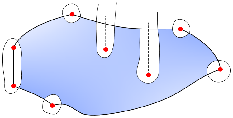
(a) A good choice of $\mathcal{U}$.

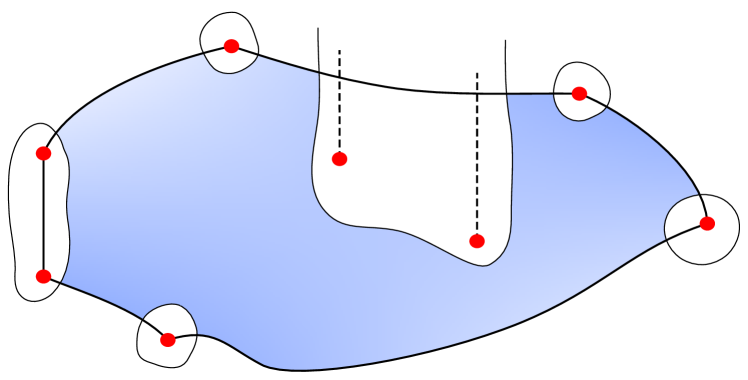
(b) A bad choice of $\mathcal{U}$, where we will miss the edge of the polygon with vertices coming from the two focus-focus values.

Figure 4: Two examples of choice of $\mathcal{U}$. In these examples $F(M)$ is compact and we take $S=\{(x,y)\in\mathbb{R}^{2}\ |\ u_{1}\leq x\leq u_{2}\}$ with $J(M)\subset[u_{1},u_{2}]$. The rank zero (elliptic-elliptic and focus-focus) critical points of $F$ are indicated by red dots, and $F(M)\cap\mathcal{U}^{c}$ is the blue filled region.

Let $c\in\mathcal{K}(S,\mathcal{U})$. By construction, $c$ is either a regular value of $F$, in which case Theorem 4.2 states that there exists an open ball $B_{c}\subset\mathcal{V}$ containing $c$ such that $(\Sigma_{\hbar}\cap B_{c},\mathcal{I},B_{c})$ is an asymptotic lattice, or a $J$-transversally elliptic value of $F$, in which case by Theorem 7.4, there exists an open ball $B_{c}\subset\mathcal{V}$ containing $c$ such that $(\Sigma_{\hbar}\cap B_{c},\mathcal{I},B_{c})$ is an asymptotic half-lattice. Since $\mathcal{K}(S,\mathcal{U})$ is compact, we can extract from the open cover $\bigcup_{c\in\mathcal{K}(S,\mathcal{U})}B_{c}\supset\mathcal{K}(S,\mathcal{U})$ a finite open cover $\bigcup_{\ell=1}^{q}B_{j}\supset\mathcal{K}(S,\mathcal{U})$ so that there exists $p\in\{0,\ldots,q\}$ such that for every $j\in\{1,\ldots,p\}$, $(\Sigma_{\hbar}\cap B_{j},\mathcal{I},B_{j})$ is an asymptotic lattice and for every $j\in\{p+1,\ldots,q\}$, $(\Sigma_{\hbar}\cap B_{j},\mathcal{I},B_{j})$ is an asymptotic half-lattice. Let $(\tilde{B}_{j})_{1\leq j\leq q}$ be a refinement of $(B_{j})_{1\leq j\leq q}$ satisfying the assumptions of Theorem 4.30 with respect to $\mathcal{L}_{\hbar}^{(i)}=\Sigma_{\hbar}\cap B_{i}$. Using this proposition, we construct two maps $\ell_{\hbar}:\Sigma_{\hbar}\cap\mathcal{K}(S,\mathcal{U})\to\mathbb{Z}^{2}$ and $\Phi:\mathcal{K}(S,\mathcal{U})\to\mathbb{R}^{2}$ and a vector $\nu_{\hbar}\in\mathbb{Z}^{2}$ such that for every $j\in\{1,\ldots,q\}$, ${\ell_{\hbar}}_{|\Sigma_{\hbar}\cap\tilde{B}_{j}}$ is a linear labelling and $\|\Phi(\lambda)-\hbar\ell_{\hbar}(\lambda)-\nu_{\hbar}\|\leq K\hbar$.

Lemma 5.9

The maps $\ell_{\hbar}$ and $\Phi$ can be chosen to be semitoric, i.e. such that for every $j\in\{1,\ldots,q\}$, ${\rm d}(\Phi_{|\tilde{B}_{j}})^{-1}(\xi_{1},\xi_{2})={\rm d}\xi_{1}$.

Proof .  Let $j\in\{1,\ldots,q\}$. We can choose a semitoric labelling $\ell_{\hbar}^{(j)}$ for $\Sigma_{\hbar}\cap B_{j}$. This comes from [27, Lemma 3.32] if $1\leq j\leq p$ and from the fact that $G_{0}^{(j)}$ in Theorem 7.4 can be chosen semitoric, see Lemma 7.1, if $p+1\leq j\leq q$. By Theorem 4.30, the choice of this labelling $\ell_{\hbar}^{(j)}$ determines $\ell_{\hbar}$. And since $G_{0}^{(j)}$ is semitoric, all the other $G_{0}^{(i)}$ must be semitoric as well. $\square$

In what follows, we will always assume that $\ell_{\hbar}$ and $\Phi$ are semitoric.

Definition 5.10

We call $\ell_{\hbar}$ a quantum cartographic map associated with $S$ and $\mathcal{U}$.

By construction of the cartographic homeomorphism (see [85, Section 5.2.2]), we have the following.

Lemma 5.11

The map $\Phi$ uniquely extends to $F(M)$ to a cartographic homeomorphism for $(M,\omega,F)$, that we still call $\Phi$. This cartographic homeomorphism corresponds to $\vec{\epsilon}=(1,\ldots,1)$, using notation from Section 2.3.

Let $d$ be the Euclidean distance on $\mathbb{R}^{2}$. Recall that the Hausdorff distance between two compact sets $K_{1},K_{2}\subset\mathbb{R}^{2}$ is defined as

$$d_{H}(K_{1},K_{2})=\inf\{\varepsilon\geq 0\ |\ K_{1}\subset K_{2}^{\varepsilon}\text{ and }K_{2}\subset K_{1}^{\varepsilon}\}$$

where $K_{j}^{\varepsilon}=\bigcup_{x\in K_{j}}\{y\in\mathbb{R}^{2}\ |\ d(x,y)\leq\varepsilon\}$.

Proposition 5.12

Let $\ell_{\hbar}$ be a quantum cartographic map associated with $S$ and $\mathcal{U}$, let $\Phi$ be the corresponding cartographic homeomorphism, let $\nu_{\hbar}$ be the corresponding vector (see Theorem 4.30) and let $\Delta_{\hbar}(\mathcal{K}(S,\mathcal{U})):=\hbar\ell_{\hbar}(\mathcal{K}(S,\mathcal{U}))$. Then the set $\nu_{\hbar}+\Delta_{\hbar}(\mathcal{K}(S,\mathcal{U}))$ converges to $\Phi(\mathcal{K}(S,\mathcal{U}))$ when $\hbar$ goes to $0$ in the sense of the Hausdorff distance. More precisely, there exists $\hbar_{1}>0$ and a constant $C>0$ such that

$$\forall\hbar\in\mathcal{I}\cap[0,\hbar_{1}]\qquad d_{H}(\nu_{\hbar}+\Delta_{\hbar}(\mathcal{K}(S,\mathcal{U})),\Phi(\mathcal{K}(S,\mathcal{U})))\leq C\hbar.$$

Proof .  Let $M$ be the maximum of $\|\operatorname{d}\!{\Phi}\|$ on $\overline{\bigcup_{i=1}^{q}B_{i}}$. Let $\xi\in\Phi(\mathcal{K}(S,\mathcal{U}))$; there exists $c\in\mathcal{K}(S,\mathcal{U})$ such that $\xi=\Phi(c)$. From [27, Lemma 3.14] and its proof (which works similarly for half-lattices), there exist a constant $C>0$, $\hbar_{1}\in\mathcal{I}$ and a family $(\lambda_{\hbar})_{\hbar\in\mathcal{I}\cap[0,\hbar_{1}]}$ such that $\forall\hbar\in\mathcal{I}\cap[0,\hbar_{1}]$, $\lambda_{\hbar}\in\mathcal{K}(S,U)$ and $\|\lambda_{\hbar}-c\|\leq C\hbar$. Let $\xi_{\hbar}=\hbar\ell_{\hbar}(\lambda_{\hbar})$; then $\xi_{\hbar}\in\Delta_{\hbar}(\mathcal{K}(S,\mathcal{U}))$ and

$$\|\nu_{\hbar}+\xi_{\hbar}-\xi\|\leq\|\nu_{\hbar}+\xi_{h}-\Phi(\lambda_{\hbar})\|+\|\Phi(\lambda_{\hbar})-\Phi(c)\|\leq(K+CM)\hbar$$

where $K$ is as in Theorem 4.30.

Conversely, let $(\xi_{\hbar})_{\hbar\in\mathcal{I}}$ be a family of elements of $\Delta_{\hbar}(\mathcal{K}(S,\mathcal{U}))$. Then there exists a family $(\lambda_{\hbar})_{\hbar\in\mathcal{I}}$ of elements of $\Sigma_{\hbar}\cap\mathcal{K}(S,\mathcal{U})$ such that for every $\hbar\in\mathcal{I}$, $\xi_{\hbar}=\hbar\ell_{\hbar}(\lambda_{\hbar})$. Then $\Phi(\lambda_{\hbar})\in\Phi(\mathcal{K}(S,\mathcal{U}))$ and

$$\|\nu_{\hbar}+\xi_{\hbar}-\Phi(\lambda_{\hbar})\|\leq K\hbar\leq(K+CM)\hbar.$$

Hence $d_{H}(\nu_{\hbar}+\Delta_{\hbar}(\mathcal{K}(S,\mathcal{U})),\Phi(\mathcal{K}(S,\mathcal{U})))\leq\tilde{C}\hbar$ with $\tilde{C}=K+CM$. $\square$

As a corollary, from the joint spectrum of a proper quantum semitoric system, we can recover the twisting index invariant of the underlying classical semitoric system.

Theorem 5.13

Let $F=(J,H)$ be a semitoric system and let $S\subset\mathbb{R}^{2}$ be a vertical strip of the form $S=\{(x,y)\in\mathbb{R}^{2}\ |\ u_{1}\leq x\leq u_{2}\}$ where $u_{1},u_{2}\notin\{x_{1},\ldots,x_{m_{f}}\}$. Given the $\hbar$-family of joint spectra $\Sigma_{\hbar}$ modulo $\mathscr{O}(\hbar^{2})$ (see Definition 3.5) of a proper quantum semitoric system $(\hat{J}_{\hbar},\hat{H}_{\hbar})$ quantizing $(J,H)$, one can recover, in a constructive way, the set $\Phi(S\cap F(M))$ and the twisting numbers associated with the polygon $\Phi(F(M))$ of the focus-focus values contained in $S$, where $\Phi$ is some cartographic homeomorphism corresponding to upwards cuts only, i.e. $\vec{\epsilon}=(1,\ldots,1)$. In particular, the knowledge of $\Sigma_{\hbar}$ modulo $\mathscr{O}(\hbar^{2})$ allows to recover the complete twisting index invariant of $F$. Moreover if $M$ is compact, we can explicitly construct this invariant from the data of these joint spectra.

Remark 5.14 When $m_{f}=0$, the system is of toric type, which means that there exists a diffeomorphism $G$ from $F(M)$ into its image such that $G\circ F$ is the momentum map of an effective $\mathbb{T}^{2}$-action on $M$. In this case, Theorem 5.13 says that we can recover its polygon invariant in compact regions. Since the polygon is the only symplectic invariant in this case, this settles the inverse spectral problem for systems of toric type. Even this seemingly simple result is new; indeed, while in the toric case the recovery of the image $F(M)$ was sufficient [19, 71], if the system is only of toric type, one needs to handle how to straighten the deformed integral affine structure, in order to recover the diffeomorphism $G$.   $\triangle$

Proof .  Recall that from Step 1 in the proof of Theorem 3.1 in [62] or from [75], we know how to recover the image of the momentum map from the joint spectrum $\Sigma_{\hbar}$, so in particular we know where the elliptic-elliptic values and potential vertical walls are located. In principle these results only apply to less general classes of semiclassical operators such as operators with uniformly bounded symbols, but as explained in [62, Section 2.4] (see also [30, Chapter 10]), we can simply microlocalize in a bounded region of phase space containing $S\cap F(M)$ to work with bounded symbols; here the properness of $(\hat{J}_{\hbar},\hat{H}_{\hbar})$ is crucial. See also Remark 5.13 for an alternative way to locate the elliptic-elliptic values and vertical walls.

Moreover, we can also detect the focus-focus values from the data of $\Sigma_{\hbar}$ up to $\mathscr{O}(\hbar^{2})$. This is done using Step 3 of the proof of Theorem 3.1 in [62], which only relies on the knowledge of a basis of the period lattice over regular values of $F$; the idea is to locate the focus-focus values using the logarithmic singularity of this basis. Here is a method to perform this detection in a more constructive way. First, by the Duistermaat-Heckman formula (Remark 5.13) we obtain the potential abscissae of the focus-focus values. Then, considering a vertical strip above each of these abscissae $x_{0}$, we may draw the graph of the vertical level spacings using Lemma 5.2. The logarithmic behavior of the coefficient $a_{2}(c)$ at the focus-focus value is enough to precisely locate that value; more precisely, from Proposition 2.5 and Equation (6) we see that, if $(x_{0},y_{0})$ is the focus-focus critical value, we have

$$a_{2}(x_{0},y)\sim C\ln\left|y-y_{0}\right|\text{ as }y\to y_{0}.$$

This is illustrated in Figure 25.

So we know the set $(V_{1}\cup\ldots\cup V_{m_{f}})\cup E\cup W$, see (21).

Let $(x_{i_{1}},y_{i_{1}}),\ldots(x_{i_{p}},y_{i_{p}})$ be the focus-focus values contained in $S$. For every $j\in\{1,\ldots,p\}$, let $r_{j}>0$ be such that $B((x_{i_{j}},y_{i_{j}}),r_{j})$ is contained in the image of an open set where Eliasson’s normal form of Theorem 2.1 is defined. Let $r=\min_{j}r_{j}>0$. Let $\varepsilon\in(0,r)$, and let $\mathcal{U}_{\varepsilon}$ be the union of $\varepsilon$-neighborhoods of every $L_{i_{j}}$ and every element of $E\cap S$ and of $W\cap S$ for some well-chosen $\varepsilon\in(0,r)$, so as to avoid problems with consecutive critical values of $F$ (see Figure 4). Let $\mathcal{K}(S,\mathcal{U}_{\varepsilon})$ be as in the beginning of this section. Of course one does not know $r$ a priori but the rest of the proof consists in investigating the limit $\varepsilon\to 0$.

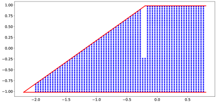
Figure 14: Determination of the privileged polygon for the spin-oscillator using Proposition 5.12; the blue dots represent the set $\Delta_{\hbar}(\mathcal{K}(S,\mathcal{U}))$ where $S=\{(x,y)\in\mathbb{R}^{2}\ |\ -0.8\leq x\leq 2\}$ for $k=25$, while the solid red lines represent a translation of the privileged semitoric polygon shown in Figure 6. Note that this translation is unavoidable because of the vector $\nu_{\hbar}$ in Proposition 5.12.

Let $\ell_{\hbar}$ be a quantum cartographic map associated with $S$ and $\mathcal{U}_{\varepsilon}$, and let $\Phi$ be the corresponding cartographic homeomorphism (Lemma 5.11 ensures that $\Phi$ does not depend on $\varepsilon$). By Proposition 5.12, we can recover the set $\Phi(\mathcal{K}(S,\mathcal{U}_{\varepsilon}))$ (note that the constants $\nu_{\hbar}$ in this proposition are not a problem since the position of the polygon $\Phi(F(M))$ in $\mathbb{R}^{2}$ does not matter). Since the set $\Phi(S\cap F(M))$ is polygonal and since we know where its vertices should be since we know the locations of elliptic-elliptic and focus-focus values and that the cuts are all upwards, and because of our choice of $\mathcal{U}_{\varepsilon}$, we can recover it from $\Phi(\mathcal{K}(S,\mathcal{U}_{\varepsilon}))$ by drawing the missing vertices and pieces of edges, see for instance Figures 14 and 26.

By construction, for every $j\in\{1,\ldots,p\}$ the restriction of $\Phi$ over some ball intersecting $(B((x_{i_{j}},y_{i_{j}}),r)\setminus B((x_{i_{j}},y_{i_{j}}),\varepsilon))\cap\{x\geq x_{i_{j}}\}$ is an action diffeomorphism, so $\Phi\circ F=(J,L_{j})$ where the action variable $L_{j}$ is independent of $\varepsilon$. So by Theorem 5.1, for every $j\in\{1,\ldots,p\}$, we can recover the invariant $\sigma_{1}((x_{i_{j}},y_{i_{j}}))$ associated with $L_{j}$, by considering $\varepsilon\to 0$ (recall that in this theorem, we first let $\hbar\to 0$ at fixed $c$ close to $(x_{i_{j}},y_{i_{j}})$ and then consider the limit $c\to(x_{i_{j}},y_{i_{j}})$). This means that we can recover the twisting numbers of the focus-focus values contained in $S$, because we compare $L_{j}$ with the privileged action $L_{\text{priv},j}$ recovered from $\Sigma_{\hbar}$ thanks to Proposition 5.8.

If $M$ is compact, then $F(M)$ is compact as well, so it suffices to take $S$ sufficiently large in order to recover the whole polygon associated with $\Phi$ and the corresponding twisting numbers, hence the twisting index invariant. $\square$

Remark 5.15 In the first part of the proof of this theorem, another (perhaps more satisfactory from an algorithmic point of view) way to locate the elliptic-elliptic values and vertical walls of the momentum map is to count the eigenvalues in suitable vertical strips. More precisely, let $\delta\in(0,\frac{1}{2})$, $c>0$ and for $x\in J(M)$, set $N_{\hbar}(x,\delta,c)=\#\Sigma_{\hbar}\cap[x-c\hbar^{\delta},x+c\hbar^{\delta}]\times\mathbb{R}$. Then

$$\frac{\hbar^{2-\delta}}{2c}N_{\hbar}(x,\delta,c)\underset{\hbar\to 0}{\longrightarrow}\rho_{J}(x)$$ (22)

where $\rho_{J}$ is the Duistermaat-Heckman function associated with $J$ [36], using notation from [93, Section 5]. We illustrate this result in Figure 24. It is standard that $\rho_{J}$ is continuous and piecewise affine and by Theorem 5.3 in the aforementioned paper, a change of slope in its graph at $(x_{0},\rho_{J}(x_{0}))$ indicates the presence of one or several elliptic-elliptic or focus-focus values in the fiber $J^{-1}(x_{0})$. The limit of the top and bottom points of this strip gives the potential positions of the elliptic-elliptic values, as in Remark 4.14. Of course the Duistermaat-Heckman function cannot tell us whether the elliptic point lies at the bottom or at the top of the strip (or both), but in view of the rest of the proof, it is not an issue. Indeed, we may add extra isolated points (corresponding to transversally elliptic critical values) to the set $E$. It does not prevent the reconstruction of the polygon from the joint spectrum, thanks to the data of the surrounding edges. The corners of the polygon will finally tell where the true elliptic-elliptic singular values were located. Furthermore, we know that the potential vertical walls can only be located at the global minimum or maximum of $J$, and their existence would be equivalent to the fact that $\rho_{J}$ is nonzero at these points.

Equation (22) is nothing but Weyl’s law for $\hat{J}_{\hbar}$ in an interval of size $\hbar^{\delta}$. Its proof is similar to the usual case of a fixed interval, see for instance [101, Theorem 14.11]. However one needs to use the fact that if $\chi$ is a compactly supported smooth function and $P_{\hbar}$ is a semiclassical operator in $S(m)$, $\chi(\hbar^{-\delta}P_{\hbar})$ is a semiclassical operator in $S_{\delta}(m)$, and asymptotic estimates for the trace of a semiclassical operator with symbol in a class $S_{\delta}(m)$, see for instance [101, Section 4.4] for the definition of these classes. These results are known for $\hbar$-pseudodifferential operators: for instance, the former can be derived by adapting the arguments in [87, Section 8], and the latter can be obtained from the usual estimate for the trace of an operator in $S(m)$ and a rescaling of the semiclassical parameter. While they have not yet been proved for Berezin-Toeplitz operators, there is no doubt that they also hold in this context. Another important point in the derivation of (22) is that $\rho_{J}$ is Lipschitz.   $\triangle$

6 Recovering the Taylor series invariant from the joint spectrum

In this section, we continue to work in a neighborhood $B$ of a simple focus-focus critical value $0\in\mathbb{R}^{2}$, for the completely integrable momentum map $F=(J,H)$. We carry on the analysis of the spectrum of a proper quantum integrable system $(\hat{J}_{\hbar},\hat{H}_{\hbar})$ associated with the momentum map $F$ started in Section 4 to recover the Taylor series invariant and the height invariant, both defined in Section 2.5. The study of the height invariant led us to investigate the behavior of the number of points in an asymptotic lattice.

Prior to this work, it was unknown whether the joint spectrum of $(\hat{J}_{\hbar},\hat{H}_{\hbar})$ near $0$ fully determines $F$, up to symplectic equivalence. An important first step was proven in [77]: the joint spectrum, restricted to the small neighborhood $B$, determines the Taylor series invariant. This was an uniqueness statement, whose precise meaning was that whenever the joint spectra of two such quantum integrable systems coincide up to $\mathscr{O}(\hbar^{2})$, then their Taylor series invariants coincide. However, no method of construction of the invariant from the joint spectrum was given. In this section, we are interested only in the semitoric case, but the result we show is quite stronger, namely that the Taylor series invariant can be constructed from the joint spectrum of a single semitoric system near a focus-focus critical value. This Taylor series invariant determines $F$ near the critical fiber $F^{-1}(0)$ up to left-composition by a local diffeomorphism. In fact, we obtain a better result since we also recover the full Taylor series of the Eliasson diffeomorphism, which completely characterizes $F$ up to a flat term. Actually, our constructions also allow the recovery of the Taylor series invariant and the infinite jet of the Eliasson diffeomorphism for focus-focus singularities in systems that are not necessarily semitoric.

To our knowledge, constructive statements in inverse spectral theory are not so common; however, a constructive way to compute the linear terms of the Taylor series invariant was proposed in [76], under the assumption that the singular Bohr-Sommerfeld conditions hold; here we want to avoid this assumption in the context of Berezin-Toeplitz quantization, since the corresponding Bohr-Sommerfeld conditions have not been proven yet.

6.1 The height invariant

As explained in Section 2.5, the height invariant can be considered as the constant term $S_{0,0}$ of the Taylor series invariant. It has been computed explicitly for some specific classical systems in [76, 60, 2, 1]. In [62], it was proven that if two quantum semitoric systems have the same semiclassical joint spectrum, then they must share the same height invariant. In this section, we take another route and obtain a direct formula for computing this invariant from a single semiclassical joint spectrum. Since the height invariant has an intrinsic definition in terms of a symplectic volume, a natural way to recover it from the joint spectrum is to make use of a suitable Weyl formula. Hence, this method is quite different from the way the higher order invariants will be handled in the following sections.

Proposition 6.1

The height invariant $S_{0,0}$ associated with the focus-focus critical value $c_{0}=0$ can be explicitly recovered from the joint spectrum modulo $\mathscr{O}(\hbar^{2})$ in a vertical strip below $c_{0}$ by the following formula. Let $\delta\in(0,\frac{1}{2})$, $c>0$ and $y\geq 0$, and define $N_{\hbar}(\delta,c,y)=\#\Sigma_{\hbar}\cap[-c\hbar^{\delta},c\hbar^{\delta}]\times(-\infty,-y]$. Then

$$S_{0,0}=\lim_{y\to 0}\lim_{\hbar\to 0}\frac{\hbar^{2-\delta}}{2c}N_{\hbar}(\delta,c,y).$$ (23)

Furthermore,

$$S_{0,0}=\lim_{\hbar\to 0}\frac{\hbar^{2-\delta}}{2c}N_{\hbar}(\delta,c,0).$$ (24)

In order to prove this proposition we need to discuss general results concerning counting functions in asymptotic lattices or half-lattices.

Lemma 6.2

Let $(\mathcal{L}_{\hbar},\mathcal{I},B)$ be an asymptotic lattice or half-lattice, and let $\Gamma\subset B$ be a compact, smooth curve immersed in $B$. Let $\Gamma_{\hbar}$ be a thickening of $\Gamma$ of width $\mathscr{O}(\hbar)$. Let $N_{\hbar}(\Gamma_{\hbar})$ be the cardinal of $\mathcal{L}_{\hbar}\cap\Gamma_{\hbar}$. Then

$$N_{\hbar}(\Gamma_{\hbar})=\mathscr{O}\Big{(}\frac{1}{\hbar}\Big{)}.$$

Proof .  We may cover $\Gamma_{\hbar}$ by a number $n_{\hbar}$ of balls of radius $C\hbar$, where $C>0$ is large enough and the center of each ball belongs to $\Gamma$, in such a way that $n_{\hbar}\sim\frac{L}{C\hbar}$ for some $L>0$ ($L$ will be proportional to the length of $\Gamma$). By the properties of asymptotic (half-)lattices, the number of points in each ball is bounded by a uniform constant independent of $\hbar$. $\square$

Lemma 6.3

Let $(\mathcal{L}_{\hbar},\mathcal{I},B)$ be an asymptotic lattice or half-lattice, and let $\tilde{B}\Subset B$ be a domain with piecewise smooth boundary $\Gamma$. Let $N_{\hbar}(\tilde{B})$ be the cardinal of $\mathcal{L}_{\hbar}\cap\tilde{B}$. Then

$$N_{\hbar}(\tilde{B})=\frac{1}{\hbar^{2}}\emph{area}(G_{0}^{-1}(\tilde{B}\cap\underline{\mathcal{L}_{\hbar}}))+\mathscr{O}(\frac{1}{\hbar}),$$

where $G_{0}$ is the leading term of an asymptotic chart for $\mathcal{L}_{\hbar}$, and the set $\underline{\mathcal{L}_{\hbar}}$ was defined in Lemma 4.21 (it does not depend on $\hbar$).

Proof .  Let $G_{\hbar}$ be an asymptotic chart for $B$. In the case of an asymptotic lattice (the case of an asymptotic half-lattice is similar, upon replacing $\tilde{B}$ by $\tilde{B}\cap\underline{\mathcal{L}_{\hbar}}$), we have

$$N_{\hbar}(\tilde{B})=\#\{\lambda_{\hbar}\in\tilde{B}\}\simeq\#\{\zeta\in\mathbb{Z}^{2}\ |\ G_{\hbar}(\hbar\zeta)\in\tilde{B}\},$$

and the approximation $\simeq$ is in general non exact because $G_{\hbar}(\hbar\zeta)$ approaches $\lambda_{\hbar}$ only up to $\mathscr{O}(\hbar^{\infty})$, which is enough for points close to the boundary $\Gamma$ to escape $\tilde{B}$ under this perturbation. However, for any $B^{\prime}\subset B$, let us introduce $M_{\hbar}(B^{\prime}):=\#\{\zeta\in\mathbb{Z}^{2}\ |\ G_{\hbar}(\hbar\zeta)\in B^{\prime}\}$; then the following inequalities are exact, for $\hbar$ small enough:

$$M_{\hbar}(\tilde{B}^{-}_{\hbar})\leq N_{\hbar}(\tilde{B})\leq M_{\hbar}(\tilde{B}^{+}_{\hbar}),$$

where $\tilde{B}^{-}_{\hbar}$ is an $\hbar$-shrinking of $\tilde{B}$, and $\tilde{B}^{+}_{\hbar}$ an $\hbar$-enlarging, such that $\tilde{B}^{-}_{\hbar}\subset\tilde{B}\subset\tilde{B}^{+}_{\hbar}$ and $\Gamma_{\hbar}:=\tilde{B}^{+}_{\hbar}\setminus\tilde{B}^{-}_{\hbar}$ is an $\hbar$-thickening of $\Gamma$, as in Lemma 6.2. Applying that lemma yields

$$N_{\hbar}(\tilde{B})=M_{\hbar}(\tilde{B}^{\pm}_{\hbar})+\mathscr{O}(\frac{1}{\hbar})=M_{\hbar}(\tilde{B})+\mathscr{O}(\frac{1}{\hbar}).$$

Similarly, since $G_{\hbar}=G_{0}+\mathscr{O}(\hbar)$ uniformly on $\tilde{B}$, we may replace $G_{\hbar}$ by $G_{0}$ in the above estimates:

$$N_{\hbar}(\tilde{B})=M_{0,\hbar}(\tilde{B})+\mathscr{O}(\frac{1}{\hbar}),$$ (25)

with $M_{0,\hbar}(\tilde{B}):=\#\{\zeta\in\mathbb{Z}^{2}\ |\ G_{0}(\hbar\zeta)\in\tilde{B}\}$. Finally, we notice that $\hbar^{2}M_{0,\hbar}(\tilde{B})$ is a Riemann approximation of the integral $\int_{G_{0}^{-1}(\tilde{B})}\operatorname{d}\!{\zeta}=\textup{area}(G_{0}^{-1}(\tilde{B}))$:

$$\hbar^{2}M_{0,\hbar}(\tilde{B})=\textup{area}(G_{0}^{-1}(\tilde{B}))+\mathscr{O}(\hbar).$$

Together with (25), this proves the lemma. $\square$

Proof of Proposition 6.1.   It follows from the Bohr-Sommerfeld rules (regular, see Theorem 4.2, and elliptic, see Theorem 7.4) that, away from focus-focus critical values, the joint spectrum $\Sigma_{\hbar}$ is locally an asymptotic lattice or half-lattice. Hence, for any rectangle $R$ containing only regular values or transversally elliptic critical values of $F$, the number of joint eigenvalues inside $R$ is

$$N_{\hbar}(R)=\frac{1}{\hbar^{2}}\int_{R\cap\underline{\Sigma_{\hbar}}}\left|\operatorname{d}\!{\Phi}\right|\operatorname{d}\!{c}+\mathscr{O}(\frac{1}{\hbar}),$$ (26)

where the map $\Phi$ was obtained in Theorem 4.30, and $\left|\operatorname{d}\!{\Phi}\right|$ denotes its Jacobian. Indeed, $R$ can be covered by asymptotic lattices or half-lattices, and in each one we may find an asymptotic chart $G_{\hbar}$, such that $\operatorname{d}\!{\Phi}=\operatorname{d}\!{G}_{0}^{-1}$; hence we may apply Lemma 6.3 and we see that the integrals $\int_{G_{0}^{-1}(\tilde{B})}\operatorname{d}\!{\zeta}=\int_{\tilde{B}}\left|\operatorname{d}\!{G}_{0}^{-1}\right|\operatorname{d}\!{c}$ nicely patch together to give (26).

Now, we know from the Bohr-Sommerfeld analysis that $G_{0}^{-1}$ is actually an action diffeomorphism. Therefore, the change of coordinates $\zeta=G_{0}^{-1}(c)$ gives the density $\left|\operatorname{d}\!{G}_{0}^{-1}\right|\operatorname{d}\!{c}=\operatorname{d}\!{\zeta}=\frac{1}{(2\pi)^{2}}\operatorname{d}\!{\zeta}\int\operatorname{d}\!{\theta}$, where $(\zeta,\theta)$ are action-angle coordinates. Since $F=G_{0}\circ\zeta$, we have $\int_{\tilde{B}}\left|\operatorname{d}\!{G}_{0}^{-1}\right|\operatorname{d}\!{c}=\frac{1}{(2\pi)^{2}}\textup{Vol}(F^{-1}(\tilde{B}))$, where Vol is the usual symplectic volume in $M$. This gives

$$\int_{R\cap\underline{\Sigma_{\hbar}}}\left|\operatorname{d}\!{\Phi}\right|\operatorname{d}\!{c}=\frac{1}{(2\pi)^{2}}\textup{Vol}(F^{-1}(R\cap\underline{\Sigma_{\hbar}}))=\frac{1}{(2\pi)^{2}}\textup{Vol}(F^{-1}(R)),$$

since $\underline{\Sigma_{\hbar}}\subset F(M)$. Thus, Equation (26) gives the following “joint Weyl formula”:

$$N_{\hbar}(R)=\frac{1}{(2\pi\hbar)^{2}}\textup{Vol}(F^{-1}(R))+\mathscr{O}(\hbar^{-1}),$$ (27)

Notice that the formula is uniform in $R$, as long as $R$ stays in a fixed compact region.

By a simple scaling argument, we may assume without loss of generality that the constant $c$ in the proposition is $c=1$. Let $\delta\in(0,\frac{1}{2})$, and let $S_{\delta}\subset\mathbb{R}^{2}$ be a vertical strip of width $2\hbar^{\delta}$ around the focus-focus value $c_{0}=0$, i.e. $S_{\delta}=[-\hbar^{\delta},\hbar^{\delta}]\times\mathbb{R}$. Let $y\geq 0$, and split $S_{\delta}$ vertically in three parts, $S_{\delta}^{-}(y)$, $S_{\delta}^{0}(y)$, and $S_{\delta}^{+}(y)$, namely:

$$S_{\delta}^{-}(y)=[-\hbar^{\delta},\hbar^{\delta}]\times(-\infty,-y],\quad S_{\delta}^{0}(y)=[-\hbar^{\delta},\hbar^{\delta}]\times(-y,y),\quad S_{\delta}^{+}(y)=[-\hbar^{\delta},\hbar^{\delta}]\times[y,+\infty).$$

The set $S_{\delta}^{0}(y)$ contains the focus-focus value, and the joint spectrum near this value is neither an asymptotic lattice nor an asymptotic half-lattice. Let $y>0$, so that $N_{\hbar}(\delta,1,y)=N_{\hbar}(S_{\delta}^{-}(y))$. From (27) we have

$$N_{\hbar}(S_{\delta}^{-}(y))=\frac{1}{(2\pi\hbar)^{2}}\textup{Vol}(F^{-1}(S_{\delta}^{-}(y)))+\mathscr{O}(\hbar^{-1}).$$ (28)

Near any point $m\in M$ where $\operatorname{d}\!{J}(m)\neq 0$, we can write the symplectic measure as $\left|\omega^{2}\right|/2=\left|\omega_{x}\right|\wedge\operatorname{d}\!{J}\wedge\operatorname{d}\!{\theta}$, where $\omega_{x}$ is the natural symplectic form on the local reduced manifold $J^{-1}(x)/\mathcal{X}_{J}$, $x=J(m)$, and $\theta$ is the angle expressing the time of the Hamiltonian flow of $J$. Hence

$$\textup{Vol}(F^{-1}(S_{\delta}^{-}(y))) =\int_{-\hbar^{\delta}}^{\hbar^{\delta}}\operatorname{d}\!{x}\int_{F^{-1}(\{x\}\times(-C,-y])}\left|\omega_{x}\right|\wedge\operatorname{d}\!{\theta}$$

$$=\int_{-\hbar^{\delta}}^{\hbar^{\delta}}\operatorname{d}\!{x}\int_{F^{-1}(\{0\}\times(-C,-y])}\left|\omega_{0}\right|\wedge\operatorname{d}\!{\theta}+\mathscr{O}(x)$$

$$=2\hbar^{\delta}\int_{F^{-1}(\{0\}\times(-C,-y])}\left|\omega_{0}\right|\wedge\operatorname{d}\!{\theta}+\mathscr{O}(\hbar^{2\delta}).$$

Notice that $\int_{F^{-1}(\{0\}\times(-C,-y])}\left|\omega_{0}\right|\wedge\operatorname{d}\!{\theta}=2\pi\textup{Vol}_{0}^{-}(y)$, where $\textup{Vol}_{0}^{-}(y)$ is the volume of the sublevel set $H\leq y$ within the reduced symplectic orbifold $M_{0}:=J^{-1}(0)/\mathcal{X}_{J}$. This gives

$$\frac{\textup{Vol}(F^{-1}(S_{\delta}^{-}(y)))}{2\hbar^{\delta}}=2\pi\textup{Vol}_{0}^{-}(y)+\mathscr{O}(\hbar^{\delta}).$$ (29)

We know from the local analysis of focus-focus singularities (see for instance [93]) that

$$\textup{Vol}_{0}^{\pm}(y)=\textup{Vol}_{0}^{\pm}(0)+\mathscr{O}(y\log y).$$ (30)

Together with (28), since the height invariant is precisely $S_{0,0}=\frac{1}{2\pi}\textup{Vol}_{0}^{-}(0)$, this gives (23).

To prove (24), observe that by simple inclusions, we have

$$N_{\hbar}(S_{\delta}^{-}(y))\leq N_{\hbar}(S_{\delta}^{-}(0))\leq N_{\hbar}(S_{\delta})-N_{\hbar}(S_{\delta}^{+}(y)).$$ (31)

Since $J$ is proper, the vertical extent of joint eigenvalues in the strip $S_{\delta}$ is actually bounded; hence in the above formula one may replace $S_{\delta}^{-}(y)$ by a suitable rectangle $[-\hbar^{\delta},\hbar^{\delta}]\times(-C,-y]$, and similarly for $S_{\delta}^{+}(y)$.

Of course, an analogous formula holds for $S_{\delta}^{+}(y)$. Therefore, multiplying Equation (31) by $\hbar^{2-\delta}/2$ and taking the limit inferior when $\hbar\to 0$ yields, in view of (22),

$$(2\pi)^{-1}\textup{Vol}_{0}^{-}(y)\leq\liminf_{\hbar\to 0}\hbar^{2-\delta}N_{\hbar}(S_{\delta}^{-}(0))/2\leq(2\pi)^{-1}(\textup{Vol}_{0}-\textup{Vol}_{0}^{+}(y)),$$

where $\textup{Vol}_{0}$ is the complete volume of $M_{0}$.

Using Equation (30) again, and since $\textup{Vol}_{0}=\textup{Vol}_{0}^{-}(0)+\textup{Vol}_{0}^{+}(0)$, we get, when $y\to 0$,

$$0\leq\liminf_{\hbar\to 0}\frac{\hbar^{2-\delta}}{2}N_{\hbar}(S_{\delta}^{-}(0))-\frac{1}{2\pi}\textup{Vol}_{0}^{-}(0)\leq 0.$$

The same holds for the limit superior, which proves the second statement of the proposition. $\square$

Remark 6.4 The “joint Weyl formula” (27) can be found in [15] in the pseudodifferential case when $R$ consists only of regular values. Including elliptic critical values (and Berezin-Toeplitz quantization), albeit not surprising, seems to be new.   $\triangle$

Remark 6.5 It would be interesting to obtain the remainder term, or at least estimate the convergence speed in this joint Weyl formula. However, it is not accessible directly with the results of the present article. For instance, in view of the pseudodifferential analysis carried out in [91], it is expected that the remainder $\mathscr{O}(\hbar^{\delta})$ in (29) cannot be uniform as $y\to 0$, because of the logarithmic accumulation of joint eigenvalues at the origin, as $\hbar\to 0$.   $\triangle$

6.2 Linear terms

The linear and higher order terms in the Taylor series invariant are obtained from the joint spectrum in slightly different ways.

From Theorem 5.1 and Proposition 5.8, we see that we can recover the first linear term $[S_{1,0}]$ of the Taylor series invariant from the joint spectrum; indeed, recall that $\sigma_{1}^{\text{p}}(0)=S_{1,0}$. Note that recovering $[S_{1,0}]$ was already achieved in [60] but again under the assumption that the singular Bohr-Sommerfeld rules hold, which is only a conjecture for the case of Berezin-Toeplitz operators, as explained above.

In order to recover the term $S_{0,1}$, we proceed similarly to the way we recovered $S_{1,0}$; as in Lemma 2.7 above, let $B_{1}\ni x\mapsto(x,\varphi(x))$ be a parametrization of the radial curve $\gamma_{r}$ near the origin. Recall that a choice of local action variable $L$ yields the two functions $\tau_{1},\tau_{2}$ defined in Equation (3).

Lemma 6.6

The function $x\mapsto\tau_{2}(x,\varphi(x))+\frac{\ln x}{2\pi}$ defined for $x\in\mathbb{R}^{*}_{+}\cap B_{1}$ is smooth at $x=0$, and its value at zero is equal to $\sigma_{2}(0)=S_{0,1}$.

Proof .  This is similar to Lemma 2.7. We know from Proposition 2.5 that the function

$$\eta:c\mapsto\tau_{2}(c)+\frac{1}{2\pi}\Re(\log\ z)$$

is smooth at $c=(0,0)$, where $z=z_{1}+iz_{2}$ with $(z_{1},z_{2})=(c_{1},f_{r}(c_{1},c_{2}))$, and that its value at the origin is $S_{0,1}$. Hence, with $w_{\varphi}(x):=x+if_{r}(x,\varphi(x))$, we have

$$x\mapsto\tau_{2}(x,\varphi(x))+\frac{1}{2\pi}\ln\left|w_{\varphi}(x)\right|=\tau_{2}(x,\varphi(x))+\frac{\ln x}{2\pi}$$

is smooth at $x=0$ and its value at this point is $S_{0,1}$. $\square$

Lemma 6.7

In order to compute the above limit to obtain $\sigma_{2}(0)$, one can replace $\gamma_{r}$ with a curve $\gamma$ which is tangent to $\gamma_{r}$ at the origin.

Proof .  We argue as in the proof of Lemma 5.4. Let $\gamma$ be any curve that is tangent to $\gamma_{r}$ at the origin; it is locally the graph of a smooth function $\psi$. Keeping the notation introduced in the proof of the previous lemma, we have that

$$x\mapsto\eta(x,\psi(x))=\tau_{2}(x,\psi(x))+\frac{1}{2\pi}\Re(\log(w_{\psi}(x)))$$

is smooth at $x=0$, and that $\eta(x,\psi(x))-\eta(x,\varphi(x))\underset{x\to 0}{\longrightarrow}0$ since $\psi(0)=0=\varphi(0)$. Hence

$$\tau_{2}(x,\psi(x))-\tau_{2}(x,\varphi(x))+\frac{1}{2\pi}\Re(\log(w_{\varphi}(x)))-\frac{1}{2\pi}\Re(\log(w_{\psi}(x)))\underset{x\to 0}{\longrightarrow}0,$$

so in view of the proof of the previous lemma, it suffices to show that

$$\Re(\log(w_{\varphi}(x)))-\Re(\log(w_{\psi}(x)))=\ln\left|w_{\varphi}(x)\right|-\ln x\underset{x\to 0}{\longrightarrow}0.$$

We can rewrite this quantity as

$$\ln\left|1+i\frac{f_{r}(x,\varphi(x))}{x}\right|=\frac{1}{2}\ln\left(1+\frac{f_{r}(x,\varphi(x))^{2}}{x^{2}}\right).$$

But we showed in the proof of Lemma 5.4 that

$$\frac{f_{r}(x,\varphi(x))}{x}\underset{x\to 0}{\longrightarrow}0,$$

so the above quantity indeed goes to zero when $x\to 0$. $\square$

Proposition 6.8

From the $\hbar$-family of joint spectra $\Sigma_{\hbar}$ of a proper quantum semitoric system in a neighborhood of a focus-focus critical value $c_{0}=0$, one can recover, in a constructive way, the symplectic invariant $S_{0,1}=\sigma_{2}(0)$.

Proof .

Step 1.

As before, and in view of the previous lemma, we consider the curve given by $x\mapsto(x,s(0)x)$. Recall that from the joint spectrum, one can recover $s(0)$ as well as $\partial_{y}f_{r}(0)$, see Lemma 5.5 and Formula (19).

Step 2.

We use once again the above lemmas and Equation (6) to write

$$\frac{a_{2}(x,s(0)x)}{\partial_{y}f_{r}(x,s(0)x)}+\frac{\ln x}{2\pi}\underset{x\to 0^{+}}{\longrightarrow}\sigma_{2}(0).$$

Since $\partial_{y}f_{r}(x,s(0)x)=\partial_{y}f_{r}(0)+\mathscr{O}(x)$, we obtain that

$$\frac{a_{2}(x,s(0)x)}{\partial_{y}f_{r}(x,s(0)x)}+\frac{\ln x}{2\pi}=\frac{a_{2}(x,s(0)x)}{\partial_{y}f_{r}(0)}(1+\mathscr{O}(x))+\frac{\ln x}{2\pi}=\frac{a_{2}(x,s(0)x)}{\partial_{y}f_{r}(0)}+\frac{\ln x}{2\pi}+\mathscr{O}(x\ln x),$$

where the last equality comes from the fact that $a_{2}(x,s(0)x)\sim-\frac{\partial_{y}f_{r}(0)}{2\pi}\ln x$ when $x\to 0^{+}$. Hence

$$\frac{a_{2}(x,s(0)x)}{\partial_{y}f_{r}(0)}+\frac{\ln x}{2\pi}\underset{x\to 0}{\longrightarrow}\sigma_{2}(0)$$

and all the quantities on the left-hand side have been recovered from the spectrum by considering good labellings in earlier parts of the paper ($a_{2}$ in Lemma 5.2, $\partial_{y}f_{r}(0)$ and $s(0)$ in Lemma 5.5). $\square$

Remark 6.9 This implies, together with Lemma 5.2, that

$$S_{0,1}=\lim_{x\to 0^{+}}\lim_{\hbar\to 0}\left(\frac{\hbar}{\partial_{y}f_{r}(0)(E_{j,\ell+1}-E_{j,\ell})}+\frac{\ln x}{2\pi}\right)$$ (32)

where $(\lambda_{j,\ell})_{j,\ell}=(J_{j,l},E_{j,\ell})_{j,\ell}$ is a good labelling and, in the above equation, $j,\ell$ are $\hbar$-dependent integers such that the joint eigenvalues $\lambda_{j,\ell}$, $\lambda_{j+1,\ell}$ and $\lambda_{j,\ell+1}$ are well-defined in an $\mathscr{O}(\hbar)$-neighborhood of $(x,s(0)x)$.   $\triangle$

6.3 Higher order terms

We show in this section how to recover all terms of the Taylor series invariant from the joint spectrum. The difficulty is that the Taylor series $S$ is defined in terms of the normal form coordinates, i.e. in terms of the function $f_{r}$ (or, more precisely, of its Taylor series at the origin $[f_{r}]$), but this function is also unknown a priori. Hence we need to find a scheme to recover, from the joint eigenvalues, both Taylor series $S$ and $[f_{r}]$ simultaneously.

In order to organize the proof, we will treat the coefficients $S_{\alpha}$ and all derivatives of $f_{r}$ at the origin as formal indeterminates, and use the following notation. Let $\mu$ be an additional formal parameter. Let $\mathcal{F}_{\leq n_{1},\leq n_{2}}$ be the polynomial algebra in the variables $\partial^{\beta}f_{r}(0)$ with $\left|\beta\right|\leq n_{1}$, in the variables $S_{\alpha}$ with $\left|\alpha\right|\leq n_{2}$, and in $\mu$. We will also use the subscript “$n_{j}$” instead of “$\leq n_{j}$” to indicate that only derivatives of order exactly $n_{j}$ are concerned.

Let $a_{1},a_{2}$ be the functions defined in Equation (5) after a choice of action variable $L$.

Proposition 6.10

Let $\mu>0$; the function

$$g_{\mu}(x):=a_{1}(x,\mu x)+\mu a_{2}(x,\mu x)\qquad\forall x>0$$

admits an asymptotic expansion of the form

$$g_{\mu}(x)\sim\sum_{n\geq 0}x^{n}(c_{n}(\mu)+d_{n}(\mu)\ln x)\qquad\text{ as }x\to 0^{+}.$$ (33)

Moreover, for $n\geq 0$, $d_{n}(\mu)\in\mathcal{F}_{n+1,0}$, namely:

$$d_{n}(\mu)=-\frac{1}{2\pi n!}\sum_{\ell=0}^{n+1}\binom{n+1}{\ell}\mu^{n+1-\ell}\partial_{x}^{\ell}\partial_{y}^{n+1-\ell}f_{r}(0)$$ (34)

and $c_{n}(\mu)\in\mathcal{F}_{\leq n+1,\leq n}\oplus\mathcal{F}_{1,n+1}$, namely:

$$c_{n}(\mu)=\tilde{c}_{n}(\mu)+\sum_{\ell=0}^{n+1}\mu^{n-\ell}\Big{(}\mu(n+1)\partial_{y}f_{r}(0)+(n-\ell+1)\partial_{x}f_{r}(0)\Big{)}S_{\ell,n+1-\ell}.$$ (35)

Here we slightly abuse notation and use the convention $(n-\ell+1)\mu^{n-\ell}=0$ if $\ell=n+1$ for the sake of simplicity.

Proof .  Let $\mu\in\mathbb{R}$. If $F:\mathbb{R}^{2}\to\mathbb{R}$ is a smooth function, one readily checks, for instance by first Taylor expanding in $\mu$, or by induction, or by using Faà di Bruno’s formula, that the coefficient in front of $x^{n}$ in the Taylor series expansion of $x\mapsto F(x,\mu x)$ at zero is

$$\frac{1}{n!}\sum_{\ell=0}^{n}\binom{n}{\ell}\mu^{n-\ell}\partial^{\ell}_{x}\partial^{n-\ell}_{y}F(0).$$

By Equation (6), $a_{2}(x,\mu x)=\tau_{2}(x,\mu x)\partial_{y}f_{r}(x,\mu x)$, which gives thanks to Proposition 2.5

$$a_{2}(x,\mu x)=\left(\sigma_{2}(x,\mu x)-\frac{1}{2\pi}\ln x-\frac{1}{4\pi}\ln\left(1+\left(\frac{f_{r}(x,\mu x)}{x}\right)^{2}\right)\right)\partial_{y}f_{r}(x,\mu x).$$

Since $f_{r}(0)=0$, the function $x\mapsto\frac{f_{r}(x,\mu x)}{x}$ is smooth at $x=0$; since moreover $\sigma_{2}$ and $\partial_{y}f_{r}$ are smooth, this implies that $x\mapsto a_{2}(x,\mu x)$ has an asymptotic expansion of the form (33). Moreover, the coefficient of $x^{n}\ln x$ in this expansion is equal to $-\frac{1}{2\pi}$ times the coefficient of $x^{n}$ in the Taylor series expansion of $x\mapsto\partial_{y}f_{r}(x,\mu x)$, namely

$$-\frac{1}{2\pi n!}\sum_{\ell=0}^{n}\binom{n}{\ell}\mu^{n-\ell}\partial^{\ell}_{x}\partial^{n-\ell+1}_{y}f_{r}(0).$$

The coefficient of $x^{n}$ in this expansion is the sum of the coefficients of $x^{n}$ in the respective Taylor series expansions of $\sigma_{2}(x,\mu x)\partial_{y}f_{r}(x,\mu x)$ and $-\frac{1}{4\pi}\ln\left(1+\left(\frac{f_{r}(x,\mu x)}{x}\right)^{2}\right)\partial_{y}f_{r}(x,\mu x)$. The latter clearly lies in $\mathcal{F}_{\leq n+1,0}$. The former is obtained as the sum

$$\sum_{k=0}^{n}[\sigma_{2}(\cdot,\mu\cdot)]_{k}[\partial_{y}f_{r}(\cdot,\mu\cdot)]_{n-k}.$$

Here we denote by $[F]_{k}$ the coefficient of $x^{k}$ in the Taylor series expansion at $0$ of a function $F\in C^{\infty}(\mathbb{R},\mathbb{R})$. But whenever $k\leq n-1$, $[\sigma_{2}(\cdot,\mu\cdot)]_{k}[\partial_{y}f_{r}(\cdot,\mu\cdot)]_{n-k}$ belongs to the algebra generated by the $\partial^{\alpha}f_{r}(0)$ with $|\alpha|\leq n+1$ and the $\partial^{\beta}\sigma_{2}(0)$ with $|\beta|\leq n-1$; the latter correspond to the $S_{\gamma}$ with $|\gamma|\leq n$ since, by definition of the Taylor series invariant,

$$\partial^{\beta}\sigma_{2}(0)=\beta_{1}!(\beta_{2}+1)!S_{\beta+(0,1)}.$$

Therefore, for our purpose we need to understand only the term corresponding to $k=n$, i.e. $[\sigma_{2}(\cdot,\mu\cdot)]_{n}[\partial_{y}f_{r}(\cdot,\mu\cdot)]_{0}$, which equals

$$\frac{\partial_{y}f_{r}(0)}{n!}\sum_{\ell=0}^{n}\mu^{n-\ell}\binom{n}{\ell}\partial_{x}^{\ell}\partial_{y}^{n-\ell}\sigma_{2}(0)=\partial_{y}f_{r}(0)\sum_{\ell=0}^{n}\mu^{n-\ell}(n-\ell+1)S_{\ell,n-\ell+1}.$$

Similarly, Equation (6) gives

$$a_{1}(x,\mu x)=\tau_{1}(x,\mu x)+\tau_{2}(x,\mu x)\partial_{x}f_{r}(x,\mu x)$$

and Proposition 2.5 yields

$$\begin{split}a_{1}(x,\mu x)&=\sigma_{1}(x,\mu x)-\frac{1}{2\pi}\arctan\left(\frac{f_{r}(x,\mu x)}{x}\right)\\ &+\left(\sigma_{2}(x,\mu x)-\frac{1}{2\pi}\ln x-\frac{1}{4\pi}\ln\left(1+\left(\frac{f_{r}(x,\mu x)}{x}\right)^{2}\right)\right)\partial_{x}f_{r}(x,\mu x).\end{split}$$

Similar arguments as above show that $x\mapsto a_{1}(x,\mu x)$ has an asymptotic expansion of the form (33), and the coefficient of $x^{n}\ln x$ in this expansion is

$$-\frac{1}{2\pi n!}\sum_{\ell=0}^{n}\binom{n}{\ell}\mu^{n-\ell}\partial^{\ell+1}_{x}\partial^{n-\ell}_{y}f_{r}(0).$$

The coefficient of $x^{n}$ in this expansion is the sum of the coefficients of $x^{n}$ in the respective Taylor series expansions of $\sigma_{1}(x,\mu x)$, $\sigma_{2}(x,\mu x)\partial_{x}f_{r}(x,\mu x)$, $-\frac{1}{2\pi}\arctan\left(\frac{f_{r}(x,\mu x)}{x}\right)$, and $-\frac{1}{4\pi}\ln\left(1+\left(\frac{f_{r}(x,\mu x)}{x}\right)^{2}\right)\partial_{x}f_{r}(x,\mu x)$. The last two belong to $\mathcal{F}_{\leq n+1,0}$. Moreover,

$$[\sigma_{1}(\cdot,\mu\cdot)]_{n}=\frac{1}{n!}\sum_{\ell=0}^{n}\mu^{n-\ell}\binom{n}{\ell}\partial_{x}^{\ell}\partial_{y}^{n-\ell}\sigma_{1}(0)=\sum_{\ell=0}^{n}\mu^{n-\ell}(\ell+1)S_{\ell+1,n-\ell},$$

and we can decompose

$$[\sigma_{2}(\cdot,\mu\cdot)\partial_{x}f_{r}(\cdot,\mu\cdot)]_{n}=\sum_{k=0}^{n-1}[\sigma_{2}(\cdot,\mu\cdot)]_{k}[\partial_{x}f_{r}(\cdot,\mu\cdot)]_{n-k}+[\sigma_{2}(\cdot,\mu\cdot)]_{n}[\partial_{x}f_{r}(\cdot,\mu\cdot)]_{0}$$

where the first term on the right-hand side lies in $\mathcal{F}_{n+1,n}$, and the second term reads

$$\frac{\partial_{x}f_{r}(0)}{n!}\sum_{\ell=0}^{n}\mu^{n-\ell}\binom{n}{\ell}\partial_{x}^{\ell}\partial_{y}^{n-\ell}\sigma_{2}(0)=\partial_{x}f_{r}(0)\sum_{\ell=0}^{n}\mu^{n-\ell}(n-\ell+1)S_{\ell,n-\ell+1}.$$

Hence the coefficient of $x^{n}$ in the expansion of $a_{1}(\cdot,\mu\cdot)$ is equal, modulo $\mathcal{F}_{\leq n+1,\leq n}$, to

$$\sum_{\ell=0}^{n}\mu^{n-\ell}(\ell+1)S_{\ell+1,n-\ell}+\partial_{x}f_{r}(0)\sum_{\ell=0}^{n}\mu^{n-\ell}(n-\ell+1)S_{\ell,n-\ell+1}.$$

We deduce from the above computations that

$$\begin{split}d_{n}(\mu)&=\frac{-1}{2\pi n!}\left(\sum_{\ell=0}^{n}\tbinom{n}{\ell}\mu^{n-\ell}\partial^{\ell+1}_{x}\partial^{n-\ell}_{y}f_{r}(0)+\sum_{\ell=0}^{n}\tbinom{n}{\ell}\mu^{n-\ell+1}\partial^{\ell}_{x}\partial^{n-\ell+1}_{y}f_{r}(0)\right)\\ &=\frac{-1}{2\pi n!}\left(\sum_{p=1}^{n+1}\tbinom{n}{p-1}\mu^{n-p+1}\partial^{p}_{x}\partial^{n-p+1}_{y}f_{r}(0)\right.\left.+\sum_{\ell=0}^{n}\tbinom{n}{\ell}\mu^{n-\ell+1}\partial^{\ell}_{x}\partial^{n-\ell+1}_{y}f_{r}(0)\right)\\ &=\frac{-1}{2\pi n!}\left(\partial_{x}^{n+1}f_{r}(0)+\sum_{\ell=1}^{n}\tbinom{n+1}{\ell}\mu^{n-\ell+1}\partial^{\ell}_{x}\partial^{n-\ell+1}_{y}f_{r}(0)+\mu^{n+1}\partial_{y}^{n+1}f_{r}(0)\right)\end{split}$$

which yields the desired formula. Furthermore, the above analysis shows that $c_{n}(\mu)=\tilde{c}_{n}(\mu)+\check{c}_{n}(\mu)$ where $\tilde{c}_{n}(\mu)\in\mathcal{F}_{\leq n+1,\leq n}$ and

$$\begin{split}\check{c}_{n}(\mu)&=\sum_{\ell=0}^{n}\mu^{n-\ell}(\ell+1)S_{\ell+1,n-\ell}+\sum_{\ell=0}^{n}\mu^{n-\ell}(n-\ell+1)(\partial_{x}f_{r}(0)+\mu\partial_{y}f_{r}(0))S_{\ell,n-\ell+1}\\ &=\sum_{p=1}^{n+1}\mu^{n-p+1}pS_{p,n-p+1}+\sum_{\ell=0}^{n}\mu^{n-\ell}(n-\ell+1)(\partial_{x}f_{r}(0)+\mu\partial_{y}f_{r}(0))S_{\ell,n-\ell+1}\\ &=\mu^{n}\left(\partial_{x}f_{r}(0)+\mu\partial_{y}f_{r}(0)\right)(n+1)S_{0,n+1}+(n+1)S_{n+1,0}\\ &\ +\sum_{\ell=1}^{n}\mu^{n-\ell}\Big{(}\mu\ell\partial_{y}f_{r}(0)+(n-\ell+1)\big{(}\partial_{x}f_{r}(0)+\mu\partial_{y}f_{r}(0)\big{)}\Big{)}S_{\ell,n+1-\ell}\end{split}$$

which yields the desired result. $\square$

Lemma 6.11

Let $n\geq 1$ and let $\mu_{0},\ldots,\mu_{n+1}\in\mathbb{R}$; the matrix

$$A_{n}=\left(\mu_{i}^{n-j}\left(\mu_{i}(n+1)\partial_{y}f_{r}(0)+(n-j+1)\partial_{x}f_{r}(0)\right)\right)_{0\leq i,j\leq n+1}$$

(again, with the convention that $(n-j+1)\mu_{i}^{n-j}=0$ if $j=n+1$) has determinant

$$\det(A_{n})=(n+1)^{n+2}(\partial_{y}f_{r}(0))^{n+2}\prod_{i=0}^{n+1}\prod_{j=0}^{i-1}(\mu_{i}-\mu_{j}).$$

In particular, if $\mu_{0},\ldots,\mu_{n+1}$ are pairwise distinct, $A_{n}$ is invertible.

Proof .  Since $\partial_{y}f_{r}(0)\neq 0$, we can factor each column of $A_{n}$ by $(n+1)\partial_{y}f_{r}(0)$; we obtain that $\det(A_{n})=(n+1)^{n+2}(\partial_{y}f_{r}(0))^{n+2}\det(B_{n})$ where

$$B_{n}=\left(\mu_{i}^{n-j+1}+\frac{(n-j+1)\partial_{x}f_{r}(0)}{(n+1)\partial_{y}f_{r}(0)}\mu_{i}^{n-j}\right)_{0\leq i,j\leq n+1}.$$

Now we perform the following operations on the columns $C_{j}$ of $B_{n}$ by induction:

• replace $C_{n}$ by $\tilde{C}_{n}=C_{n}-\frac{\partial_{x}f_{r}(0)}{(n+1)\partial_{y}f_{r}(0)}C_{n+1}$,

• for $j$ from $n-1$ to $0$, replace $C_{j}$ by $\tilde{C}_{j}=C_{j}-\frac{(n-j+1)\partial_{x}f_{r}(0)}{(n+1)\partial_{y}f_{r}(0)}\tilde{C}_{j+1}$

to get a new matrix $\tilde{B}_{n}$. Then

$$\det(B_{n})=\det(\tilde{B}_{n})=\det\left(\left(\mu_{i}^{n-j+1}\right)_{0\leq i,j\leq n+1}\right)=\prod_{i=0}^{n+1}\prod_{j=0}^{i-1}(\mu_{i}-\mu_{j})$$

where the last equality comes from the fact that we are computing a Vandermonde determinant. $\square$

Theorem 6.12

Given the $\hbar$-family of joint spectra $\Sigma_{\hbar}$ of a proper quantum semitoric system in a neighborhood of a focus-focus critical value, one can recover, in a constructive way, the complete Taylor series invariant, together with the full Taylor expansion of $f_{r}$, hence of the Eliasson diffeomorphism.

Proof .  We prove this theorem by induction. By Lemma 5.5, Theorem 5.1 and Proposition 6.8, we can recover from the joint spectrum the quantities $\partial_{x}f_{r}(0)$, $\partial_{y}f_{r}(0)$, $S_{1,0}$, and $S_{0,1}$ associated with the action variable $L$ coming from a choice of good labelling. So let $n\geq 1$, and assume that we know all the derivatives $\partial^{\beta}f_{r}(0)$ for $|\beta|\leq n$ and all the coefficients $S_{\alpha}$ for $|\alpha|\leq n$. Let $\mu\in\mathbb{R}$ and let $g_{\mu}$ be the function defined in the statement of Proposition 6.10; since by Lemma 5.2, we can recover $a_{1}$ and $a_{2}$ from the joint spectrum, we can recover the function $g_{\mu}$. Thanks to the induction hypothesis, we can compute the coefficients $c_{\ell}(\mu)$ and $d_{\ell}(\mu)$ in the asymptotic expansion (33) for every $\ell\leq n-1$. Hence we can recover $d_{n}(\mu)$ as the limit

$$d_{n}(\mu)=\lim_{x\to 0^{+}}\frac{g_{\mu}(x)-\sum_{\ell=0}^{n-1}x^{\ell}(c_{\ell}(\mu)+d_{\ell}(\mu)\ln x)}{x^{n}\ln x},$$

and henceforth $c_{n}(\mu)$ as

$$c_{n}(\mu)=\lim_{x\to 0^{+}}\frac{g_{\mu}(x)-\sum_{\ell=0}^{n-1}x^{\ell}(c_{\ell}(\mu)+d_{\ell}(\mu)\ln x)-d_{n}(\mu)x^{n}\ln x}{x^{n}}.$$

Since we know $d_{n}(\mu)$ for every $\mu$, we can compute from (34) all the derivatives $\partial^{\beta}f_{r}(0)$ with $|\beta|=n+1$, for instance by taking derivatives with respect to $\mu$. Another solution, perhaps preferable from a numerical viewpoint, is to invert the linear system

$$D_{n}\begin{pmatrix}\partial_{y}^{n+1}f_{r}(0)\\ \partial_{x}\partial_{y}^{n}f_{r}(0)\\ \vdots\\ \partial_{x}^{n+1}f_{r}(0)\end{pmatrix}=\begin{pmatrix}d_{n}(\mu_{0})\\ d_{n}(\mu_{1})\\ \vdots\\ d_{n}(\mu_{n+1})\end{pmatrix}$$

where $\mu_{0},\ldots,\mu_{n+1}$ are pairwise distinct positive numbers and the matrix

$$D_{n}=\left(\binom{n+1}{j}\mu_{i}^{n+1-j}\right)_{0\leq i,j\leq n+1}$$

is invertible since its determinant is equal to

$$\prod_{j=0}\binom{n+1}{j}\prod_{i=0}^{n+1}\prod_{j=0}^{i-1}(\mu_{i}-\mu_{j}).$$

This in turn implies that we may compute the coefficient $\tilde{c}_{n}(\mu)\in\mathcal{F}_{\leq n+1,\leq n}$ for every $\mu$. It follows from (35), with similar arguments as above (for instance thanks to Lemma 6.11, since we obtain a linear system involving the matrix $A_{n}$ as above), that we can recover the coefficients $S_{\beta}$ with $|\beta|=n+1$. This concludes the induction step. $\square$

We will not write more explicit formulas for the quadratic terms as they are already quite involved, but we will illustrate their computation in one of the examples below, see Section 8.1.

7 Structure of the joint spectrum near an elliptic-transverse singularity

The goal of this section is to obtain the description of the structure of the joint spectrum of a two-dimensional proper quantum integrable system near a transversally elliptic singularity of its classical counterpart (the local normal form of the momentum map $F$ splits into one regular block and one elliptic block, see Theorem 2.1). While this description will contribute to the proof of the semitoric inverse spectral conjecture (Section 4.2), here we don’t assume $F$ to be semitoric, and hence this section, and its main result Theorem 7.4, can be read independently of the rest of the paper.

In what follows, we endow $T^{*}S^{1}\times T^{*}\mathbb{R}=S^{1}\times\mathbb{R}\times\mathbb{R}\times\mathbb{R}$ with coordinates $(x_{1},\xi_{1},x_{2},\xi_{2})$ and symplectic form $\omega_{0}=d\xi_{1}\wedge dx_{1}+d\xi_{2}\wedge dx_{2}$. We have the following symplectic normal form near a critical fiber.

Lemma 7.1 ([33])

Let $F=(J,H)$ be an integrable system and let $c=(c_{1},c_{2})$ be a simple transversally elliptic critical value of $F$ with compact fiber $F^{-1}(c)$. Then there exist a saturated neighborhood $\mathcal{U}$ of $F^{-1}(c)$ in $M$, a neighborhood $\mathcal{V}$ of $(S^{1}\times\{0\})\times\{(0,0)\}$ in $T^{*}S^{1}\times T^{*}\mathbb{R}$, a local symplectomorphism $\phi:(\mathcal{U},\omega)\to(\mathcal{V},\omega_{0})$ and a local diffeomorphism $G_{0}:(\mathbb{R}^{2},0)\to(\mathbb{R}^{2},c)$ such that

$$(F\circ\phi^{-1})(x_{1},\xi_{1},x_{2},\xi_{2})=G_{0}(\xi_{1},q(x_{2},\xi_{2}))$$

where $q(x_{2},\xi_{2})=\frac{1}{2}(x_{2}^{2}+\xi_{2}^{2})$. If moreover $(J,H)$ is semitoric, then $\phi$ can be chosen such that $J\circ\phi^{-1}-c_{1}=\xi_{1}$.

The adjective “simple” means that the fiber $F^{-1}(c)$ is connected (this will be the case when we will further assume the system to be semitoric). This lemma, due to Dufour–Molino [33], was first shown in the homogeneous setting in [22], generalized to hyperbolic flows in [24], and extended to all non-degenerate singularities in [68].

A corollary of 7.1 is the following simpler but useful local normal form.

Lemma 7.2

Let $F=(J,H)$ be an integrable system and let $m\in M$ be a simple transversally elliptic critical point of $F$. Assume $\operatorname{d}\!{J}(m)\neq 0$. Then there exist local symplectic coordinates $(x_{1},\xi_{1},x_{2},\xi_{2})$ near $m$ in which

$$J-J(m)=\xi_{1},\quad H=f(\xi_{1},q(x_{2},\xi_{2}))$$

where $f$ is smooth and $q(x_{2},\xi_{2})=\frac{1}{2}(x_{2}^{2}+\xi_{2}^{2})$.

Proof .  First apply Lemma 7.1, so that $J=h(\xi_{1},q)$ for some smooth function $h$. The hypothesis $\operatorname{d}\!{J}(m)\neq 0$ implies $\partial_{1}h\neq 0$; hence by the implicit function theorem $\xi_{1}=\tilde{h}(J,q)$ for some smooth function $\tilde{h}$. Writing $z_{2}:=x_{2}+i\xi_{2}$ we define the diffeomorphism:

$$\begin{cases}\tilde{x}_{1}=x_{1}\partial_{1}\tilde{h}(\xi_{1},q(z_{2}))\\ \tilde{\xi}_{1}=h(\xi_{1},q(z_{2}))\\ \tilde{z}_{2}=e^{-ix_{1}\partial_{2}\tilde{h}(\xi_{1},q(z_{2}))}z_{2}.\end{cases}$$

Since $\xi_{1}=\tilde{h}(\tilde{\xi}_{1},q)$, we have $\operatorname{d}\!{\xi}_{1}=\partial_{1}\tilde{h}\operatorname{d}\!{\tilde{\xi}_{1}}+\partial_{2}\tilde{h}\operatorname{d}\!{q}$, and $\tilde{x}_{1}\operatorname{d}\!{\tilde{\xi}_{1}}=x_{1}\operatorname{d}\!{\xi}_{1}-x_{1}\partial_{2}\tilde{h}\operatorname{d}\!{q}$. Writing $\tilde{\theta}:=\theta+x_{1}\partial_{2}\tilde{h}$, where $\theta$ is some determination of the argument of $z_{2}$, and $\tilde{q}=\frac{1}{2}\left|\tilde{z}_{2}\right|^{2}=q$, we see that

$$\tilde{x}_{1}\operatorname{d}\!{\tilde{\xi}_{1}}+\tilde{\theta}\operatorname{d}\!{\tilde{q}}=x_{1}\operatorname{d}\!{\xi_{1}}+\theta\operatorname{d}\!{q}.$$ (36)

Since $(q,\theta)$ is a pair of action-angle variables, we have $\operatorname{d}\!{(}\theta\operatorname{d}\!{q})=\operatorname{d}\!{\xi}_{2}\wedge\operatorname{d}\!{x}_{2}$. Hence (36) implies that the above map $(x_{1},\xi_{2},z_{2})\mapsto(\tilde{x}_{1},\tilde{\xi}_{1},\tilde{z}_{2})$ is actually a local symplectomorphism. $\square$

Remark 7.3 Naturally, Lemma 7.2 can be proven directly, without resorting to Lemma 7.1, for instance by adapting the method used in [24, Theorem 1.5].   $\triangle$

The main result of this section is the following.

Theorem 7.4

Let $(\hat{J}_{\hbar},\hat{H}_{\hbar})$ be a proper quantum integrable system, with momentum map $F=(J,H)$, and let $c$ be a simple transversally elliptic critical value of $F$. Then there exists an open ball $B\subset\mathbb{R}^{2}$ around $c$ in which the joint spectrum $\Sigma_{\hbar}$ of $(\hat{J}_{\hbar},\hat{H}_{\hbar})$ has the following properties:

1. the joint eigenvalues are simple in the sense of [15, 27], namely: there exist $\hbar_{0}>0$ such that for every $\hbar\in\mathcal{I}\cap(0,\hbar_{0}]$ and every $\lambda_{\hbar}\in\Sigma_{\hbar}\cap B$, the joint spectral projector of $(\hat{J}_{\hbar},\hat{H}_{\hbar})$ onto the ball $B(\lambda_{\hbar},\hbar^{2})$ has rank $1$,

2. there exist a bounded open set $U\subset\mathbb{R}^{2}$ and a smooth map $G_{\hbar}:U\to\mathbb{R}^{2}$ with an asymptotic expansion $G_{\hbar}=G_{0}+\hbar G_{1}+\ldots$ in the $C^{\infty}$ topology such that $\lambda_{\hbar}\in\Sigma_{\hbar}\cap B$ if and only if there exist $j(\hbar)\in\mathbb{Z}$ and $\ell(\hbar)\in\mathbb{N}$ such that $\lambda_{\hbar}=G_{\hbar}(\hbar(j(\hbar),\ell(\hbar)))+\mathscr{O}(\hbar^{\infty})$ where the remainder is uniform on $B$. Furthermore, $G_{0}$ is the same as in Lemma 7.1.

In other words, near $c$, $\Sigma_{\hbar}$ is an asymptotic half-lattice in the sense of Definition 4.7.

Remark 7.5 Given a regular value $\tilde{c}$ of $F$ sufficiently close to $c$, $G_{0}^{-1}$ is an action diffeomorphism as in Section 2.1; indeed, away from $0$, $q$ itself defines an action variable. Therefore, from Theorem 7.4 we recover the description of the spectrum near $\tilde{c}$ as an asymptotic lattice (see Theorem 4.2).   $\triangle$

This theorem was initially proved in [22, Theorem 6.1] for homogeneous pseudodifferential operators. It was stated in [92, Théorème 5.2.4] (see also [27, Theorem 3.36]), with a sketch of proof, for $\hbar$-pseudodifferential operators. Here, we include both $\hbar$-pseudodifferential and Berezin-Toeplitz operators; since we simply need the explicit description of the principal term in the asymptotic expansion of the joint eigenvalues, we may treat both cases at once; differences would appear when looking at subprincipal terms.

7.1 Semiclassical preliminaries

Let us collect the tools that will be used throughout the proof, building on the notions defined in Appendix A, where semiclassical operators encompass both $\hbar$-pseudodifferential and Berezin-Toeplitz operators. The idea is that near a simple transversally elliptic critical value of $F$, the classical normal form for $(J,H)$ from Lemma 7.2 can be quantized to obtain a quantum normal form for the operators $(\hat{J}_{\hbar},\hat{H}_{\hbar})$, see Proposition 7.11; this is done using Fourier integral operators and symbolic calculus. Then, we study the space of microlocal solutions to the joint eigenvalue equation in the small open set where this normal form is defined (Lemma 7.13); this gives the first Bohr-Sommerfeld conditions associated with the elliptic component $q$. Then, covering the whole critical fiber with such open sets, we obtain a flat microlocal bundle, whose cocycle constitutes the obstruction to the existence of a global solution, and hence to the existence of a joint eigenfunction of $(\hat{J}_{\hbar},\hat{H}_{\hbar})$. The final Bohr-Sommerfeld conditions are obtained by writing explicitely that this cocyle must be a coboundary, using the fact that the semiclassical invariants of the local normal form are invariant along the critical set (Lemma 7.14).

We start with the definition of quantized canonical transformations which, following the tradition in microlocal analysis, we call Fourier integral operators. In the following definition, we use the three cases defined in Section 3.

Definition 7.6

Let $m\in M$ and let $\phi:(M,\omega,m)\to(\mathbb{R}^{4},\omega_{0},0)$ be a local symplectomorphism. A semiclassical Fourier integral operator $U_{\hbar}:\mathcal{H}_{\hbar}\to L^{2}(\mathbb{R}^{2})$ associated with $\phi$ is

1. in case (M1), a Fourier integral operator associated with $\phi$, in the sense of Hörmander and Duistermaat [49, 37], but with a semiclassical parameter [34, 44];

2. in cases (M2) and (M3), an operator of the form $U_{\hbar}=B_{k}V_{k}$, with $\hbar=k^{-1}$, where $V_{k}$ is a Fourier integral operator associated with $\phi$ in the sense of Berezin-Toeplitz quantization (see [13, 98, 17] and [57] for the case at hand, i.e. Fourier integral operators with values in Bargmann spaces) and $B_{k}$ is the semiclassical Bargmann transform, see Appendix A.

Like all usual versions of Fourier integral operators, they can be seen as quantized canonical transformations, which can be precisely stated by studying their action on semiclassical operators, as follows.

Theorem 7.7 (Egorov’s theorem)

Let $U_{\hbar}$ be a semiclassical Fourier integral operator associated with the symplectomorphism $\phi$. Let $A_{\hbar}$ be a semiclassical operator with principal symbol $a_{0}$; then $U_{\hbar}A_{\hbar}U_{\hbar}^{*}$ is an $\hbar$-pseudodifferential operator with principal symbol $a_{0}\circ\phi^{-1}$.

Proof .  For $\hbar$-pseudodifferential operators, a proof of this theorem can be found in [21, Section 5.1]. For Berezin-Toeplitz operators, we first apply the usual Egorov’s theorem, see [13, Proposition 13.3] (for the homogeneous case), and we conclude using property (B2) of the semiclassical Bargmann transform. $\square$

We define microlocal solutions as in Definition A.2 for case (M1) and Definition A.5 for cases (M2) and (M3). With these definitions, if $(u_{\hbar})_{\hbar\in\mathcal{I}}$ is admissible and satisfies $A_{\hbar}u_{\hbar}=0$, then its restriction to any phase space open set $\mathcal{U}$ is a microlocal solution to $A_{\hbar}u_{\hbar}=\mathscr{O}(\hbar^{\infty})$ over $\mathcal{U}$. One readily checks that the set of microlocal solutions to the equation $A_{\hbar}u_{\hbar}=\mathscr{O}(\hbar^{\infty})$ over $\mathcal{U}$ is a $\mathbb{C}_{\hbar}$-module. For more details, see [91, Section 4.5] for the $\hbar$-pseudodifferential case, and [58, Section 4] for the Berezin-Toeplitz case. Moreover, if two semiclassical operators $A_{\hbar}$ and $B_{\hbar}$ are microlocally equivalent on the open set $\mathcal{U}$, then $(u_{\hbar})$ is a microlocal solution to $A_{\hbar}u_{\hbar}=\mathscr{O}(\hbar^{\infty})$ on $\mathcal{U}$ if and only if it is a microlocal solution to $B_{\hbar}u_{\hbar}=\mathscr{O}(\hbar^{\infty})$ on $\mathcal{U}$. Finally, it follows from standard results and from property (B1) of the Bargmann transform that semiclassical Fourier integral operators behave naturally with respect to microlocal solutions.

Finally, we will need to use the fact that semiclassical operators are stable under functional calculus.

Proposition 7.8 (Joint functional calculus)

Let $(A_{\hbar},B_{\hbar})$ be two commuting semiclassical operators of the same type (M1), (M2) or (M3), with respective principal symbols $a_{0}$ and $b_{0}$, and let $f:\mathbb{R}^{2}\to\mathbb{R}$ be a smooth compactly supported function. Assume that $A_{\hbar}^{2}+B_{\hbar}^{2}$ either belongs to a bounded symbol class or is elliptic at infinity. Then $f(A_{\hbar},B_{\hbar})$ is a semiclassical operator with principal symbol $f(a_{0},b_{0})$.

Proof .  For pseudodifferential operators, we refer the reader to [15] or [30, Section 8, Theorem 8.8] for instance. As regards Berezin-Toeplitz operators on compact or non-compact manifolds, to our knowledge only the case of a single operator can be found in the literature, see [16, Proposition 12]; however, the proof of the latter can easily be adapted to the case of several commuting operators using Formula $(8.18)$ in [30]. $\square$

7.2 Microlocal normal form

The first step towards the proof of Theorem 7.4 is to obtain a quantum version of the symplectic transformation to a normal form given by Lemma 7.2. It could be also interesting to quantize directly the semi-global normal form of Lemma 7.1; however, this would require a semi-global theory of Fourier integral operators, which, for simplicity, we tried to avoid here. For our local situation, the model operators constituting the quantum normal form are given by the following elementary lemma.

Lemma 7.9

Consider the unbounded differential operators $\Xi_{\hbar},Q_{\hbar}$ on $L^{2}(\mathbb{R}^{2})\simeq L^{2}(\mathbb{R})\otimes L^{2}(\mathbb{R})$, acting as

$$\Xi_{\hbar}=\frac{\hbar}{i}\frac{\partial}{\partial x_{1}},\qquad Q_{\hbar}=\frac{1}{2}\left(-\hbar^{2}\frac{\partial^{2}}{\partial x_{2}^{2}}+x_{2}^{2}\right)$$

on compactly supported smooth functions. Then $(\Xi_{\hbar},Q_{\hbar})$ are $\hbar$-pseudodifferential operators with respective principal symbols $\xi_{1}$ and $q$, and extend to commuting self-adjoint operators on $L^{2}(\mathbb{R}^{2})$.

Thus, $\Xi_{\hbar}$ is just a Fourier oscillator in the variable $x_{1}$, while $Q_{\hbar}$ is a harmonic oscillator in the variable $x_{2}$. Recall that the eigenvalues of $Q_{\hbar}$ acting on $L^{2}(\mathbb{R})$ are simple; more precisely they are the $\hbar\left(n+\frac{1}{2}\right)$ for $n\in\mathbb{N}$ and the associated eigenspace is generated by

$$\Psi_{\hbar,n}(x_{2})=\frac{1}{(\pi\hbar)^{\frac{1}{4}}\sqrt{2^{n}n!}}H_{n}(x_{2})\exp\left(-\frac{x_{2}^{2}}{2\hbar}\right)$$ (37)

where $H_{n}$ is the $n$-th Hermite polynomial.

In order to transform the original quantum system $(\hat{J}_{\hbar},\hat{H}_{\hbar})$ into this normal form, we will need to solve the following system of partial differential equations.

Lemma 7.10 (local cohomological equations)

Let $z_{1}^{0}=(x_{1}^{0},\xi_{1}^{0})\in T^{*}\mathbb{R}$ and let $\Omega\subset T^{*}\mathbb{R}\times T^{*}\mathbb{R}$ be an open neighborhood of $(z_{1}^{0},0)$ of the form $\Omega_{1}\times\Omega_{2}$, where $\Omega_{1}=V_{x_{1}}\times V_{\xi_{1}}$ is a product of bounded open intervals and $\Omega_{2}=B(0,\epsilon)$ is an open ball at the origin. Let $r,s\in C^{\infty}(\Omega)$ be such that $\{s,\xi_{1}\}=\{r,q\}$. Then there exist $\nu\in C^{\infty}(\Omega;\mathbb{R})$ and $\psi\in C^{\infty}(V_{\xi_{1}}\times\interval[open]{-\epsilon^{2}/2}{\epsilon^{2}/2},\mathbb{R})$ such that

$$\begin{cases}\{\xi_{1},\nu\}+r=0,\\[5.69054pt] \{q,\nu\}+s+\psi(\xi_{1},q)=0.\end{cases}$$ (38)

Moreover, if $r=r_{E},s=s_{E}$ depend smoothly on some additional parameter $E\in\mathbb{R}$, then one can choose solutions $\nu,\psi$ that also depend smoothly on $E$.

Proof .  Let us put $\nu=\nu_{1}+\nu_{2}$ with $\displaystyle\nu_{1}(x_{1},\xi_{1},x_{2},\xi_{2}):=-\int_{x_{1}^{0}}^{x_{1}}r(t,\xi_{1},x_{2},\xi_{2})\operatorname{d}\!{t}$. Since $\{\xi_{1},\nu_{1}\}=\frac{\partial\nu_{1}}{\partial x_{1}}$, we see that $\nu_{1}$ satisfies the first equation of (38), and

$$\{q,\nu_{1}\}(x_{1},\xi_{1},x_{2},\xi_{2})=-\int_{x_{1}^{0}}^{x_{1}}\{q,r\}\operatorname{d}\!{t}=\int_{x_{1}^{0}}^{x_{1}}\{s,\xi_{1}\}=s(x_{1}^{0},\xi_{1},x_{2},\xi_{2})-s(x_{1},\xi_{1},x_{2},\xi_{2}).$$

Hence $\nu$ is a solution to (38) if and only if $\nu_{2}$ satisfies:

$$\begin{cases}\{\xi_{1},\nu_{2}\}=0,\\[5.69054pt] \{q,\nu_{2}\}+s_{0}+\psi(\xi_{1},q)=0,\end{cases}$$ (39)

where we define $s_{0}(\xi_{1},x_{2},\xi_{2}):=s(x_{1}^{0},\xi_{1},x_{2},\xi_{2})$. Hence we may look for $\nu_{2}=\nu_{2}(\xi_{1},x_{2},\xi_{2})$, and the system is solved if and only if the last equation of (39) holds, where $\xi_{1}$ can be seen as an innocuous parameter. By [67, Prop 3.1], this is solved explicitly by letting $\psi$ be the average of $s_{0}$ by the Hamiltonian $q$-flow $\varphi_{t}$, and

$$\nu_{2}(\xi_{1},x_{2},\xi_{2})=-\frac{1}{2\pi}\int_{0}^{2\pi}\left(t\varphi_{t}^{*}s_{0}+\psi\right)\operatorname{d}\!{t}.$$

The fact that $\psi$, being invariant under the flow of $q$, must be of the form $\psi=\psi(\xi_{1},q)$, is classical. Because of the explicit formulas, we may directly check that the smooth dependence of $r,s$ on an external parameter is transferred to the solutions $\nu_{1},\nu_{2}$ and $\psi$. $\square$

To simplify notation, for $A,B,C$ three operators such that $AC$ and $BC$ are well-defined, we write $(A,B)C:=(AC,BC)$, and we adopt similar notation for left products.

Proposition 7.11

Let $(\hat{J}_{\hbar},\hat{H}_{\hbar})$ be a proper quantum integrable system, with momentum map $F=(J,H)$, and let $c$ be a simple transversally elliptic critical value of $F$. Let $m\in F^{-1}(c)$ and let $\mathcal{U}$ be as in Lemma 7.1. Then there exist an open set $\mathcal{W}\subset\mathcal{U}$ containing $m$, a semiclassical Fourier integral operator $U_{\hbar}:\mathcal{H}_{\hbar}\to L^{2}(\mathbb{R}^{2})$ and a family of smooth functions $L_{\hbar}:(\mathbb{R}^{2},c)\to\mathbb{R}^{2}$ with an asymptotic expansion

$$L_{\hbar}=L_{0}+\hbar L_{1}+\cdots$$

for the $C^{\infty}$ topology, where $L_{0}$ is a local diffeomorphism, such that $U_{\hbar}^{*}U_{\hbar}\sim I$ microlocally on $\mathcal{W}$ and

$$U_{\hbar}U_{\hbar}^{*}\sim I,\qquad U_{\hbar}L_{\hbar}(\hat{J}_{\hbar},\hat{H}_{\hbar})U_{\hbar}^{*}\sim(\Xi_{\hbar},Q_{\hbar})$$

microlocally on $\phi(\mathcal{W})$. More precisely, if we assume that $\operatorname{d}\!{J}(m)\neq 0$, then there exists a family of smooth functions $g_{\hbar}\sim g_{0}+\hbar g_{1}+\cdots:\mathbb{R}^{2}\to\mathbb{R}$ with $\partial_{y}g_{0}(x,y)\neq 0$, such that, microlocally on $\phi(\mathcal{W})$,

$$U_{\hbar}\hat{J}_{\hbar}U_{\hbar}^{*}\sim\Xi_{\hbar}\text{ and }U_{\hbar}\hat{H}_{\hbar}U_{\hbar}^{*}\sim g_{\hbar}(\Xi_{\hbar},Q_{\hbar}).$$ (40)

Note also that we may (and will) always assume that $\phi(\mathcal{W})$ is of the form $\Omega_{1}\times\Omega_{2}$ of Lemma 7.10.

Proof .  Up to replacing $\hat{J}_{\hbar}$ by a linear combination of $\hat{J}_{\hbar},\hat{H}_{\hbar}$ we may assume that $\operatorname{d}\!{J}(m)\neq 0$, hence we can apply the normal form of Lemma 7.2. Since $\partial_{y}g_{0}\neq 0$, the implicit function theorem implies that $U_{\hbar}\hat{H_{\hbar}}U_{\hbar}^{*}\sim g_{\hbar}(\Xi_{\hbar},Q_{\hbar})$ is equivalent to $f_{\hbar}(\Xi_{\hbar},U_{\hbar}\hat{H_{\hbar}}U_{\hbar}^{*})\sim Q_{\hbar}$, for some family of smooth functions $f_{\hbar}\sim f_{0}+\hbar f_{1}+\cdots$ such that $f_{0}(\xi_{1},g_{0}(\xi_{1},q))=q$. Hence we want to solve the microlocal system:

$$\begin{cases}U_{\hbar}\hat{J}_{\hbar}U_{\hbar}^{*}\sim\Xi_{\hbar}\\ U_{\hbar}f_{\hbar}(\hat{J}_{\hbar},\hat{H_{\hbar}})U_{\hbar}^{*}\sim Q_{\hbar}.\end{cases}$$ (41)

We start by choosing a semiclassical Fourier integral operator $U_{\hbar}^{(0)}:\mathcal{H}_{\hbar}\to L^{2}(\mathbb{R}^{2})$ associated with the symplectomorphism $\phi$ of Lemma 7.2 such that $U_{\hbar}^{(0)*}U_{\hbar}^{(0)}\sim I$ and $U_{\hbar}^{(0)}U_{\hbar}^{(0)*}\sim I$ microlocally near $m$ and $\phi(m)$ respectively.

By Proposition 7.8 and Theorem 7.7, $U_{\hbar}^{(0)}(\hat{J_{\hbar}},f_{0}(\hat{J}_{\hbar},\hat{H}_{\hbar}))U_{\hbar}^{(0)*}$ is a $\hbar$-pseudodifferential operator with principal symbol $F\circ\phi^{-1}=(\xi_{1},q)$, so there exist $\hbar$-pseudodifferential operators $R_{\hbar}^{(0)}$ and $S_{\hbar}^{(0)}$ such that

$$U_{\hbar}^{(0)}(\hat{J}_{\hbar},f_{0}(\hat{J}_{\hbar},\hat{H}_{\hbar}))U_{\hbar}^{(0)*}=(\Xi_{\hbar},Q_{\hbar})+\hbar(R_{\hbar}^{(0)},S_{\hbar}^{(0)})$$

microlocally on $\phi(\mathcal{W})$. Let $P_{\hbar}$ be a unitary $\hbar$-pseudodifferential operator with principal symbol $p_{0}=\exp(i\nu_{0})$, and let $f_{1}:\mathbb{R}^{2}\to\mathbb{R}$ be a smooth function. We consider $U_{\hbar}^{(1)}=P_{\hbar}^{*}U_{\hbar}^{(0)}$ and want to determine $\nu_{0}$ and $f_{1}$ such that

$$U_{\hbar}^{(1)}\left((\hat{J}_{\hbar},(f_{0}+\hbar f_{1})(\hat{J}_{\hbar},\hat{H}_{\hbar}))\right)U_{\hbar}^{(1)*}=(\Xi_{\hbar},Q_{\hbar})+\hbar^{2}(R_{\hbar}^{(1)},S_{\hbar}^{(1)})$$

where $R_{\hbar}^{(1)}$ and $S_{\hbar}^{(1)}$ are $\hbar$-pseudodifferential operators. A straightforward computation shows that this amounts to asking

$$\hbar^{-1}\left([\Xi_{\hbar},P_{\hbar}],[Q_{\hbar},P_{\hbar}]\right)+\left(R_{\hbar}^{(0)},\,S_{\hbar}^{(0)}+U_{\hbar}^{(0)}f_{1}(\hat{J}_{\hbar},\hat{H}_{\hbar})U_{\hbar}^{(0)*}\right)P_{\hbar}=\hbar(R_{\hbar}^{(1)},S_{\hbar}^{(1)}),$$

which holds if and only if the joint principal symbol of the operator on the left-hand side vanishes, in other words if and only if

$$\begin{cases}-i\{\xi_{1},p_{0}\}+r_{0}p_{0}=0,\\[5.69054pt] -i\{q,p_{0}\}+\left(s_{0}+f_{1}(\xi_{1},g_{0}(\xi_{1},q))\right)p_{0}=0,\end{cases}$$

where $r_{0},s_{0}$ are the respective principal symbols of $R_{\hbar}^{(0)},S_{\hbar}^{(0)}$. This is equivalent (by writing $f_{1}(x,y)=\psi_{1}(x,f_{0}(x,y))$) to finding $\nu_{0}$ and a function $\psi_{1}(\xi_{1},q)$ such that

$$\begin{cases}\{\xi_{1},\nu_{0}\}+r_{0}=0,\\[5.69054pt] \{q,\nu_{0}\}+s_{0}+\psi_{1}(\xi_{1},q)=0.\end{cases}$$ (42)

Let $B_{\hbar}=f_{0}(\hat{J}_{\hbar},\hat{H}_{\hbar})$; by definition and since $[\Xi_{\hbar},Q_{\hbar}]=0$, we have that

$$\begin{split}0=[\hat{J}_{\hbar},B_{\hbar}]&\sim[U_{\hbar}^{(0)}\hat{J}_{\hbar}U_{\hbar}^{(0)*},U_{\hbar}^{(0)}B_{\hbar}U_{\hbar}^{(0)*}]\\ &=[\Xi_{\hbar}+\hbar R_{\hbar}^{(0)},Q_{\hbar}+\hbar S_{\hbar}^{(0)}]\\ &=\hbar\left([\Xi_{\hbar},S_{\hbar}^{(0)}]+[R_{\hbar}^{(0)},Q_{\hbar}]\right)+\hbar^{2}[R_{\hbar}^{(0)},S_{\hbar}^{(0)}],\end{split}$$

which implies that $\{s_{0},\xi_{1}\}=\{r_{0},q\}$ on $\phi(\mathcal{W})$. Hence we can apply Lemma 7.10 to obtain $\nu_{0},\psi_{1}$ satisfying Equation (38) on $\phi(\mathcal{W})$.

Now, let $n\geq 1$ and assume that we have found $f_{0},\ldots,f_{n}$, $U_{\hbar}^{(n)}$, $R_{\hbar}^{(n)}$ and $S_{\hbar}^{(n)}$ such that $U_{\hbar}^{(n)*}U_{\hbar}^{(n)}\sim I$, $U_{\hbar}^{(n)}U_{\hbar}^{(n)*}\sim I$ and

$$U_{\hbar}^{(n)}\left(\hat{J}_{\hbar},(f_{0}+\hbar f_{1}+\cdots+\hbar^{n}f_{n})(\hat{J}_{\hbar},\hat{H}_{\hbar})\right)U_{\hbar}^{(n)*}=(\Xi_{\hbar},Q_{\hbar})+\hbar^{n+1}(R_{\hbar}^{(n)},S_{\hbar}^{(n)}).$$

The same argument as above gives $\{\xi_{1},s_{n}\}=\{r_{n},q\}$. Let $C_{\hbar}$ be an $\hbar$-pseudodifferential operator with principal symbol $c_{0}$ and set $U_{\hbar}^{(n+1)}=T_{\hbar}^{*}U_{\hbar}^{(n)}$ with $T_{\hbar}=\exp(i\hbar^{n}C_{\hbar})$. We want to solve

$$U_{\hbar}^{(n+1)}\left(\hat{J}_{\hbar},(f_{0}+\ldots+\hbar^{n+1}f_{n+1})(\hat{J}_{\hbar},\hat{H}_{\hbar})\right)U_{\hbar}^{(n+1)*}=(\Xi_{\hbar},Q_{\hbar})+\hbar^{n+2}(R_{\hbar}^{(n+1)},S_{\hbar}^{(n+1)})$$

where $f_{n+1}$ is some smooth function and $R_{\hbar}^{(n+1)}$ and $S_{\hbar}^{(n+1)}$ are $\hbar$-pseudodifferential operators. This amounts to

$$\left([\Xi_{\hbar},T_{\hbar}],[Q_{\hbar},T_{\hbar}]\right)+\hbar^{n+1}\left(R_{\hbar}^{(n)},\,S_{\hbar}^{(n)}+U_{\hbar}^{(n)}f_{n+1}(\hat{J}_{\hbar},\hat{H}_{\hbar})U_{\hbar}^{(n)*}\right)T_{\hbar}=\hbar^{n+2}(V_{\hbar},W_{\hbar})$$

for some $\hbar$-pseudodifferential operators $V_{\hbar},W_{\hbar}$, which is true if and only if there exists a smooth function $\psi_{n+1}$ such that $c_{0}$ and $\psi_{n+1}$ satisfy

$$\begin{cases}\{\xi_{1},c_{0}\}+r_{n}=0,\\[5.69054pt] \{q,c_{0}\}+s_{n}+\psi_{n+1}(\xi_{1},q)=0.\end{cases}$$

Here we have used the fact that $T_{\hbar}=\text{Id}+i\hbar^{n}C_{\hbar}+\hbar^{n+1}\tilde{C}_{\hbar}$ for some $\hbar$-pseudodifferential operator $\tilde{C}_{\hbar}$. This is the same system as in Equation (42), and once again we can solve it to obtain $c_{0}$ and $\psi_{n+1}$ using Lemma 7.10.

Thus by induction, we construct sequences $(f_{n})_{n\geq 0}$ and $(U_{\hbar}^{(n)})_{n\geq 0}$ such that for every $n\geq 0$, $U_{\hbar}^{(n)*}U_{\hbar}^{(n)}\sim I$, $U_{\hbar}^{(n)}U_{\hbar}^{(n)*}\sim I$ and

$$U_{\hbar}^{(n)}(\hat{J}_{\hbar},\,f_{0}+\hbar f_{1}+\ldots+\hbar^{n}f_{n})(\hat{J}_{\hbar},\hat{H}_{\hbar})U_{\hbar}^{(n)*}=(\Xi_{\hbar},Q_{\hbar})+O(\hbar^{n+1}).$$

From this data, we use Borel’s summation theorem to construct $f_{\hbar}$ and $U_{\hbar}$ satisfying the desired properties. $\square$

The microlocal solutions to the normal form can be explicitly described.

Lemma 7.12

Let $\Omega$ and related notation be as in Lemma 7.10. Let the family $(\tilde{\nu}_{\hbar},\tilde{\mu}_{\hbar})$ belong to $V_{\xi_{1}}\times(-\epsilon^{2}/2,\epsilon^{2}/2)$. There exists a microlocal solution to the equation

$$\left((\Xi_{\hbar},Q_{\hbar})-(\tilde{\nu}_{\hbar},\tilde{\mu}_{\hbar})\right)v_{\hbar}=\mathscr{O}(\hbar^{\infty})\quad\text{ on }\Omega$$ (43)

if and only if $\tilde{\mu}_{\hbar}\in\hbar\left(\mathbb{N}+\frac{1}{2}\right)+\mathscr{O}(\hbar^{\infty})$. If this is the case, the $\mathbb{C}_{\hbar}$-module of these microlocal solutions is free of rank $1$.

Proof .  Conjugating by the multiplication operator $\exp\left(-\frac{i\tilde{\nu}_{\hbar}}{\hbar}x_{1}\right)$, which is a unitary microlocal operator, we are reduced to the system:

$$\left((\Xi_{\hbar},Q_{\hbar})-(0,\tilde{\mu}_{\hbar})\right)v_{\hbar}=\mathscr{O}(\hbar^{\infty})\quad\text{ on }\Omega-(\{0\}\times V_{\xi_{1}}\times\{(0,0)\}).$$ (44)

(This can be verified by replacing $\tilde{\nu}_{\hbar}$ by a constant $\xi_{1}^{0}$ and checking that all the estimates are locally uniform in $\xi_{1}^{0}$.) Therefore $v_{\hbar}$ does not (microlocally) depend on $x_{1}$, and we are further reduced to the 1D microlocal problem on $L^{2}(\mathbb{R}_{x_{2}})$:

$$(Q_{\hbar}-\tilde{\mu}_{\hbar})v_{\hbar}=\mathscr{O}(\hbar^{\infty})\quad\text{on }\Omega_{2}.$$

The conclusion follows then from [92, Theorem 4.3.16]. In particular, microlocal solutions to (43) have the expected natural form

$$v_{n,\hbar}(x_{1},x_{2})=c_{\hbar}\Psi_{\hbar,n_{\hbar}}(x_{2})\exp\left(\frac{i\tilde{\nu}_{\hbar}}{\hbar}x_{1}\right),$$ (45)

where $\Psi_{\hbar,n}$ is the Hermite function of (37), $n_{\hbar}$ is the integer defined by $\tilde{\mu}_{\hbar}=\hbar(n_{\hbar}+\tfrac{1}{2})+\mathscr{O}(\hbar^{\infty})$, and $c_{\hbar}\in\mathbb{C}_{\hbar}$. $\square$

7.3 End of the proof

Using this microlocal normal form, we can now finish proving Theorem 7.4. As a first step, let $m\in F^{-1}(c)$ and let $\mathcal{W}$, $U_{\hbar}$, $L_{\hbar}$ be as in Proposition 7.11. Thanks to this proposition, the family $(u_{\hbar})_{\hbar\in\mathcal{I}}$ is a microlocal solution to the system $(\hat{J}_{\hbar}-\nu_{\hbar},\hat{H}_{\hbar}-\mu_{\hbar})u_{\hbar}=\mathscr{O}(\hbar^{\infty})$ on $\mathcal{W}$ if and only if the family $(v_{\hbar}=U_{\hbar}^{*}u_{\hbar})_{\hbar\in\mathcal{I}}$ is a microlocal solution to $\left((\Xi_{\hbar},Q_{\hbar})-(\nu_{\hbar},f_{\hbar}(\nu_{\hbar},\mu_{\hbar}))\right)v_{\hbar}=\mathscr{O}(\hbar^{\infty})$ on $\phi(\mathcal{W})$. Hence the following is a direct consequence of Lemma 7.12.

Lemma 7.13

Let $(\nu_{\hbar},\mu_{\hbar})\in F(\mathcal{W})$. There exists a microlocal solution to the equation

$$\left((\hat{J}_{\hbar},\hat{Q}_{\hbar})-(\nu_{\hbar},{\mu}_{\hbar})\right)v_{\hbar}=\mathscr{O}(\hbar^{\infty})\text{ on }\mathcal{W}$$ (46)

if and only if $f_{\hbar}(\nu_{\hbar},\mu_{\hbar})\in\hbar\left(\mathbb{N}+\frac{1}{2}\right)+\mathscr{O}(\hbar^{\infty})$. In this case, the $\mathbb{C}_{\hbar}$-module of these microlocal solutions is free of rank $1$.

The next step is to understand the microlocal solutions to (46) on the whole $F$-saturated neighborhood $\mathcal{U}$. For this purpose, we may replace $(\hat{J}_{\hbar},\hat{H}_{\hbar})$ by $G_{0}^{-1}(\hat{J}_{\hbar},\hat{H}_{\hbar})$; this ensures that, for our new system (which we call $(\hat{J}_{\hbar},\hat{H}_{\hbar})$ again), the semi-global normal form of Lemma 7.1 states that

$$F\circ\phi^{-1}=(\xi_{1},q).$$

In particular, we may apply the microlocal normal form (40) (second item of Proposition 7.11) associated with the restriction of $\phi$ to a neighborhood of $m$, yielding a Fourier integral operator $U_{\hbar}$ and a function $g_{\hbar}$ with $g_{0}(x,y)=y$.

We shall first need the invariance of the whole semiclassical expansion of $g_{\hbar}$:

Lemma 7.14

Let $B=F(\mathcal{W})$. The function $g_{\hbar}:B\to\mathbb{R}$ from (40) is (modulo $\mathscr{O}(\hbar^{\infty})$) independent on the choice of the point $m\in F^{-1}(c)$ and of the open set $\mathcal{W}$ containing $m$, provided $B$ is fixed and $F(\mathcal{W})=B$.

Proof .  Let $\tilde{\mathcal{W}}\ni\tilde{m}$ be another such open set, and assume that $\mathcal{W}\cap\tilde{\mathcal{W}}\neq\emptyset$. Then, microlocally on this intersection, the composition $P_{\hbar}=\tilde{U}_{\hbar}U_{\hbar}^{*}$ of the corresponding Fourier integral operators $\tilde{U}_{\hbar}$ and $U_{\hbar}^{*}$ is an $\hbar$-pseudodifferential operator (because its canonical transformation is the identity) and must satisfy:

$$P_{\hbar}^{*}\Xi_{\hbar}P_{\hbar}\sim\Xi_{\hbar}\quad\text{ and }\quad P_{\hbar}^{*}g_{\hbar}(\Xi_{\hbar},Q_{\hbar})P_{\hbar}\sim\tilde{g}_{\hbar}(\Xi_{\hbar},Q_{\hbar}).$$ (47)

Since $P_{\hbar}P_{\hbar}^{*}\sim I$, the first of these equalities implies that $[P_{\hbar},\frac{\partial}{\partial x_{1}}]\sim 0$, i.e. the principal symbol $p_{0}$ of $P_{\hbar}$ does not depend on $x_{1}$, microlocally. The second equality gives $P_{\hbar}^{*}f_{\hbar}(\Xi_{\hbar},g_{\hbar}(\Xi_{\hbar},Q_{\hbar}))P_{\hbar}\sim f_{\hbar}(\Xi_{\hbar},\tilde{g}_{\hbar}(\Xi_{\hbar},Q_{\hbar}))$, i.e.

$$P_{\hbar}^{*}Q_{\hbar}P_{\hbar}\sim a_{\hbar}(\Xi_{\hbar},Q_{\hbar})$$

with $a_{\hbar}=f_{\hbar}^{(2)}\circ\tilde{g}_{\hbar}$ (the function $f_{\hbar}$ was introduced in (41)). So it suffices to prove that $a_{\hbar}(\xi_{1},q)=q+\mathscr{O}(h^{\infty})$. By looking at the principal symbols, the above equality yields $p_{0}q=p_{0}a_{0}(\xi_{1},q)$. Since $P_{\hbar}P_{\hbar}^{*}\sim I$, $p_{0}$ never vanishes, and we obtain $a_{0}(\xi_{1},q)=q$. (This conclusion can be also directly derived from (47), which ensures $\tilde{g}_{0}=g_{0}$.)

Hence $a_{\hbar}(\Xi_{\hbar},Q_{\hbar})\sim Q_{\hbar}+\hbar T_{\hbar}$ where $T_{\hbar}$ is an $\hbar$-pseudodifferential operator. Therefore we have $Q_{\hbar}P_{\hbar}\sim P_{\hbar}Q_{\hbar}+\hbar P_{\hbar}T_{\hbar}$, so $[Q_{\hbar},P_{\hbar}]\sim\hbar P_{\hbar}T_{\hbar}$; consequently, the principal symbol of $T_{\hbar}$ equals $\frac{1}{ip_{0}}\{q,p_{0}\}$. Since $Q_{\hbar}=\mathrm{Op}_{\hbar}^{W}(q)$, this yields $a_{1}(\xi_{1},q)=\frac{1}{ip_{0}}\{q,p_{0}\}=\{q,\phi_{0}\}$ where $p_{0}=\exp(i\phi_{0})$. This implies that $a_{1}(\xi_{1},q)=0$; indeed, this comes from integrating the equality $a_{1}(\xi_{1},q)=\{q,\phi_{0}\}$ along the trajectories of the Hamiltonian flow of $q$.

So $P_{\hbar}^{*}Q_{\hbar}P_{\hbar}\sim Q_{\hbar}+\hbar^{2}R_{\hbar}$ with $R_{\hbar}$ a pseudodifferential operator with principal symbol $a_{2}(\xi_{1},q)$. Now we write $P_{\hbar}=\exp(i\hbar\tilde{P}_{\hbar})P_{\hbar}^{(0)}$ with $\tilde{P_{\hbar}}$, $P_{\hbar}^{(0)}$ two pseudodifferential operators such that $[Q_{\hbar},P_{\hbar}^{(0)}]=\mathscr{O}(\hbar^{3})$ (one can easily achieve this since we already know from the previous step that $\{q,p_{0}\}=0$). Then

$$\begin{split}\hbar^{2}P_{\hbar}R_{\hbar}\sim[Q_{\hbar},P_{\hbar}]&=[Q_{\hbar},\exp(i\hbar\tilde{P}_{\hbar})]P_{\hbar}^{(0)}+\exp(i\hbar\tilde{P}_{\hbar})[Q_{\hbar},P_{\hbar}^{(0)}]\\ &=[Q_{\hbar},\exp(i\hbar\tilde{P}_{\hbar})]P_{\hbar}^{(0)}+\mathscr{O}(\hbar^{3}).\end{split}$$

Since $\hbar^{-2}[Q_{\hbar},\exp(i\hbar\tilde{P}_{\hbar})]P_{\hbar}^{(0)}$ is a pseudodifferential operator with principal symbol $\{q,\tilde{p_{0}}\}p_{0}$ where $\tilde{p_{0}}$ is the principal symbol of $\tilde{P}_{\hbar}$, this implies that $a_{2}(\xi_{1},q)=\{q,\tilde{p_{0}}\}$ and the same reasoning as above yields $a_{2}(\xi_{1},q)=0$. A straightforward induction yields similarly that $a_{n}(\xi_{1},q)=0$ for every $n\geq 0$, which concludes the proof. $\square$

Hence the function $f_{\hbar}$ of Lemma 7.13 does not depend on $\mathcal{W}$ either, and we may now replace $\hat{H}_{\hbar}$ by $f_{\hbar}(\hat{J}_{\hbar},g_{\hbar}(\hat{J}_{\hbar},\hat{H}_{\hbar}))$, so that (40) becomes:

$$U_{\hbar}\hat{J}_{\hbar}U_{\hbar}^{*}\sim\Xi_{\hbar}\text{ and }U_{\hbar}\hat{H}_{\hbar}U_{\hbar}^{*}\sim Q_{\hbar}$$ (48)

and

$$f_{\hbar}(x,y)=y+\mathscr{O}(\hbar^{\infty}).$$

We will denote by $(\tilde{\nu}_{\hbar},\tilde{\mu}_{\hbar})$ the accordingly modified joint eigenvalue: $(\tilde{\nu}_{\hbar},\tilde{\mu}_{\hbar})=L_{\hbar}(\nu_{\hbar},\mu_{\hbar})$ for some smooth symbol $L_{\hbar}=G_{0}^{-1}+\mathscr{O}(\hbar)$.

From Proposition 7.11, and the relative compactness of $\mathcal{U}$, there exists a finite cover of $\mathcal{U}$ by open sets $\mathcal{W}_{j}$, $j=1,\dots,p$ on which Proposition 7.11 applies. Each $\mathcal{W}_{j}$ is a neighborhood of a point $m_{j}\in F^{-1}(c)$. Consider the open set $\tilde{\mathcal{U}}=F^{-1}(B)$ with $B=V_{J}\times\interval[openright]{0}{\frac{\epsilon^{2}}{2}}$ for some $\epsilon>0$ and an open interval $V_{J}$ containing $J(m)$. By taking $\epsilon$ and $V_{J}$ small enough, we may assume that $B\subset F(\mathcal{W}_{j})$. From now on, we replace $\mathcal{W}_{j}$ by $\mathcal{W}_{j}\cap F^{-1}(B)$ and $\mathcal{U}$ by $\tilde{\mathcal{U}}$. Moreover, if we define $x_{1}^{(j)}\in S^{1}$ by $\phi(m_{j})=(x_{1}^{(j)},J(m),0,0)$ then we may cyclically order these angles, so that we obtain a cyclic chain of simply connected open sets $\mathcal{W}_{1},\ldots,\mathcal{W}_{p}$ such that $\mathcal{W}_{j}\cap\mathcal{W}_{j+1}$ is connected and non-empty for all $j$, when the indices are taken modulo $p$. What’s more, $F(\mathcal{W}_{j})=F(\mathcal{W}_{j}\cap\mathcal{W}_{j+1})=B$. We now identify $x_{1}^{(j)}$ with an element of $\interval[openright]0{2\pi}$, and let $\phi_{j}:\mathcal{W}_{j}\to T^{*}\mathbb{R}^{2}$ be the lift of the restriction of $\phi$ to $\mathcal{W}_{j}$ such that $\phi_{j}(m_{j})=(x_{1}^{(j)},J(m),0,0)\in\mathbb{R}^{4}$. Of course we still have

$$F\circ\phi_{j}^{-1}=(\xi_{1},q).$$

Therefore, in each $\mathcal{W}_{j}$ we may apply the microlocal normal form (48) associated with $\phi_{j}$, yielding a Fourier integral operator $U_{\hbar}^{(j)}$. For any integer $n\in\mathbb{N}$, define the “standard basis” $u_{n,\hbar}^{(j)}:=U_{\hbar}^{(j)*}v_{n,\hbar}$ to be Formula (45) with $c_{\hbar}=1$. Lemma 7.13 gives constants $d_{j}(n,\hbar)\in\mathbb{C}_{\hbar}$ such that

$$u_{\hbar}^{(j+1)}=d_{j}(n,\hbar)u_{\hbar}^{(j)}\quad\text{ on }\mathcal{W}_{j}\cap\mathcal{W}_{j+1}.$$ (49)

Let us study the structure of these $d_{j}(n,\hbar)$ (they can be seen as a singular generalization of the “Bohr-Sommerfeld cocycle” of [91]).

If $1\leq j\leq p-1$, then $\phi_{j}\circ\phi^{-1}_{j+1}=\textup{Id}$ by construction, and hence the Fourier integral operator $P^{(j)}_{\hbar}:=U_{\hbar}^{(j)}U_{\hbar}^{(j+1)*}$ is actually a semiclassical pseudodifferential operator on $L^{2}(\mathbb{R}^{2})$. As noticed above, $[P^{(j)}_{\hbar},\Xi_{\hbar}]\sim 0$ and hence the full Weyl symbol of $P^{(j)}_{\hbar}$ does not depend on $x_{1}$. In addition, we now have $[P^{(j)}_{\hbar},Q_{\hbar}]\sim 0$, which says that the Weyl symbol of $P^{(j)}_{\hbar}$ is a smooth function of $(\xi_{1},q)$. Therefore, there exists a symbol $a^{(j)}_{\hbar}(\xi,q)$ such that $P^{(j)}_{\hbar}\sim a^{(j)}_{\hbar}(\Xi_{\hbar},Q_{\hbar})$. Since $d_{j}(n,\hbar)$ is defined by

$$P^{(j)}_{\hbar}v_{n,\hbar}\sim d_{j}(n,\hbar)v_{n,\hbar}$$ (50)

microlocally near a point $(x_{1},J(m),0,0)$ with $x_{1}^{j}<x_{1}<x_{1}^{(j+1)}$, we obtain from (45) that

$$d_{j}(n,\hbar)=a^{(j)}_{\hbar}(\tilde{\nu}_{\hbar},\tilde{\mu}_{\hbar})+\mathscr{O}(\hbar^{\infty}),$$ (51)

where $\tilde{\mu}_{\hbar}:=\hbar(n+\frac{1}{2})$. Since $P^{(j)}_{\hbar}$ is microlocally unitary, this implies that $|a^{(j)}_{\hbar}(\tilde{\nu}_{\hbar},\tilde{\mu}_{\hbar})|=1+\mathscr{O}(\hbar^{\infty})$.

On the other hand, for $j=p$, on the intersection $\mathcal{W}_{p}\cap\mathcal{W}_{1}$, the map $\phi_{p}\circ\phi^{-1}_{1}$ is the translation by $(2\pi,0,0,0)$. Hence if we denote by $\tau$ the operator $\tau(u)=(x_{1},x_{2})\mapsto u(x_{1}-2\pi,x_{2})$, then the composition $\tau\circ U_{\hbar}^{(p)}U_{\hbar}^{(1)*}$ is a $\hbar$-pseudodifferential operator $P_{\hbar}$ on $L^{2}(\mathbb{R}^{2})$, microlocally in $\phi(\mathcal{W}_{p}\cap\mathcal{W}_{1})$. It follows from (50) that

$$P_{\hbar}v_{n,\hbar}\sim d_{p}(n,\hbar)\tau(v_{n,\hbar})\quad\text{ on }\phi(\mathcal{W}_{p}\cap\mathcal{W}_{1}),$$

which implies as before, in view of (45), that

$$e^{-\frac{2i\pi\tilde{\nu}_{\hbar}}{\hbar}}d_{p}(n,\hbar)=a^{(p)}_{\hbar}(\tilde{\nu}_{\hbar},\tilde{\mu}_{\hbar})+O(\hbar^{\infty})$$ (52)

for some symbol $a^{(p)}_{\hbar}$.

We may now come back to the eigenvalue problem. If a microlocal solution $u_{\hbar}$ to (46) on $\mathcal{U}$ exists, then its restriction $u_{1,\hbar}$ to $\mathcal{W}_{1}$ is a solution on that set, and hence, necessarily, $\tilde{\mu}_{\hbar}\in\hbar\left(\mathbb{N}+\frac{1}{2}\right)+\mathscr{O}(\hbar^{\infty})$. Let $n=n(\hbar)$ be the integer defined by $\tilde{\mu}_{\hbar}=\hbar\left(n+\frac{1}{2}\right)+\mathscr{O}(\hbar^{\infty})$. Letting $u_{j,\hbar}$ be the restriction of $u_{\hbar}$ to $\mathcal{W}_{j}$, we get from Lemma 7.13 the existence of $c_{j}(\hbar)\in\mathbb{C}_{\hbar}$ such that

$$u_{j,\hbar}\sim c_{j}(\hbar)u^{(j)}_{\hbar},$$

which implies that $c_{j}(\hbar)u_{\hbar}^{(j)}\sim c_{j+1}(\hbar)u_{\hbar}^{(j+1)}$ on $\mathcal{W}_{j}\cap\mathcal{W}_{j+1}$. On the one hand, inserting (49), we obtain $c_{j}=c_{j+1}d_{j}+\mathscr{O}(\hbar^{\infty})$, which yields

$$d_{0}d_{1}\cdots d_{p-1}=1+\mathscr{O}(\hbar^{\infty}).$$ (53)

On the other hand, using (51) and (52) we have

$$d_{0}d_{1}\cdots d_{p-1}=e^{\frac{2i\pi\tilde{\nu}_{\hbar}}{\hbar}+i\sigma_{\hbar}(\tilde{\nu}_{\hbar},\tilde{\mu}_{\hbar})},$$

where $\sigma_{\hbar}$ is a smooth symbol. Therefore, the condition (53) gives the following “Bohr-Sommerfeld” rule:

$$\frac{2\pi\tilde{\nu}_{\hbar}}{\hbar}+\sigma_{\hbar}(\tilde{\nu}_{\hbar},\tilde{\mu}_{\hbar})\in\mathbb{Z}+\mathscr{O}(\hbar^{\infty}).$$

This proves the necessity of item 2 in Theorem 7.4.

Conversely, if (53) is satisfied, then one may construct a microlocal solution on $\mathcal{U}$ by gluing the standard solutions on $\mathcal{W}_{j}$ by means of a microlocal partition of unity. From this, as in [92, Lemme 2.2.7], we obtain a quasimode for the initial spectral problem. But the microlocal uniqueness actually gives more: the joint eigenvalues must be simple for $\hbar$ small enough (see [91, Theorem 7.1]), and hence coincide module $\mathscr{O}(\hbar^{\infty})$ with the microlocal solutions that we have just constructed. This closes the proof of the theorem.

8 Examples

We illustrate some of the above results on two examples which are fundamental in physics, one on the non-compact manifold $\mathbb{S}^{2}\times\mathbb{R}^{2}$, and one on the compact manifold $\mathbb{S}^{2}\times\mathbb{S}^{2}$. This choice was also motivated by the explicit computation of their symplectic invariants in [76, 60, 2, 1]. Both systems have only one focus-focus singularity, and it would be interesting to apply our algorithms to compute the invariants (especially the polygonal invariant) for a system with two or more focus-focus singularities. Although such systems are available [47, 59], to the best of our knowledge their twisting indices have not been explicitly computed yet.

8.1 Spin-oscillator

The spin-oscillator system (also known as the classical Jaynes-Cummings system [51]) is obtained by coupling a harmonic oscillator and a classical spin. Concretely, we consider the symplectic manifold $(\mathbb{R}^{2}\times\mathbb{S}^{2},\omega=\omega_{0}\oplus\omega_{\mathbb{S}^{2}})$, with coordinates $(u,v,x,y,z)$, where $\omega_{\mathbb{S}^{2}}$ and $\omega_{0}$ are the standard symplectic forms on $\mathbb{S}^{2}$ and $\mathbb{R}^{2}$, respectively, and the momentum map

$$F=(J,H),\qquad J=\frac{1}{2}(u^{2}+v^{2})+z,\quad H=\frac{1}{2}(ux+vy).$$

This is the momentum map of a semitoric integrable system, with one focus-focus singularity $m=(0,0,1,0,0)$, so that $F(m)=(1,0)$. The image of $F$ can be seen in [76, Section 4], see also Figure 5.

The quantum Jaynes-Cummings model, or the system described in [76, Section 4], is certainly a semiclassical quantization of the above system in the sense of Appendix A, although this precise fact has, to the best of our knowledge, never been proven. Therefore, we will adopt a slightly different point of view and directly describe the quantum Hamiltonian $\hat{J}_{\hbar}$ as a Berezin-Toeplitz operator, instead of a quantum reduction of an $\hbar$-pseudodifferential operator by a circle action, which was the approach of [76]. Actually, it is expected that the quantum reduction of an $\hbar$-pseudodifferential operator by a torus action is always a Berezin-Toeplitz operator, but as far as we know this fact has not been established yet.

Hence we work in the setting (M3). The quantization of the sphere is now quite standard; however, we will need a precise setting that has been explained in [60]. The hyperplane bundle $\mathcal{O}(1)$ is a prequantum line bundle for the symplectic manifold $(\mathbb{C}\mathbb{P}^{1},\omega_{\text{FS}})$, where $\omega_{\text{FS}}$ is the Fubini-Study form, and the tautological line bundle $\mathcal{O}(-1)$ is a half-form bundle, so the Hilbert spaces $H^{0}(\mathbb{C}\mathbb{P}^{1},\mathcal{O}(k)\otimes\mathcal{O}(-1))$, $k\geq 1$, yield a quantization of this phase space with metaplectic correction. Let $\pi_{N}$ be the stereographic projection from the north pole of $\mathbb{S}^{2}\subset\mathbb{R}^{3}$ to its equatorial plane; then one readily checks that $\pi_{N}^{*}\omega_{\text{FS}}=-\frac{1}{2}\omega_{\mathbb{S}^{2}}$. Hence, since we want to quantize $(\mathbb{S}^{2},\omega_{\mathbb{S}^{2}})$, we consider instead the Hilbert spaces $\mathcal{H}_{k}=H^{0}(\mathbb{C}\mathbb{P}^{1},\mathcal{O}(2k)\otimes\mathcal{O}(-1))=H^{0}(\mathbb{C}\mathbb{P}^{1},\mathcal{O}(2k-1))$, $k\geq 1$ and replace the coordinates $(x,y,z)$ on $\mathbb{S}^{2}$ with $(x,-y,z)$ (which has the effect of changing the sign of the symplectic form). Hence, thanks to the results of [60, Section 4.3], we obtain the following. First, note that we have an isometry

$$\mathcal{H}_{k}\simeq\mathbb{C}_{\leq 2k-1}[z],\qquad\langle P,Q\rangle_{k}=\int_{\mathbb{C}}\frac{P(z)\overline{Q(z)}}{(1+|z|^{2})^{2k+1}}|dz\wedge d\bar{z}|$$

between $\mathcal{H}_{k}$ and the space of polynomials of one complex variable with degree at most $2k-1$. Then the polynomials

$$e_{\ell}:z\mapsto\sqrt{\frac{2k\binom{2k-1}{\ell}}{2\pi}}\ z^{2k-1-\ell},\qquad 0\leq\ell\leq 2k-1$$

form an orthonormal basis of $\mathcal{H}_{k}$ and the operators $\hat{X}_{k},\hat{Y}_{k},\hat{Z}_{k}:\mathcal{H}_{k}\to\mathcal{H}_{k}$ acting as

$$\begin{cases}\hat{X}_{k}e_{\ell}=\frac{1}{2k}\left(\sqrt{\ell(2k-\ell)}e_{\ell-1}+\sqrt{(\ell+1)(2k-1-\ell)}e_{\ell+1}\right),\\[5.69054pt] \hat{Y}_{k}e_{\ell}=\frac{i}{2k}\left(\sqrt{\ell(2k-\ell)}e_{\ell-1}-\sqrt{(\ell+1)(2k-1-\ell)}e_{\ell+1}\right),\\[5.69054pt] \hat{Z}_{k}e_{\ell}=\left(\frac{2(k-\ell)-1}{2k}\right)e_{\ell}\end{cases}$$ (54)

on this basis are Berezin-Toeplitz operators with respective principal symbols $x,y$ and $z$.

As in Appendix A, we identify $\mathbb{R}^{2}$ with $\mathbb{C}$ by setting $w=\frac{1}{\sqrt{2}}(u-iv)$. Therefore, we consider the semiclassical parameter $\hbar=k^{-1}$, the Hilbert spaces $\mathcal{B}_{k}(\mathbb{C})\otimes\mathcal{H}_{k}$ and the operators

$$\begin{cases}\hat{J}_{\hbar}=k^{-1}\left(w\frac{d}{dw}+\frac{1}{2}\right)\otimes I+I\otimes\hat{Z}_{k},\\[5.69054pt] \hat{H}_{\hbar}=\frac{1}{2\sqrt{2}}\left(\left(w+k^{-1}\frac{d}{dw}\right)\otimes\hat{X}_{k}+i\left(w-k^{-1}\frac{d}{dw}\right)\otimes\hat{Y}_{k}\right)\end{cases}$$

acting on these spaces. These are commuting semiclassical operators with respective principal symbols $J$ and $H$.

The joint spectrum of $(\hat{J}_{\hbar},\hat{H}_{\hbar})$ directly follows from [76]. Indeed, one can check that, if we use the correspondence (with the notation of [76] on the left and our notation on the right)

$$\hbar\leftrightarrow k^{-1},\quad n\leftrightarrow 2k-1,\quad k\leftrightarrow 2k-1-\ell,$$

we find the exact same operator matrix as in the aforementioned paper (the last correspondence is here simply because the basis of the quantum space associated with the sphere was ordered the other way around in [76]). So we simply use Lemma 4.5 and Proposition 4.7 in [76] to compute this joint spectrum. Note that the above correspondence implies that if one wants to compare our results with those of [76], one can consider only odd values of $n$ in the latter. Part of the joint spectrum is displayed in Figure 5.

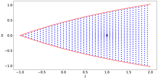
Figure 5: The blue dots are the joint eigenvalues of the spin-oscillator system in the region $-1\leq x\leq 2$ for $k=15$. The red line corresponds to the boundary of the image of the momentum map, and the black circle indicates the position of the focus-focus value.

The symplectic invariants of this system were computed in [2] using a convention that differs from the one we use here; this discrepancy has been fixed in [4]. In fact, these works extended the results from [76], in which the polygonal invariant, the height invariant and the linear coefficients of the Taylor series invariant were computed (with yet another convention). Firstly, the height invariant is

$$S_{0,0}=1$$

and the Taylor series invariant starts as

$$S=\frac{5\ln 2}{2\pi}\ Y+\frac{1}{8\pi}\ XY+\mathscr{O}(3);$$

here $\mathscr{O}(3)$ means cubic or higher order terms, to simplify notation. In other words,

$$[S_{1,0}]=0,\qquad S_{0,1}=\frac{5\ln 2}{2\pi},\qquad S_{2,0}=0,\qquad S_{1,1}=\frac{1}{8\pi},\qquad S_{0,2}=0.$$

Secondly, we can also infer the Taylor expansion of Eliasson’s function $f_{r}$ from [2, Lemma 4.1]; we illustrate this by obtaining this expansion up to $\mathscr{O}(3)$. The formula contained in this lemma says that if $(\xi_{1},\xi_{2})=(x_{1},f_{r}(x_{1},x_{2}))$ then

$$x_{2}=\frac{1}{2}\xi_{2}+\frac{1}{16}\xi_{1}\xi_{2}+\mathscr{O}(3).$$

This means that

$$\begin{split}\xi_{2}&=f_{r}\left(\xi_{1},\frac{1}{2}\xi_{2}+\frac{1}{16}\xi_{1}\xi_{2}+\mathscr{O}(3)\right)\\ &\begin{aligned} =f_{r}(0)+\partial_{x}f_{r}(0)\xi_{1}+\frac{\partial_{y}f_{r}(0)}{2}\xi_{2}+\frac{\partial^{2}_{x}f_{r}(0)}{2}\xi_{1}^{2}+\left(\frac{\partial_{y}f_{r}(0)}{16}+\frac{\partial_{x}\partial_{y}f_{r}(0)}{2}\right)\xi_{1}\xi_{2}\\ +\frac{\partial^{2}_{y}f_{r}(0)}{8}\xi_{2}^{2}+\mathscr{O}(3).\end{aligned}\end{split}$$

Hence we can identify the coefficients to find

$$\partial_{x}f_{r}(0)=0,\quad\partial_{y}f_{r}(0)=2,\quad\partial^{2}_{x}f_{r}(0)=0,\quad\partial_{x}\partial_{y}f_{r}(0)=-\frac{1}{4},\quad\partial^{2}_{y}f_{r}(0)=0,$$

and in particular $s(0)=0$. This reasoning could be used to compute higher order derivatives of $f_{r}$, but we will not need those in what follows.

Finally, a representative of the polygonal invariant corresponding to $\epsilon=+1$ and with vanishing twisting number is represented in Figure 6.

Figure 6: A representative of the privileged polygon for the spin-oscillator system.

We recover these invariants in the numerical simulations below. More precisely:

• we recover the height invariant in Figure 7,

• we recover $\partial_{x}f_{r}(0)$ in Figure 8 and $\partial_{y}f_{r}(0)$ in Figure 9 (and hence we obtain $s(0)$),

• we obtain a good labelling and recover the associated $\sigma_{1}(0)$ by using Formula (20) for a fixed regular value $c$ close to the focus-focus value and varying $k$ in Figure 11, and investigate the corresponding error term in Figure 12; recall that the integer part of $\sigma_{1}(0)$ gives the twisting number associated with the action variable selected by the labelling, while its fractional part gives the coefficient $[S_{1,0}]$ of the Taylor series invariant,

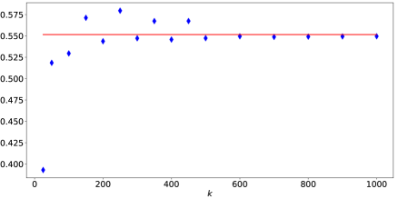
Figure 13: Determination of $S_{0,1}$ for the spin-oscillator system. The blue diamonds correspond to Formula (32) evaluated at $(j,\ell)=(0,0)$ and with $x=0.01$, for different values of $k$. The red line corresponds to the theoretical value $S_{0,1}=\frac{5\ln 2}{2\pi}$.

• we recover the coefficient $S_{0,1}$ of the Taylor series invariant using Proposition 6.8 in Figure 13,

• in Figure 14, we recover the privileged semitoric polygon thanks to Proposition 5.12 (see also Remark 4.30), using $\sigma_{1}(0)$ and Proposition 5.8,

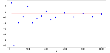
Figure 15: Determination of $\partial_{x}\partial_{y}f_{r}(0)$ for the spin-oscillator using Formula (56) with $x=0.01$ and $\lambda=1$, for different values of $k$. The red line corresponds to the theoretical result $\partial_{x}\partial_{y}f_{r}(0)=-\frac{1}{4}$.

• we recover the derivative $\partial_{x}\partial_{y}f_{r}(0)$ using Formula (56) below in Figure 15,

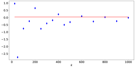
Figure 16: Determination of $S_{1,1}$ for the spin-oscillator using Formula (55) with $x=0.01$ and $\mu=1$, for different values of $k$. The red line corresponds to the theoretical result $S_{1,1}=\frac{1}{8\pi}$.

• finally, we recover the coefficient $S_{1,1}$ of the Taylor series invariant using Formula (55) below in Figure 16.

Remark 8.1 In view of our results and general strategy, some of the quantities that we recover from the joint spectrum should be obtained by first taking the limit $\hbar\to 0$ for a quantity defined at a regular value $c$ and then the limit $c\to(1,0)$ (recall that here $(1,0)$ is the focus-focus value). Hence for numerical purposes, it is important to fix some $c$ close to $(1,0)$ and let $\hbar$ vary for this given $c$. If instead one fixes a small value of $\hbar$ and lets $c$ vary, one could get less convincing results since it may happen that $\hbar$ should be taken smaller and smaller as $c$ becomes closer to the singular value. We illustrate this for the numerical computation of $\sigma_{1}(0)$ in Figure 10.   $\triangle$

We will illustrate part of the computation of higher order terms for Eliasson’s diffeomorphism and the Taylor series invariant in this example. Using the notation of Proposition 6.10 and the exact values of $\partial_{x}f_{r}(0)$, $\partial_{y}f_{r}(0)$, $S_{1,0}$, $S_{0,1}$, $\partial^{2}_{x}f_{r}(0)$, $\partial^{2}_{y}f_{r}(0)$, $S_{2,0}$ and $S_{0,2}$ in this precise example, we compute

$$d_{0}(\mu)=-\frac{\mu}{\pi},\qquad c_{0}(\mu)=-\frac{1}{2\pi}\arctan(2\mu)+\frac{5\mu\ln 2}{\pi}-\frac{\mu}{\pi}\ln(1+4\mu^{2}),$$

as well as

$$d_{1}(\mu)=-\frac{\mu}{\pi}\partial_{x}\partial_{y}f_{r}(0),\qquad c_{1}(\mu)=3\mu S_{1,1}+\mu\partial_{x}\partial_{y}f_{r}(0)\left(\frac{5\ln 2}{\pi}-\frac{1}{2\pi}-\frac{\ln(1+4\mu^{2})}{2\pi}\right).$$

This implies that

$$\partial_{x}\partial_{y}f_{r}(0)=-\frac{\pi}{\mu x\ln x}\left(g_{\mu}(x)+\frac{\mu}{\pi}\ln x+\frac{1}{2\pi}\arctan(2\mu)-\frac{5\mu\ln 2}{\pi}+\frac{\mu}{\pi}\ln(1+4\mu^{2})\right)\\ +\mathscr{O}\left(\frac{1}{\ln x}\right)$$

and that

$$S_{1,1}=\frac{1}{3}\left(\frac{c_{1}(\mu)}{\mu}-\partial_{x}\partial_{y}f_{r}(0)\left(\frac{5\ln 2}{\pi}-\frac{1}{2\pi}-\frac{\ln(1+4\mu^{2})}{2\pi}\right)\right)$$ (55)

where we can obtain $c_{1}(\mu)$ as

$$c_{1}(\mu)=\frac{1}{x}\left(g_{\mu}(x)+\frac{\mu}{\pi}\ln x+\frac{1}{2\pi}\arctan(2\mu)-\frac{5\mu\ln 2}{\pi}+\frac{\mu}{\pi}\ln(1+4\mu^{2})+\frac{\mu}{\pi}\partial_{x}\partial_{y}f_{r}(0)x\ln x\right)\\ +\mathscr{O}(x\ln x).$$

Hence if we already know all the above quantities and simply want to recover $\partial_{x}\partial_{y}f_{r}(0)$ and $S_{1,1}$, we can first obtain

$$\partial_{x}\partial_{y}f_{r}(0)=\lim_{x\to 0^{+}}\lim_{\hbar\to 0}\frac{-\pi\left(\frac{E_{j,\ell}-E_{j+1,\ell}+\mu\hbar}{E_{j,\ell+1}-E_{j,\ell}}+\frac{\mu}{\pi}\ln x+\frac{1}{2\pi}\arctan(2\mu)-\frac{5\mu\ln 2}{\pi}+\frac{\mu}{\pi}\ln(1+4\mu^{2})\right)}{\mu x\ln x}$$ (56)

thanks to Lemma 5.2 applied with $c=(x,\mu x)$ and then use it to recover $c_{1}(\mu)$ from the joint spectrum, and finally $S_{1,1}$ thanks to Formula (55). A similar formula as above for $S_{1,1}$ with a double limit can be obtained in a similar fashion.

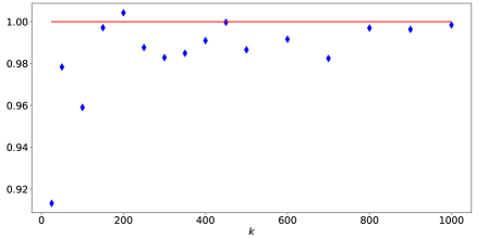
Figure 7: Determination of the height invariant for the spin-oscillator using Proposition 6.1. The blue diamonds correspond to $\frac{\hbar^{2-\delta}}{2c}N_{\hbar}(\delta,c,0)$ for $c=1$, $\delta=0.4$ and different values of $k=\hbar^{-1}$. The solid red line is the theoretical value $S_{0,0}=1$.

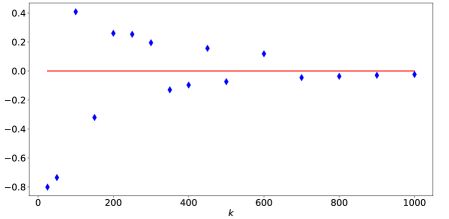
Figure 8: Determination of $\partial_{x}f_{r}(0)$ for the spin-oscillator using Formula (18) with $x=0.01$, $\mu=2$ and $(j_{1},\ell_{1})=(0,0)=(j_{2},\ell_{2})$, for different values of $k$. The red line corresponds to the theoretical result $\partial_{x}f_{r}(0)=0$.

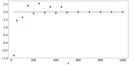
Figure 9: Determination of $\partial_{y}f_{r}(0)$ for the spin-oscillator using Formula (19) with $x=0.01$, $\mu=2$ and $(j_{1},\ell_{1})=(0,0)=(j_{2},\ell_{2})$, for different values of $k$. The red line corresponds to the theoretical result $\partial_{y}f_{r}(0)=2$.

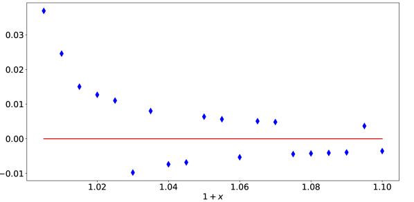
(a) $k=250$.

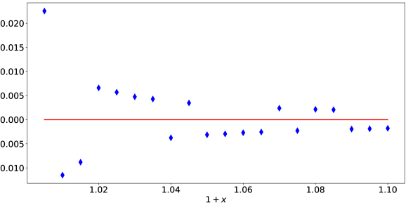
(b) $k=500$.

Figure 10: Determination of $\sigma_{1}^{\text{p}}(0)$ for the spin-oscillator system. The blue diamonds correspond to Formula (20) evaluated at $(j,\ell)=(0,0)$ for a given $k$ and different values of $x$. The red line corresponds to the theoretical value $\sigma_{1}^{\text{p}}(0)=0$.

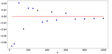
Figure 11: Determination of $\sigma_{1}^{\textup{p}}(0)$ for the spin-oscillator system. The blue diamonds correspond to Formula (20) evaluated at $(j,\ell)=(0,0)$ with $x=0.01$, for different values of $k$. The red line corresponds to the theoretical value $\sigma_{1}^{\textup{p}}(0)=0$. Since the value of the invariant is integer, this is an example where the twisting number is unstable.

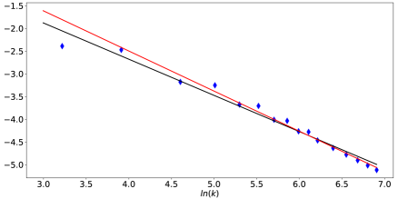
Figure 12: Error in the determination of $\sigma_{1}^{\textup{p}}(0)$ for the spin-oscillator system. The blue diamonds correspond to the logarithm of the error between Formula (20) evaluated at $(j,\ell)=(0,0)$ and $\sigma_{1}^{\textup{p}}(0)$ with $x=0.01$, for different values of $\ln k$. In black, the line of linear regression; in red, the line of linear regression computed after discarding the first two points.

8.2 Coupled angular momenta

The other system that we use to illustrate our results was introduced in [84] and consists in coupling two classical spins in a non-trivial way. More precisely, let $R_{2}>R_{1}>0$ and endow $\mathbb{S}^{2}\times\mathbb{S}^{2}$ with the symplectic form $\omega=-(R_{1}\omega_{\mathbb{S}^{2}}\oplus R_{2}\omega_{\mathbb{S}^{2}})$ and coordinates $(x_{1},y_{1},z_{1}),(x_{2},y_{2},z_{2})$. We consider the momentum map:

$$F=(J,H),\qquad J=R_{1}z_{1}+R_{2}z_{2},\qquad H=(1-t)z_{1}+t(x_{1}x_{2}+y_{1}y_{2}+z_{1}z_{2})$$

depending on a parameter $t\in[0,1]$. This system is semitoric with exactly one focus-focus singularity for $t$ chosen in a certain interval depending on $R_{1}$ and $R_{2}$, always containing $t=\frac{1}{2}$, see [60].

For quantization purposes, we ask that $R_{1}$ and $R_{2}$ are half-integers. Using the quantization of the sphere described in the previous example, we obtain the Hilbert spaces $\mathcal{H}_{k}\simeq\mathbb{C}_{\leq 2kR_{1}-1}[z]\otimes\mathbb{C}_{\leq 2kR_{2}-1}[w]$ with inner product

$$\langle P_{1}\otimes P_{2},Q_{1}\otimes Q_{2}\rangle_{k}=\left(\int_{\mathbb{C}}\frac{P_{1}(z)\overline{Q_{1}(z)}}{(1+|z|^{2})^{2kR_{1}+1}}|dz\wedge d\bar{z}|\right)\left(\int_{\mathbb{C}}\frac{P_{2}(w)\overline{Q_{2}(w)}}{(1+|w|^{2})^{2kR_{2}+1}}|dw\wedge d\bar{w}|\right).$$

Furthermore, $J$ and $H$ are quantized as the Berezin-Toeplitz operators

$$\begin{cases}\hat{J}_{k}=\frac{1}{2k}\left((1+2kR_{1})\hat{Z}_{kR_{1}}\otimes\mathrm{Id}+(1+2kR_{2})\mathrm{Id}\otimes\hat{Z}_{kR_{2}}\right),\\[5.69054pt] \begin{aligned} \hat{H}_{k}&=\frac{(1-t)}{2kR_{1}}(1+2kR_{1})\hat{Z}_{kR_{1}}\otimes\mathrm{Id}\\ &+\frac{t(1+2kR_{1})(1+2kR_{2})}{4k^{2}R_{1}R_{2}}\left(\hat{X}_{kR_{1}}\otimes\hat{X}_{kR_{2}}+\hat{Y}_{kR_{1}}\otimes\hat{Y}_{kR_{2}}+\hat{Z}_{kR_{1}}\otimes\hat{Z}_{kR_{2}}\right).\end{aligned}\end{cases}$$

with $\hat{X},\hat{Y},\hat{Z}$ as in Equation (54). More details can be found in [60, Section 4], including the computation of the joint spectrum of $(\hat{J}_{k},\hat{H}_{k})$, which is displayed in Figure 17.

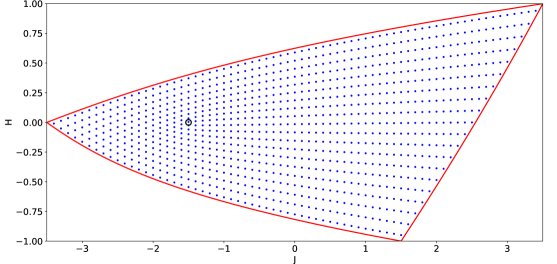
Figure 17: The blue dots are the joint eigenvalues of the quantum coupled angular momenta with $R_{1}=1$, $R_{2}=\frac{5}{2}$ and $t=\frac{1}{2}$ for $k=10$. The red line corresponds to the boundary of the image of the momentum map, and the black circle indicates the focus-focus value.

The symplectic invariants were computed in [1] for all values of $R_{1},R_{2}$ and $t$. Here we choose $R_{1}=1$, $R_{2}=\frac{5}{2}$ and $t=\frac{1}{2}$ for our numerical simulations (part of the invariants were computed for these precises values of the parameters in [60]). In this case, the height invariant is

$$S_{0,0}=2+\frac{1}{\pi}\left(3-5\arctan\left(\frac{3}{4}\right)-2\arctan 3\right),$$ (57)

the Taylor series invariant reads

$$S=\frac{1}{2\pi}\arctan\left(\frac{13}{9}\right)X+\frac{1}{2\pi}\left(\frac{7}{2}\ln 2+3\ln 3-\frac{3}{2}\ln 5\right)Y+\mathscr{O}(2)$$

and the first order derivatives of Eliasson’s diffeomorphism are

$$\partial_{x}f_{r}(0)=-\frac{1}{3},\qquad\partial_{y}f_{r}(0)=\frac{10}{3}.$$

Moreover, a representative of the polygonal invariant with vanishing twisting number and $\epsilon=+1$ is displayed in Figure 18.

Figure 18: A representative of the privileged polygon for the coupled angular momenta system.

As in the previous example,

• we recover the height invariant in Figure 19,

• we recover $\partial_{x}f_{r}(0)$ in Figure 20 and $\partial_{y}f_{r}(0)$ in Figure 21 (and hence we obtain $s(0)$),

• we recover $\sigma_{1}^{\textup{p}}(0)$ by using Formula (20) for a fixed small value of $x$ and various $k$ in Figure 22,

• we recover the coefficient $S_{0,1}$ of the Taylor series invariant using formula Proposition 6.8 in Figure 23,

• in Figure 26, we recover the privileged semitoric polygon thanks to Proposition 5.12.

In principle, we could also recover the higher order terms for the Taylor series invariants as in the previous example, but in this case the computations are more involved. In Figure 24, we illustrate Remark 5.13 by recovering the Duistermaat-Heckman function of $J$ from the joint spectrum. We also illustrate the detection of focus-focus values in Figure 25.

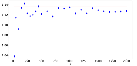
Figure 19: Determination of the height invariant for the coupled angular momenta using Proposition 6.1. The blue diamonds correspond to $\frac{\hbar^{2-\delta}}{2c}N_{\hbar}(\delta,c,0)$ for $c=1$, $\delta=0.4$ and different values of $k=\hbar^{-1}$. The solid red line is the theoretical value given in Equation (57).

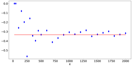
Figure 20: Determination of $\partial_{x}f_{r}(0)$ for the coupled angular momenta system using Formula (18) with $x=0.01$, $\mu=2$ and $(j_{1},\ell_{1})=(0,0)=(j_{2},\ell_{2})$, for different values of $x$. The red line corresponds to the theoretical result $\partial_{x}f_{r}(0)=-\frac{1}{3}$.

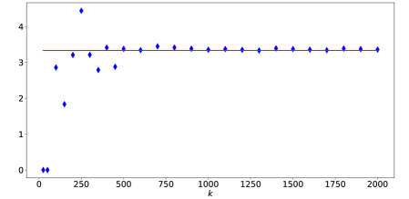
Figure 21: Determination of $\partial_{y}f_{r}(0)$ for the coupled angular momenta system using Formula (19) with $x=0.01$, $\mu=2$ and $(j_{1},\ell_{1})=(0,0)=(j_{2},\ell_{2})$, for different values of $k$. The red line corresponds to the theoretical result $\partial_{y}f_{r}(0)=\frac{10}{3}$.

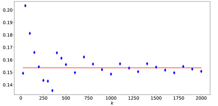
Figure 22: Determination of $\sigma_{1}^{\textup{p}}(0)$ for the coupled angular momenta system. The blue diamonds correspond to Formula (20) evaluated at $(j,\ell)=(0,0)$ with $x=0.01$, for different values of $k$. The red line corresponds to $\sigma_{1}^{\textup{p}}(0)=\frac{1}{2\pi}\arctan(\frac{13}{9})$.

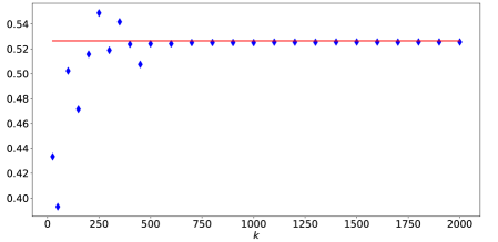
Figure 23: Determination of $S_{0,1}$ for the coupled angular momenta system. The blue diamonds correspond to Formula (32) evaluated at $(j,\ell)=(0,0)$ with $x=0.01$, for different values of $k$. The red line corresponds to the theoretical value $S_{0,1}=\frac{1}{2\pi}\left(\frac{7}{2}\ln 2+3\ln 3-\frac{3}{2}\ln 5\right)$.

Figure 24: Determination of the Duistermaat-Heckman function $\rho_{J}$ for the coupled angular momenta system using Equation (22); the blue dots represent the left hand side of this equation, with $k=200$, $\delta=\frac{1}{4}$ and $c=1$. The solid red line is the graph of $\rho_{J}$, which can be computed explicitly, for instance thanks to the polygon in Figure 18.

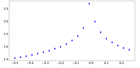
Figure 25: Computation of the inverse level spacings $\frac{\hbar}{E_{0,1}-E_{0,0}}$ related to the function $a_{2}(c)$, see Lemma 5.2, where $c=(-1.5,y)$ for various values of $y$; here $k=50$. Notice the peak indicating the position of the focus-focus critical value at $y=0$.

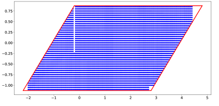
Figure 26: Determination of the privileged polygon for the coupled angular momenta system using Proposition 5.12; the blue dots represent the set $\Delta_{\hbar}(\mathcal{K}(S,\mathcal{U}))$ where $S=\{(x,y)\in\mathbb{R}^{2}\ |\ -3.3\leq x\leq 3.1\}$ for $k=20$, while the solid red lines represent a translation of the privileged semitoric polygon shown in Figure 18.

Appendix A Semiclassical operators

In this section, we gather the definition and properties of semiclassical operators that are used throughout the paper. We allow $\hbar$-pseudodifferential operators as well as Berezin-Toeplitz operators. When quantizing $T^{*}\mathbb{R}^{d}=\mathbb{C}^{d}$, these two notions are related through the Bargmann transform; we also state some useful properties of this transform.

A.1 Pseudodifferential operators

Let $X=\mathbb{R}^{d}$ or let $X$ be a compact Riemannian manifold. We consider $\hbar$-pseudodifferential operators acting on the (fixed) Hilbert space $\mathcal{H}_{\hbar}=L^{2}(X)$ with usual inner product, and $\hbar$ is a continuous parameter taking its values in an interval of the form $(0,\hbar_{0}]$ for some $\hbar_{0}>0$. In order to define these operators, we need to separate the two cases.

If $X=\mathbb{R}^{d}$ (hence $T^{*}X\simeq\mathbb{R}^{2d}$), we say that $A_{\hbar}$ is an $\hbar$-pseudodifferential operator if it is the Weyl quantization of a symbol $a\in S(m)$ where $m$ is some order function (as in [101, Section 4], for instance): $m$ is a measurable function such that there exist constants $C,N>0$ so that

$$\forall U,V\in\mathbb{R}^{2d}\qquad 1\leq m(U)\leq C\langle V-U\rangle^{N}m(V)$$

where $\langle U\rangle=\left(1+\|U\|^{2}\right)^{\frac{1}{2}}$. Some usual choices are $m(U)=\langle U\rangle^{\mu}$ or $m(x,\xi)=\langle\xi\rangle^{\mu}$ for some $\mu\in\mathbb{R}$. Let $a=a(\cdot,\hbar)$ be a family of elements of $C^{\infty}(\mathbb{R}^{2d})$; we say that $a$ belongs to $S(m)$ if

$$\forall\alpha\in\mathbb{N}^{2d}\quad\exists C_{\alpha}>0\quad\forall\hbar\in(0,\hbar_{0}]\quad\forall(x,\xi)\in\mathbb{R}^{2d}\qquad|\partial^{\alpha}a(x,\xi,\hbar)|\leq C_{\alpha}m(x,\xi).$$

We will always assume that $a\in S(m)$ is asymptotic to $\sum_{j\geq 0}\hbar^{j}a_{j}$, where for every $j\geq 0$, $a_{j}\in C^{\infty}(\mathbb{R}^{2d})$ is independent of $\hbar$, in the sense that

$$\forall N\geq 1\qquad a-\sum_{j=0}^{N}\hbar^{j}a_{j}\in\hbar^{N+1}S(m).$$

If it is not identically zero, the function $a_{0}$ is called the principal symbol of $A_{\hbar}$. The Weyl quantization $A_{\hbar}=\mathrm{Op}_{\hbar}^{W}(a)$ of $a\in S(m)$ is defined by the following formula: for every $u\in\mathscr{S}(\mathbb{R}^{d})$ and for every $x\in\mathbb{R}^{d}$,

$$(A_{\hbar}u)(x)=\frac{1}{(2\pi\hbar)^{d}}\int_{\mathbb{R}^{d}}\int_{\mathbb{R}^{d}}e^{\frac{i}{\hbar}\langle x-y,\xi\rangle}a\left(\frac{x+y}{2},\xi\right)u(y)\operatorname{d}\!{y}\operatorname{d}\!{\xi}.$$

By a slight abuse of notation, we say that $A_{\hbar}$ belongs to $S(m)$ when $a$ does.

If $X$ is a compact Riemannian manifold, we always work with the order function given in local coordinates by $m(x,\xi)=\langle\xi\rangle^{\mu}$ for some $\mu\in\mathbb{R}$; we say that $A_{\hbar}$ is an $\hbar$-pseudodifferential operator in the Kohn-Nirenberg class $S(m)$ if in local coordinates, after a cut-off in $x\in X$, $A_{\hbar}$ can be written as an $\hbar$-pseudodifferential operator with symbol $a\in S(m)$. This does not depend on the choice of local coordinates. See for instance [101, Section 14.2] for more details.

We need two notions of ellipticity. Firstly, we say that $A_{\hbar}\in S(m)$ is elliptic at $p\in T^{*}X$ if its principal symbol does not vanish at $p$. Secondly, we say that $A_{\hbar}\in S(m)$ is elliptic at infinity in $S(m)$ if there exists $C>0$ such that $|a_{0}|\geq Cm$ outside of a compact set.

Additionally, we will need to consider families of elements of $L^{2}(X)$ upon which $\hbar$-pseudodifferential operators act (for instance, families of eigenvectors of such an operator), and to study their localization in phase space.

Definition A.1

Let $(u_{\hbar})_{\hbar\in\mathcal{I}}$ be a sequence of elements of $\mathscr{D}^{\prime}(\mathbb{R}^{d})$, and let $p\in T^{*}X$. We say that

• $(u_{\hbar})$ is admissible if for any $\hbar$-pseudodifferential operator $A_{\hbar}$ with compactly supported Weyl symbol, there exists $N\in\mathbb{Z}$ such that $\|A_{\hbar}u_{\hbar}\|_{L^{2}(\mathbb{R}^{d})}=\mathscr{O}(\hbar^{N})$;

• the admissible sequence $(u_{\hbar})$ is negligible at $p$ if there exists an $\hbar$-pseudodifferential operator $A_{\hbar}$, elliptic at $p$, such that $\|A_{\hbar}u_{\hbar}\|_{L^{2}(\mathbb{R}^{d})}=\mathscr{O}(\hbar^{\infty})$;

• $p\notin\mathrm{WF}(u_{\hbar})$ if and only if $(u_{\hbar})$ is negligible at $p$. The set $\mathrm{WF}(u_{\hbar})\subset T^{*}X$ is called the wavefront set of $(u_{\hbar})$.

When looking for eigenvalues of a semiclassical operator, it is often useful to consider functions that solve the eigenvalue equation “locally in phase space” in the following sense.

Definition A.2

Let $A_{\hbar}$ be an $\hbar$-pseudodifferential operator. A microlocal solution to the equation $A_{\hbar}u_{\hbar}=\mathscr{O}(\hbar^{\infty})$ over the open set $\mathcal{U}$ is an admissible family $(u_{\hbar})_{\hbar\in\mathcal{I}}$ of elements of $\mathcal{H}_{\hbar}$ such that $\mathrm{WF}(A_{\hbar}u_{\hbar})\cap\mathcal{U}=\emptyset$.

By adapting the above definitions, one can compare the action of operators on a given part of the phase space.

Definition A.3

Let $A_{\hbar},B_{\hbar}$ be two $\hbar$-pseudodifferential operators. We say that

• $A_{\hbar}$ is negligible at $p\in T^{*}X$ if there exists an $\hbar$-pseudodifferential operator $P_{\hbar}$, elliptic at $p$, such that $\|P_{\hbar}A_{\hbar}\|=\mathscr{O}(\hbar^{\infty})$,

• $A_{\hbar}$ and $B_{\hbar}$ are microlocally equivalent at $p$ if and only if $A_{\hbar}-B_{\hbar}$ is negligible at $p$. In this case we write $A_{\hbar}\sim B_{\hbar}$ at $p$,

• $A_{\hbar}$ and $B_{\hbar}$ are microlocally equivalent on the open set $\mathcal{U}\subset T^{*}X$ if and only if they are microlocally equivalent at every point of $\mathcal{U}$.

Finally, we use the notation $\mathbb{C}_{\hbar}$ for the ring of constant symbols, that can be seen as symbols in $S(1)$ on $\{0\}$.

A.2 Berezin-Toeplitz operators

On a compact phase space.

We now consider a compact symplectic manifold $(M,\omega)$. In fact, we shall always assume that $(M,\omega)$ is Kähler; this is not really restrictive for the purpose of the present paper, since:

• a compact symplectic four-dimensional manifold endowed with a Hamiltonian $\mathbb{S}^{1}$-action (which is the case if there exists a semitoric system on $M$) is automatically Kähler by [54, Theorem 7.1] (see case (M2) in Section 3),

• a compact symplectic surface is automatically Kähler (see case (M3) in Section 3).

Furthermore, we will always assume that $M$ is quantizable in the sense that the cohomology class $\left[\frac{\omega}{2\pi}\right]$ is integral; this amounts to the existence of a Hermitian and holomorphic line bundle $(\mathscr{L},h_{\mathscr{L}})\to M$ whose Chern connection $\nabla$ has curvature $-i\omega$, called prequantum line bundle.

In this context, we consider Berezin-Toeplitz operators [9, 13, 12, 16, 64], which act on a sequence of finite-dimensional Hilbert spaces defined as follows. Let $(\mathscr{K},h_{\mathscr{K}})\to M$ be another Hermitian holomorphic complex line bundle; for instance one can choose $\mathscr{K}=\delta$ a half-form bundle (a square root of the canonical bundle) when it exists, to obtain the so-called metaplectic correction. For any integer $k\geq 1$, $h_{\mathscr{L}}$ and $h_{\mathscr{K}}$ induce a Hermitian form $h_{k}$ on $\mathscr{L}^{\otimes k}\otimes\mathscr{K}$, and we consider the Hilbert space

$$\mathcal{H}_{k}=H^{0}(M,\mathscr{L}^{\otimes k}\otimes\mathscr{K}),\qquad\langle\phi,\psi\rangle_{k}=\int_{M}h_{k}(\phi,\psi)\left|\frac{\omega^{\wedge n}}{n!}\right|$$

of holomorphic sections of the line bundle $\mathscr{L}^{\otimes k}\otimes\mathscr{K}\to M$. The semiclassical parameter in this context is $\hbar=k^{-1}$ and takes only discrete values. A Berezin-Toeplitz operator is an operator of the form

$$T_{k}=\Pi_{k}f(\cdot,k)\Pi_{k}+R_{k}:\mathcal{H}_{k}\to\mathcal{H}_{k}$$

where $\Pi_{k}:L^{2}(M,\mathscr{L}^{\otimes k}\otimes\mathscr{K})\to\mathcal{H}_{k}$ is the orthogonal projector from the space of square integrable sections to the space of holomorphic sections of $\mathscr{L}^{\otimes k}\otimes\mathscr{K}\to M$, $f(\cdot,k)$ is a sequence of elements of $C^{\infty}(M)$ with an asymptotic expansion of the form $f(\cdot,k)=\sum_{\ell\geq 0}k^{-\ell}f_{\ell}$ in the $C^{\infty}$-topology and $R_{k}$ is a sequence of operators whose norm is $\mathscr{O}(k^{-N})$ for every $N\geq 1$. If not identically zero, the term $f_{0}$ in the above asymptotic expansion is called the principal symbol of $T_{k}$. When $R_{k}=0$, we simply write $T_{k}(f(\cdot,k))$ for $\Pi_{k}f(\cdot,k)\Pi_{k}$.

As before, we need to discuss the localization of sequences of sections in phase space in the semiclassical limit.

Definition A.4

Let $(\psi_{k})_{k\geq 1}$ be a sequence such that for each $k$, $\psi_{k}\in C^{\infty}(M,\mathscr{L}^{\otimes k}\otimes\mathscr{K})$, and let $m\in M$. We say that

• $(\psi_{k})$ is admissible if for every integer $\ell\geq 0$, for any vector fields $X_{1},\ldots,X_{\ell}$ on $M$ and for every compact set $C\subset M$, there exist a constant $c>0$ and an integer $N$ such that

  $$\forall p\in C\qquad|\nabla_{X_{1}}\ldots\nabla_{X_{\ell}}\psi_{k}(p)|\leq ck^{N}$$

  (here $|\cdot|$ stands for the pointwise norm given by the Hermitian metric on $\mathscr{L}^{\otimes k}\otimes\mathscr{K}$),

• the admissible sequence $(\psi_{k})$ is negligible at $m$ if there exists a neighborhood $\mathcal{V}$ of $m$ such that for any integers $\ell,N\geq 0$ and for any vector fields $X_{1},\ldots,X_{\ell}$ on $M$,

  $$\sup_{\mathcal{V}}|\nabla_{X_{1}}\ldots\nabla_{X_{\ell}}\psi_{k}|=\mathscr{O}(k^{-N}),$$

• $m\notin\mathrm{MS}(\psi_{k})$ if and only if $(\psi_{k})$ is negligible at $m$. The set $\mathrm{MS}(\psi_{k})$ is called the microsupport of $(\psi_{k})$.

Naturally, the microsupport is the analogue of the wavefront set, see Section A.3. We can then define negligibility and microlocal equality for Berezin-Toeplitz operators by applying these definitions to their Schwartz kernels, which are sections of $(\mathscr{L}^{\otimes k}\otimes\mathscr{K})\boxtimes(\overline{\mathscr{L}}^{\otimes k}\otimes\overline{\mathscr{K}})\to M\times\overline{M}$. Here $\overline{M}$ is $M$ endowed with the opposite symplectic and complex structures, and the external tensor product $\mathscr{L}\boxtimes\mathscr{L}^{\prime}$ of two line bundles $\mathscr{L}\to M$ and $\mathscr{L}^{\prime}\to M^{\prime}$ is the line bundle $\pi_{1}^{*}\mathscr{L}\otimes\pi_{2}^{*}\mathscr{L}^{\prime}$ where $\pi_{1}:M\times M^{\prime}\to M$ and $\pi_{2}:M\times M^{\prime}\to M^{\prime}$ are the natural projections.

We also need to define microlocal solutions in this context; however, there is a subtlety that did not appear in the $\hbar$-pseudodifferential case. Indeed, one would like to be able to consider a holomorphic section $\psi_{k}$ and to multiply it by a compactly supported smooth function, but the resulting section will not be holomorphic in general. This leads to the following definition (see also [58, Section 4]).

Definition A.5

Let $T_{k}$ be a Berezin-Toeplitz operator and let $\mathcal{U}\subset M$ be an open set. A microlocal solution to the equation $T_{k}u_{k}=\mathscr{O}(k^{-\infty})$ over $\mathcal{U}$ is an admissible sequence $(u_{k})_{k\geq 1}$ of elements of $C^{\infty}(\mathcal{U},\mathscr{L}^{\otimes k}\otimes\mathscr{K})$ such that for every $m\in\mathcal{U}$, there exists a function $\chi\in C^{\infty}(M)$, equal to one near $m$, and compactly supported in $\mathcal{U}$, such that

$$\Pi_{k}(\chi u_{k})=u_{k}+\mathscr{O}(k^{-\infty}),\qquad T_{k}(\Pi_{k}(\chi u_{k}))=\mathscr{O}(k^{-\infty})$$

near $m$.

On $\mathbb{C}^{d}$ or $\mathbb{C}^{d}\times M$ with $M$ compact.

We also need to consider Berezin-Toeplitz operators with symbols defined on $(\mathbb{R}^{2d},\omega_{0}=\operatorname{d}\!{\xi}_{1}\wedge\operatorname{d}\!{x}_{1}+\ldots+\operatorname{d}\!{\xi}_{d}\wedge\operatorname{d}\!{x}_{d})$, and in this context we have to to introduce some good symbol classes as in the previous section. More precisely, we identify $\mathbb{R}^{2d}$ with $\mathbb{C}^{d}$ using the complex coordinates $z_{j}=\frac{1}{\sqrt{2}}(x_{j}-i\xi_{j})$, and endow it with the line bundle $\mathscr{L}_{0}=\mathbb{C}^{d}\otimes\mathbb{C}\to\mathbb{C}^{d}$ equipped with its natural Hermitian form $h$, the connection $\nabla=\operatorname{d}\!{-}i\alpha$ where

$$\alpha=\frac{i}{2}\left(z_{1}\operatorname{d}\!{\bar{z}_{1}}+\ldots+z_{d}\operatorname{d}\!{\bar{z}_{d}}-\bar{z}_{1}\operatorname{d}\!{z}_{1}-\ldots-\bar{z}_{d}\operatorname{d}\!{z}_{d}\right)$$

and the unique holomorphic structure compatible with both $h$ and $\nabla$. We consider the quantum spaces $\mathcal{B}_{k}(\mathbb{C}^{d})=H^{0}(\mathbb{C}^{d},\mathscr{L}_{0}^{\otimes k})\cap L^{2}(\mathbb{C}^{d},\mathscr{L}_{0}^{\otimes k})$, that is

$$\mathcal{B}_{k}(\mathbb{C}^{d})=\bigg{\{}f\psi^{k}\quad|\quad f:\mathbb{C}^{d}\to\mathbb{C}\text{ holomorphic},\\ \left.\int_{\mathbb{C}^{d}}|f(z)|^{2}\exp(-k\|z\|^{2})\ \left|\operatorname{d}\!{z_{1}}\wedge\operatorname{d}\!{\bar{z}_{1}}\wedge\ldots\wedge\operatorname{d}\!{z_{d}}\wedge\operatorname{d}\!{\bar{z}_{d}}\right|<+\infty\right\}$$ (58)

for $k\geq 1$, where $\psi(z)=\exp\left(-\frac{1}{2}\|z\|^{2}\right)$ with $\|z\|^{2}=|z_{1}|^{2}+\ldots+|z_{d}|^{2}$. These spaces are called Bargmann spaces and are known to be Hilbert spaces [8] when equipped with the inner product

$$\langle f\psi^{k},g\psi^{k}\rangle_{k}=\int_{\mathbb{C}^{d}}f(z)\overline{g(z)}\exp(-k\|z\|^{2})\ \left|\operatorname{d}\!{z_{1}}\wedge\operatorname{d}\!{\bar{z}_{1}}\wedge\ldots\wedge\operatorname{d}\!{z_{d}}\wedge\operatorname{d}\!{\bar{z}_{d}}\right|.$$

The symbol classes that we will consider were discussed in [57, Section 3.3] and are very similar to the ones used for $\hbar$-pseudodifferential operators. Similarly to the previous section, we set $\langle z\rangle=(1+\|z\|^{2})^{\frac{1}{2}}$ and for $\mu\in\mathbb{R}$, we consider the weight function $m(z)=\langle z\rangle^{\mu}$. Then we say that $a(\cdot,k)$ belongs to the symbol class $S(m)$ if

$$\forall\alpha,\beta\in\mathbb{N}^{d}\quad\exists C_{\alpha,\beta}>0\quad\forall k\geq 1\quad\forall z\in\mathbb{C}^{d}\qquad|\partial^{\alpha}_{z}\partial^{\beta}_{\bar{z}}a(z,k)|\leq C_{\alpha,\beta}m(z).$$

We will assume as in the previous section that $a\in S(m)$ is asymptotic to $\sum_{j\geq 0}k^{-j}a_{j}$, where for every $j\geq 0$, $a_{j}\in C^{\infty}(\mathbb{C}^{d})$ is independent of $k$, in the sense that

$$\forall N\geq 1\qquad a-\sum_{j=0}^{N}k^{-j}a_{j}\in k^{-(N+1)}S(m).$$

A Berezin-Toeplitz operator in the class $S(m)$ is an operator of the form

$$A_{k}=\Pi_{k}a(\cdot,k)\Pi_{k}+S_{k}:\mathcal{B}_{k}(\mathbb{C}^{d})\to\mathcal{B}_{k}(\mathbb{C}^{d})$$

where $\Pi_{k}$ is the orthogonal projector $\Pi_{k}:L^{2}(\mathbb{C}^{d},\mathscr{L}^{\otimes k})\to\mathcal{B}_{k}(\mathbb{C}^{d})$ and $S_{k}:\mathcal{B}_{k}(\mathbb{C}^{d})\to\mathcal{B}_{k}(\mathbb{C}^{d})$ is an operator whose Schwartz kernel is of the form

$$S_{k}(z,w)=R_{k}(z,w)\exp(-Ck\|z-w\|^{2})$$

where $C>0$ does not depend on $k$ and $R_{k}$ is a negligible sequence of sections of $C^{\infty}(\mathbb{C}^{d}\times\mathbb{C}^{d},\mathcal{L}_{0}^{\otimes k}\boxtimes\overline{\mathcal{L}_{0}}^{\otimes k})$. Here the definition of negligible is the same as in A.4.

The notions of ellipticity and ellipticity at infinity can be defined as in the previous section. The notions of admissibility, negligibility and microsupport can be defined as in Definition A.4, and one can reformulate them in a similar fashion as Definition A.1; for instance, one can check that $(\psi_{k})$ is negligible at $z_{0}\in\mathbb{C}^{d}$ if and only if there exists a Berezin-Toeplitz operator $T_{k}$, elliptic at $z_{0}$, such that $\|T_{k}\psi_{k}\|_{k}=\mathscr{O}(k^{-\infty})$ (see [58, Lemma 2.7]). Finally, one can define microlocal solutions as in Definition A.5.

Finally, we will need to handle phase spaces of the form $\mathbb{C}^{d}\times M$ where $M$ is a quantizable compact Kähler manifold (see case (M3)). In order to do so, we consider the same line bundle $\mathscr{L}_{0}\to\mathbb{C}^{d}$ as above and a prequantum line bundle $\mathscr{L}\to M$ and auxiliary Hermitian line bundle $\mathscr{K}\to M$. Then the quantum Hilbert spaces are

$$\mathcal{H}_{k}:=H^{0}(\mathbb{C}^{d}\times M,\mathscr{L}_{0}^{k}\boxtimes(\mathscr{L}^{k}\otimes\mathscr{K}))\cap L^{2}(\mathbb{C}^{d}\times M,\mathscr{L}_{0}^{k}\boxtimes\mathscr{L}^{k}\otimes\mathscr{K})$$

endowed with the inner product obtained by the same construction as in the compact case, using the Hermitian metric induced on $\mathscr{L}_{0}^{k}\boxtimes(\mathscr{L}^{k}\otimes\mathscr{K})$ by those of $\mathscr{L}_{0}$, $\mathscr{L}$ and $\mathscr{K}$. In fact, one readily checks that $\mathcal{H}_{k}\simeq\mathcal{B}_{k}(\mathbb{C}^{d})\otimes H^{0}(N,\mathscr{L}^{k}\otimes\mathscr{K})$ as Hilbert spaces. There is no specific difficulty with this setting: one can work with symbol classes that are similar to the case of $\mathbb{C}^{d}$ in order to handle the lack of compactness on the first factor. The notions of ellipticity, ellipticity at infinity, admissibility, negligibility and microsupport are still well-defined.

A.3 The Bargmann transform

The semiclassical Bargmann transform is the linear map $B_{k}:L^{2}(\mathbb{R}^{d})\to\mathcal{B}_{k}(\mathbb{C}^{d})$ given by the following formula: for every $f\in L^{2}(\mathbb{R}^{d})$ and for every $z\in\mathbb{C}^{d}$,

$$(B_{k}f)(z)=2^{\frac{d}{4}}\left(\frac{k}{2\pi}\right)^{\frac{3d}{4}}\left(\int_{\mathbb{R}^{d}}e^{-\frac{k}{2}\left(z^{2}+x^{2}-2\sqrt{2}z\cdot x\right)}f(x)\operatorname{d}\!{x}\right)\psi^{k}(z)$$

where $z^{2}=z_{1}^{2}+\ldots+z_{n}^{2}$, $x^{2}=x_{1}^{2}+\ldots+x_{n}^{2}$ and $z\cdot x=z_{1}x_{1}+\ldots+z_{n}x_{n}$. It is a unitary operator between those two Hilbert spaces, and has the following semiclassical properties, see for instance [101, Sections 13.3 and 13.4] for a class of symbols with bounded derivatives, or [58, Section 3] for the $d=1$ case (the general case being completely similar):

1. if $(u_{k})_{k\geq 1}$ is an admissible sequence of elements of $\mathscr{S}(\mathbb{R})$, then $(x_{1},\ldots,x_{d},\xi_{1},\ldots,\xi_{d})\notin\mathrm{WF}(u_{k})$ if and only if $\phi(x_{1},\ldots,x_{d},\xi_{1},\ldots,\xi_{d})\notin\mathrm{MS}(B_{k}u_{k})$ (in other words, the notions of wavefront set and microsupport are equivalent via the semiclassical Bargmann transform),

2. if $a(.,k)$ belongs to the class $S(m)$ where $m(z)=\langle z\rangle^{\mu}$ for some $\mu\in\mathbb{R}$, then $B_{k}^{*}T_{k}(a(\cdot,k))B_{k}$ is a pseudodifferential operator in $S(m\circ\phi)$ with principal symbol $a_{0}\circ\phi$.

Here $\phi$ is defined as $\phi(x_{1},\ldots,x_{d},\xi_{1},\ldots,\xi_{d})=\frac{1}{\sqrt{2}}(x_{1}-i\xi_{1},\ldots,x_{d}-i\xi_{d})$. To understand these properties, one can think of the semiclassical Bargmann transform as a Fourier integral operator associated with the symplectomorphism $\phi^{-1}:\mathbb{C}^{d}\to\mathbb{R}^{2d}$.

References

- [1] J. Alonso, H. R. Dullin, and S. Hohloch. Symplectic classification of coupled angular momenta. Nonlinearity, 33(1):417–468, Dec 2019.
- [2] J. Alonso, H. R. Dullin, and S. Hohloch. Taylor series and twisting-index invariants of coupled spin-oscillators. J. Geom. Phys., 140:131–151, 2019.
- [3] J. Alonso and S. Hohloch. Survey on recent developments in semitoric systems. RIMS Kokyuroku, 2137, 2019.
- [4] J. Alonso i Fernández. On the symplectic invariants of semitoric systems. PhD thesis, Universiteit Antwerpen, 2019.
- [5] M. F. Atiyah. Convexity and commuting Hamiltonians. Bull. London Math. Soc., 14(1):1–15, 1982.
- [6] O. Babelon, L. Cantini, and B. Douçot. A semi-classical study of the Jaynes-Cummings model. J. Stat. Mech. Theory Exp., 7:P07011, 45, 2009.
- [7] O. Babelon and B. Douçot. Higher index focus–focus singularities in the Jaynes–Cummings–Gaudin model: Symplectic invariants and monodromy. Journal of Geometry and Physics, 87:3–29, 2015. Finite dimensional integrable systems: on the crossroad of algebra, geometry and physics.
- [8] V. Bargmann. On a Hilbert space of analytic functions and an associated integral transform I. Comm. Pure Appl. Math., 19:187–214, 1961.
- [9] F. A. Berezin. General concept of quantization. Comm. Math. Phys., 40:153–174, 1975.
- [10] A. Bolsinov, V. S. Matveev, E. Miranda, and S. Tabachnikov. Open problems, questions and challenges in finite-dimensional integrable systems. Philos. Trans. Roy. Soc. A, 376(2131):20170430, 40, 2018.
- [11] A. V. Bolsinov and A. T. Fomenko. Integrable Hamiltonian systems. Chapman & Hall/CRC, Boca Raton, FL, 2004. Geometry, topology, classification, Translated from the 1999 Russian original.
- [12] M. Bordemann, E. Meinrenken, and M. Schlichenmaier. Toeplitz quantization of Kähler manifolds and , limits. Comm. Math. Phys., 165(2):281–296, 1994.
- [13] L. Boutet de Monvel and V. Guillemin. The spectral theory of Toeplitz operators. Number 99 in Annals of Mathematics Studies. Princeton university press, 1981.
- [14] M. Chaperon. Normalisation of the smooth focus-focus: a simple proof. Acta Math. Vietnam., 38(1):3–9, 2013.
- [15] A.-M. Charbonnel. Comportement semi-classique du spectre conjoint d’opérateurs pseudo-différentiels qui commutent. Asymptotic Analysis, 1:227–261, 1988.
- [16] L. Charles. Berezin-Toeplitz operators, a semi-classical approach. Comm. Math. Phys., 239(1-2):1–28, 2003.
- [17] L. Charles. Quasimodes and Bohr-Sommerfeld conditions for the Toeplitz operators. Comm. Partial Differential Equations, 28(9-10):1527–1566, 2003.
- [18] L. Charles. Symbolic calculus for Toeplitz operators with half-form. J. Symplectic Geom., 4(2):171–198, 2006.
- [19] L. Charles, Á. Pelayo, and S. Vũ Ngọc. Isospectrality for quantum toric integrable systems. Ann. Sci. École Norm. Sup., 43:815–849, 2013.
- [20] M. S. Child. Quantum states in a Champagne bottle. J.Phys.A., 31:657–670, 1998.
- [21] Y. Colin de Verdière. Méthodes semi-classiques et théorie spectrale. http://www-fourier.ujf-grenoble.fr/~ycolver/All-Articles/93b.pdf.
- [22] Y. Colin de Verdière. Spectre conjoint d’opérateurs pseudo-différentiels qui commutent II. Math. Z., 171:51–73, 1980.
- [23] Y. Colin de Verdière and J. Vey. Le lemme de Morse isochore. Topology, 18:283–293, 1979.
- [24] Y. Colin de Verdière and S. Vũ Ngọc. Singular Bohr-Sommerfeld rules for 2D integrable systems. Ann. Sci. École Norm. Sup. (4), 36(1):1–55, 2003.
- [25] R. Cushman and J. J. Duistermaat. The quantum mechanical spherical pendulum. Bull. Am. Math. Soc., New Ser., 19(2):475–479, 1988.
- [26] K. Datchev and H. Hezari. Inverse problems in spectral geometry. In Inverse problems and applications: inside out. II, volume 60 of Math. Sci. Res. Inst. Publ., pages 455–485. Cambridge Univ. Press, Cambridge, 2013.
- [27] M. Dauge, M. Hall, and S. Vũ Ngọc. The rotation number for quantum integrable systems. Preprint, https://arxiv.org/abs/1904.10668, 2019.
- [28] T. Delzant. Hamiltoniens périodiques et image convexe de l’application moment. Bull. Soc. Math. France, 116:315–339, 1988.
- [29] G. Dhont, T. Iwai, and B. I. Zhilinskií. A study of energy band rearrangement in isolated molecules by means of the Dirac oscillator approximation. Regul. Chaotic Dyn., 25(5):424–452, 2020.
- [30] M. Dimassi and J. Sjöstrand. Spectral asymptotics in the semi-classical limit, volume 268 of London Mathematical Society Lecture Note Series. Cambridge University Press, Cambridge, 1999.
- [31] E. B. Dryden, V. Guillemin, and R. Sena-Dias. Hearing Delzant polytopes from the equivariant spectrum. Trans. Amer. Math. Soc., 364(2):887–910, 2012.
- [32] E. B. Dryden, D. Macedo, and R. Sena-Dias. Recovering -invariant metrics on from the equivariant spectrum. Int. Math. Res. Not. IMRN, 16:4882–4902, 2016.
- [33] J. Dufour and P. Molino. Compactification d’actions de et variables actions-angles avec singularités. In Dazord and Weinstein, editors, Séminaire Sud-Rhodanien de Géométrie à Berkeley, volume 20, pages 151–167. MSRI, 1989.
- [34] J. J. Duistermaat. Oscillatory integrals, Lagrange immersions and unfoldings of singularities. Comm. Pure Appl. Math., 27:207–281, 1974.
- [35] J. J. Duistermaat. On global action-angle coordinates. Comm. Pure Appl. Math., 33(6):687–706, 1980.
- [36] J. J. Duistermaat and G. J. Heckman. On the variation in the cohomology of the symplectic form of the reduced phase space. Invent. Math., 69:259–268, 1982.
- [37] J. J. Duistermaat and L. Hörmander. Fourier integral operators. II. Acta Math., 128(3-4):183–269, 1972.
- [38] H. R. Dullin. Semi-global symplectic invariants of the spherical pendulum. J. Differential Equations, 254(7):2942–2963, 2013.
- [39] L. Eliasson. Hamiltonian systems with Poisson commuting integrals. PhD thesis, University of Stockholm, 1984.
- [40] L. H. Eliasson. Normal forms for Hamiltonian systems with Poisson commuting integrals—elliptic case. Comment. Math. Helv., 65(1):4–35, 1990.
- [41] J. Fink, M. Göppl, M. Baur, R. Bianchetti, P. Leek, A. Blais, and A. Wallraff. Climbing the Jaynes-Cummings ladder and observing its nonlinearity in a cavity QED system. Nature, 454(7202):315—318, July 2008.
- [42] L. Godinho and M. E. Sousa-Dias. Addendum and Errata to “The fundamental group of -manifolds”. Canad. J. Math., 65(3):553–558, 2013.
- [43] V. Guillemin and S. Sternberg. Convexity properties of the moment mapping. Invent. Math., 67(3):491–513, 1982.
- [44] V. Guillemin and S. Sternberg. Semi-classical analysis. International Press, Boston, MA, 2013.
- [45] R. Gutiérrez-Jáuregui and G. S. Agarwal. Probing the spectrum of the Jaynes-Cummings-Rabi model by its isomorphism to an atom inside a parametric amplifier cavity. Physical Review A, 103(2), Feb 2021.
- [46] E. J. Heller. The semiclassical way to molecular spectroscopy. Accounts of Chemical Research, 14(12):368–375, 1981.
- [47] S. Hohloch and J. Palmer. A family of compact semitoric systems with two focus-focus singularities. J. Geom. Mech., 10(3):331–357, 2018.
- [48] S. Hohloch, S. Sabatini, D. Sepe, and M. Symington. Faithful semitoric systems. SIGMA Symmetry Integrability Geom. Methods Appl., 14:Paper No. 084, 66, 2018.
- [49] L. Hörmander. Fourier integral operators. I. Acta Math., 127(1-2):79–183, 1971.
- [50] A. Iantchenko, J. Sjöstrand, and M. Zworski. Birkhoff normal forms in semi-classical inverse problems. Math. Res. Lett., 9(2-3):337–362, 2002.
- [51] E. Jaynes and F. Cummings. Comparison of quantum and semiclassical radiation theories with application to the beam maser. Proc. IEEE, 51(1):89–109, 1963–1964.
- [52] M. Joyeux, D. A. Sadovskii, and J. Tennyson. Monodromy of the LiNC/NCLi molecule. Chemical Physics Letters, 382:439–442, 2003.
- [53] M. Kac. Can one hear the shape of a drum? Amer. Math. Monthly, 73(4, part II):1–23, 1966.
- [54] Y. Karshon. Periodic Hamiltonian flows on four-dimensional manifolds. Mem. Amer. Math. Soc., 141(672):viii+71, 1999.
- [55] Y. Karshon and F. Ziltener. Hamiltonian group actions on exact symplectic manifolds with proper momentum maps are standard. Trans. Amer. Math. Soc., 370(2):1409–1428, 2018.
- [56] Y. A. Kordyukov, X. Ma, and G. Marinescu. Generalized Bergman kernels on symplectic manifolds of bounded geometry. Commun. Partial Differ. Equations, 44(11):1037–1071, 2019.
- [57] Y. Le Floch. Singular Bohr-Sommerfeld conditions for 1D Toeplitz operators: elliptic case. Comm. Partial Differential Equations, 39(2):213–243, 2014.
- [58] Y. Le Floch. Singular Bohr-Sommerfeld conditions for 1D Toeplitz operators: hyperbolic case. Anal. PDE, 7(7):1595–1637, 2014.
- [59] Y. Le Floch and J. Palmer. Semitoric families. To appear in Mem. Amer. Math. Soc.
- [60] Y. Le Floch and Á. Pelayo. Symplectic geometry and spectral properties of classical and quantum coupled angular momenta. J. Nonlinear Sci., 29(2):655–708, 2019.
- [61] Y. Le Floch, Á. Pelayo, and S. Vũ Ngọc. Correction to: “Inverse spectral theory for semiclassical Jaynes-Cummings systems”. Math. Ann., 375(1-2):917–920, 2019.
- [62] Y. Le Floch, Á. Pelayo, and S. Vũ Ngọc. Inverse spectral theory for semiclassical Jaynes-Cummings systems. Math. Ann., 364(3-4):1393–1413, 2016.
- [63] J. Lee, M. J. Martin, Y.-Y. Jau, T. Keating, I. H. Deutsch, and G. W. Biedermann. Demonstration of the Jaynes-Cummings ladder with Rydberg-dressed atoms. Phys. Rev. A, 95:041801, Apr 2017.
- [64] X. Ma and G. Marinescu. Toeplitz operators on symplectic manifolds. J. Geom. Anal., 18(2):565–611, 2008.
- [65] M. S. Michael Sh. Birman. Spectral Theory of Self-Adjoint Operators in Hilbert Space. Mathematics and its applications. D. Reidel Pub. Co.; Sold and distributed in the U.S.A. and Canada by Kluwer Academic Publishers, 1 edition, 1987.
- [66] H. Mineur. Sur les systèmes mécaniques dans lesquels figurent des paramètres fonctions du temps. Étude des systèmes admettant intégrales premieres uniformes en involution. Extension à ces systèmes des conditions de quantification de Bohr-Sommerfeld. J. Ecole Polytechn., III. Ser. 143, 173-191, 237-270 (1937)., 1937.
- [67] E. Miranda and S. Vũ Ngọc. A singular Poincaré lemma. Int. Math. Res. Not., 2005(1):27–45, 2005.
- [68] E. Miranda and N. T. Zung. Equivariant normal form for nondegenerate singular orbits of integrable Hamiltonian systems. Ann. Sci. École Norm. Sup. (4), 37(6):819–839, 2004.
- [69] J. Palmer, Á. Pelayo, and X. Tang. Semitoric systems of non-simple type. Preprint, https://arxiv.org/abs/1909.03501, 2019.
- [70] Á. Pelayo. Symplectic invariants of semitoric systems and the inverse problem for quantum systems. Indagationes Mathematicae, 32(1):246–274, 2021. Special Issue in memory of Hans Duistermaat.
- [71] Á. Pelayo, L. Polterovich, and S. Vũ Ngọc. Semiclassical quantization and spectral limits of -pseudodifferential and Berezin-Toeplitz operators. Proc. Lond. Math. Soc. (3), 109(3):676–696, 2014.
- [72] Á. Pelayo, T. Ratiu, and S. Vũ Ngọc. Fiber connectivity and bifurcation diagrams for almost toric systems. Journal of Symplectic Geometry, 13(2):343–386, 2015.
- [73] Á. Pelayo, T. Ratiu, and S. Vũ Ngọc. The affine invariant of generalized semitoric systems. Nonlinearity, 30(11), 2017.
- [74] Á. Pelayo and X. Tang. Vu Ngoc’s conjecture on focus-focus singular fibers with multiple pinched points, 2019.
- [75] Á. Pelayo and S. Vũ Ngọc. Spectral limits of semiclassical commuting self-adjoint operators. In A mathematical tribute to Professor José María Montesinos Amilibia on the occasion of his seventieth birthday, pages 527–546. Madrid: Universidad Complutense de Madrid, Facultad de Ciencias Matemáticas, Departamento de Geometría y Topología, 2016.
- [76] Á. Pelayo and S. Vũ Ngọc. Hamiltonian dynamics and spectral theory for spin-oscillators. Comm. Math. Phys., 309(1):123–154, 2012.
- [77] Á. Pelayo and S. Vũ Ngọc. Semiclassical inverse spectral theory for singularities of focus-focus type. Comm. Math. Phys., 329(2):809–820, 2014.
- [78] Á. Pelayo and S. Vũ Ngọc. Semitoric integrable systems on symplectic 4-manifolds. Invent. Math., 177(3):571–597, 2009.
- [79] Á. Pelayo and S. Vũ Ngọc. Constructing integrable systems of semitoric type. Acta Math., 206:93–125, 2011.
- [80] Á. Pelayo and S. Vũ Ngọc. Symplectic theory of completely integrable Hamiltonian systems. Bull. Amer. Math. Soc. (N.S.), 48(3):409–455, 2011.
- [81] Á. Pelayo and S. Vũ Ngọc. First steps in symplectic and spectral theory of integrable systems. Discrete Contin. Dyn. Syst., 32(10):3325–3377, 2012.
- [82] J. M. Raimond, M. Brune, and S. Haroche. Manipulating quantum entanglement with atoms and photons in a cavity. Rev. Mod. Phys., 73:565–582, Aug 2001.
- [83] A. Roucou, G. Dhont, A. Cuisset, M.-A. Martin-Drumel, S. Thorwirth, D. Fontanari, and W. L. Meerts. High resolution study of the and rovibrational fundamental bands of thionyl chloride: Interplay of an evolutionary algorithm and a line-by-line analysis. The Journal of Chemical Physics, 147(5):054303, 2017.
- [84] D. Sadovskií and B. Zhilinskií. Monodromy, diabolic points, and angular momentum coupling. Phys. Lett. A, 256(4):235–244, 1999.
- [85] D. Sepe and S. Vũ Ngọc. Integrable systems, symmetries, and quantization. Lett. Math. Phys., 108(3):499–571, 2018.
- [86] B. W. Shore and P. L. Knight. The Jaynes-Cummings model. J. Modern Opt., 40(7):1195–1238, 1993.
- [87] J. Sjöstrand. Microlocal analysis for the periodic magnetic Schrödinger equation and related questions. In Microlocal analysis and applications. Lectures given at the 2nd session of the Centro Internazionale Matematico Estivo (C.I.M.E.), held at Montecatini Terme, Italy, July 3-11, 1989, pages 237–332. Berlin etc.: Springer-Verlag, 1991.
- [88] M. Symington. Generalized symplectic rational blowdowns. Algebr. Geom. Topol., 1:503–518, 2001.
- [89] M. Symington. Four dimensions from two in symplectic topology. In Topology and geometry of manifolds (Athens, GA, 2001), volume 71 of Proc. Sympos. Pure Math., pages 153–208. Amer. Math. Soc., Providence, RI, 2003.
- [90] J. Vey. Sur certains systèmes dynamiques séparables. Amer. J. Math., 100:591–614, 1978.
- [91] S. Vũ Ngọc. Bohr-Sommerfeld conditions for integrable systems with critical manifolds of focus-focus type. Comm. Pure Appl. Math., 53(2):143–217, 2000.
- [92] S. Vũ Ngọc. Systèmes intégrables semi-classiques: du local au global, volume 22 of Panoramas et Synthèses. Société Mathématique de France, Paris, 2006.
- [93] S. Vũ Ngọc. Moment polytopes for symplectic manifolds with monodromy. Adv. Math., 208(2):909–934, 2007.
- [94] S. Vũ Ngọc. Quantum footprints of Liouville integrable systems. Reviews in Mathematical Physics, 32:2060014, 2020.
- [95] S. Vũ Ngọc. On semi-global invariants for focus-focus singularities. Topology, 42(2):365–380, 2003.
- [96] S. Vũ Ngọc and C. Wacheux. Smooth normal forms for integrable Hamiltonian systems near a focus–focus singularity. Acta Math. Viet., 38(1), 2013.
- [97] C. Wacheux. Local model of semi-toric integrable systems: theory and applications. Preprint, https://arxiv.org/abs/1408.1166.
- [98] S. Zelditch. Index and dynamics of quantized contact transformations. Ann. Inst. Fourier (Grenoble), 47(1):305–363, 1997.
- [99] S. Zelditch. The Inverse Spectral Problem for Surfaces of Revolution. J. Differential Geom., 49:207–264, 1998.
- [100] S. Zelditch. Inverse spectral problem for analytic domains. II. -symmetric domains. Ann. of Math. (2), 170(1):205–269, 2009.
- [101] M. Zworski. Semiclassical analysis, volume 138 of Graduate Studies in Mathematics. American Mathematical Society, Providence, RI, 2012.