Adversarial autoencoders and adversarial LSTM for improved forecasts of urban air pollution simulations

Abstract

This paper presents an approach to improve the forecast of computational fluid dynamics (CFD) simulations of urban air pollution using deep learning, and most specifically adversarial training. This adversarial approach aims to reduce the divergence of the forecasts from the underlying physical model. Our two-step method integrates a Principal Components Analysis (PCA) based adversarial autoencoder (PC-AAE) with adversarial Long short-term memory (LSTM) networks. Once the reduced-order model (ROM) of the CFD solution is obtained via PCA, an adversarial autoencoder is used on the principal components time series. Subsequentially, a Long Short-Term Memory network (LSTM) is adversarially trained on the latent space produced by the PC-AAE to make forecasts. Once trained, the adversarially trained LSTM outperforms a LSTM trained in a classical way. The study area is in South London, including three-dimensional velocity vectors in a busy traffic junction.

1 Introduction

Data-driven approaches can be seen as attractive solutions to produce reduced-order models (ROMs) of Computational Fluid Dynamics (CFD) simulations. Moreover, forecasts produced by ROMs are obtained at a fraction of the cost of the original CFD model solution when used together with a ROM. Recurrent neural networks (RNN) have been used to model and predict temporal dependencies between inputs and outputs of ROMs. Non-intrusive ROMs and RNNs have been used together in previous studies, e.g. (Quilodrán Casas, 2018; Quilodrán-Casas et al., 2021; Reddy et al., 2019) where the surrogate forecast systems can easily reproduce a time-step in the future accurately. However, when the predicted output is used as an input for the prediction of the subsequent time sequence, the results can detach quickly from the underlying physical model solution when encountering out-of-distribution data.

Our framework relies on adversarial training to improve the longevity of the surrogate forecasts. Goodfellow et al. (2014) introduced the idea of adversarial training and adversarial losses which can also be applied to supervised scenarios and have advanced the state-of-the-art in many fields over the past years (Dong & Yang, 2019; Wang et al., 2019). Additionally, robustness may be achieved by detecting and rejecting adversarial examples by using adversarial training (Shafahi et al., 2019; Meng & Chen, 2017). Data-driven modelling of nonlinear fluid flows incorporating adversarial networks have been successfully being studied previously (Cheng et al., 2020; Xie et al., 2018).

This extended abstract applies PC-based adversarial autoencoder (Makhzani et al., 2015) and adversarial training to a LSTM network, based on a ROM (Quilodrán Casas et al., 2020; Phillips et al., 2020) of an urban air pollution simulation in an unstructured mesh. The motivation of using adversarial autoencoders relies in the ability of the adversarial training to match the aggregated posterior of the encoder with an arbitrary prior distribution. This process aids the LSTM to be trained in the matched latent space to avoid producing out-of-distribution forecast samples. The robustness added by the adversarial training allows us to reduce the divergence of the forecast prediction over time and better compression from full-space to latent space.

2 Methods

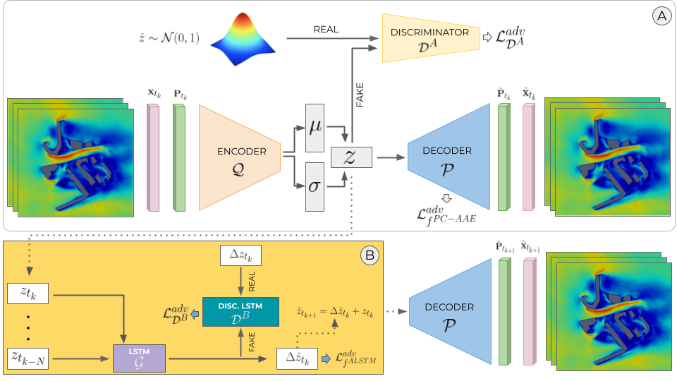
Figure 1: Workflow. Network A: PC-based adversarial autoencoder. Network B: Adversarial LSTM. Solid lines input within the same network, dashed lines input to another network.

2.1 Principal Components Analysis

As described by Lever et al. (2017), PCA is an unsupervised learning method that simplifies high-dimensional data by transforming it into fewer dimensions. Let $\mathbf{x}=\left\{\mathbf{x}_{t}\right\}_{t=1,\dots,n}$ with $\mathbf{x}\in\Re^{n\times m}$, with $n<m$, denotes the matrix of the model vectors at each time step. The PCA consists in decomposing this dataset as $\mathbf{x}=\mathbf{P}\mathbf{\Pi}+\mathbf{\bar{x}}$ where $\bf{P}\in\it{\mathbb{\Re}^{n\times n}}$ are the principal components of $\mathbf{x}$; $\bf{\Pi}\in\it{\mathbb{\Re}^{n\times m}}$ are the Empirical Orthogonal Functions; and $\mathbf{\bar{x}}$ is the mean vector of the model. The dimension reduction of the system comes from truncating $\mathbf{P}$ at the first $\tau$ PCs as $\mathbf{x}_{\tau}=\mathbf{P}_{\tau}\mathbf{\Pi}_{\tau}+\mathbf{\bar{x}}$, with $\mathbf{P}_{\tau}\in\Re^{n\times\tau}$ and $\mathbf{\Pi}_{\tau}\in\Re^{\tau\times m}$.

2.2 PC-based adversarial autoencoder

Once the PCs are obtained, they are utilised to train an adversarial autoencoder (AAE). The functional of our PC-based adversarial autoencoder (PC-AAE) is defined as:

$$f^{PC-AAE}:\mathbf{P}_{t_{k}}\to\tilde{\mathbf{P}}_{t_{k}}$$ (1)

where $\mathbf{P_{t_{k}}}$ are the scaled principal components time series between -1 and 1 at time-level $k$. The autoencoder consists of an encoder $\mathcal{Q}$ and a decoder $\mathcal{P}$, both mirrored fully-connected networks, where $\tilde{\mathbf{P}}_{t_{k}}=\mathcal{P}(\mathcal{Q}(\mathbf{P_{t_{k}}}))$.

Let $q(\mathbf{z}|\mathbf{P})$ and $p(\tilde{\mathbf{P}}|\mathbf{z})$ be the encoding and decoding distributions, respectively. As suggested by Makhzani et al. (2015), we use a Gaussian posterior and assume that $q(\mathbf{z}|\mathbf{P})$ is a Gaussian distribution, where its mean and variance are predicted by the encoder $\mathcal{P}$: $\mathbf{z}\sim\mathcal{N}(\mu(\mathbf{P}),\sigma(\mathbf{P}))$. This is achieved by adding two dense layers of means $\mu$ and $log\ \sigma$, (see Figure 1) to the final layer of the encoder $\mathcal{Q}$, and return $\mathbf{z}$ as a vector of samples. To ensure that $\mathbf{z}\sim q(\mathbf{z})=\mathcal{N}(\mu,\sigma^{2})$, the aggregated posterior, we use the reparameterisation trick described by Kingma & Welling (2013) for backpropagation through the network $\mathbf{z}=\mu+\sigma\odot\mathbf{\epsilon}$, where $\mathbf{\epsilon}$ is an auxiliary noise variable $\mathbf{\epsilon}\sim\mathcal{N}(0,\mathbf{I})$.

The adversarial training of PC-AAE includes a discriminator $\mathcal{D}^{A}$ to distinguish between the real samples, given by an arbitrary prior $p(\mathbf{z})\sim\mathcal{N}(0,\mathbf{I})$ and $q(\mathbf{z})$. Therefore, the adversarial autoencoder is regularised by matching $p(\mathbf{z})$ to $q(\mathbf{z})$. The $\mathbf{P}$ are fed to the discriminator as real sequences (ground truth). Let, $\mathcal{D}^{A}(\alpha,\beta)$ represent the discriminator function with an input $\alpha$ and a target label $\beta$ such that, for $\alpha=\hat{\mathbf{z}}\sim p(\mathbf{z})$, $\beta=1$ and for $\alpha=\mathbf{z}\sim q(\mathbf{z})$, $\beta=0$ . The training of $\mathcal{D}^{A}$ is based on the minimisation of the binary cross-entropy loss ($\mathcal{L}^{bce}$), using the Nesterov Adam optimizer (Nadam) (Dozat, 2016). The adversarial losses $\mathcal{L}^{adv}$ for $\mathcal{D}^{A}$ and $f^{PC-AAE}$ are then defined as:

$$\mathcal{L}^{adv}_{\mathcal{D}^{A}}(\mathbf{P}) =\mathcal{L}^{bce}_{\hat{\mathbf{z}}\sim p(\mathbf{z})}(\mathcal{D}^{A}(\hat{\mathbf{z}}),1))+\mathcal{L}^{bce}_{\mathbf{z}\sim q(\mathbf{z})}(\mathcal{D}^{A}(\mathbf{z}),0))$$ (2)

$$\mathcal{L}^{adv}_{f^{PC-AAE}}(\mathbf{P}) =\mathcal{L}^{bce}_{\mathbf{z}\sim q(\mathbf{z})}(\mathcal{D}^{A}(\mathbf{z}),1))+\mathcal{L}^{mse}(\tilde{\mathbf{P}},\mathbf{P})$$ (3)

where $\mathcal{L}^{mse}$ is the mean squared error (mse) between $\tilde{\mathbf{P}}$ and $\mathbf{P}$.

2.3 Adversarially long short-term memory network

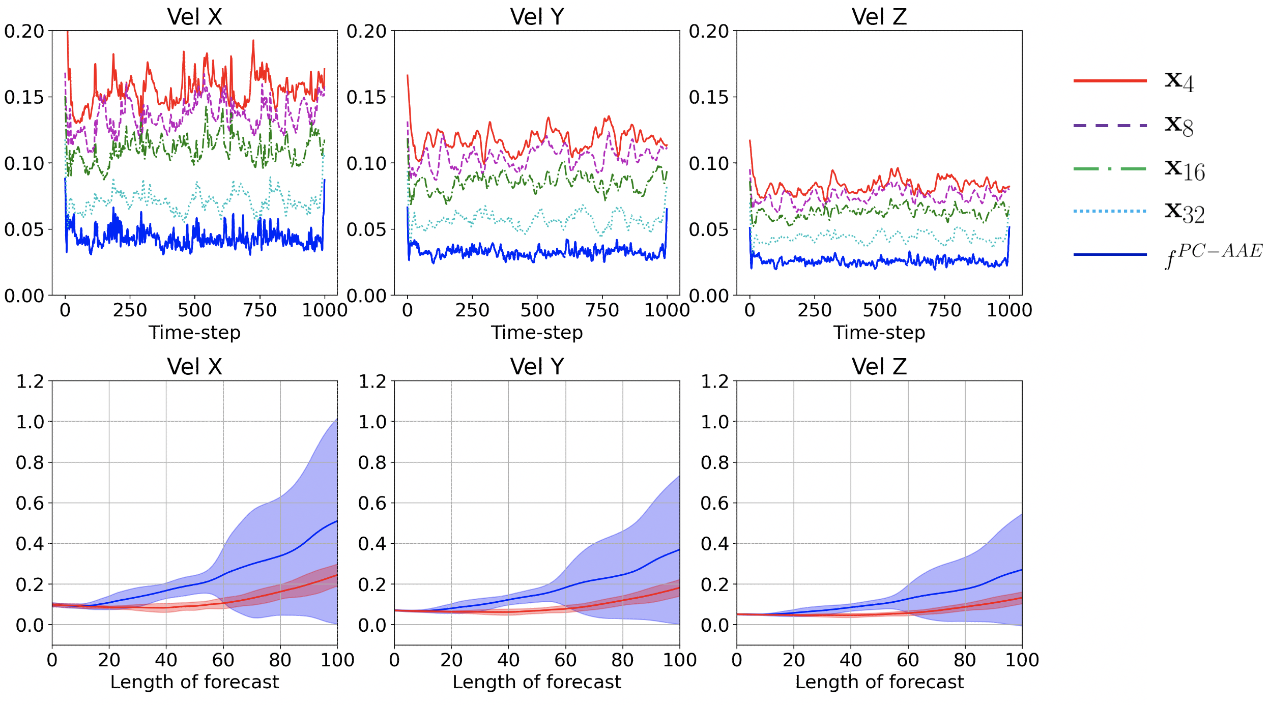
Figure 2: Mean absolute error in $ms^{-1}$. Top: $f^{PC-AAE}$ and reconstruction $\mathbf{x}_{\tau}$ with $\tau=\{4,8,16,32\}$ principal components. Bottom: Ensemble of forecast errors with $f^{Classic\,LSTM}$ (blue) and $f^{ALSTM}$ (red) from different starting points from $t=200$ to $t=250$ using 8 dimensions in the latent space. The solid line is the mean and the shaded area is one standard deviation.

Once the latent space $\mathbf{z}$ is obtained, it can be used to train a LSTM (Hochreiter & Schmidhuber, 1997) to make predictions. In this paper, an adversarial LSTM (ALSTM) network takes $N$ previous time-levels of $\mathbf{z}_{t_{k-N}},\dots,\mathbf{z}_{t_{k}}$ as input and predicts an approximation of $\mathbf{z}_{t_{k+1}}$ named $\tilde{\mathbf{z}}_{t_{k+1}}$. The functional of ALSTM is defined as:

$$f^{ALSTM}:\mathbf{z}_{t_{k-N}},\dots,\mathbf{z}_{t_{k}}\to\tilde{\mathbf{z}}_{t_{k+1}}$$ (4)

Our methodology proposes to add adversarial training to the LSTM network to further improve the forecasts. Similar to the adversarial autoencoder described in 2.2, the adversarial training of the LSTM network $\mathcal{G}$ includes a mirrored LSTM discriminator $\mathcal{D}^{B}$ (see Figure 1). The LSTM network $\mathcal{G}$ is designed to predict $\Delta\tilde{\mathbf{z}}_{t_{k+1}}=\mathcal{G}(\mathbf{z}_{t_{k-N}},\dots,\mathbf{z}_{t_{k}})$, with $\Delta\tilde{\mathbf{z}}_{t_{k}}=\tilde{\mathbf{z}}_{t_{k+1}}-\mathbf{z}_{t_{k}}$. Similar to $\mathcal{D}^{A}$, $\mathcal{D}^{B}$ takes $\Delta\mathbf{z}_{t_{k}}=\mathbf{z}_{t_{k+1}}-\mathbf{z}_{t_{k}}$ as a positive sample, and $\Delta\tilde{\mathbf{z}}_{t_{k}}$ as a negative sample. The training of $\mathcal{D}^{B}$ is based on the binary cross-entropy loss, with Nadam, as follows:

$$\mathcal{L}^{adv}_{\mathcal{D}^{B}}(\Delta\mathbf{z}) =\mathcal{L}^{bce}(\mathcal{D}^{B}(\Delta\mathbf{z},1))+\mathcal{L}^{bce}(\mathcal{D}^{B}(\Delta\tilde{\mathbf{z}},0))$$ (5)

$$\mathcal{L}^{adv}_{f^{ALSTM}}(\Delta\mathbf{z}) =\mathcal{L}^{bce}(\mathcal{D}^{B}(\Delta\tilde{\mathbf{z}},1))+\mathcal{L}^{mse}(\Delta\tilde{\mathbf{z}},\Delta\mathbf{z})$$ (6)

Thus, the prediction of the next time-level in the latent space $\tilde{\mathbf{z}}_{t_{k+1}}$ comes from $\tilde{\mathbf{z}}_{t_{k+1}}=\Delta\tilde{\mathbf{z}}_{t_{k}}+\mathbf{z}_{t_{k}}$. Once both networks are trained, the prediction of the next time-level in the physical space $\tilde{\mathbf{x}}_{t_{k+1}}$ is given by $\tilde{\mathbf{x}}_{t_{k+1}}=\mathcal{P}(\tilde{\mathbf{z}}_{t_{k+1}})+\bar{\mathbf{x}}$.

2.4 Domain

The computational fluid dynamics (CFD) simulations were carried out using Fluidity (Davies et al., 2011). The 3D case is a realistic case including 14 buildings representing a real urban area located near Elephant and Castle, South London, UK. The 3D case ($720m\times 676m\times 250m$) is composed of an unstructured mesh including $m=100,040$ nodes per dimension and $n=1000$ time-steps

A log-profile velocity (representing the wind profile of the atmospheric boundary layer) is used in the 3D case. The building facades and bottom surface have no-slip boundary conditions. Whilst, top and sides of the domain have a free-slip boundary condition. A more detailed description can be found in Arcucci et al. (2019).

3 Results and discussion

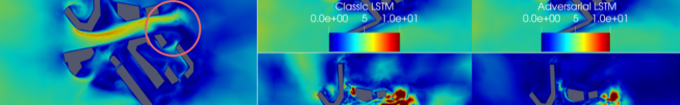
Figure 3: Comparison of forecasted velocity in $ms^{-1}$ (magnitude) fields by $f^{Classic\,LSTM}$ and $f^{ALSTM}$ and the absolute error with respect to the ground truth. This is a 80 time-step forecast starting from $t=200$. This is a horizontal slice normal to the Z-axis 10 m above ground.

A PCA was applied to a 3-dimensional velocity field $(ms^{-1})$. The full-rank PCs were used as input for the AAE and divided in 4 different experiments named $LS_{\tau}$ and compared to the corresponding reconstruction $\mathbf{x}_{\tau}$ with $\tau=\{4,8,16,32\}$ PCs. The results of the mean absolute error using the different dimension reduction approaches are shown in Figure 2. The AAE outperforms a simple truncation of the PCs. Additionally, the solution is robust and shows similar results regarding how many dimensions are chosen in the latent space of the bottleneck layer of the AAE. Therefore, the following forecast results are based on a dimension reduction using 8 dimensions in the latent space of the AAE, which is a compression of 5 orders of magnitude. The chosen architectures, hyperparameters and training options are shown in Appendix A.

Figure 2 presents the error from an ensemble of forecasts, of velocities in X, Y, Z, starting from different time-steps. The solid line represents the mean of the error ensemble and the shaded area is the standard deviation. The forecasts are created by using previous time-steps from data and producing a forecast which is subsequently used as an input for the prediction of the next time-step. The forecast experiments are named $F_{\tau}$. After 100 iterations, it is very clear that $f^{ALSTM}$ outperforms a LSTM with the same architecture without adversarial training, named $f^{Classic\,LSTM}$. The forecasts are 4 orders of magnitude faster than the CFD simulation.

Figure 3 shows the comparison of forecasted magnitude velocity (in $ms^{-1}$) fields of $f^{ALSTM}$, with 8 dimensions in the latent space, and $f^{Classic\,LSTM}$, with 8 PCs, from $t=200$. The snapshots clearly show that after 80 time-levels of forecasting, $f^{Classic\,LSTM}$ diverges quickly from the underlying model state, while $f^{ALSTM}$ preserve more underlying physics. Furthermore, $f^{ALSTM}$ is able to recreate eddies accurately learnt from the underlying physics model (red circle in Figure 3). This approach outperforms (Quilodrán Casas et al., 2020) in terms of data compression and (Quilodrán-Casas et al., 2021) in terms of forecast length.

4 Conclusions

This paper presented the advantages of using adversarial training to improve the forecast or a CFD simulation of urban air pollution. The PC-based adversarial autoencoder architecture is robust and its dimension-reduction outperforms a simple truncation of PCs. Furthermore, it is shown that applying adversarial training to a LSTM outperforms a LSTM trained in a classical way. This is very important when accurate near real-time predictions are needed and not enough data is available. It can be observed that adversarially trained LSTM does not diverge greatly from the data it has learned, given the constraint of the discriminator network. The replacement of the CFD solution by these models will speed up the forecast process towards a real-time solution. And, the application of adversarial training could potentially produce more physically realistic flows. Furthermore, this framework is data-agnostic and could be applied to different CFD models where enough data is available.

Appendix A Appendix

Table 1: Architectures of the different networks used in this study for the adversarial autoencoders and the adversarial LSTMs. The encoder $\mathcal{Q}$, the decoder $\mathcal{P}$ and the discriminator $\mathcal{D}^{A}$ are fully-connected layers. In the forecasts experiments Generator $\mathcal{G}$ and Discriminator $\mathcal{D}^{B}$ are LSTM networks.

Experiments AE	Enc $\mathcal{Q}$	Dec $\mathcal{P}$	Disc $\mathcal{D^{A}}$	Experiments ALSTM	Gen $\mathcal{G}$	Disc $\mathcal{D}^{B}$
$LS_{32}$	1000	32	32	$F_{32}$	32	32
	64	64	1		64	64
	32	1000			32	1
$LS_{16}$	1000	16	16	$F_{16}$	16	16
	64	32	1		64	64
	32	64			16	1
	16	1000
$LS_{8}$	1000	8	8	$F_{8}$	8	8
	64	16	1		64	64
	32	32			8	1
	16	64
	8	1000
$LS_{4}$	1000	4	4	$F_{4}$	4	4
	64	8	1		64	64
	32	16			4	1
	16	32
	8	64
	4	1000
Batch Normalisation in-between layers				Batch Normalisation before final layer
Leaky ReLU with a slope of 0.3				Dropout 0.5
				Time-lag $=5$
Optimizer: Adam with Nesterov momentum with Learning rate $=10^{-3},\beta_{1}=0.9,\beta_{2}=0.999$

References

- Arcucci et al. (2019) Rossella Arcucci, Laetitia Mottet, Christopher Pain, and Yi-Ke Guo. Optimal reduced space for variational data assimilation. Journal of Computational Physics, 379:51–69, 2019.
- Cheng et al. (2020) M Cheng, Fangxin Fang, Christopher C Pain, and IM Navon. Data-driven modelling of nonlinear spatio-temporal fluid flows using a deep convolutional generative adversarial network. Computer Methods in Applied Mechanics and Engineering, 365:113000, 2020.
- Davies et al. (2011) D Rhodri Davies, Cian R Wilson, and Stephan C Kramer. Fluidity: A fully unstructured anisotropic adaptive mesh computational modeling framework for geodynamics. Geochemistry, Geophysics, Geosystems, 12(6), 2011.
- Dong & Yang (2019) Hao-Wen Dong and Yi-Hsuan Yang. Towards a deeper understanding of adversarial losses. arXiv preprint arXiv:1901.08753, 2019.
- Dozat (2016) Timothy Dozat. Incorporating Nesterov momentum into adam. 2016.
- Goodfellow et al. (2014) Ian Goodfellow, Jean Pouget-Abadie, Mehdi Mirza, Bing Xu, David Warde-Farley, Sherjil Ozair, Aaron Courville, and Yoshua Bengio. Generative adversarial nets. In Advances in neural information processing systems, pp. 2672–2680, 2014.
- Hochreiter & Schmidhuber (1997) Sepp Hochreiter and Jürgen Schmidhuber. Long short-term memory. Neural computation, 9(8):1735–1780, 1997.
- Kingma & Welling (2013) Diederik P Kingma and Max Welling. Auto-encoding variational bayes. arXiv preprint arXiv:1312.6114, 2013.
- Lever et al. (2017) Jake Lever, Martin Krzywinski, and Naomi Altman. Points of significance: Principal component analysis, 2017.
- Makhzani et al. (2015) Alireza Makhzani, Jonathon Shlens, Navdeep Jaitly, Ian Goodfellow, and Brendan Frey. Adversarial autoencoders. arXiv preprint arXiv:1511.05644, 2015.
- Meng & Chen (2017) Dongyu Meng and Hao Chen. Magnet: a two-pronged defense against adversarial examples. In Proceedings of the 2017 ACM SIGSAC conference on computer and communications security, pp. 135–147, 2017.
- Phillips et al. (2020) Toby Phillips, Claire E Heaney, Paul N Smith, and Christopher C Pain. An autoencoder-based reduced-order model for eigenvalue problems with application to neutron diffusion. arXiv preprint arXiv:2008.10532, 2020.
- Quilodrán Casas et al. (2020) César Quilodrán Casas, Rossella Arcucci, and Yike Guo. Urban air pollution forecasts generated from latent space representation. In ICLR 2020 Workshop on Integration of Deep Neural Models and Differential Equations, 2020.
- Quilodrán Casas et al. (2020) César Quilodrán Casas, Rossella Arcucci, Pin Wu, Christopher Pain, and Yi-Ke Guo. A Reduced Order Deep Data Assimilation model. Physica D: Nonlinear Phenomena, 412:132615, 2020.
- Quilodrán-Casas et al. (2021) César Quilodrán-Casas, Rossella Arcucci, Christopher Pain, and Yike Guo. Adversarially trained LSTMs on reduced order models of urban air pollution simulations. arXiv preprint arXiv:2101.01568, 2021.
- Quilodrán Casas (2018) César Quilodrán Casas. Fast ocean data assimilation and forecasting using a neural-network reduced-space regional ocean model of the north Brazil current. PhD thesis, Imperial College London, 2018.
- Reddy et al. (2019) Sandeep B Reddy, Allan Ross Magee, Rajeev K Jaiman, J Liu, W Xu, A Choudhary, and AA Hussain. Reduced order model for unsteady fluid flows via recurrent neural networks. In International Conference on Offshore Mechanics and Arctic Engineering, volume 58776, pp. V002T08A007. American Society of Mechanical Engineers, 2019.
- Shafahi et al. (2019) Ali Shafahi, Mahyar Najibi, Mohammad Amin Ghiasi, Zheng Xu, John Dickerson, Christoph Studer, Larry S Davis, Gavin Taylor, and Tom Goldstein. Adversarial training for free! In Advances in Neural Information Processing Systems, pp. 3358–3369, 2019.
- Wang et al. (2019) Dilin Wang, Chengyue Gong, and Qiang Liu. Improving neural language modeling via adversarial training. arXiv preprint arXiv:1906.03805, 2019.
- Xie et al. (2018) You Xie, Erik Franz, Mengyu Chu, and Nils Thuerey. Tempogan: A temporally coherent, volumetric gan for super-resolution fluid flow. ACM Transactions on Graphics (TOG), 37(4):1–15, 2018.