Count Network Autoregression
Abstract
We consider network autoregressive models for count data with a non-random neighborhood structure. The main methodological contribution is the development of conditions that guarantee stability and valid statistical inference for such models. We consider both cases of fixed and increasing network dimension and we show that quasi-likelihood inference provides consistent and asymptotically normally distributed estimators. The work is complemented by simulation results and a data example.
Keywords: generalized linear models, increasing dimension, link function, multivariate count time series, quasi-likelihood.
AMS 2020 subject classification: 62M10
1 Introduction
The vast availability of integer-valued data, emerging from several real world applications, has motivated the growth of a large body of literature for modeling and inference of count time series processes. For comprehensive surveys, see Kedem and Fokianos (2002), Weiß (2018) Davis et al. (2021), among others. The aim of this contribution is to develop a statistical framework for network count time series which are simply multivariate time series equipped with a neighborhood structure. Consider the vector which consists of all node measurements at some time . This is going to be the response vector we will be studying and we will assume that its evolution is influenced not only by past observations but also by its neighbors. We consider such processes assuming that their neighborhood structure is known. We deal with a multivariate problem whose main challenge is that the response vector is high-dimensional and therefore we study, in detail, this case as we explain below.
1.1 Related Work
Early contributions to the development of count time series models were the Integer Autoregressive models (INAR) Al-Osh and Alzaid (1987); Alzaid and Al-Osh (1990) and observation (Zeger and Liang, 1986) or parameter driven models (Zeger, 1988). The latter classification, due to Cox (1981), will be particularly useful as we will be developing theory for count observation-driven models.
In this contribution, we appeal to the generalized linear model (GLM) framework, see McCullagh and Nelder (1989), as it provides a natural extension of continuous-valued time series to integer-valued processes. The GLM framework accommodates likelihood inference and supplies a toolbox whereby testing and diagnostics can also be advanced. Some examples of observation-driven models for count time series include the works by Davis et al. (2003), Heinen (2003), Fokianos and Kedem (2004) and Ferland et al. (2006), among others. Related work includes Fokianos et al. (2009) and Fokianos and Tjøstheim (2011) who develop properties and estimation for a class of linear and log-linear count time series models. Further related contributions have appeared over the last years; see Christou and Fokianos (2014) for quasi-likelihood inference of negative binomial processes, Ahmad and Francq (2016) for quasi-likelihood inference based on suitable moment assumptions. In addition, Douc et al. (2013), Dunsmuir (2016), Davis and Liu (2016), Cui and Zheng (2017), Douc et al. (2017) and more recently Armillotta et al. (2022), among others, provide further generalizations of observation-driven models leaning on general distribution functions or one-parameter exponential family of distributions. Theoretical properties of such models have been fully investigated using various techniques; Fokianos et al. (2009) developed initially a perturbation approach, Neumann (2011) employed the notion of -mixing, Doukhan et al. (2012) (weak dependence approach), Woodard et al. (2011) and Douc et al. (2013) (Markov chain theory without irreducibility assumptions) and Wang et al. (2014) (using -chains theory; see Meyn and Tweedie (1993)).
Studies of multivariate INAR models include those of Latour (1997), Pedeli and Karlis (2011, 2013a, 2013b), among others. Theory and inference for multivariate count time series models is a research topic which is receiving increasing attention. In particular, observation-driven models and their properties are discussed by Heinen and Rengifo (2007), Liu (2012), Andreassen (2013), Ahmad (2016) and Lee et al. (2018). More recently, Fokianos et al. (2020) introduced a multivariate extension of the linear and log-linear Poisson autoregression model, by employing a copula-based construction for the joint distribution of the counts. The authors employ Poisson processes’ properties to introduce joint dependence of counts over time. In doing so, they avoid technical difficulties associated with the non-uniqueness of copula for discrete distributions (Genest and Nešlehová, 2007, pp. 507-508). They propose a plausible data generating process which preserves, marginally, Poisson processes’ properties, conditional on the past. Further details are given by the recent review of Fokianos (2022).
1.2 Network Time Series
Multivariate observation-driven count time series models are useful for modeling time-varying network data. Such data is increasingly available in many scientific areas (social networks, epidemics, etc.). Measuring the impact of a network structure to a multivariate time series process has attracted considerable attention over the last years. In an unpublished work, Knight et al. (2016) defined multivariate continuous time series coupled with a network structure as network time series. Furthermore these authors proposed methodology for the analysis of such data. Such approach has been originally proposed in the context of spatio-temporal data analysis, referred to as Space-Time Autoregressive Moving Average (STARMA) models; Cliff and Ord (1975), Martin and Oeppen (1975) and Pfeifer and Deutrch (1980), among many others. In general, any stream of data for a sample of units whose relations can be modeled through an adjacency matrix (neighborhood structure), adhere to statistical techniques developed in this work. Zhu et al. (2017) have discussed a similar model, called Network Autoregressive model (NAR), which is an autoregressive model for continuous valued network data and established associated least squares inference under two asymptotic regimes (a) with increasing time sample size and fixed network dimension and (b) with both increasing. More precisely, it is assumed that and , i.e. the temporal sample size is assumed to depend on . The regime (a) corresponds to standard asymptotic inference in time series analysis. However, in network analysis it is important to understand the behavior of the process when the network’s dimension grows. This is a relevant problem in fields where typically the network is large, see, for example, social networks in Wasserman et al. (1994). It is also essential to have stability conditions for large network structures, so that proper time series inference can be advanced; those problems motivate study of asymptotics under regime (b). Significant extension of this work to network quantile autoregressive models has been recently reported by Zhu et al. (2019). Some other extensions of the NAR model include the grouped least squares estimation (Zhu and Pan, 2020) and a network version of the GARCH model, see Zhou et al. (2020) but for the case of and fixed network dimension . Under the standard asymptotic regime (a), related work was also developed by Knight et al. (2020) who specified a Generalized Network Autoregressive model (GNAR) for continuous random variables, which takes into account different layers of relationships within neighbors of the network. Moreover, the same authors provide R software (package GNAR) for fitting such models.
1.3 Our contribution
Integer-valued responses are commonly encountered in real applications and are strongly connected to network data. For example, several data of interest in social network analysis correspond to integer-valued responses (number of posts, number of likes, counts of digit employed in comments, etc). Another typical field of application is related to the number of cases in epidemic models for studying the spread of infection diseases in a population; this is even more important in the current COVID-19 pandemic outbreak. Recently, an application of this type which employs a model similar to the NAR with count data has been suggested by Bracher and Held (2020). Therefore, the extension of the NAR model to multivariate count time series is an important theoretical and methodological contribution which is not covered by the existing literature, to the best of our knowledge.
The main goal of this work is to fill this gap by specifying linear and log-linear Poisson network autoregressions (PNAR) for count processes and by studying in detail the two related types of asymptotic inference discussed above. Moreover, the development of all network time series models discussed so far relies strongly on the assumption that the innovations are Independent and Identically Distributed (IID). Such a condition might not be realistic in many applications. We overcome this limitation by employing the notion of -near epoch dependence (NED), see Andrews (1988), Pötscher and Prucha (1997), and the related concept of -mixing (Rosenblatt, 1956; Doukhan, 1994). These notions allow relaxation of the independence assumption as they provide some guarantee of asymptotic independence over time. An elaborate and flexible dependence structure among variables, over time and over the nodes composing the network, is available for all models we consider due to the definition of a full covariance matrix, where the dependence among variables is captured by the copula construction introduced in Fokianos et al. (2020). For an alternative approach to modeling multivariate counts in continuous time see Veraart (2019), Eyjolfsson and Tjøstheim (2023), and Fang et al. (2021) for a network model employing Hawkes processes which are related to the linear and log-linear model we will be studying. Indeed those models are obtained after suitable discretization of the corresponding continuous time process. However our proposal imposes a specific data generating process, does not assume homogeneity across the network and the condition required for obtaining good large sample properties of the QMLE are quite different than those assumed by Fang et al. (2021).
For the continuous-valued case, Zhu et al. (2017) employed ordinary least square (OLS) estimation combined with specific properties imposed on the adjacency matrix for the estimation of unknown model parameters. However, this method is not applicable to general time series models. In the case we study, estimation is carried out by using quasi-likelihood methods; see Heyde (1997), for example. When the network dimension is fixed and , standard results for Quasi Maximum Likelihood Estimation (QMLE) from multivariate count autoregressions, as developed by Fokianos et al. (2020), carry over to the case of PNAR models. When the network dimension is increasing, the asymptotic properties of the estimators would rely on the ergodicity of a stationary random process with . However, there exists no widely accepted definition for stationarity of a process with infinite dimension. Consequently no ergodicity results are available for processes with and standard time series results concerning convergence of sample means do not carry over to the increasing dimension case. In the present contribution, this problem is bypassed by providing an alternative proof, based on the laws of large numbers for -NED processes of Andrews (1988). Our method employs the working definition of stationarity of Zhu et al. (2017, Def. 1) for processes of increasing dimension. All these developments are crucial to a thorough study of QMLE under the double regime asymptotics we consider. Finally, we are addressing several other related problem, including estimation of contemporaneous dependence and improving the efficiency of the QMLE.
1.4 Outline
The paper is organized as follows: Section 2 discusses the PNAR() model specification for the linear and the log-linear case, with lag order , and the related stability properties. In Section 3, quasi-likelihood inference is established, showing consistency and asymptotic normality of the QMLE for the two types of asymptotics (a)-(b). Section 4 discusses the results of a simulation study and an application on real data. The paper concludes with an Appendix containing the proofs of Theorem 1 and Lemma 1-2. All the other proofs are included in the Supplementary Material (abbreviated by SM) together with additional results.
Notation:
We denote the -norm of a -dimensional vector . If , . Let the -norm for a random vector . For a matrix , , denotes the generalized matrix norm . If , then . If , , where is the spectral radius. If , . If , then these norms are matrix norms. Define the largest absolute eigenvalue of a symmetric matrix . Define , and the elementwise -norm for vectors, matrices and random vectors, respectively. Moreover, denote by a partial order relation on such that means for . For a -dimensional vector , with , set the following compact notation . The notations and denote a constant which depend on , where . In particular denotes a generic constant. Finally, throughout the paper the notation will be used as a shorthand for and , where the temporal size is assumed to depend on the network dimension .
2 Stability results for count network time series
We consider a network with nodes (network size) and index . The structure of the network is completely described by the adjacency matrix , i.e. provided that there exists a directed edge from to , (e.g. user follows on Twitter), and otherwise. However, undirected graphs are allowed (). The structure of the network is assumed non-random, by this we mean that the network is known with fixed edges; see also Zhu et al. (2017). Self-relationships are not allowed, i.e. for any ; this is a typical assumption, and it is reasonable for various real situations, e.g. social networks, where users do not follow themselves; see Wasserman et al. (1994), Kolaczyk and Csárdi (2014). Define a count variable for the node at time . We want to assess the effect of the network structure on the count variable for over time .
In this section, we study the properties of linear and log-linear models. We initiate this study by considering a simple, yet illuminating, case of a linear model of order one and then we consider the more general case of ’th order model. Finally, we discuss log-linear models. In what follows, we denote by an -dimensional vector of count time series with be the corresponding -dimensional intensity process vector. Define by . Based on the specification of the model, we assume that .
2.1 Linear PNAR(1) model
A linear count network model of order 1, is given by
| (1) |
where and is the out-degree, i.e the total number of nodes which has an edge with. From the left hand side equation of (1), we observe that the process is assumed to be marginally Poisson, conditionally to the past. We call (1) linear Poisson network autoregression of order 1, abbreviated by PNAR(1).
Model (1) postulates that, for every single node , the marginal conditional mean of the process is regressed on the past count of the variable itself for and the average count of the other nodes which have a connection with . This model assumes that only the nodes which are directly followed by the focal node possibly have an impact on the mean process of counts. It is a reasonable assumption in many applications. For example, in a social network, the activity of node , which satisfies , does not affect node . The parameter is called network effect, as it measures the average impact of node ’s connections . The coefficient is called momentum effect because it provides a weight for the impact of past count . This interpretation is in line with the Gaussian NAR as discussed by Zhu et al. (2017) for the case of continuous variables.
Equation (1) does not include information about the joint dependence structure of the PNAR(1) model. Then the goal is to introduce a multivariate random vector, at each time point , whose each component follow marginally the Poisson distribution (conditionally to the past) but there exists among them arbitrary correlation. In a recent work, Fokianos et al. (2020) defined such a distribution in terms of a data generating process specified by an algorithm which generates a random vector whose dependence among their components is introduced by imposing a copula on the waiting times of a Poisson process; see also (Fokianos, 2022, p.4). In this way, we can, define the multivariate copula Poisson distribution with parameter, say , and denote it by , as an -dimensional random vector whose components are marginally Poisson distributed with mean , and whose structure of dependence is modeled through the copula on their associated exponential waiting times random variables. It is then convenient to rewrite (1) in vectorial form, following Fokianos et al. (2020),
| (2) |
where , with , and the matrix , where is the row-normalized adjacency matrix, with , so is the -th row vector of the matrix , satisfying , and is the identity matrix. In general, the weights can be chosen arbitrarily as long as is satisfied. To obtain insight for the data generating process, as introduced by (2), consider a set of values and a starting vector ,
-
1.
Let , for a sample from a -dimensional copula , where follows a Uniform(0,1) distribution, for .
-
2.
The transformation follows the exponential distribution with parameter , for .
-
3.
If , then , otherwise , by taking large enough. Then, , for . So, is a set of (conditionally) marginal Poisson processes with mean .
-
4.
By using the model (2), is obtained.
-
5.
Return back to step 1 to obtain , and so on.
In practical applications the sample size should be a large value, e.g. ; its value clearly depends, in general, on the magnitude of observed data. Moreover, the copula construction will depend on one or more unknown parameters, say , which capture the contemporaneous correlation among the variables.
The previous algorithm generates a sample of multivariate counts for practical simulations. In principle, the algorithm simulates realizations of a stochastic process , i.e. for all integers. Accordingly, is not a fixed vector but , being a function of , then is equivalent to say . The same happens for ad so on. Then, the data generating process (DGP) generates being conditionally marginally Poisson for all .
The development of a multivariate count time series model would be based on specification of a joint distribution, so that the standard likelihood inference and testing procedures can be developed. Although several alternatives have been proposed in the literature, see the review in Fokianos (2022, Sec. 2), the choice of a suitable multivariate version of the conditional Poisson probability mass function (p.m.f) is a challenging problem. In fact, multivariate Poisson-type p.m.f have usually complicated closed form and the associated likelihood inference is theoretically and computationally cumbersome. Furthermore, in many cases, the available multivariate Poisson-type p.m.f. implicitly imply restrictions on models with limited use in applications (e.g. covariances always positive, constant pairwise correlations). In this work the joint distribution of the vector is constructed by following the copula approach described above. The proposed DGP ensures that all marginal distributions of are univariate Poisson, conditionally to the past, as described in (1), while it introduces an arbitrary dependence among them in a flexible and general way by the copula construction. See Inouye et al. (2017) and Fokianos (2022) for a discussion on the choice of multivariate count distributions and several alternatives. Further results regarding the empirical properties of model (2) are discussed in Section S-1.2 of SM.
We choose the conditional multivariate copula Poisson distribution for its simplicity and because it is a natural distributional assumption for counting number of events over a time period. However, any multivariate count distribution whose mean is modeled through (1) and possesses moments up to an appropriate order fits the QMLE methodology which employs (10) to derive consistent and asymptotically normally distributed estimators. In fact, theory and applications can be extended to other count distributions. By exploiting the same copula construction and modifying suitably the generation of exponential waiting times, we can define a conditional copula multivariate Negative Binomial distribution, and more generally a conditional copula mixed Poisson distribution; see Fokianos et al. (2020, p. 474). A complete treatment of such extensions remains unexplored.
2.2 Linear PNAR() model
More generally, we introduce and study an extension of model (1) by allowing to depend on the last lagged values. We call this the linear Poisson NAR() model and its defined analogously to (1) but with
| (3) |
where for all . If , set , to obtain (1). The joint conditional distribution of the vector is defined by means of the copula construction discussed in Sec. 2.1. Without loss of generality, we can set coefficients equal to zero if the parameter order is different in both terms of (3). Then (3) is rewritten as
| (4) |
where for by recalling that . The following result establishes sharp verifiable conditions for proving ergodicity, when is fixed.
Proposition 1.
Consider model (4), with fixed . Suppose that . Then, the process is stationary and ergodic with for any .
The result follows from Debaly and Truquet (2021, Thm. 2). Similar results have been recently proved by Fokianos et al. (2020) when the lagged conditional mean is added as a feedback term in the model. Following these authors, we obtain the same results of Proposition 1 but under stronger conditions. For example, when , we will need to assume either or to obtain identical conclusions. Results about the first and second order properties of model (3) are given in SM S-1; see also Fokianos et al. (2020, Prop. 3.2).
Proposition 1 establishes the existence of the moments of the count process with fixed , but this property is not guaranteed to hold when . The following results show that, is , the conclusions of Proposition 1 are still true.
Proposition 2.
Consider model (4) and . Then, , for any .
In order to investigate the stability results of the process when the network size is diverging () we employ the working definition of stationarity for increasing dimensional processes as discussed by Zhu et al. (2017, Def. 1). The following result holds.
Theorem 1.
Consider model (4). Assume and . Then, there exists a unique strictly stationary solution to the linear PNAR() model, with , for all .
Theorem. 1 extends (Zhu et al., 2017, Thm.1). Although stronger than the conditions of Proposition 1, allows to prove stationarity for increasing network size and the existence of moments of the process; moreover, it is more natural assumption than the condition , and it complements the existing work for continuous valued models; Zhu et al. (2017). It is worth pointing out that the copula construction is not used in the proof of Theorem 1 (see also Theorem 2 for log-linear model). However, it is used in Section 4.1 where we report a simulation study. It is interesting though, that even under this setup, stability conditions are independent of the correlation structure of innovations; this is similar to the case of multivariate ARMA models.
Remark 1.
Models (4) implies that are marginally Poisson distributed conditionally on the past of the process, . There is no any assumption about the marginal and joint unconditional distributions of the process. In general, the unconditional distribution of is unknown. However, from the results of Theorem 1 we can conclude that is a stationary Markov chain of order so its (unconditional) distribution exists, is unique, does not depend on and all its moments are uniformly bounded. Moreover, we derive explicitly the first two moments of such distribution (SM S-1).
Remark 2.
A count GNAR() extension similar to the model introduced by Knight et al. (2020, eq. 1), for the standard asymptotic regime (), in the context of continuous-valued random variables, is included in the framework we consider. Such model adds an average neighbor impact for several stages of connections between the nodes of a given network. That is, , for and , with the set of neighbors of the node . (So, for example, describes the neighbors of the neighbors of the node , and so on.) In this case, the row-normalized adjacency matrix have elements , where , denotes the cardinality of a set and is the indicator function. Several types of edges are allowed in the network. The Poisson GNAR() has the following formulation.
| (5) |
where is the maximum stage of neighbor dependence for the time lag and all the parameters of the model need to be non-negative. Model (5) can be included in the formulation (4) by setting . Since it holds that , we have . Hence, the result of the present contribution, i.e. existence of the moments of the model, the related stability properties and the associated inferential results, under the standard asymptotic regime, apply to (5).
2.3 Log-linear PNAR models
Recall model (1). The network effect of model (1) is typically expected to be positive, see Chen et al. (2013), and the impact of is positive, as well. Hence, positive constraints on the parameters are theoretically justifiable as well as practically sound. However, in order to allow a natural link to the GLM theory, McCullagh and Nelder (1989), and allowing the possibility to iclude covariates as well as real valued coefficients, we additionally study the following log-linear model, see Fokianos and Tjøstheim (2011):
| (6) |
where for every . No parameters constraints are required for model (6) since . Interpretation of all parameters is the same, as in the case of (1), but in the logarithmic scale. Again, the model can be rewritten in vectorial form, as in the case of model (2)
| (7) |
where is an -dimensional copula conditional Poisson distribution, as above. Furthermore, it can be useful rewriting the model as follow.
where . By Lemma A.1 in Fokianos and Tjøstheim (2011) as , so is approximately martingale difference sequence (MDS). This means that the formulation of first two moments established for the linear model in SM S-1 hold, approximately, for . We discuss empirical properties of the count process of model (6) in Section S-2.3 of the SM. Moreover, is a MDS. We define the log-linear PNAR() by
| (8) |
using the same notation as before. Then
| (9) |
where for . The following results are complementing Proposition 1-2 and Theorem 1 proved for the case of log-linear model.
Proposition 3.
Consider model (9), with fixed . Suppose that . Then the process is stationary and ergodic with . Moreover, if , there exists some such that and .
The result follows from Debaly and Truquet (2019, Thm. 5). Analogously to the linear model, we need to show the uniform boundedness of moments of the process and the stationarity of the model with increasing dimension. Since the noise is approximately MDS, the following result is proved by employing approximate arguments.
Proposition 4.
Consider model (9) and . Then, , and , for any .
Analogously to Theorem 1, a strict stationarity result for network of increasing order is given for the log-linear PNAR model (9).
Theorem 2.
Consider model (9). Assume and . Then, there exists a unique strictly stationary solution to the log-linear PNAR model, with , and , for all .
Remark 3.
For simplicity, model (4) has been defined without including covariates. But time-invariant positive covariates can be included without affecting the results of the present contribution, under suitable moments existence assumptions. This is a useful fact because we can consider available node-specific characteristics, for example. Moreover, the log-linear version (9) ensures the inclusion of covariates whose values belong to .
3 Quasi-likelihood inference for increasing network size
We develop inference for the unknown vector of parameters of models (4),(9), denoted by , where and is the parameter space. Full parametric likelihood inference requires specification of the conditional joint p.m.f., which is hard to obtain, because the exponential waiting times employed for steps 2-3 of the DGP algorithm are latent random variables. This implies that the imposed copula function cannot be used to obtain the full model likelihood. Nevertheless, the marginal conditional distributions of the DGP are well defined quantities and can be employed for estimation of unknown parameters. Then, the estimation problem is approached by using the quasi maximum likelihood theory; see Wedderburn (1974) and Gourieroux et al. (1984) among others. Developing proofs of consistency and asymptotic normality of the Quasi Maximum Likelihood Estimation (QMLE), when and , is the main goal of the present section. Define the conditional quasi log-likelihood function for the vector of unknown parameters by
| (10) |
which is the log-likelihood one would obtain if time series modeled in (4), or (9), are contemporaneously independent. Clearly such an approach does not require any specification/estimation of the copula structure and its set of parameters . Note that although the copula is not included in the maximization of the “working” log-likelihood (10), the QMLE is not computed under the assumption of independence; this is easily seen by the form of the information matrix (15) below, which depends on the true conditional covariance matrix of the process .
The quasi log-likelihood (10) allows computational simplifications and guarantees valid asymptotic properties of the estimator at the cost of a lower efficiency when compared top the full maximum likelihood estimator. In particular, (10) is a member of the one-parameter exponential family; then, even though we do not employ the true likelihood, Gourieroux et al. (1984, Thm. 1-3) gives an indication that the resulting estimator will be consistent and asymptotically normal. Note that we study a different framework since both are assumed to tend to infinity. Since is a non-random sequence of matrices indexed by , the specification of the asymptotic properties of the estimator deals with two diverging indexes, and , allowing to establish a double-dimensional-type of converge, when both the temporal size and the network dimension grow together. Assuming that there exists a true vector of parameter, say , such that the mean model specification (4) (or equivalently (9)) is correct, regardless the true DGP, then we obtain a consistent and asymptotically normal estimator by maximizing the quasi log-likelihood (10). This is a novel result as most contributions in the literature deal either with the case or fixed; see previous references.
Consider the linear PNAR model (4). Denote by , the QMLE for . The score function for the linear model is given by
| (11) | |||||
where
is a matrix and is the diagonal matrix with diagonal elements equal to for . The Hessian matrix (multiplied by -1) is given by
| (12) |
with and the conditional information matrix is
| (13) |
where denotes the true conditional covariance matrix of the vector and recalling . Expectation is taken with respect to the stationary distribution of . Moreover, the theoretical counterpart of the Hessian and information matrices, respectively, are the following.
| (14) |
| (15) |
Similarly for the log-linear PNAR model, we have that the score function is given by:
| (16) |
where
is a matrix, and
| (17) |
where is the diagonal matrix with diagonal elements equal to for and with . Moreover,
| (18) |
| (19) |
are respectively (minus) the Hessian matrix and the information matrix.
3.1 Linear model inference
Recall (10). We drop the dependence on when a quantity is evaluated at . For ease of presentation, consider model (2) with first moment where (see SM S-1). Moreover, the elementwise absolute value of the error covariance matrix is defined as . Define the following expectations , , , . Those expectations constitute summands for some of the elements of the expected third derivative matrix of . Consider the set , is the set of indices where the absolute value of the third derivative is maximum. Assume the following:
-
B1
The process is -mixing, where .
-
B2
Let be a sequence of matrices with non-random entries indexed by .
-
B2.1
Consider as a transition probability matrix of a Markov chain, whose state space is defined as the set of all the nodes in the network (i.e., ). The Markov chain is assumed to be irreducible and aperiodic. Further, define as the stationary distribution of the Markov chain, where , and . Furthermore, assume that as .
-
B2.2
Define and assume that and , for some .
-
B2.1
-
B3
Set , and . Assume the following limits exist: , , , and, if , .
Assumption B1 (see Doukhan (1994)) is a mixing condition. Recall that is an -mixing array if, namely,
where , . This assumption holds true for the simple example of where is constructed by the copula method proposed in this paper. In this case, the noise is independent over time but it is non contemporaneous independent. Another example would be all the processes which satisfy , where is some function which does not depend on , such that as .
Assumption B2 on the network structure implies that the edges between nodes are known and as increases to an additional node is added with some edges to the previous nodes, but the edges among the previous nodes do not change. Moreover, it requires some uniformity conditions, and it is equivalent set of conditions as Zhu et al. (2019, C2, C2.1-C2.2). Finally, B2.2 requires that the network structure admits certain uniformity property ( diverges slowly). Zhu et al. (2017, Supp. Mat., Sec. 7.1-7.3) found empirically that this is the case for several network models. In our case, regularity assumptions on the structure of dependence among the errors, when the network grows, are required by imposing that the diverging rate of will be slower than order , in B2.2, and its product with the squared sum of the stationary distribution of the chain, , will tend to 0, in B2.1. We give an empirical verification of such conditions in Section S-4 of the SM. In the continuous-valued case introduced in Zhu et al. (2017) such assumptions are not necessary because the errors are IID with common variance . Moreover, in this case, the absolute value is no more required because .
The conditions outlined in B3 are law of large numbers-like assumptions, which are quite standard in the existing literature, since little is known about the behavior of the process as . These assumptions are required to guarantee that the Hessian matrix (12) converges to a matrix which exists. Section S-4 includes numerical study examples showing the validity of these limits. If OLS estimation with IID errors was performed, conditions B3 would correspond exactly to those in Zhu et al. (2017, C3).
Lemma 1.
Some preliminary results required to show the lemma are proved in SM S-3.1. The proof of Lemma 20 is given in Appendix A.2.
Consider now the following conditions:
-
B3′
Set , , and . Assume that the following limits exist:
, , ,
and, if , . -
B4
There exists a non negative, non increasing sequence such that and, for , almost surely
(21)
Condition B3′ is simply an extension of assumption B3, required for the convergence of the conditional information matrix (13) to a valid limiting information matrix, see below. More precisely, the reader can verify that B3 is just a special case of B3′, when . The main reason that this assumption is introduced is that, for the QMLE, the conditional information matrix and the Hessian matrix are, in general, different. This does not occur in the case studied by Zhu et al. (2017). Analogously to B3, when is continuous-valued random vector, and we deal with IID errors , B3′ reduces again to the conditions in Zhu et al. (2017, C3).
Assumption B4 could be considered as a contemporaneous weak dependence condition. Indeed, even in the very simple case of independence model, i.e. , for all , the reader can easily verify that, without any further constraints, , so the limiting variance of the estimator will eventually diverge, since it depends on the limit of the conditional information matrix. Instead, under B4, , and the existence of the limiting covariance matrix can be shown, as in Lemma 22 and Theorem 3 below. Insights about weak dependence conditions have been stated in Zhu et al. (2017, p. 1102). When the errors are independent over different nodes and the past (Zhu et al., 2017, C1), B4 is trivially satisfied, since , for . See Section S-5 of the SM, for an example where B4 is empirically verified. Define , a non-null real-valued vector.
Lemma 2.
Note that the assumption is not implied by condition B4 which is satisfied provided that (21) holds true for higher-order moments of the vectors ; See Section S-6 more.
Theorem 3.
Consider model (2). Let . Suppose that is compact and assume that the true value belongs to the interior of . Suppose that the conditions of Lemma 20-22 hold. Then, there exists a fixed open neighborhood of such that with probability tending to 1 as , for the score function (11), the equation has a unique solution, called , which is consistent and asymptotically normal:
The extension of Theorem 3 to the general order linear PNAR() model is immediate, by using the well-know VAR(1) companion matrix; see (S-1). Assumptions B1-B2 and B4 remain substantially unaffected, using Debaly and Truquet (2021, Lemma 1.1). B3-B3′ can be suitably rearranged similarly to Zhu et al. (2017, C4) and the result follows by Zhu et al. (2017, Supp. Mat., Sec. 4). We omit the details.
Remark 5.
A standard asymptotic inference result, with , is obtained for the QMLE , where the “sandwich‘” covariance is , by Theorem 3, as a special case, when is fixed. This result requires only the stationarity conditions of Proposition 1, the compactness of the parameter space, and assuming that the true value of the parameters belongs to its interior. Such result is proved along the lines of Theorem 4.1 in Fokianos et al. (2020). Similar comments apply also for the log-linear model below. The case, where fixed and diverging, cannot be studied in the framework we consider, since the convergence of the quantities involved in Lemmas 20-22 requires both indexes to diverge together. For details see also the related proofs in the Appendix A.2. This is empirically confirmed by some numerical bias found in the simulations of Sec. 4.1, when is small compared to .
Remark 6.
It is worth pointing out that model (2) may be extended by including a feedback process such as as
| (23) |
where and will be a network and autoregressive coefficients, respectively, for the past values of the conditional mean process. Such extension is suitable when the mean process depends on the whole past history of the count process. When the network dimension is fixed, model (23) is just a special case of Fokianos et al. (2020, eq. 3), with a specific neighbor structure of the coefficients matrices therein. The stability conditions and asymptotic properties of the QMLE follow immediately. Note that (23) implies , so all likelihood based quantities are evaluated recursively (for more, see Fokianos et al. (2020, eq. 12)), Therefore, when , verification of Assumptions like B1-B4, which guarantee good large-sample properties of the corresponding estimators, is quite challenging problem because the dimension of the hidden process grows. See SM S-3.1 for comparison. Similarly, the log-linear model (6) can be extended by including the process in the right hand side but the same problem persists.
3.2 Log-linear model inference
We now state the analogous result for the log-linear model (7) and the notation corresponds to eq. (16)–(19). Set and recall that by the discussion below eq. (7). Define the single element of the error covariance matrix, and , , , . Assumption B1L is the same as assumption B1 in the linear model. This holds also for B2L, by considering instead of in B2 above.
-
B3L
Set and . Assume the following limits exist: , , , , , and, if , .
-
B4L
There exists a non negative, non increasing sequence such that and, for , almost surely
(24)
The same remarks made for the case of linear model hold true in this case as well.. Condition B4L has been stated in terms of conditional covariances instead of correlations. This is simply due to the different form of the information matrix (19), which only includes the conditional covariance matrix . In contrast the linear model information matrix which corresponds to (15) is given by , where is conditional correlation matrix, and (elementwise), so that working with the correlations is more natural and convenient. Numerical verification of assumptions B2L-B3L is given in SM S-4, and complement the results of the linear model. Recall that , denotes a non-null real-valued vector.
Lemma 3.
Theorem 4.
Consider model (7). Let . Suppose that is compact and assume that the true value belongs to the interior of . Suppose that the conditions of Lemma 25 hold. Then, there exists a fixed open neighborhood of such that with probability tending to 1 as , for the score function (16), the equation has a unique solution, called , which is consistent and asymptotically normal:
3.3 Estimation of covariance matrix
3.4 Effect of network misspecification
We now study the effect of network misspecification. Consider, for instance, model (2). Suppose the data are generated by the true adjacency matrix . From Section 3, is consistent estimator of . Suppose that the adjacency matrix is misspecified and the true network matrix is . Accordingly, let be the row-normalized adjacency matrix and defined as in (1) but with the elements of instead of . Then, the QMLE, in this case, is given by where .
Corollary 1.
Assume the conditions of Theorem 3 hold. Define the total amount of misspecification of . Assume , then as .
The proof is postponed to Section S-3.5 of SM. Corollary 1 shows that, under network misspecification, the QMLE is still consistent estimator provided that the amount of misspecification is under control, i.e. . For example or for some constant implies Corollary 1. Similar results hold for and log-linear models (9).
3.5 Further discussion
Some further issues are described next.
Copula Estimation:
Copula estimation is briefly discussed in the SM but a thorough study of the problem requires separate treatment. In particular, Section S-9 of the SM contains results of a simulation study after employing a heuristic parametric bootstrap estimation algorithm. Such method potentially can be useful to select an adequate copula structure and provide an estimator of the associated copula parameter.
Efficiency of QMLE:
The QMLE based on (10), is general inefficient. Therefore, in Sec. S-7 of the SM, a novel regression estimator is proposed by considering a two-step Generalized Estimating Equations (GEE). During the first step, the mean parameters are estimated by QMLE and employed to compute a working weighting covariance matrix. A second step of estimation is then carried out by employing the obtained weighting matrix. Numerical studies show that the GEE is more efficient than the QMLE, especially when there exists considerable correlation among the counts. In a recent paper by Aknouche and Francq (2021) a similar kind of estimators, but for univariate models, have been shown to be optimal QMLEs, under suitable regularity condition.
State-space modeling:
An alternative approach to the methodology developed in this work is to consider a state-space model as in the work by Zhang et al. (2017), for example. These authors develop methodology for the log-linear model (6) by adding Gaussian noise to the right hand side of the model defining equation. In addition, marginal counts are assumed to be Poisson() distributed–recall the notation of Sec. 2. The authors develop particle filtering and smoothing methods together with Monte Carlo Expectation Maximization algorithm to advance inference. A fully Bayesian approach, related to network models, is taken by Chen et al. (2019) who introduce models within the framework of dynamic GLM (see West and Harrison (1997)), that include time-varying covariates for Poisson conditionally distributed time series; for more on the Bayesian point of view see West (2020).
4 Applications
4.1 Simulations
We study the finite sample behavior of the QMLE for models (4) and (9). We run a simulation study with repetitions and different time series length and network dimension. We consider the cases . The adjacency matrix is generated by using one of the most popular network structure, the stochastic block model (SBM):
Example 1.
(Stochastic Block Model). A block label is assigned for each node with equal probability and is the total number of blocks. Then, set if and belong to the same block, and otherwise. Practically, the model assumes that nodes within the same block are more likely to be connected with respect to nodes from different blocks.
For details on SBM see Wang and Wong (1987), Nowicki and Snijders (2001), and Zhao et al. (2012), among others. The SBM model with blocks is generated by using the igraph R package (Csardi and Nepusz, 2006). The network density is set equal to 1%. We performed simulations with a network density equal to 0.3% and 0.5%, as well, but we obtained similar results, hence we do not report them here. The parameters are set to . The observed time series are generated using the copula-based algorithm of Section 2.1. The specified copula is Gaussian, say , with correlation matrix , where , the so called first-order autoregressive correlation matrix, henceforth AR-1. Then . Tables 1 and Table 2 summarize the simulation results for models (2) and (7), respectively. For each simulated dataset, the QMLE estimation of unknown parameters has been computed by using the R package nloptr (Johnson). It allows to run constrained optimization; for the linear model (4), for example, the quasi log-likelihood (10) is maximized under the positive parameters constraint. Additional findings are given in Section S-8 of the SM– Tables S-1–S-4.
Then, the estimates for parameters and their standard errors (in brackets) are obtained by averaging out the results from all simulations; see the first two rows of Tables 1–2. The third row below each coefficient shows the percentage frequency of -tests rejecting at nominal level and it is calculated over the simulations. We also report the percentage of cases where various information criteria select the correct generating model. In this study, we employ the Akaike (AIC), the Bayesian (BIC) and the Quasi (QIC) information criteria. The latter is a special case of the AIC which takes into account that estimation is done by quasi-likelihood methods. See Pan (2001) for more details.
We observe that the estimates are close to the real values and the standard errors are small for all the cases considered. When there is a strong correlation between count variables –see Table 1– and is small when compared to the network size , then the estimates of the network effect have slight bias. The same conclusion is drawn from Table S-1. Instead, when both and are reasonably large (or at least is large), then the approximation to the true values of the parameters is adequate. This fact confirms the related asymptotic results obtained in Section 3 by requiring and . Standard errors reduce as increases. Regarding estimators of the log-linear model (see Table 2 and S-3), we obtain similar results.
The -tests and percentage of right selections due to various information criteria provide empirical confirmation for the model selection procedure. Based on these results, the BIC provides the best selection procedure for the case of the linear model; its success selection rate is about 99%; this is so because it tends to select models with fewer parameters. In sharp contrast , the AIC is not performing as well as BIC but still selects the right model around 92% of time. The QIC provides a good balance between the other two information criteria; its value is around 95%. Moreover, it has the advantage to be more robust, especially when employed to misspecified models. This fact is further confirmed by the results concerning the log-linear model, even though the rate of right selections for the QIC does not exceed 88%. To validate these results, we consider the case where all series are independent (Gaussian copula with ). Then QMLE provides satisfactory results if is large enough, even if is small (see Table S-2, S-4). Moreover, the slight bias reported, for some coefficients, when , is not observed in this case. Intuitively, the reason lies on the complexity of the network relations, which does not grow with , since variables concerning different nodes are independent. Furthermore, the QMLE for this case coincides to the true likelihood function. From the QQ-plot shown in Figures S-13-S-14 we can conclude that, with and large enough, the asserted asymptotic normality is quite adequate. A more extensive discussion and further simulation results can be found in Sec. S-8 of the SM.
| Dim. | IC | |||||||||||
|---|---|---|---|---|---|---|---|---|---|---|---|---|
| 20 | 100 | 0.201 | 0.296 | 0.199 | 0.197 | 0.292 | 0.196 | 0.009 | 0.007 | 94.1.0 | 99.5 | 95.1 |
| (0.019) | (0.036) | (0.028) | (0.021) | (0.037) | (0.029) | (0.031) | (0.023) | |||||
| 100 | 100 | 100 | 100 | 100 | 100 | 1.4 | 1.5 | |||||
| 200 | 0.200 | 0.297 | 0.199 | 0.197 | 0.294 | 0.197 | 0.008 | 0.005 | 93.9 | 99.9 | 95.2 | |
| (0.013) | (0.027) | (0.020) | (0.014) | (0.028) | (0.021) | (0.023) | (0.016) | |||||
| 100 | 100 | 100 | 100 | 100 | 100 | 1.5 | 1.6 | |||||
| 100 | 20 | 0.203 | 0.292 | 0.198 | 0.196 | 0.286 | 0.195 | 0.015 | 0.008 | 93.1 | 97.1 | 93.5 |
| (0.024) | (0.048) | (0.028) | (0.029) | (0.050) | (0.029) | (0.046) | (0.024) | |||||
| 100 | 100 | 100 | 100 | 100 | 100 | 2.9 | 2.2 | |||||
| 50 | 0.202 | 0.294 | 0.199 | 0.197 | 0.290 | 0.197 | 0.011 | 0.005 | 91.4 | 98.8 | 94.1 | |
| (0.015) | (0.032) | (0.018) | (0.018) | (0.033) | (0.019) | (0.031) | (0.015) | |||||
| 100 | 100 | 100 | 100 | 100 | 100 | 3.3 | 2.0 | |||||
| 100 | 0.201 | 0.299 | 0.200 | 0.198 | 0.296 | 0.198 | 0.008 | 0.004 | 91.9 | 99.2 | 94.9 | |
| (0.011) | (0.023) | (0.013) | (0.013) | (0.023) | (0.013) | (0.022) | (0.011) | |||||
| 100 | 100 | 100 | 100 | 100 | 100 | 2.0 | 1.8 | |||||
| 200 | 0.200 | 0.299 | 0.200 | 0.198 | 0.298 | 0.199 | 0.005 | 0.003 | 92.3 | 99.7 | 95.2 | |
| (0.008) | (0.016) | (0.009) | (0.009) | (0.017) | (0.009) | (0.015) | (0.008) | |||||
| 100 | 100 | 100 | 100 | 100 | 100 | 2.0 | 1.6 | |||||
| Dim. | IC | |||||||||||
|---|---|---|---|---|---|---|---|---|---|---|---|---|
| 20 | 100 | 0.206 | 0.298 | 0.196 | 0.208 | 0.298 | 0.196 | -0.002 | -0.001 | 81.6 | 97.5 | 86.1 |
| (0.061) | (0.040) | (0.034) | (0.072) | (0.041) | (0.035) | (0.040) | (0.034) | |||||
| 91.3 | 100 | 100 | 81.3 | 100 | 99.9 | 2.0 | 2.7 | |||||
| 200 | 0.203 | 0.298 | 0.199 | 0.203 | 0.298 | 0.199 | 0.001 | -0.001 | 80.7 | 98.9 | 85.8 | |
| (0.043) | (0.030) | (0.025) | (0.049) | (0.032) | (0.025) | (0.032) | (0.024) | |||||
| 99.5 | 100 | 100 | 98.1 | 100 | 100 | 2.3 | 2.4 | |||||
| 100 | 20 | 0.209 | 0.292 | 0.196 | 0.215 | 0.293 | 0.197 | -0.006 | -0.002 | 74.6 | 88.2 | 80.7 |
| (0.082) | (0.069) | (0.036) | (0.097) | (0.069) | (0.037) | (0.067) | (0.036) | |||||
| 70.0 | 97.5 | 99.9 | 59.7 | 97.4 | 99.9 | 3.8 | 3.3 | |||||
| 50 | 0.204 | 0.296 | 0.200 | 0.207 | 0.296 | 0.200 | -0.004 | -0.001 | 78.4 | 94.6 | 86.6 | |
| (0.053) | (0.045) | (0.023) | (0.065) | (0.045) | (0.023) | (0.045) | (0.022) | |||||
| 96.3 | 100 | 100 | 86.9 | 100 | 100 | 2.9 | 2.3 | |||||
| 100 | 0.203 | 0.297 | 0.199 | 0.204 | 0.297 | 0.200 | 0.000 | -0.001 | 78.9 | 97.2 | 85.7 | |
| (0.037) | (0.031) | (0.016) | (0.046) | (0.032) | (0.016) | (0.031) | (0.016) | |||||
| 100 | 100 | 100 | 99.4 | 100 | 100 | 3.1 | 2.0 | |||||
| 200 | 0.201 | 0.300 | 0.199 | 0.203 | 0.300 | 0.199 | -0.002 | 0.000 | 80.5 | 97.5 | 88.1 | |
| (0.026) | (0.022) | (0.011) | (0.033) | (0.022) | (0.011) | (0.022) | (0.011) | |||||
| 100 | 100 | 100 | 100 | 100 | 100 | 2.9 | 2.7 | |||||
4.2 Data analysis
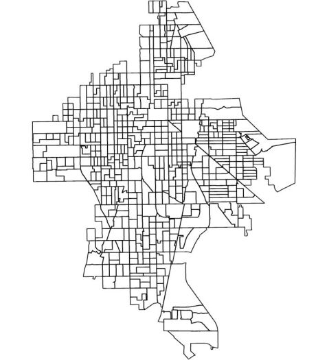
The application on real data concerns the monthly number of burglaries on the south side of Chicago from 2010-2015 (). The counts are registered for the census block groups. The data are taken by Clark and Dixon (2021), https://github.com/nick3703/Chicago-Data. The undirected network structure arises naturally, as an edge between block and is set if the locations share (at least) a border. In this case, the network connection is well-represented by the geographic map of the census blocks in Figure 1. The density of the network is 1.74%. The median degree is 5.
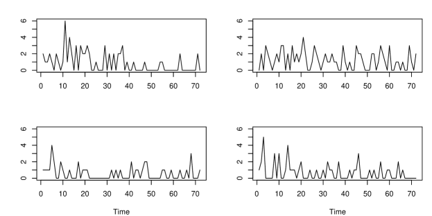
Some time series of burglaries are plotted in Figure 2. The maximum number of burglaries in a month in a census block is 17. We fit the linear and log-linear PNAR(1) and PNAR(2) models. The results are summarized in Tables 3-4. All fitted models produce significant results. The magnitude of the network effects and seems reasonable, as an increasing number of burglaries in a block can lead to a growth in the same type of crime committed in a close area. The lagged effects have a positive impact on the counts. Interestingly, the log-linear model is able to account for the general downward trend registered from 2010 to 2015 for this type of crime in the area analyzed. All the information criteria select the PNAR(2) models, in accordance with the significance of the estimates.
| Linear PNAR(1) | Log-linear PNAR(1) | |||||
| Estimate | SE () | -value | Estimate | SE () | -value | |
| 0.4551 | 2.1607 | 0.01 | -0.5158 | 3.8461 | 0.01 | |
| 0.3215 | 1.2544 | 0.01 | 0.4963 | 2.8952 | 0.01 | |
| 0.2836 | 0.8224 | 0.01 | 0.5027 | 1.2105 | 0.01 | |
| Linear PNAR(2) | Log-linear PNAR(2) | |||||
| Estimate | SE () | -value | Estimate | SE () | -value | |
| 0.3209 | 1.8931 | 0.01 | -0.5059 | 4.7605 | 0.01 | |
| 0.2076 | 1.1742 | 0.01 | 0.2384 | 3.4711 | 0.01 | |
| 0.2287 | 0.7408 | 0.01 | 0.3906 | 1.2892 | 0.01 | |
| 0.1191 | 1.4712 | 0.01 | 0.0969 | 3.3404 | 0.01 | |
| 0.1626 | 0.7654 | 0.01 | 0.2731 | 1.2465 | 0.01 | |
| AIC | BIC | QIC | ||||
|---|---|---|---|---|---|---|
| linear | log-linear | linear | log-linear | linear | log-linear | |
| PNAR(1) | 115.06 | 115.37 | 115.07 | 115.38 | 115.11 | 115.44 |
| PNAR(2) | 111.70 | 112.58 | 111.72 | 112.60 | 111.76 | 112.68 |
We compare the out-sample forecasting performance of the linear PNAR model with versus a baseline STARMA(1,1) model (Pfeifer and Deutrch, 1980), which after some rearrangement is defined as follows
where are independent normal vectors, and , , , are unknown parameters. The Root Mean Square Error (RMSE) obtained by both models is computed. For the PNAR model the RMSE is 0.038 which is less than 0.079 obtained by fitting the STARMA(1,1) model. This shows significant accuracy improvement of the prediction for the PNAR() model. In addition, PNAR avoids estimation of moving average parameters.
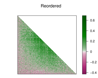
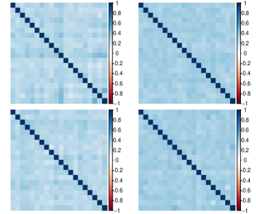
Estimation of the copula is advanced according to the algorithm of Sec. S-9 of the SM. The Gaussian AR-1 copula, described in Sec. 4.1, is compared versus the Clayton copula, over a grid of values for the associated copula parameter, with 100 bootstrap simulations. As a preliminary step for the estimation of Gaussian AR-1 copula we need to reorder the observations for to mimic the structure of the AR-1 copula correlation matrix , where . A coherent ordering for will be the one where the empirical correlation matrix of , say , contains highest correlations close to the main diagonal and then progressively smaller values where the distance from the main diagonal increases. This is a combinatorial problem and for small it is not hard to solve it by trying all the possible orderings. However, when grows, we can recover such ordering by defining the dissimilarity matrix , where is the matrix of ones, and appealing to the concept of anti-Robinson matrix (Hahsler et al., 2008, Sec. 2.1). In this type of matrix, the smallest dissimilarity (largest correlation) values appear close to the main diagonal and the largest dissimilarity (smallest correlation) values appear far from it. Hence, by defining a loss function that quantifies the divergence of a matrix from the anti-Robinson matrix (Hahsler et al., 2008, Sec. 2.2) reordering of the observations is solved by heuristic optimization employing the Anti-Robinson Simulated Annealing (ARSA); see Brusco et al. (2008). The R implementation of the algorithm is easily performed by using the package seriation (Hahsler et al., 2008). The resulting ordering is quite satisfactorily and is plotted in Figure 3 (right) against a random ordering configuration (left).
 |
 |
Using this ordering the Gaussian AR-1 copula is selected 94% and 95% of the times, for the linear and the log-linear PNAR(1) model, respectively. The estimated copula parameter is and , for the linear and log-linear model, respectively, with small standard errors 0.064 and 0.062, correspondingly.
A further estimation step for the PNAR(1) models is performed by applying the two-step GEE estimation method discussed in Sec. S-7. The QMLE estimates are used as starting values of the two-step procedure. An AR-1 working correlation matrix is selected, with as the estimator of the correlation parameter. To compare the relative efficiency of the GEE () versus QMLE (), their bootstrap standard errors have been calculated using 100 simulations by using the estimated copula. We compute the ratio of the standard errors obtained, . The results are and , for the linear and log-liner model, respectively. We note a marginal gain in efficiency from the GEE estimation; this is probably due the a small value of the estimated correlation parameter , which is found to be around 0.008 and 0.005 on average, for linear and log-linear model, respectively. Using different kind of estimator for the correlation parameter might yield significant efficiency improvement but a further study in this direction is needed.
Acknowledgments
This work was completed when M. Armillotta was with the Department of Mathematics & Statistics at the University of Cyprus. We greatly appreciate comments made by two reviewers on an earlier version of the manuscript. Both authors acknowledge the hospitality of the Department of Mathematics & Statistics at Lancaster University, where this work was initiated. This work has been co-financed by the European Regional Development Fund and the Republic of Cyprus through the Research and Innovation Foundation, under the project INFRASTRUCTURES/1216/0017 (IRIDA). In addition, K. Fokianos acknowledges travel support by CY Initiative of Excellence (grant ”Investissements d’Avenir” ANR-16-IDEX-0008), Project ”EcoDep” PSI-AAP2020-0000000013.
Appendix A Appendix
Recall that is a generic constant and is a constant depending on . See also the notation paragraph in the introductory Section 1.
A.1 Proof of Theorem 1
Recall from Zhu et al. (2017, Def. 1) that , where . For each , let be the its truncated -dimensional version. By considering the VAR(1) representation for the PNAR(1) model (2), defined in SM S-1, the process can be rewritten by backward substitution, . For sake of clarity we show the result for the PNAR(1) model. However, the general -lags parallel result extends straightforwardly, by considering the companion VAR(1) representation form (S-1) of the linear PNAR() model. By Proposition 2, it holds that for all and, since , . Similar uniform bounds are obtained for moments of order . For any , , and . Then, by Monotone Convergence Theorem (MCT), exists and is finite with probability 1, moreover is strictly stationary and therefore is strictly stationary, following Zhu et al. (2017, Def. 1). To verify the uniqueness of the solution, take another stationary solution to the PNAR model with finite moments of any order. Then, , where is a constant and , for any and weight . Since is arbitrary, with probability one. ∎
A.2 Proof of Lemma 20
We split the proof accordingly to each single result given in Lemma 20.
A.2.1 Proof of (1)
Define , , , the -th elements of and . Consider the following triangular array , where as . For any , where . We take the most complicated element, , the result is analogously proven for the other elements. Define , and . Additionally, the equality is a consequence of the constructions in Lemma S-2. Then
Set and . By Cauchy-Schwartz inequality, as for and we have that . As a consequence, , by Proposition 2. Moreover, , by the conditional Jensen’s inequality. Similarly, . An application of Lemma S-2 provides . By an analogous recursion argument, it holds that . It is immediate to see that, by Holder’s inequality . In the same way we can conclude that and . Then, by Minkowski inequality
with . By the definition in B1, set . Since is the optimal -measurable approximation to in the -norm and is -measurable, it follows that
where and as , establishing -near epoch dependence (-NED), with , for the triangular array ; see Andrews (1988). Moreover, by a similar argument above, it is easy to see that , by the finiteness of all the moments of the process . Then, using B1 and the argument in Andrews (1988, p. 464), we have that is a uniformly integrable -mixingale. Furthermore, since the law of large number of Theorem 2 in Andrews (1988) provides the desired result as . We only need to show the existence of the matrix H according to (20). Consider the single elements of the matrix :
Note that the linear model (2) can be rewritten has where and is MDS. As ,
| (A-1) |
by assumption B3. The second term
where , as . Define . Then,
| (A-2) | ||||
converges to , as , where the first inequality holds by Minkowski and Jensen’s inequalities, the second inequality is a consequence of and the fourth is deduced by Cauchy inequality. The convergence follows by applying Lemma S-1. Then, as . For the same reason . We move to the following term.
where, as , and . Finally,
as , using B3. So as . For the same reason and . Finally, note that is positive definite, and nonsingular, as is positive definite. ∎
A.2.2 Proof of (2)
For all non-null , the triangular array is a martingale difference array. Moreover, , by Cauchy inequality and the boundedness of all the moments of . Then, is trivially a uniformly integrable -mixingale. An application of Andrews (1988, Thm. 2) provides the result.∎
A.2.3 Proof of (3)
From , we have , where are suitable positive constants. Consider the third derivative
Take the maximum of the third derivatives among to be, for example, at , the proof is analogous for the other derivatives,
Now, define and since all the moment of exist. It is easy to see that as , similarly to the steps of A.2.1 above, with . Then point (3) of Lemma 20 follows by the last limit of B3. We omit the details. ∎
A.3 Proof of Lemma 22
A.3.1 Proof of (1)
Let where and , with , since . We consider again the most complicated element, that is . For , define and , which are the elementwise conditional covariances and correlations, respectively. Then
The second inequality is obtained employing the arguments used for the element of the Hessian as in A.2. Moreover, and . Set . Note that , by the same argument of above. When , , consequently, . Instead, when ,
which is bounded by and the first inequality is a consequence of B4. Then, , we have , where . This entails that
Here again . Then, the triangular array is -NED, with , and Theorem 2 in Andrews (1988) holds for it. This result and B1 yield to the convergence
| (A-3) |
as , for any non-null . The existence of the limiting information matrix (22) follows the same methodology used in A.2.1 for the existence of (20), by considering B3′ instead of B3. The same notation and the same splits for each elements of the information matrix are adopted. So we highlight only the element which is different, i.e. . Clearly, . Moreover, when , , as . When
which converges to , as , following (A-2). ∎
A.3.2 Proof of (2)
Now we show asymptotic normality. Define , and recall the -field . Set , so is a martingale array. By , the Lindberg’s condition is satisfied
for any , as . By the result in equation (A-3)
for any , as . Then, the central limit theorem for martingale array in Hall and Heyde (1980, Cor. 3.1) applies, , and an application of the Cramér-Wold theorem leads to the desired result. ∎
Appendix S Supplementary Material
The supplementary material contains further details on moments of linear and log-linear PNAR models and the proofs of the remaining asymptotic results of the QMLE. A more extended discussion about conditions of Lemma 22 and an empirical exploration of assumptions B2-B4 are also provided. Additional simulation results are presented. A numerical study concerning a more efficient GEE estimator is included. Finally, guidelines for the estimation of the copula and its parameter are discussed.
Recall that is a generic constant and is a constant depending on . See also the notation paragraph in the introductory Section 1.
Appendix S-1 Further results linear PNAR() model
It is easy to derive some elementary properties of the linear PNAR() model. Define . Fix ; we can again rewrite model (3) as a Vector Autoregressive VAR() model
where is a martingale difference sequence, and rearrange it in a -dimensional VAR(1) form by
| (S-1) |
Here we have , , , where is a vector of zeros, and
where is a matrix of zeros.
For model (S-1) we can find the unconditional mean and variance with , where denotes the vec operator and the Kronecker product. For details about the VAR(1) representation of a VAR() model and its moments, see Lütkepohl (2005). Define the selection matrix with dimension . Moreover, note that , where the first equality follows by and the second one is true since , by construction, and so ; the iteration of this argument times gives the result. Then, the following proposition holds.
Proposition S-1.
Applying these results to model (1) (equivalently (2)), we obtain
| (S-2) | ||||
where . The mean of depends on the network effect and the momentum effect but not on the structure of the network; this is true in the case the covariates are not present (Zhu et al., 2017, Case 1). By contrast, the network structure always has an impact (through ) on the second moments; in addition, the conditional covariance shows that it depends on the copula correlation. Equations (S-2) are analogous to equations (2.4) and (2.5) of Zhu et al. (2017, Prop. 1), who studied the continuous variable case. Then, the interpretations (Case 1 and 2 pp. 1099-1100) and the potential applications (Section 3, p. 1105) apply also here for integer-valued case.
S-1.1 Proof of Proposition 2
For clarity in the notation, we present the result for the PNAR(1) model, but it can be easily to the case . By and (S-2), we have that for all . Then, and , using properties of monotone bounded functions. Moreover, , employing Poisson properties, where are the Stirling numbers of the second kind. Set . For the law of iterated expectations, we have that
where the last inequality follows for the stationarity of the process and the finiteness of its moments, with fixed . As is bounded by , for the same reason above . Since , similarly as above
where the second inequality holds because of the conditional Jensen’s inequality, and so on, for , the proof works analogously by induction and therefore is omitted. ∎
S-1.2 Empirical properties of the linear PNAR(1) model
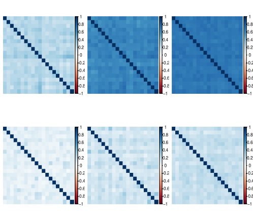
To gain intuition for model (1), we simulate a network from the stochastic block model (Wang and Wong, 1987); see Figure S-1. Moments of the linear model (1) exist and have a closed form expression; see (S-2). The mean vector of the process has elements which vary between 0.333 to 0.40, for whereas the diagonal elements of take values between 0.364 and 0.678. We take this simulated model as a baseline for comparisons and its correlation structure is shown in the upper-left plot of Figure S-1. The top-right panel displays the same information but for the case of increasing activity in the network. The bottom panel of the same figure shows the same information as the upper panel but with a more sparse network, i.e. . Increasing the number of relationships among nodes of the network boosts the correlation among the count processes. A more sparse structure of the network does not appear to alter the correlation properties of the process though.
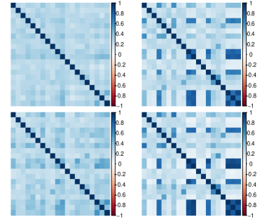
Figure S-2 shows a substantial increase in the correlation values which is due to the choice of the copula parameter. Interestingly, the intense activity of the network increases the correlation values of the count process. This aspect may be expected in real applications. For the Clayton copula (see lower plots of the same figure) we observe the same phenomenon but the values of the correlation matrix are lower when compared to those of the Gaussian copula. We did not observe any substantial changes for the marginal mean and variances.
Figure S-3 shows the impact of increasing network and momentum effects. We observe that the network effect is prevalent, as it can be seen from the top-right panel which also shows the block network structure. Significant inflation for the correlation can be also noticed when increasing the momentum effect (bottom-left panel). When increasing the network effect the marginal means vary between 0.333 to 1 and have large variability within the nodes; this is a direct consequence of the block network structure. When increasing the momentum effect, the marginal means take values from 0.5 to 0.667. When both effects grow, the mean values increase and are between 0.5 and 2.
Appendix S-2 Further results for log-linear PNAR() model
S-2.1 Proof of Proposition 4
For simplicity set . Since is approximately MDS and , an approximated version of Proposition S-1 holds for in (9), with suitable adjustments. Then, , and a first order Taylor approximation provides , for all . By assuming the existence of moments of order , i.e. , we can obtain a more accurate approximation of polynomial order . From the approximation above, and then , for all . The existence of the latter moments allows to perform a Taylor approximation for the function of any arbitrary order on , around its mean, leading to the conclusion , . ∎
S-2.2 Proof of Theorem 2
By Proposition 3, is strictly stationary, for any and all the moments of exist by Proposition 4. Then, and exists with probability one and is stationary. Hence, is strictly stationary, following Zhu et al. (2017, Def. 1). To prove the uniqueness of the solution, note that the proof of Theorem 1 applies to , by suitable adjustments, such as, . Therefore, is strictly stationary, in the sense of Zhu et al. (2017, Def. 1), and unique stationary solution to the log-linear PNAR model. The same holds for the process since it is a one-to-one deterministic function of the unique solution. ∎
S-2.3 Empirical properties of the log-linear PNAR(1) model
We give here some insight on the structure of the model (6). Here an explicit formulation of the unconditional moments is not possible for the count process . We report the sample statistics to estimate the unknown quantities and replicate the same baseline characteristics and the same scenarios of the linear case. In Figure S-4 we can see that, analogously to the linear case, the correlations among counts grow when more activity in the network is showed. However, here a more sparse matrix seems to slightly affect correlations. The general levels of correlations are higher than the linear case in Figure S-1. The mean ranges around 1.7 and 2; it tends to rise with higher network activities up to 2.2. For the variance we find analogous results.
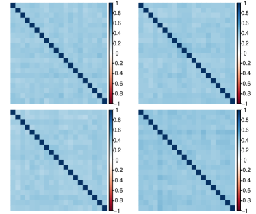
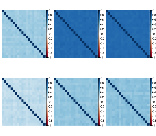
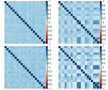
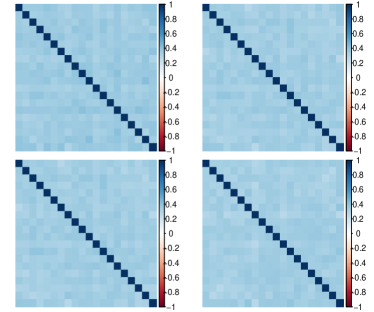
Figure S-5 shows the outcomes obtained by varying the copula structure and the copula parameter . The results are similar to Figure S-2 but here the correlations tend to be more homogeneous. By adding positive weights to the network and momentum effect in Figure S-6 we notice comparable results with those of the linear model in Figure S-3, but here the growth in parameters leads to a less severe effect on correlations. Significant increases in mean and variance are detected. In the log-linear model negative values for the parameters are allowed. In Figure S-7 we see no remarkable impact of negative coefficients on correlations. However, the sample means and variances decrease when compared to the corresponding plots produced using .
Appendix S-3 Additional proofs on the asymptotic properties of QMLE
S-3.1 Preliminary Lemmas
Lemma S-1.
For model (2) assume and that the conditions B2 hold. Then, there exists such that for any integer , where , is a constant and is defined in B2.1. Moreover, for integers and ,
Proof.
The proof of Lemma S-1 follows the same line of arguments of Zhu et al. (2017, Supp. Mat. pp. 6-8). Here, we show only the parts that are different. Set . The same can be easily proved for the other values. By B2.1 and Lemma 2 in Zhu et al. (2017), with the same notation, note that and where . With , it holds the inequality , then we need to prove the limit , which is equivalent to show . The expansion of the matrix provides . Note that , with . So,
using Cauchy-Schwartz inequality. This means one just needs to prove
| (S-3) |
For the first term of (S-3), by applying the spectral decomposition on we have , which is a diagonal quadratic form, where is an orthogonal matrix whose columns are orthonormal eigenvectors of and is a diagonal matrix with its eigenvalues. Then, for Cauchy inequality, it holds that , for B2.1. By Raleigh-Ritz theorem (Seber, 2008, 6.58), the second term is bounded as follow
where the second inequality is due to Zhu et al. (2017, Supp. Mat., p. 7), with and the convergence follows by B2.2. ∎
Lemma S-2.
Rewrite the linear model (2) as , for where and . Define the following predictors, for :
where and . Let and with . Then,
where .
Proof.
Set ,
The first inequality holds for an application of the multivariate mean value theorem. Moreover, recall that and . Now set ,
and the last inequality comes from the previous recursion. It is immediate to see that, for , . ∎
S-3.2 Proof of Lemma 25
The proof is analogous to that of Lemmas 20-22. We will point out only the parts which differ substantially.
Lemma S-3.
Proof.
The proof is analogous to Lemma S-2 and therefore is omitted. ∎
S-3.2.1 Proof of (1)
Set , , . Consider the triangular array , where as . For any , . Then,
where and . The second inequality follows by and , for . Set and . It is easy to show that , by Cauchy-Schwartz inequality. Moreover, and . All these quantities are bounded by Proposition 4. Similarly to the linear model, Lemma S-3 entails , where is a constant, . Similarly, are bounded. Similarly to the Proof of Proposition 4, the existence of the latter moments allows to perform a Taylor approximation for the function of any arbitrary order on , around its mean, leading to , , and . Then, is -NED and, by Assumption B1L, the conclusion follows as for the linear model. The proof of existence of the matrix in (25), follows by B2L and is a special case of the existence of the matrix , showed in the next point.∎
S-3.2.2 Proof of (2)
Let , where , with , since . Working analogously as before
where , and , where , for B4L, similarly to the linear model, proving -NED. We prove the existence of the matrix as in (25), using the properties of the network (B2L). , as , by B3L. , where and , where , by B3L, and , by B2L, similarly to the linear model, as . , where , , and finally , by, B3L, as . The other elements follow similarly. The proof of asymptotic normality is established in the same fashion of the linear model and therefore is omitted.∎
S-3.2.3 Proof of (3)
Consider the third derivative
Take, for example, the case ,
The rest of the proof can be derived analogously to the proof of Lemma 20. We omit the details.∎
S-3.3 Proof of Theorem 3
Recall the quasi log-likelihood (10) and set a compact neighborhood of , for any . If lies between and , a Taylor expansion gives
where , , where denotes the minimum eigenvalue of a matrix, and , as , by an application of mean value theorem and Lemma 20. By the continuous mapping theorem and Lemma 20 we have that . Moreover, by Lemma 22. By combining all the above and following Fokianos and Tjøstheim (2012, Proof of Thm. 1, p. 1224) we obtain that there exists, with probability tending to one, a solution to the system , denoted by , in the interior of . Since all elements of (12) are positive, we have , for any non null . Then, is unique solution in the interior of . The same argument applies for any , i.e. there exists with probability tending to one a solution to the score equations in . But is the unique solution to the score equations in and therefore lies in with probability tending to one. Then is consistent. The asymptotic normality follows by a Taylor expansion of the score and Lemmas 20-22. We omit the details. ∎
S-3.4 Proof of Theorem 5
For any deterministic non-null vector , , by the consistency of the QMLE (Theorem 3) and the continuous mapping theorem (CMT); this result coupled with condition 1 in Lemma 20, provides . For the information matrix, note that , where, by Theorem 3 and CMT, it holds that , similarly as above. Now consider . Define , the triangular array , where and are the single summands of (13) and (26), respectively. Furthermore, set , so that, in (13), . One can easily see that
is a martingale difference array and, since , by the results of Theorem 3, the sequence is a uniformly integrable -mixingale. By Andrews (1988, Thm. 2), as (and ); consequently . Finally, , as it is identical to the result of Lemma 22-(1). An application of Slutsky’s lemma yields the result. The proof is analogous for the log-linear model (7), therefore is omitted. ∎
S-3.5 Proof of Corollary 1
Appendix S-4 Empirical verification of assumptions B2-B3
This section illustrates some numerical evidence verifying the network condition B2 and the convergence of the limits assumed in B3-B3′. Starting from B2.1, a sufficient condition for both irreducibility and aperiodicity of the Markov chain, whose states are the nodes of the network , is that the network is always fully connected after a finite number of steps. Moreover, in B2.2, a sufficiently slow diverging rate of is required. These results have already been verified empirically in Zhu et al. (2017, Supp. Mat., Sec. 7), therefore they are omitted here. The remaining conditions to be verified for B2 are i) , for some , and ii) as ; where is the stationary distribution of the Markov chain defined in B2.1, . To this aim, we consider the same simulation setting of Sec. 4.1, with the copula parameter , , and . The number of simulations is . Condition i) requires that , where recall that is a generic constant. We approximate by using the sample counterpart and compute the maximum eigenvalue, to obtain , for various values of . The experiment is replicated times for , whose values are box-plotted in the left plot of Figure S-8, with ; we observe that its values are well bounded by a positive constant, when grows. We obtain similar results for . When , the approximation improves. Once i) is verified, condition ii) is satisfied provided that converges to 0 faster than , say , where . Then, ii) will be equivalent to show that . The second boxplot in Figure S-8, shows that this is indeed the case, when is increasing, for example, with .
Regarding the limit convergence assumptions specified by B3-B3′, a similar numerical verification as above can be studied. We consider the most complex element , where is substituted by the empirical counterpart, , where , then ; analogous results can be derived for the other cases. The values of computed over 500 simulations are box-plotted in the right graph of Figure S-8. As becomes larger, we see the assumed convergence.
Similar empirical studies have been performed also for the log-linear model (7), for B2L-B3L, with obvious rearrangement of the notation. The results are plotted in Figure S-9 and analogous comments hold. Moreover, all the results are in line to what was found in the special case of OLS, with , and reported by Zhu et al. (2017, Supp. Mat., Sec 7).
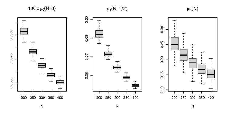
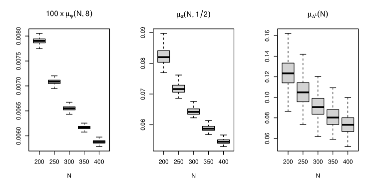
Appendix S-5 Further results for assumption B4
The condition (21) in assumption B4 depends on the copula construction specified on the exponential waiting times of the data generating process discussed in Section 2.1. This structure of dependence, in turn, is transferred to the generated conditional Poisson random variables , through a non-deterministic transformation. While the copula is invariant to one-to-one deterministic transformations, we do not have such a transformation in this case. Then, it is not clear how to establish the form of the conditional covariance (and correlation) of the counts, and so assumption B4 cannot be addressed theoretically. However, this problem appears in other settings. Indeed, similar difficulties arise even in alternative frameworks, like imposing the copula construction directly on Poisson (conditional) marginals, see the discussion by Inouye et al. (2017), among others. Furthermore, direct joint multivariate count distributions implicitly introduce strong constraints to the correlation structure of the counts. For instance the multivariate conditional Poisson distribution described in Fokianos (2022, Sec. 2.1), has the property , , with being a constant parameter.
It is still possible to give an empirical evidence where B4 is satisfied. For example, suppose the selected copula is Gaussian, with AR-1 correlation matrix, as specified in Sec. 4.1. Recall that the correlation matrix of such copula has single element . Clearly, by fixing , for example, and , we obtain a geometrically decaying pattern of correlations. However, do not correspond to correlations of the observed count random variables, nor represent the correlations of the exponential inter-arrival times, in general. Then, we want to explore the impact of the copula correlation coefficients on the correlations of the conditional exponential random variables first, and, in turn, on the conditional Poisson ones. In this empirical study the network structure is given by the Erdős-Rényi Model (ER), but analogous results were obtained for the SBM of Example 1, with , and therefore are omitted.
Example S1.
Figure S-10 shows the results of a simulation study on the theoretical copula correlations specified versus the mean of empirical pairwise correlations, for the exponential random variables , with , obtained by averaging out the correlations matrices along the simulations. The correlation structure of the copula appears to be essentially transferred to the correlations of the exponential waiting times. Figure S-11 depicts, instead, the resulting mean empirical pairwise correlations of the conditional Poisson random variables , obtained from simulations. As expected, the correlation structure of the conditional exponential random variables does not correspond to the correlation structure of the conditional Poisson ones. However, when magnitudes of the network () and autoregressive () effects are not too large, a detected decaying pattern towards zero of the empirical correlations is still inherited by the counts. This means that a non increasing sequence , such that , satisfying (21), can always be found for the correlations of the conditional Poisson variables. For example, the orange line in Table S-11, shows the graph of , which clearly satisfies B4. Similar outcomes, not presented here, have been found for the Student’s t copula, with 2 and 10 degrees of freedom.
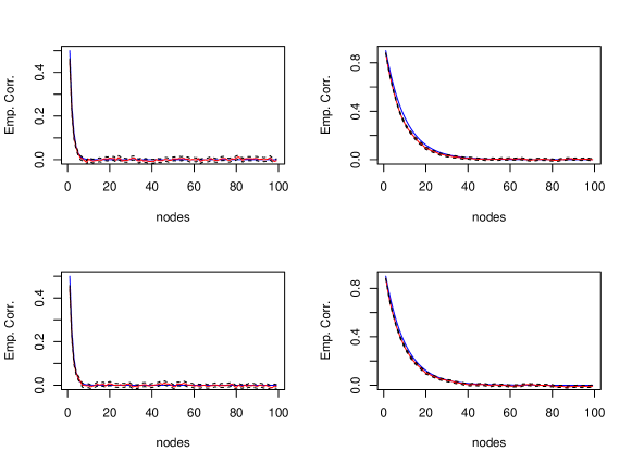

Appendix S-6 Additional details about Lemma 22
Define the normalized random process , so , such that and . Recall (21), for , which can be rewritten as . Consider the following assumption.
-
B5
The sequence defined in B4 is such that and, for , almost surely
Proposition S-2.
Proof.
Note that , where the last equality follows for the Poisson third central moment. Recall that , where . Then,
where is a universal constant and the inequality follows by an application of Yaskov (2015, Thm. 2.1) with conditional expectation. Define . So which is the Hessian matrix squared (up to a constant), and it can be shown to be uniformly bounded, by standard Cauchy inequalities and the boundedness of all the moments of . ∎
Appendix S-7 Improving efficiency of QMLE
We have developed a complete theoretical framework for QMLE inference. However, in general, the QMLE is computed under the independence assumption and therefore it will suffer efficiency loss. The lack of efficiency might become large especially when large correlations among the count processes are present. Some empirical evidence regarding this problem has been found in numerical studies of Sec. 4.1 and S-8. Since, in practice, the dependence structure among the integer-valued random variables is modeled through a copula, with a parameter , the problem can be intuitively viewed on examining the performance of the QMLE when the copula parameter takes large values. We propose here a two-step Generalized Estimating Equation (GEE) procedure, originally introduced for longitudinal data analysis (Zeger and Liang, 1986), which adds a further estimation step to the previous QMLE methodology. Consider model (4), for example. The proposed QMLE maximizing the quasi log-likelihood (10) is the -dimensional vector of unknown parameter which solves the system of equation , where is defined in (11). The GEE estimator will be then the vector of roots of the following system.
| (S-4) |
where and is an matrix, the so called working correlation matrix, depending on a correlation parameter . The matrix is specified by the researcher and it will not necessarily reflect the true contemporaneous correlation structure of the multivariate process , which in fact depends on the copula and whose analytical form is not available. Moreover, the working correlation matrix should not be confused with the copula correlation matrix which is specified on elliptical copulas, see for example Sec. 4.1, as the two matrices can be, in general, different.
Note that the QMLE can be obtained as a particular case of (S-4), when , recovering the score function (11). Intuitively, the estimator obtained by (S-4), which incorporates a correlation structure among multivariate process , by introducing the matrix , is expected to explain a larger part of the variability connected to the process of study. Therefore, (S-4) should lead to improved efficiency results, compared to the QMLE with independence likelihood (10). In summary, we propose the following two-step GEE estimator.
-
1.
Compute the QMLE of model (4). Then choose and compute .
-
2.
Estimate from (S-4), with working correlation .
There are two issues: i) choosing a suitable form for the working correlation matrix, among several available alternatives; see for example Pan (2001, p. 121), ii) find a suitable estimator for the parameter . For problem i), we note the following. Since the network dimension may be large, the inversion of the matrix may be extremely expensive and, ultimately, computationally unfeasible. Furthermore, since only the inverse of such matrix would be required by the proposed estimating equations, we suggest to find a correlation structure where an analytical form for the inverse is known. For example, in this work we decide to impose the AR-1 correlation structure where , for and . Such working correlation matrix is appealing since it has an analytical form of the inverse, i.e. , where is a tridiagonal matrix, with the main diagonal consisting of the elements of the vector ), and the remaining two diagonals are the elements of the vector of ; see Sutradhar and Kumar (2003, eq. 1.1). The estimation of the correlation parameter is usually performed using moment estimators (Zeger and Liang, 1986, Sec. 4). We select two estimators, and , where
| (S-5) |
are the empirical Pearson correlations from the quasi-likelihood estimation.
To check the performance of the two-step GEE estimator we run a simulation study, by generating data from model (2) using the same setting of the simulation study outlined in Sec. 4.1; data are produced by employing a copula parameter selected by an equidistant grid of values in the interval . Then, we compare the estimation performances of the QMLE versus the GEE, by measuring their relative efficiency, with the relative Mean Square Error, , where is the number of simulations performed and is the estimator associated with the replication . Clearly, shows improved efficiency of when compared to . The same comparison can be done marginally for each parameter of the model , for . The results of the Monte Carlo simulations are summarized in Figure S-12.
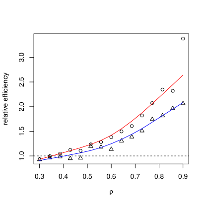
When the data are generated with a moderate or strong correlation (copula parameter ) the GEE is relatively more efficient than the QMLE. The improvement in efficiency is larger as the correlation becomes stronger and tends to grow even by increasing network and time size (). This would be expected since the QMLE becomes a poor approximation of the true likelihood as the dependence structure of the multivariate count process becomes stronger, whereas the specified GEE methodology appears to be able to account for a significant part of the correlations among the counts, even though the working correlation does not reflect the true correlation structure of the data. Similar results are obtained by comparing the marginal efficiencies , with , therefore are omitted. The employment of the moment estimator gave analogous results but with gain in efficiency less than the gain obtained by used . The results of the current section can be established similarly for the log-linear version of the model.
Although the result of the present simulation study are encouraging, the problem of improving the efficiency of the QMLE is only at the initial stage and further studies are required. For example, alternative working correlation structures may be used, like the equicorrelation structure (EQC), , where is a matrix of ones and an equal pairwise correlation is assigned to all the possible couples of the multivariate time series. This matrix also have analytical inverse, , where and . For a proof see Rao (2002, p. 67); moreover, more complex correlation structures could be considered. In addition, further estimators for the correlation parameter may be available. Finally, the development of an asymptotic theory for the proposed GEE estimator would be of interest. Such extensions will be studied in a future contribution.
Appendix S-8 Additional simulation results
We present here further comments and findings from the simulation study reported in Sec. 4.1. The same parameter values have been used as in Sec. 4.1. In the situation of independence () the QMLE reduces to the standard MLE. When is big and is small we see that QMLE provides satisfactory results (Table S-2, S-4). However, this is not always the case. Following the results of Sec. 4.1 and when , a more complex structure of dependence among variables will be observed. Therefore the quasi likelihood (10) can be thought as a crude approximation to the true likelihood. In particular, when and is small, care must be taken in the interpretation of QMLE. This fact is also confirmed by the Tables S-1 and S-3 which illustrate slightly poorer results in the case of strong dependence among counts. Finally, if both the temporal size and the network size are reasonably large, then inferential results in Section 3 are confirmed.
Figure S-14 shows a QQ-plot of the standardized estimators for the log-linear model of order 1, with Gaussian copula () and . When both dimensions are large, then the approximation is satisfactory. Clearly, by reducing dependence among count variables, we can obtain better large-sample approximations but these results are not plotted due to space constraints.
| Dim. | IC | |||||||||||
|---|---|---|---|---|---|---|---|---|---|---|---|---|
| 20 | 100 | 0.202 | 0.295 | 0.194 | 0.198 | 0.290 | 0.189 | 0.012 | 0.008 | 85.3 | 93.3 | 94.0 |
| (0.032) | (0.052) | (0.040) | (0.034) | (0.005) | (0.042) | (0.042) | (0.031) | |||||
| 100 | 100 | 99.6 | 100 | 100 | 99.3 | 1.8 | 1.5 | |||||
| 200 | 0.202 | 0.295 | 0.198 | 0.198 | 0.291 | 0.195 | 0.010 | 0.006 | 83.4 | 93.6 | 94.2 | |
| (0.024) | (0.042) | (0.029) | (0.025) | (0.043) | (0.030) | (0.035) | (0.022) | |||||
| 100 | 100 | 100 | 100 | 100 | 100 | 1.8 | 1.7 | |||||
| 100 | 20 | 0.209 | 0.271 | 0.195 | 0.202 | 0.262 | 0.191 | 0.018 | 0.010 | 80.7 | 85.6 | 93.5 |
| (0.045) | (0.079) | (0.047) | (0.050) | (0.083) | (0.048) | (0.074) | (0.037) | |||||
| 99.8 | 88.9 | 98.5 | 99.8 | 86.4 | 97.4 | 1.9 | 1.5 | |||||
| 50 | 0.203 | 0.291 | 0.196 | 0.198 | 0.285 | 0.193 | 0.013 | 0.007 | 78.3 | 87.4 | 94.4 | |
| (0.028) | (0.053) | (0.030) | (0.031) | (0.055) | (0.031) | (0.048) | (0.023) | |||||
| 100 | 100 | 100 | 100 | 100 | 100 | 1.5 | 1.6 | |||||
| 100 | 0.202 | 0.294 | 0.199 | 0.198 | 0.290 | 0.197 | 0.009 | 0.004 | 80.0 | 89.6 | 95.2 | |
| (0.020) | (0.037) | (0.021) | (0.022) | (0.038) | (0.022) | (0.033) | (0.016) | |||||
| 100 | 100 | 100 | 100 | 100 | 100 | 1.1 | 1.4 | |||||
| 200 | 0.201 | 0.298 | 0.199 | 0.199 | 0.295 | 0.197 | 0.008 | 0.004 | 73.8 | 87.7 | 93.0 | |
| (0.014) | (0.026) | (0.015) | (0.015) | (0.027) | (0.016) | (0.023) | (0.011) | |||||
| 100 | 100 | 100 | 100 | 100 | 100 | 1.7 | 1.4 | |||||
| Dim. | IC | |||||||||||
|---|---|---|---|---|---|---|---|---|---|---|---|---|
| 20 | 100 | 0.200 | 0.299 | 0.198 | 0.196 | 0.294 | 0.195 | 0.012 | 0.007 | 94.7 | 99.6 | 94.0 |
| (0.015) | (0.037) | (0.026) | (0.017) | (0.038) | (0.027) | (0.035) | (0.022) | |||||
| 100 | 100 | 100 | 100 | 100 | 100 | 2.0 | 2.1 | |||||
| 200 | 0.200 | 0.299 | 0.199 | 0.197 | 0.296 | 0.197 | 0.008 | 0.006 | 93.5 | 99.6 | 92.9 | |
| (0.011) | (0.023) | (0.018) | (0.012) | (0.024) | (0.019) | (0.021) | (0.015) | |||||
| 100 | 100 | 100 | 100 | 100 | 100 | 2.4 | 2.8 | |||||
| 100 | 20 | 0.202 | 0.297 | 0.198 | 0.195 | 0.291 | 0.195 | 0.016 | 0.008 | 95.2 | 97.5 | 93.2 |
| (0.021) | (0.046) | (0.025) | (0.025) | (0.048) | (0.026) | (0.043) | (0.021) | |||||
| 100 | 100 | 100 | 100 | 100 | 100 | 2.9 | 3.1 | |||||
| 50 | 0.200 | 0.299 | 0.200 | 0.196 | 0.296 | 0.198 | 0.010 | 0.005 | 95.0 | 99.5 | 94.5 | |
| (0.013) | (0.029) | (0.016) | (0.016) | (0.030) | (0.016) | (0.028) | (0.014) | |||||
| 100 | 100 | 100 | 100 | 100 | 100 | 2.8 | 2.0 | |||||
| 100 | 0.201 | 0.298 | 0.200 | 0.197 | 0.296 | 0.198 | 0.008 | 0.003 | 94.8 | 99.6 | 94.7 | |
| (0.009) | (0.021) | (0.012) | (0.011) | (0.022) | (0.012) | (0.020) | (0.010) | |||||
| 100 | 100 | 100 | 100 | 100 | 100 | 2.3 | 2.0 | |||||
| 200 | 0.200 | 0.300 | 0.200 | 0.198 | 0.298 | 0.199 | 0.006 | 0.002 | 94.7 | 99.9 | 94.7 | |
| (0.006) | (0.015) | (0.008) | (0.008) | (0.015) | (0.008) | (0.014) | (0.007) | |||||
| 100 | 100 | 100 | 100 | 100 | 100 | 2.1 | 2.4 | |||||
| Dim. | IC | |||||||||||
|---|---|---|---|---|---|---|---|---|---|---|---|---|
| 20 | 100 | 0.207 | 0.291 | 0.197 | 0.212 | 0.293 | 0.199 | -0.007 | -0.002 | 54.9 | 76.3 | 81.8 |
| (0.104) | (0.061) | (0.049) | (0.118) | (0.062) | (0.051) | (0.061) | (0.048) | |||||
| 51.8 | 99.4 | 97.9 | 42.8 | 99.3 | 97.0 | 3.8 | 2.4 | |||||
| 200 | 0.204 | 0.296 | 0.197 | 0.209 | 0.298 | 0.198 | -0.003 | -0.007 | 48.6 | 78.9 | 85.6 | |
| (0.073) | (0.044) | (0.039) | (0.082) | (0.050) | (0.039) | (0.050) | (0.037) | |||||
| 78.6 | 100 | 100 | 72.0 | 100 | 100 | 2.2 | 1.9 | |||||
| 100 | 20 | 0.233 | 0.265 | 0.200 | 0.252 | 0.271 | 0.202 | -0.025 | -0.006 | 37.9 | 48.5 | 77.9 |
| (0.146) | (0.110) | (0.058) | (0.168) | (0.112) | (0.059) | (0.109) | (0.057) | |||||
| 37.6 | 66.5 | 91.8 | 32.9 | 65.7 | 91.5 | 2.8 | 3.4 | |||||
| 50 | 0.213 | 0.289 | 0.198 | 0.218 | 0.291 | 0.199 | -0.007 | -0.002 | 37.3 | 58.4 | 83.5 | |
| (0.089) | (0.063) | (0.038) | (0.103) | (0.066) | (0.038) | (0.065) | (0.037) | |||||
| 65.1 | 99.1 | 100 | 55.0 | 98.7 | 100 | 1.8 | 3.1 | |||||
| 100 | 0.207 | 0.294 | 0.199 | 0.212 | 0.296 | 0.199 | -0.007 | -0.001 | 35.2 | 62.7 | 84.3 | |
| (0.066) | (0.050) | (0.026) | (0.078) | (0.051) | (0.027) | (0.051) | (0.026) | |||||
| 87.4 | 100 | 100 | 76.6 | 100 | 100 | 1.7 | 2.4 | |||||
| 200 | 0.204 | 0.297 | 0.199 | 0.206 | 0.298 | 0.200 | -0.004 | 0.000 | 39.4 | 67.2 | 84.3 | |
| (0.046) | (0.034) | (0.019) | (0.053) | (0.036) | (0.019) | (0.035) | (0.019) | |||||
| 99.1 | 100 | 100 | 100 | 96.8 | 100 | 1.9 | 2.5 | |||||
| Dim. | IC | |||||||||||
|---|---|---|---|---|---|---|---|---|---|---|---|---|
| 20 | 100 | 0.201 | 0.299 | 0.200 | 0.202 | 0.299 | 0.200 | 0.000 | -0.001 | 87.1 | 98.9 | 86.1 |
| (0.044) | (0.034) | (0.032) | (0.050) | (0.039) | (0.032) | (0.039) | (0.031) | |||||
| 99.5 | 100 | 100 | 97.8 | 100 | 100 | 2.7 | 2.7 | |||||
| 200 | 0.202 | 0.299 | 0.199 | 0.203 | 0.298 | 0.199 | 0.001 | -0.002 | 86.1 | 99.2 | 85.8 | |
| (0.031) | (0.024) | (0.022) | (0.036) | (0.028) | (0.023) | (0.029) | (0.022) | |||||
| 100 | 100 | 100 | 100 | 100 | 100 | 3.0 | 1.7 | |||||
| 100 | 20 | 0.206 | 0.294 | 0.199 | 0.207 | 0.294 | 0.199 | 0.000 | -0.001 | 85.6 | 94.5 | 81.8 |
| (0.075) | (0.068) | (0.032) | (0.088) | (0.069) | (0.032) | (0.064) | (0.031) | |||||
| 76.3 | 98.3 | 100 | 66.2 | 98.6 | 100 | 3.6 | 4.1 | |||||
| 50 | 0.203 | 0.298 | 0.199 | 0.203 | 0.298 | 0.199 | -0.001 | 0.000 | 84 | 98.3 | 82.7 | |
| (0.047) | (0.042) | (0.020) | (0.058) | (0.043) | (0.020) | (0.041) | (0.020) | |||||
| 98.9 | 100 | 100 | 92.5 | 100 | 100 | 3.3 | 4.2 | |||||
| 100 | 0.203 | 0.298 | 0.200 | 0.204 | 0.298 | 0.200 | -0.001 | 0.000 | 86.9 | 99.5 | 85.1 | |
| (0.033) | (0.029) | (0.014) | (0.041) | (0.030) | (0.014) | (0.029) | (0.014) | |||||
| 100 | 100 | 100 | 99.9 | 100 | 100 | 2.7 | 2.6 | |||||
| 200 | 0.200 | 0.299 | 0.200 | 0.201 | 0.299 | 0.200 | -0.001 | 0.000 | 87.2 | 99.5 | 86.6 | |
| (0.023) | (0.021) | (0.010) | (0.029) | (0.021) | (0.010) | (0.021) | (0.010) | |||||
| 100 | 100 | 100 | 100 | 100 | 100 | 2.5 | 2.5 | |||||


It can be seen that the conclusions of the simulation study hold true even when the number of network nodes is big and eventually . See Table S-5.
We present here an additional simulation result obtained using a spatial network (Table S-6). The network is generated by first-order spatial ordering neighbor structure as defined in Pfeifer and Deutsch (1980, Fig. 1). In this construction each node is connected in a spatial network to the nodes that are immediately adjacent to it. The mean of estimated coefficients is basically equal to the true values, the standard errors in brackets are small and the coefficient are significantly different from 0 on the 100% of replications providing results comparable to the other network models.
| Dim. | Parameters | |||
|---|---|---|---|---|
| 500 | 200 | 0.200 | 0.299 | 0.200 |
| (0.007) | (0.015) | (0.009) | ||
| 100 | 100 | 100 | ||
| 1000 | 200 | 0.200 | 0.300 | 0.200 |
| (0.004) | (0.010) | (0.003) | ||
| 100 | 100 | 100 | ||
| Dim. | Parameters | |||
|---|---|---|---|---|
| 100 | 100 | 0.200 | 0.299 | 0.199 |
| (0.008) | (0.018) | (0.011) | ||
| 100 | 100 | 100 | ||
| 200 | 200 | 0.200 | 0.300 | 0.200 |
| (0.004) | (0.009) | (0.005) | ||
| 100 | 100 | 100 | ||
Appendix S-9 Copula estimation
We propose an heuristic parametric bootstrap algorithm for both identification of the copula structure and estimation of the unknown copula parameter . We consider the case of a copula which depends on a univariate parameter.. A thorough study of the problem will be discussed elsewhere. The methodology is based on parametric bootstrap and it is outlined below:
-
1.
Given the observations, , estimate .
-
2.
For a given a copula structure and for a given value of the copula parameter, generate a sample of conditional marginal Poisson counts, , with the algorithm introduced in Sec. 2.1, using the estimates from step 1.
-
3.
Compute the weighted mean absolute error (WMAE) .
-
4.
Repeat step 2-3 for different copula structure and over a grid of values for the copula parameter. Estimate the copula and its parameter by , as those choices which minimize the WMAE.
-
5.
Repeat steps 2-4 for times, where , to select the copula structure and parameter value minimizing the WMAE, giving the realizations . The chosen copula structure is the one that is selected most of the times. The final estimate of the copula parameter is the average of copula parameters for such realizations (computed by only considering the realizations of the copula structure that is selected most of the times). Similarly, the associated standard error are computed only from these realizations.
We run a small simulation study to show the effectiveness of the proposed estimation algorithm. The network is obtained from the SBM model presented in Ex. 1, with blocks. We set , and . Data are generated by linear and log-linear PNAR(1) models as in (2),(7), respectively, by using the algorithm of Section 2.1, with a Gaussian AR-1 copula structure, as described in Sec. 4.1, where the true value of the copula parameter is . We run the bootstrap algorithm, with , comparing the Gaussian AR-1 copula and the Clayton copula. The parameters are picked on a grid of 17 equidistant values in the interval (0.1,0.9) for the Gaussian copula parameter, and (0.5,8) for the Clayton one. The results are summarized in Table S-7. The third row indicates the percentage selection of the right copula structure (Gaussian AR-1); we see that the right copula structure is selected the vast majority of the times, for both models. Within these realizations the obtained estimate for the copula parameter, displayed in the first row, is quite accurate (for both models). Finally the second row shows that the associated standard errors are quite small and confirm the significance of the estimates.
References
- Ahmad (2016) Ahmad, A. (2016). Contributions à l’éconemétrie des séries temporelles à valeurs entières. Ph. D. thesis, University Charles De Gaulle-Lille III, France.
- Ahmad and Francq (2016) Ahmad, A. and C. Francq (2016). Poisson QMLE of count time series models. Journal of Time Series Analysis 37, 291–314.
- Aknouche and Francq (2021) Aknouche, A. and C. Francq (2021). Two-stage weighted least squares estimator of the conditional mean of observation-driven time series models. Journal of Econometrics, To appear.
- Al-Osh and Alzaid (1987) Al-Osh, M. and A. A. Alzaid (1987). First-order integer-valued autoregressive (INAR (1)) process. Journal of Time Series Analysis 8, 261–275.
- Alzaid and Al-Osh (1990) Alzaid, A. and M. Al-Osh (1990). An integer-valued pth-order autoregressive structure (INAR (p)) process. Journal of Applied Probability, 314–324.
- Andreassen (2013) Andreassen, C. M. (2013). Models and inference for correlated count data. Ph. D. thesis, Aaarhus University, Denmark.
- Andrews (1988) Andrews, D. W. (1988). Laws of large numbers for dependent non-identically distributed random variables. Econometric Theory 4, 458–467.
- Armillotta et al. (2022) Armillotta, M., A. Luati, and M. Lupparelli (2022). Observation-driven models for discrete-valued time series. Electronic Journal of Statistics 16, 1393–1433.
- Bracher and Held (2020) Bracher, J. and L. Held (2020). Endemic-epidemic models with discrete-time serial interval distributions for infectious disease prediction. International Journal of Forecasting, in press.
- Brusco et al. (2008) Brusco, M. J., H.-F. Köhn, and S. Stahl (2008). Heuristic implementation of dynamic programming for matrix permutation problems in combinatorial data analysis. Psychometrika 73, 503–522.
- Chen et al. (2019) Chen, X., D. Banks, and M. West (2019). Bayesian dynamic modeling and monitoring of network flows. Network Science 7, 292–318.
- Chen et al. (2013) Chen, X., Y. Chen, and P. Xiao (2013). The impact of sampling and network topology on the estimation of social intercorrelations. Journal of Marketing Research 50, 95–110.
- Christou and Fokianos (2014) Christou, V. and K. Fokianos (2014). Quasi-likelihood inference for negative binomial time series models. Journal of Time Series Analysis 35, 55–78.
- Clark and Dixon (2021) Clark, N. J. and P. M. Dixon (2021). A class of spatially correlated self-exciting statistical models. Spatial Statistics 43, 1–18.
- Cliff and Ord (1975) Cliff, A. and J. K. Ord (1975). Space-time modelling with an application to regional forecasting. Transactions of the Institute of British Geographers, 119–128.
- Cox (1981) Cox, D. R. (1981). Statistical analysis of time series: some recent developments. Scandinavian Journal of Statistics 8, 93–115.
- Csardi and Nepusz (2006) Csardi, G. and T. Nepusz (2006). The igraph software package for complex network research. InterJournal Complex Systems, 1695.
- Cui and Zheng (2017) Cui, Y. and Q. Zheng (2017). Conditional maximum likelihood estimation for a class of observation-driven time series models for count data. Statistics & Probability Letters 123, 193–201.
- Davis et al. (2003) Davis, R. A., W. T. M. Dunsmuir, and S. B. Streett (2003). Observation‐driven models for Poisson counts. Biometrika 90, 777–790.
- Davis et al. (2021) Davis, R. A., K. Fokianos, S. H. Holan, H. Joe, J. Livsey, R. Lund, V. Pipiras, and N. Ravishanker (2021). Count time series: A methodological review. Journal of the American Statistical Association 116, 1533–1547.
- Davis and Liu (2016) Davis, R. A. and H. Liu (2016). Theory and inference for a class of nonlinear models with application to time series of counts. Statistica Sinica 26, 1673–1707.
- Debaly and Truquet (2019) Debaly, Z. M. and L. Truquet (2019). Stationarity and moment properties of some multivariate count autoregressions. arXiv preprint arXiv:1909.11392.
- Debaly and Truquet (2021) Debaly, Z. M. and L. Truquet (2021). A note on the stability of multivariate non-linear time series with an application to time series of counts. Statistics & Probability Letters 179, 1–7.
- Douc et al. (2013) Douc, R., P. Doukhan, and E. Moulines (2013). Ergodicity of observation-driven time series models and consistency of the maximum likelihood estimator. Stochastic Processes and their Applications 123, 2620 – 2647.
- Douc et al. (2017) Douc, R., K. Fokianos, and E. Moulines (2017). Asymptotic properties of quasi-maximum likelihood estimators in observation-driven time series models. Electronic Journal of Statistics 11, 2707–2740.
- Doukhan (1994) Doukhan, P. (1994). Mixing, Volume 85 of Lecture Notes in Statistics. Springer-Verlag, New York.
- Doukhan et al. (2012) Doukhan, P., K. Fokianos, and D. Tjøstheim (2012). On weak dependence conditions for Poisson autoregressions. Statistics & Probability Letters 82, 942–948.
- Dunsmuir (2016) Dunsmuir, W. T. (2016). Generalized linear autoregressive moving average models. In R. A. Davis, S. H. Holan, R. Lund, and N. Ravishanker (Eds.), Handbook of Discrete-Valued Time Series, Chapter 3, pp. 51–76. London: Chapman & Hall/CRC.
- Erdös and Rényi (1959) Erdös, P. and A. Rényi (1959). On random graphs I. Publicationes Mathematicae Debrecen 6.
- Eyjolfsson and Tjøstheim (2023) Eyjolfsson, H. and D. Tjøstheim (2023). Multivariate self-exciting jump processes with applications to financial data. Bernoulli 29, 2167 – 2191.
- Fang et al. (2021) Fang, G., G. Xu, X. Zhu, Y. Guan, et al. (2021). Group network Hawkes process. arXiv preprint arXiv:2002.08521.
- Ferland et al. (2006) Ferland, R., A. Latour, and D. Oraichi (2006). Integer-valued GARCH process. Journal of Time Series Analysis 27, 923–942.
- Fokianos (2022) Fokianos, K. (2022). Multivariate count time series modelling. To appear in Econometrics and Statistics.
- Fokianos and Kedem (2004) Fokianos, K. and B. Kedem (2004). Partial likelihood inference for time series following generalized linear models. Journal of Time Series Analysis 25, 173–197.
- Fokianos et al. (2009) Fokianos, K., A. Rahbek, and D. Tjøstheim (2009). Poisson autoregression. Journal of the American Statistical Association 104, 1430–1439.
- Fokianos et al. (2020) Fokianos, K., B. Støve, D. Tjøstheim, and P. Doukhan (2020). Multivariate count autoregression. Bernoulli 26, 471–499.
- Fokianos and Tjøstheim (2011) Fokianos, K. and D. Tjøstheim (2011). Log-linear Poisson autoregression. Journal of Multivariate Analysis 102, 563–578.
- Fokianos and Tjøstheim (2012) Fokianos, K. and D. Tjøstheim (2012). Nonlinear Poisson autoregression. Annals of the Institute of Statistical Mathematics 64(6), 1205–1225.
- Genest and Nešlehová (2007) Genest, C. and J. Nešlehová (2007). A primer on copulas for count data. Astin Bulletin 37, 475–515.
- Gilbert (1959) Gilbert, E. N. (1959). Random graphs. The Annals of Mathematical Statistics 30, 1141–1144.
- Gourieroux et al. (1984) Gourieroux, C., A. Monfort, and A. Trognon (1984). Pseudo maximum likelihood methods: Theory. Econometrica, 681–700.
- Hahsler et al. (2008) Hahsler, M., K. Hornik, and C. Buchta (2008). Getting things in order: an introduction to the R package seriation. Journal of Statistical Software 25, 1–34.
- Hall and Heyde (1980) Hall, P. and C. C. Heyde (1980). Martingale Limit Theory and its Application. Academic Press, Inc., New York-London.
- Heinen (2003) Heinen, A. (2003). Modelling time series count data: an autoregressive conditional Poisson model. Technical Report MPRA Paper 8113, University Library of Munich, Germany. Available at http://mpra.ub.uni-muenchen.de/8113/.
- Heinen and Rengifo (2007) Heinen, A. and E. Rengifo (2007). Multivariate autoregressive modeling of time series count data using copulas. Journal of Empirical Finance 14, 564 – 583.
- Heyde (1997) Heyde, C. C. (1997). Quasi-likelihood and its Application. A General Approach to Optimal Parameter Estimation. Springer Series in Statistics. Springer-Verlag, New York.
- Inouye et al. (2017) Inouye, D. I., E. Yang, G. I. Allen, and P. Ravikumar (2017). A review of multivariate distributions for count data derived from the Poisson distribution. Wiley Interdisciplinary Reviews: Computational Statistics 9, 1–25.
- (48) Johnson, S. G. The NLopt nonlinear-optimization package. http://github.com/stevengj/nlopt.
- Kedem and Fokianos (2002) Kedem, B. and K. Fokianos (2002). Regression Models for Time Series Analysis. John Wiley & Sons, Hoboken, NJ.
- Knight et al. (2020) Knight, M., K. Leeming, G. Nason, and M. Nunes (2020). Generalized network autoregressive processes and the GNAR package. Journal of Statistical Software 96, 1–36.
- Knight et al. (2016) Knight, M., M. Nunes, and G. Nason (2016). Modelling, detrending and decorrelation of network time series. arXiv:1603.03221.
- Kolaczyk and Csárdi (2014) Kolaczyk, E. D. and G. Csárdi (2014). Statistical Analysis of Network Data with R, Volume 65. Springer.
- Latour (1997) Latour, A. (1997). The multivariate GINAR (p) process. Advances in Applied Probability 29, 228–248.
- Lee et al. (2018) Lee, Y., S. Lee, and D. Tjøstheim (2018). Asymptotic normality and parameter change test for bivariate Poisson INGARCH models. TEST 27, 52–69.
- Liu (2012) Liu, H. (2012). Some models for time series of counts. Ph. D. thesis, Columbia University, USA.
- Lütkepohl (2005) Lütkepohl, H. (2005). New Introduction to Multiple Time Series Analysis. Springer-Verlag, Berlin.
- Martin and Oeppen (1975) Martin, R. L. and J. Oeppen (1975). The identification of regional forecasting models using space: time correlation functions. Transactions of the Institute of British Geographers, 95–118.
- McCullagh and Nelder (1989) McCullagh, P. and J. A. Nelder (1989). Generalized Linear Models (2nd ed.). London: Chapman & Hall.
- Meyn and Tweedie (1993) Meyn, S. P. and R. L. Tweedie (1993). Markov Chains and Stochastic Stability. London: Springer.
- Neumann (2011) Neumann, M. (2011). Absolute regularity and ergodicity of Poisson count processes. Bernoulli 17, 1268–1284.
- Nowicki and Snijders (2001) Nowicki, K. and T. A. B. Snijders (2001). Estimation and prediction for stochastic blockstructures. Journal of the American Statistical Association 96, 1077–1087.
- Pan (2001) Pan, W. (2001). Akaike’s information criterion in generalized estimating equations. Biometrics 57, 120–125.
- Pedeli and Karlis (2011) Pedeli, X. and D. Karlis (2011). A bivariate INAR(1) process with application. Statistical Modelling 11, 325–349.
- Pedeli and Karlis (2013a) Pedeli, X. and D. Karlis (2013a). On composite likelihood estimation of a multivariate INAR(1) model. Journal of Time Series Analysis 34, 206–220.
- Pedeli and Karlis (2013b) Pedeli, X. and D. Karlis (2013b). Some properties of multivariate INAR(1) processes. Computational Statistics & Data Analysis 67, 213–225.
- Pfeifer and Deutrch (1980) Pfeifer, P. E. and S. J. Deutrch (1980). A three-stage iterative procedure for space-time modeling. Technometrics 22, 35–47.
- Pfeifer and Deutsch (1980) Pfeifer, P. E. and S. J. Deutsch (1980). Identification and interpretation of first order space-time ARMA models. Technometrics 22, 397–408.
- Pötscher and Prucha (1997) Pötscher, B. M. and I. R. Prucha (1997). Dynamic Nonlinear Econometric Models. Springer-Verlag, Berlin. Asymptotic theory.
- Rao (2002) Rao, C. R. (2002). Linear statistical inference and its applications, Volume 2. Wiley New York.
- Rosenblatt (1956) Rosenblatt, M. (1956). A central limit theorem and a strong mixing condition. Proceedings of the National Academy of Sciences of the United States of America 42, 43–47.
- Seber (2008) Seber, G. A. F. (2008). A Matrix Handbook for Statisticians. Wiley Series in Probability and Statistics. Hoboken, NJ.
- Sutradhar and Kumar (2003) Sutradhar, B. and P. Kumar (2003). The inversion of correlation matrix for MA (1) process. Applied Mathematics Letters 16, 317–321.
- Veraart (2019) Veraart, A. E. (2019). Modeling, simulation and inference for multivariate time series of counts using trawl processes. Journal of Multivariate Analysis 169, 110–129.
- Wang et al. (2014) Wang, C., H. Liu, J.-F. Yao, R. A. Davis, and W. K. Li (2014). Self-excited threshold Poisson autoregression. Journal of the American Statistical Association 109, 777–787.
- Wang and Wong (1987) Wang, Y. J. and G. Y. Wong (1987). Stochastic blockmodels for directed graphs. Journal of the American Statistical Association 82, 8–19.
- Wasserman et al. (1994) Wasserman, S., K. Faust, et al. (1994). Social Network Analysis: Methods and Applications, Volume 8. Cambridge University Press.
- Wedderburn (1974) Wedderburn, R. W. (1974). Quasi-likelihood functions, generalized linear models, and the gauss-newton method. Biometrika 61, 439–447.
- Weiß (2018) Weiß, C. H. (2018). An Introduction to Discrete-valued Time Series. John Wiley & Sons.
- West (2020) West, M. (2020). Bayesian forecasting of multivariate time series: scalability, structure uncertainty and decisions. Annals of the Institute of Statistical Mathematics 72, 1–31.
- West and Harrison (1997) West, M. and P. Harrison (1997). Bayesian Forecasting and Dynamic Models (second ed.). New York: Springer.
- Woodard et al. (2011) Woodard, D. W., D. S. Matteson, and S. G. Henderson (2011). Stationarity of count-valued and nonlinear time series models. Electronic Journal of Statistics 5, 800–828.
- Yaskov (2015) Yaskov, P. (2015). Variance inequalities for quadratic forms with applications. Mathematical Methods of Statistics 24, 309–319.
- Zeger (1988) Zeger, S. L. (1988). A regression model for time series of counts. Biometrika 75, 621–629.
- Zeger and Liang (1986) Zeger, S. L. and K.-Y. Liang (1986). Longitudinal data analysis for discrete and continuous outcomes. Biometrics, 121–130.
- Zhang et al. (2017) Zhang, C., N. Chen, and Z. Li (2017). State space modeling of autocorrelated multivariate Poisson counts. IISE Transactions 49, 518–531.
- Zhao et al. (2012) Zhao, Y., E. Levina, J. Zhu, et al. (2012). Consistency of community detection in networks under degree-corrected stochastic block models. The Annals of Statistics 40(4), 2266–2292.
- Zhou et al. (2020) Zhou, J., D. Li, R. Pan, and H. Wang (2020). Network GARCH model. Statistica Sinica 30, 1–18.
- Zhu and Pan (2020) Zhu, X. and R. Pan (2020). Grouped network vector autoregression. Statistica Sinica 30, 1437–1462.
- Zhu et al. (2017) Zhu, X., R. Pan, G. Li, Y. Liu, and H. Wang (2017). Network vector autoregression. The Annals of Statistics 45, 1096–1123.
- Zhu et al. (2019) Zhu, X., W. Wang, H. Wang, and W. K. Härdle (2019). Network quantile autoregression. Journal of Econometrics 212, 345–358.