Extraction and Analysis of Highway On-Ramp Merging Scenarios from Naturalistic Trajectory Data

Abstract

Connected and Automated Vehicles (CAVs) are envisioned to transform the future industrial and private transportation sectors. However, due to the system’s enormous complexity, functional verification and validation of safety aspects are essential before the technology merges into the public domain. Therefore, in recent years, a scenario-driven approach has gained acceptance, emphasizing the requirement of a solid data basis of scenarios.

The large-scale research facility Test Bed Lower Saxony (TFNDS) enables the provision of ample information for a database of scenarios on highways. For that purpose, however, the scenarios of interest must be identified and extracted from the collected Naturalistic Trajectory Data (NTD). This work addresses this problem and proposes a methodology for on-ramp scenario extraction, enabling scenario categorization and assessment. An Hidden Markov Model (HMM) and Dynamic Time Warping (DTW) is utilized for extraction and a decision tree with the Surrogate Measure of Safety (SMoS) Post Enroachment Time (PET) for categorization and assessment. The efficacy of the approach is shown with a dataset of NTD collected on the TFNDS.

I Introduction

The transport sector has a significant impact on the environment. In 2017, the mobility sector emitted $18.5\%$ of the total greenhouse gases (GHG) in Germany [1]. Especially with the Paris agreement in 2016, the automotive industry faces a massive challenge by reducing the GHG of their fleets to become carbon neutral. Although a general rethinking of mobility is needed, several emerging technologies can help achieve this goal.

In recent years, researchers focussed on the topic of connected and automated vehicles (CAV) due to the availability of the required sensors for environment perception and infrastructure technology for communication. The communication between vehicles (V2V) or vehicles and infrastructure (V2I) enables CAV to conduct their driving task more efficiently and thus reducing the impact on the environment [2]. Moreover, CAVs shall provide a safer [3], more energy-efficient [4], and comfortable driving experience.

However, before CAVs merge into the market, a homologation is required. This is addressed by several research projects such as PEGASUS, ENABLE-3S and their successors VVM and SET Level. The systems’ functional correctness needs to be verified, which is hard to accomplish with real-world drivings only [5]. Hence, scenario-driven simulation-based testing is applied extensively throughout the development cycle [6, 7].

A scenario of high interest in the context of CAV on highways is the on-ramp merging scenario with a vehicle merging onto the mainline from an on-ramp lane. Merging vehicles can affect the overall traffic flow, and those situations can become critical in case of, e.g., a short on-ramp lane, high occupancy of the mainline, occluded field-of-view, or high relative velocities. Furthermore, vehicles participating in this scenario often need to collaborate to resolve the situation, making this scenario particularly interesting in mixed traffic situations of CAV and traditional vehicles. However, an extensive catalog of scenarios is essential for such analysis [8], with Naturalistic Trajectory Data (NTD) from the real-world providing valuable information.

The Germany Aerospace Center (DLR) constructed a large-scale research facility named Test Bed Lower Saxony (TFNDS) to test technology in the context of connected and automated driving (see Fig. 1 for the on-ramp section near Cremlingen). The camera-based infrastructure for traffic analysis on the A39 highway with a length of $7km$ allows tracking objects on the highway and providing information about a vehicle under test (VuT) such as the pose, dimension, vehicle type and its environment in specific scenarios. For scenario-based analysis of a VuT and situation assessment, e.g., in terms of criticality using Surrogate Measures of Safety (SMoS) such as the time to collision (TTC) [7] or PET [9], however, the extraction of these scenarios, also referred to as scenario mining [10], is mandatory.

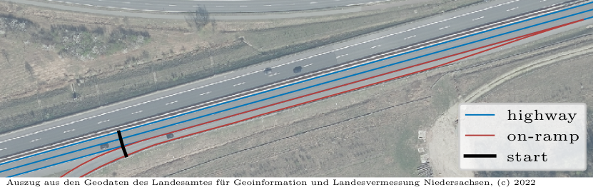
Figure 1: The on-ramp section near Cremlingen of the TFNDS. There are two mainline lanes denoted as highway and one acceleration lane denoted as on-ramp.

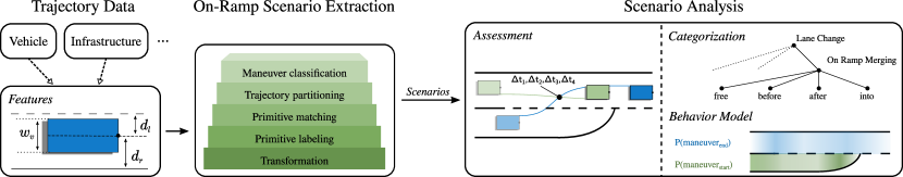
Figure 2: The proposed framework for on-ramp scenario extraction and analysis. The trajectory data can be supplied by various sources and just needs to be converted to provide the required Features which are used for scenario extraction. The scenarios are assessed, categorized and the on-ramp behavior is characterized in the Scenario Analysis module.

I-A Related work

The extraction of scenarios has been a broadly discussed topic in the research community for several years and has become even more relevant with the recent shift to a scenario-driven validation approach. A short overview of recent activities in this domain is given in the following.

Various approaches exist in literature to tackle the problem of scenario extraction in trajectory data. In general, the aim is to find certain characteristic time intervals in a multivariate time series. Supervised learning methods such as the Support Vector Machine (SVM) and Artificial Neuronal Network (ANN) were proposed by [11, 12, 13, 14]. However, the inherent drawback of these approaches is the training of (hyper) parameters based on ground truth data.

A comparative study for scenario extraction is conducted by Erdogan et al. [15] with a rule-based, supervised (Recurrent Neuronal Network (RNN)) and unsupervised learning ($k$-NN and DTW) method. Although the RNN is superior to the unsupervised learning method, it is more prone to sensor noise [15] which is inevitable in real-world data.

An alternative to supervised learning-based methods are approaches for clustering, i.e., unsupervised learning methods. Montanari et al. [16] slice time-series into chunks based on artificially created signals with empirically defined parameters and Agglomerative Hierarchical Clustering (AHC). The final interpretation of clusters is performed manually to find different variants of lane changes. This problem is inherent with non-deterministic unsupervised learning methods such as AHC, Random Forest Clustering [17] or HMM [18] and post-processing steps are required to recover the semantics either manually or automatically [19]. For instance, Elspas et al. [20] employ regular expressions to find maneuvers in the trajectory data after clustering it into symbolic states. However, they show that crafting the patterns has a significant impact on identification accuracy.

I-B Contribution

This work proposes a novel approach for extraction and analysis of on-ramp merging scenario from NTD contributing to setting up an extensive dataset of on-ramp merging scenarios for testing. Therefore, this work follows the divide and conquer strategy by decomposing an on-ramp maneuver into substates, the primitives. This abstract representation allows finding and classifying merging maneuvers robustly, as shown in a previous work [18] for lane-change maneuvers. An HMM is employed to represent the trajectory in the primitive domain, and DTW is used to compare the partitioned trajectory with patterns representing different variants of an on-ramp maneuver in the primitive domain.

The approach is applied to extract on-ramp scenarios from NTD of the TFNDS and analyze the on-ramp behavior of traffic participants. These insights are valuable especially in the context of mixed-traffic of CAV and traditional vehicles. Therefore, the SMoS PET is used for finding critical situations and to create a decision tree for categorizing merging scenarios according to the occupancy of the mainline.

I-C Paper structure

The remaining paper is structured as follows. In Section II, the proposed approach for on-ramp scenario extraction is presented. In Section III, the scenario analysis module is introduced, which allows categorizing and assessing the extracted scenarios. An evaluation of the scenario extraction method and an analysis of on-ramp merging scenarios follows in Section IV. Finally, the work concludes with a summary and outlook on future work in Section V.

II On-Ramp Merging Scenario Extraction

For the extraction and analysis of on-ramp merges in NTD provided by the TFNDS, this work proposes a methodology depicted in Fig. 2. In the following, the fundamental assumptions on on-ramp maneuvers are discussed, and the approach for on-ramp scenario extraction is presented.

II-A On-ramp merging maneuver

An on-ramp merging maneuver is a lane-change maneuver but in a different context. In fact, a road user performing an on-ramp maneuver is, in this work, assumed to drive on the acceleration lane of a highway’s on-ramp section and performs a lane-change to the left lane (see Fig. 1). A lane-change is in this work partitioned into multiple states, the driving primitives. This allows breaking down the complexity of a lane-change maneuver into more trivial driving actions which can be identified more easily. In addition, they are the building blocks for maneuver modelling and allow analyzing the behavior of traffic participants in the maneuver’s primitive domain space. [18]

From a lane-oriented point of view, the maneuver is divided into four distinct states (see Fig. 3). The vehicle is in the state Idle if it is in the middle of the lane. Moving towards the left lane marking, the vehicle enters the state Approach until it crosses it, where it changes to state Cross. The state Change denotes that the vehicle transitions to the target as long as the majority of the vehicle is on the source lane. Then, instead of changing to the state Depart, it will remain in the state Change but is associated to the target lane. Thus, the domain $D$ of driving primitives is $D=\{\text{{Idle}},\text{{Approach}},\text{{Cross}},\text{{Change}}\}$ for the lane-change or on-ramp maneuver. The aim is to, at first, transform the trajectory into the domain of driving primitives. By doing so, we can define different variants of a maneuver on the more abstract driving primitive domain level.

Figure 3: A lane-change is represented with four driving primitives [18]. From a lane-oriented point of view the state textitDepart is equal to Change but in the opposite direction.

Let us assume that the trajectory of a road user is transformed into the feature space depicted in Fig. 2. Hence, let $X=\mathbf{x}_{1},\mathbf{x}_{2},\dots,\mathbf{x}_{n}$ be the trajectory in the feature space so that $\mathbf{x}=[d_{l},d_{r},w]^{T}$ denotes the distance to the next left $d_{l}$ and next right $d_{r}$ marking, and $w$ the vehicle’s width. The aim is to find the most likely sequence $\mathcal{D}=\mathcal{D}_{1},\mathcal{D}_{2},\dots,\mathcal{D}_{n}$ with $\mathcal{D}$ as the primitive’s index in domain $D$, that represents the trajectory in the primitive domain defined by

$$\arg\max_{\mathcal{D}}\,P(\mathcal{D}\mid X)$$ (1)

with $P(\mathcal{D}\mid X)$ denoting the probability of observing the series of primitives $\mathcal{D}$ given a trajectory $X$. For solving (1), we use an HMM since it allows inferring a system’s hidden state based on its emitted information. In this particular case, the hidden states are the primitives and the information that the system emits is the trajectory. A HMM is defined as $\lambda=(\bm{A},\bm{B},\bm{\pi})$ with $\bm{A}$ as the state transition probabilities, $\bm{B}$ the matrix of observation probability conditioned on the current hidden state and $\bm{\pi}$ the initial state probabilities [21]. Since the observations are non-discrete we model each state’s emissions with a Gaussian Mixture Model (GMM). Assuming that $\lambda$ is a trained HMM with Gaussian emissions, the Viterbi algorithms can be utilized for solving the problem defined in (1) [22]. That is, finding the optimal sequence of primitives given the observations.

Note that the features depicted in Fig. 2 are not used directly, but a transformation is applied that allows supporting different vehicles and lanes. The features are the distance from the vehicle’s center to the lane’s center $d_{c}$ and a marker $\kappa$ indicating the vehicle is crossing a lane border. The HMM parameters used in this work are shown in TABLE I taken from a previous work [18]. The state transition matrix is denoted as Transition probability and the state emission via State distribution. Note that only the two adjacent primitives for each primitive have a significant transition likelihood which is coherent with our expectations and the states depicted in Fig. 3 since a vehicle should not switch between, e.g., the primitives Approach and Change and thus skipping Cross.

TABLE I: The HMM parameter used for finding the most likely sequence of lane-change primitives given a trajectory.

	Transition probability $\bm{A}$				State distribution $\bm{B}$
Primitive	Idle	Approach	Cross	Change	$d_{c}$	$\kappa$
Idle	$98.94$	$1.03$	$0.03$	$0.00$	$0.09\pm 0.06$	$0.00$
Approach	$1.46$	$97.53$	$1.01$	$0.00$	$0.33\pm 0.08$	$0.00$
Cross	$0.47$	$8.28$	$86.17$	$5.08$	$0.53\pm 0.09$	$1.00$
Change	$0.00$	$0.33$	$5.98$	$93.69$	$0.89\pm 0.11$	$1.00$

II-B Scenario extraction

A road user on the acceleration lane might change arbitrarily between the driving primitive states, and there could be multiple interesting situations to study. For instance, a driver on the acceleration lane could misjudge the velocity of a vehicle on the mainline and starts the merging maneuver. The driver reevaluates the situation during the maneuver and aborts it by changing back to the acceleration lane to prevent a critical situation. Consequently, not only the on-ramp maneuver is interesting, but also the canceled one. Due to that, we need to find the sequences within the trajectory representing these situations. If $\mathcal{D}=\mathcal{D}_{1},\mathcal{D}_{2},\dots,\mathcal{D}_{n}$ is the series of primitives, it will be divided into sequences $\mathcal{S}=\{\mathcal{S}_{1},\mathcal{S}_{2},\dots,\mathcal{S}_{k}\}$ with $k\ll n$ such that $\forall\mathcal{S}_{i}\in\mathcal{S}:\mathcal{S}_{i}^{k}\geq\xi$ with $\mathcal{S}_{i}^{k}$ as the $k^{th}$ primitive of the $i^{th}$ partition and $\xi$ defining the lower primitive bound. For instance, if $\xi=2$ a sequence represents a situation where a road user is either in the state Cross or changing between Cross and Change. In fact, the work uses $\xi=2$ for on-ramp maneuver extraction since the aim is to analyze the merging maneuver focussing on the interval where the vehicle transitions between the lanes.

For scenario identification, the sequences $\mathcal{S}=\mathcal{S}_{1},\mathcal{S}_{2},\dots$ need to be classified according to the relevant on-ramp variants. If $\mathcal{H}=\mathcal{H}_{0},\mathcal{H}_{1},\dots$ is the set of patterns representing the variants in the primitive domain, the aim is to find the most likely pattern $\widehat{\mathcal{H}}$ defined by

$$\widehat{\mathcal{H}}=\arg\max_{\mathcal{H}}\;d\left(\mathcal{S}_{i},\mathcal{H}\right)$$ (2)

with $d(\mathcal{S}_{i},\mathcal{H}_{j})$ denoting the similarity between both series. For time-series similarity estimation in (2), DTW is employed. For further details, the interested reader is referred to [18].

III Scenario categorization and assessment

The identified on-ramp merging scenarios using the approach presented in the previous section are processed in the Scenario Analysis component for situation assessment, scenario categorization and behavior modeling as depicted in Fig. 2. For the assessment of scenarios in terms of the criticality so called Surrogate Measures of Safety (SMoS) are typically utilized. For lane changes, the PET is broadly used [23, 9] for that purpose and thus chosen for this work since it allows assessing a certain situation but also provides information for further scenario categorization. In fact, this work will use a decision tree for scenario categorization based on the mainline’s occupancy and the PET.

III-A Situation assessment

The PET is the time difference between the first object leaving and the second object entering a conflict area [24]. In the following, the first is denoted as the ego vehicle and the latter as the challengers as defined in [25]. The lower the PET between two objects, the higher the potential criticality. This work assumes that the conflict area is defined by the four intersection points of the ego vehicle’s rear left and front left edges to the rear right and front ride edges of the challengers (see Fig. 2). Let $\mathcal{C}=\mathcal{C}_{1},\mathcal{C}_{2},\dots$ be the challengers on the mainline with $\mathcal{C}_{i}=\mathbf{c}_{1},\mathbf{c}_{2},\dots$ as the challenger’s trajectory that consists of the vehicle’s front right and rear right position. Furthermore, let $\mathcal{X}=\mathbf{x}_{1},\mathbf{x}_{2},\dots$ be the ego vehicle’s trajectory with its front left and rear left position. Then, $\mathcal{P}=\{\mathbf{p}_{1},\mathbf{p}_{2},\mathbf{p}_{3},\mathbf{p_{4}}\}$ are the four intersection points between a challengers and the ego vehicle’s trajectory. For PET estimation, the difference in time of arrival $T_{\mathcal{C}_{i}}=\{\Delta t_{1},\Delta t_{2},\Delta t_{3},\Delta t_{4}\}$ with $\Delta t=t_{ego}-t_{\mathcal{C}_{i}}$ and $t_{ego}$ of the ego vehicle’s and $t_{\mathcal{C}_{i}}$ the challenger’s arrival time at the intersection point $\mathbf{p}\in\mathcal{P}$ is calculated. Given the time-differences, the $\operatorname{PET}(\mathcal{C}_{i})$ between the ego vehicle and the candidate $\mathcal{C}_{i}$ is defined as

$$\operatorname{PET}(\mathcal{C}_{i})=\{\Delta t\mid\,\Delta t\in T_{\mathcal{C}_{i}}\wedge\lvert\Delta t\rvert=\min\lvert T_{\mathcal{C}_{i}}\rvert\}$$ (3)

with $\min\lvert T_{\mathcal{C}_{i}}\rvert$ the minimum absolute arrival time difference. The SMoS PET of on-ramp scenarios can be employed to find critical scenarios as exemplarily shown in Section IV.

III-B Scenario categorization

An on-ramp scenario can be further categorized according to the challengers [9]. In this work, only the challengers on the mainline are considered for categorization that are in the vicinity of the ego vehicle at that point in time where the ego vehicle performs a merging maneuver and is entering the primitive Cross. In particular, an on-ramp scenario is in this work specialized into four subtypes: free, in front, behind and into as depicted in Fig. 4.

Figure 4: On-ramp merging scenarios are specialized into four classes according to the position of challengers

For this categorization, a decision tree is created based on the presence of challengers on the mainline and the PET between the ego vehicle and all challengers of a scenario. The PET is used since the sign of the PET denotes the order of entering and leaving the conflict zone. The PET defined in (3) is positive if the ego vehicles arrives the intersection point after the challenger and negative vice versa. Hence, a scenario is classified as behind or in front if there is only one challenger $|\mathcal{C}|=1$ and $\operatorname{PET}(\mathcal{C}_{1})>0$ or $\operatorname{PET}(\mathcal{C}_{1})<0$ respectively. If there are at least two challengers $|\mathcal{C}|>2$ and $\exists\mathcal{C}_{i}\in\mathcal{C}:\operatorname{PET}(\mathcal{C}_{i})>0\wedge\mathcal{C}_{i}\in\mathcal{C}:\operatorname{PET}(\mathcal{C}_{i})<0$ the lane-change is classified as into. If there is no challenger on the mainline, the lane-change is classified as free. Note that this work assumes that there is no collision between challengers and the ego vehicle.

III-C Driver behavior model

The identification of on-ramp merging scenarios enables to derive behavioral models of the drivers, which can be employed to generate trajectories for more extensive simulation-based testing, e.g., in Carla [26] or SUMO [27]. This is especially of interest in the context of mixed traffic of CAV and traditional vehicles since CAV have to predict the behavior in this situations.

In this work, the focus is on the distribution of the merging maneuver’s start and end position as a simple use-case to demonstrate the potential of collecting scenarios with the proposed approach. For that purpose, let the merging-maneuver $m=(p_{1},p_{2})$ be defined by its start $p_{1}$ and end position $p_{2}$. However, instead of using the locations in a Cartesian Coordinate system, the positions are converted into the Frenét reference frame defined by the left lane border of the acceleration lane depicted in Fig. 5.

Figure 5: The trajectory in Frenét reference frame defined by the left border $r$ of the acceleration lane.

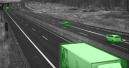
Figure 6: Images of the on-ramp section near Cremlingen of the TFNDS with overlayed bounding boxes. The dataset used in this work is collected in that area for scenario extraction and analysis.

This is an established method for, e.g., trajectory planning since it allows defining a trajectory relative to the road [28]. That is, the location $\mathbf{x}_{t}$ at time $t$ represented in a Cartesian Coordinate system is converted into a dynamic reference frame specified by the lane boundary’s representation $r$ according to [28] by

$$\mathbf{x}_{t}=f\left(\mathbf{x}_{t},r\right)+g\left(\mathbf{x}_{t},r\right)$$ (4)

with $f\left(\mathbf{x}_{t},r\right)$ denoting the distance of the position $\mathbf{x}_{t}$ on the lane $r$ and $g\left(\mathbf{x}_{t},r\right)$ the perpendicular distance between $\mathbf{x}_{t}$ and its projected sibling on the lane. Since only the relative position on the lane is relevant to describe the maneuver start and end position, the second component of (4) is neglected. Furthermore, since merging maneuvers can only occur when the acceleration lane meets the mainline, the start of the lane is defined at the point where the acceleration lane’s left lane border joins with the rightmost border of the highway lanes as denoted as the start line in Fig. 1. Hence, the maneuver start and end position is given by

$$m=\left(\frac{1}{\lvert r\rvert}f(\mathbf{x}_{t_{1}},r)-\nu,\frac{1}{\lvert r\rvert}f(\mathbf{x}_{t_{2}},r)-\nu\right)$$ (5)

with $\mathbf{x}_{t_{1}},\mathbf{x}_{t_{2}}$ as the road user’s location at the maneuver start and end respectively, $\nu$ the start position on the lane and $\lvert r\rvert$ the lane’s length from the start point. The latter is employed for position normalization to ensure that the results are independent of the acceleration lane length. The maneuver’s start and end positions defined in (5) is used in Section IV for further analysis.

IV Experiments

The following section evaluates the proposed approach for on-ramp merging extraction with a dataset of the TFNDS. The extracted scenarios are the basis for further analysis.

IV-A Dataset

The trajectory data used for the evaluation and analysis is collected at the on-ramp region at Cremlingen near Braunschweig in Germany, which is part of the TFNDS (see Fig. 1). The region is covered by four camera masts equipped with two stereo cameras. In Fig. 6 a sample image per camera is shown; row-wise from the top left to the bottom right. Only the stereo camera pair pointing to the on-ramp is shown for the first and last camera mast. The trajectory data was collected on three different days and various daytimes. Note that the used sampling strategy was to collect snippets of $90$ seconds each $300$ seconds. Due to this, only trajectories are considered in the analysis having a length greater than half of the on-ramp lane’s length to remove clipped trajectories.

The road association of a traffic participant was estimated for qualitative analysis of the proposed extraction method. Therefore, it is assumed that a trajectory performs a merging maneuver if the trajectory starts on the acceleration but ends on any highway lane. In all other cases, the traffic participant is associated with the highway. After filtering, the total number of trajectories in the dataset is $2465$ with $2321$ objects associated with the highway lanes and $144$ the on-ramp lane (performing a merging maneuver). The distribution of the observed objects on an hourly basis is depicted in Fig. 7.

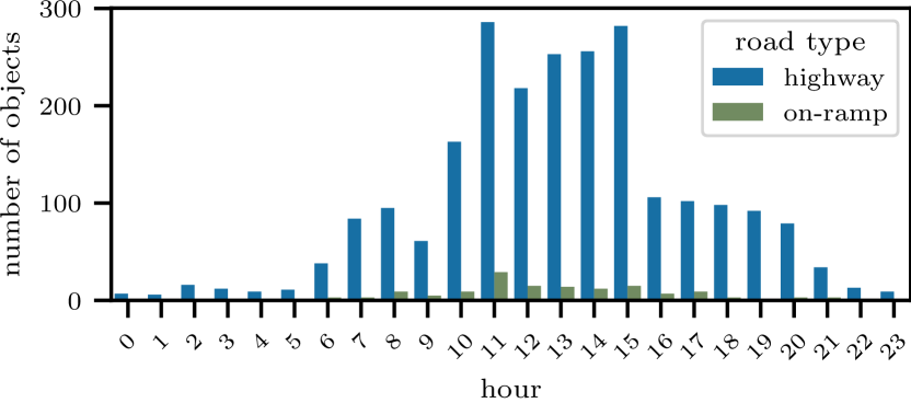
Figure 7: Distribution of the observed objects per road type on a hourly basis in the used dataset.

IV-B Scenario extraction evaluation

To evaluate the scenario extraction accuracy, the dataset is processed with the presented approach. Therefore, only objects driving on the on-ramp are considered. As a result, the approach correctly extracts $137$ of the $144$ merging scenarios and thus achieves an accuracy of $95.14\%$.

It turns out that the approach fails in lane-change identification if a lane-change starts at the end of the on-ramp lane so that the object crosses both lane marking. This is depicted in Fig. 8 showing the relation between the start and end positions of all maneuvers. Note that all positions in Fig. 8 are relative to the start of the lane as defined in Section III-C.

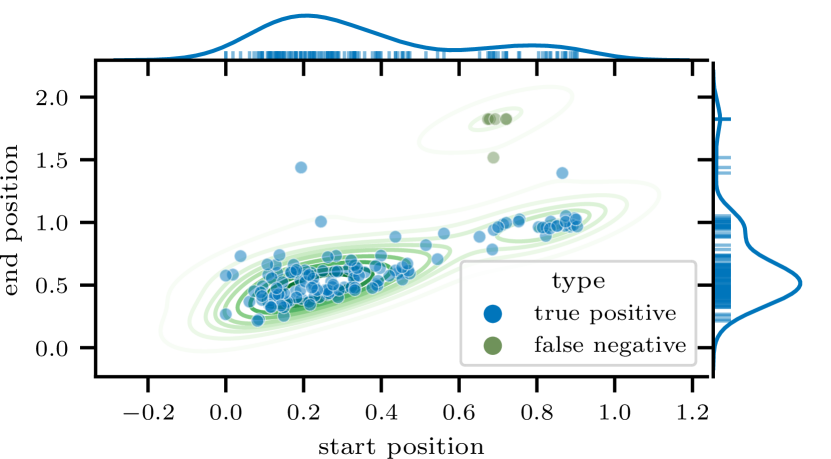
Figure 8: Overview of the correctly ($\bullet$) and incorrectly ($\star$) identified on-ramp merges start and end positions with object classes (color-encoded).

It is evident from Fig. 8 that the difference between correctly and incorrectly identified maneuvers is the end position. That is, maneuvers starting at the end of the on-ramp lane with a start position greater than $0.6$ and ending beyond it with an end position greater $1.4$ are not identified.

Overall, although the approach failed to extract all scenarios, the performance is appropriate for the use-case at hand since no false positives exist. This is because the TFNDS is collecting a vast amount of data, and missing scenarios is not critical but extracting misclassified scenarios is. The latter is due to the required resources for scenario extracting and saving. Moreover, those misclassified scenarios need to be identified and removed before further analysis. Otherwise, wrong conclusions about the on-ramp merging behavior could be drawn.

IV-C Merging behavior analysis

The representation of on-ramp maneuvers with the starting and end position allows analyzing the merging behavior. As depicted in Fig. 8, the distribution of start positions is bimodal with the majority of maneuver starting at the first half of the acceleration lane. This is also clearly visible in Fig. 9 depicting the start and end position’s cumulative distribution function (cdf) of all correctly extracted maneuvers. That is, $25\%$ of all maneuvers have a start position smaller than $0.16$ and $50\%$ smaller than $0.27$. Hence, most maneuvers start within the first half of the acceleration lane. In fact, $79.56\%$ of all maneuvers have a start position smaller than $0.5$ and $86.13\%$ start within the first three quarters. The opposite is the case for the maneuver end positions with $1.46\%$ within the first quarter and $39.42\%$ in the first half. The most traffic participants finish the on-ramp maneuver within the second half ($53.28\%$) and almost all ($92.70\%$) within the course of the acceleration lane. Hence, $7.30\%$ are still conducting the maneuver although the acceleration lane has already merged.

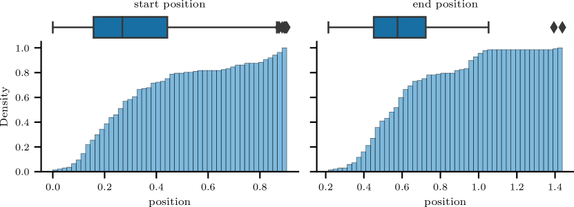
Figure 9: The cdf of maneuver start and end positions relative to the start and normalized w.r.t the length of the acceleration lane. Only the correctly extracted maneuvers are considered.

IV-D Scenario assessment

The Assessment module depicted in Fig. 2 uses the PET to relate the ego-vehicle on the on-ramp lane to challengers on the target lane. This enables to, for instance, find critical scenarios, i.e., scenarios with a low PET between the ego-vehicle and a challenger.

The PET distribution for the scenario categories behind, in front and into is depicted in Fig. 10. Note that the category free is missing since there is no challenger on the mainline. For the category into the sum of PETs values is used to represent each scenario with a single value which is related to the SMoS accepted gap time.

Fig. 10 shows that vehicles tend to merge onto the mainline quite close behind another vehicle with $50\%$ having a PET lower than $4.0$ seconds and $25\%$ lower than $2.6$ seconds. For the into type the PET is uniformly distributed within $[5.0;15.1]$ seconds and a mean of $9.7\pm 2.9$ seconds. The gap between a vehicle merging in front of another vehicle is even closer than for the behind class with $50\%$ having a PET lower than $3.0$ seconds and $25\%$ lower than $2.0$ seconds. Noteworthy is the situation with a PET of $0.08$ seconds and thus denotes a near-crash situation. This situation is depicted in Fig. 11 where the ego vehicle starts the lane-change maneuver and one second later (in transparent). In that scenario, a vehicle (in blue) merges onto the mainline which is occupied by a truck (in green). Although the PET indicates that the scenario is critical, Fig. 11 shows that the situation becomes uncritical since the gap between both vehicles increases.

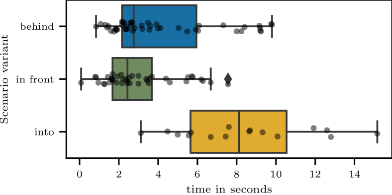
Figure 10: Distribution of the PET time for all identified on-ramp scenarios of type behind and in front and the accepted gap time for into.

V Conclusion

A scenario-based validation approach for CAV demands information from real-world driving as provided by the TFNDS. However, a challenge is to annotate the data with the scenarios of interest.

This work addresses this issue and proposes a novel methodology for on-ramp scenario extraction and analysis. The extracted scenarios are categorized and assessed using the PET which also enables the identification of critical scenarios. Evaluations have shown that the approach robustly extracts scenarios with an accuracy of $95.14\%$. However, the results also indicate that the method fails identifying maneuvers starting at the merging lane’s end. This will be the subject of future works.

Furthermore, the maneuver behavior in terms of the start and end position is analyzed. The first results indicate that most vehicles tend to merge on the mainline at the first half of the acceleration line. In follow-up works, a more comprehensive dataset will be employed to analyze further the behavior of the ego vehicle and challengers in on-ramp merging scenarios.

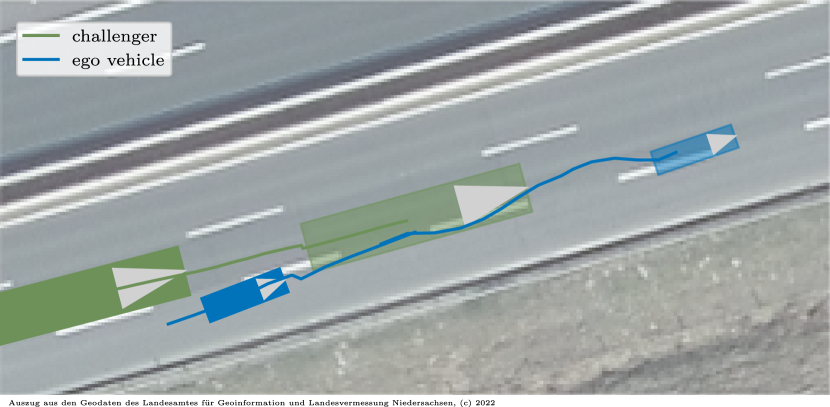
Figure 11: The identified critical on-ramp scenario at the start of the lane change maneuver and one second later (with higher transparency).

References

- [1] J. Günther, H. Lehmann, P. Nuss, and K. Purr, Resource-efficient Pathways Towards Greenhouse-gas-neutrality-RESCUE: Summary Report. Umweltbundesamt, 2019.
- [2] P. Kopelias, E. Demiridi, K. Vogiatzis, A. Skabardonis, and V. Zafiropoulou, “Connected & autonomous vehicles – Environmental impacts – A review,” Science of The Total Environment, vol. 712, p. 135237, 2020.
- [3] A. Papadoulis, M. Quddus, and M. Imprialou, “Evaluating the safety impact of connected and autonomous vehicles on motorways,” Accident Analysis & Prevention, vol. 124, pp. 12–22, 2019.
- [4] T. Guan and C. W. Frey, “Predictive energy efficiency optimization of an electric vehicle using traffic light sequence information*,” in 2016 IEEE International Conference on Vehicular Electronics and Safety (ICVES), 2016, pp. 1–6.
- [5] H. Winner, K. Lemmer, T. Form, and J. Mazzega, PEGASUS—First Steps for the Safe Introduction of Automated Driving. Switzerland: Springer International Publishing, 2018, ch. Vehicle Systems and Technologies Development, pp. 185–195.
- [6] S. Hallerbach, Y. Xia, U. Eberle, and F. Köster, “Simulation-based identification of critical scenarios for cooperative and automated vehicles,” SAE Intl. J CAV, vol. 1, pp. 93–106, 04 2018.
- [7] C. Neurohr, L. Westhofen, M. Butz, M. H. Bollmann, U. Eberle, and R. Galbas, “Criticality analysis for the verification and validation of automated vehicles,” IEEE Access, vol. 9, pp. 18 016–18 041, 2021.
- [8] W. Damm, E. Möhlmann, T. Peikenkamp, and A. Rakow, “A formal semantics for traffic sequence charts,” in Principles of Modeling. Springer, 2018, pp. 182–205.
- [9] W. Qi, W. Wang, B. Shen, and J. Wu, “A modified post encroachment time model of urban road merging area based on lane-change characteristics,” IEEE Access, vol. 8, pp. 72 835–72 846, 2020.
- [10] H. Elrofai, J. Paardekooper, E. d. Gelder, S. Kalisvaart, and O. Op den Camp, “Streetwise: scenario-based safety validation of connected automated driving,” 2018.
- [11] P. Kumar, M. Perrollaz, S. Lefèvre, and C. Laugier, “Learning-based approach for online lane change intention prediction,” in 2013 IEEE Intelligent Vehicles Symposium (IV), 2013, pp. 797–802.
- [12] R. Izquierdo, I. Parra, J. Muñoz-Bulnes, D. Fernández-Llorca, and M. A. Sotelo, “Vehicle trajectory and lane change prediction using ANN and SVM classifiers,” in 2017 IEEE 20th International Conference on Intelligent Transportation Systems (ITSC), 2017, pp. 1–6.
- [13] S. Ramyar, A. Homaifar, A. Karimoddini, and E. Tunstel, “Identification of anomalies in lane change behavior using one-class SVM,” in 2016 IEEE International Conference on Systems, Man, and Cybernetics (SMC), Oct 2016, pp. 004 405–004 410.
- [14] N. Monot, X. Moreau, A. Benine-Neto, A. Rizzo, and F. Aioun, “Comparison of rule-based and machine learning methods for lane change detection,” in 2018 21st International Conference on Intelligent Transportation Systems (ITSC), Nov 2018, pp. 198–203.
- [15] A. Erdogan, B. Ugranli, E. Adali, A. Sentas, E. Mungan, E. Kaplan, and A. Leitner, “Real-World Maneuver Extraction for Autonomous Vehicle Validation: A Comparative Study,” in 2019 IEEE Intelligent Vehicles Symposium (IV), June 2019, pp. 267–272.
- [16] F. Montanari, R. German, and A. Djanatliev, “Pattern recognition for driving scenario detection in real driving data,” in 2020 IEEE Intelligent Vehicles Symposium (IV), 2020, pp. 590–597.
- [17] F. Kruber, J. Wurst, and M. Botsch, “An Unsupervised Random Forest Clustering Technique for Automatic Traffic Scenario Categorization,” in 2018 21st International Conference on Intelligent Transportation Systems (ITSC), Nov 2018, pp. 2811–2818.
- [18] L. Klitzke, C. Koch, and F. Köster, “Identification of Lane-Change Maneuvers in Real-World Drivings With Hidden Markov Model and Dynamic Time Warping,” in 2020 IEEE 23rd International Conference on Intelligent Transportation Systems (ITSC), 2020, pp. 1–7.
- [19] W. Wang, J. Xi, and D. Zhao, “Driving Style Analysis Using Primitive Driving Patterns With Bayesian Nonparametric Approaches,” IEEE Transactions on Intelligent Transportation Systems, vol. 20, no. 8, pp. 2986–2998, Aug 2019.
- [20] P. Elspas, J. Langner, M. Aydinbas, J. Bach, and E. Sax, “Leveraging regular expressions for flexible scenario detection in recorded driving data,” in 2020 IEEE International Symposium on Systems Engineering (ISSE), 2020, pp. 1–8.
- [21] L. Rabiner, “A tutorial on hidden markov models and selected applications in speech recognition,” Proceedings of the IEEE, vol. 77, no. 2, pp. 257–286, 1989.
- [22] J. A. Bilmes et al., “A gentle tutorial of the EM algorithm and its application to parameter estimation for Gaussian mixture and hidden Markov models,” International Computer Science Institute, vol. 4, no. 510, p. 126, 1998.
- [23] H. Behbahani and N. Nadimi, “A framework for applying surrogate safety measures for sideswipe conflicts,” International Journal for Traffic & Transport Engineering, vol. 5, no. 4, pp. 371–383, 2015.
- [24] D. Gettman and L. Head, “Surrogate safety measures from traffic simulation models,” Transportation Research Record, vol. 1840, no. 1, pp. 104–115, 2003.
- [25] H. Weber, J. Bock, J. Klimke, C. Roesener, J. Hiller, R. Krajewski, A. Zlocki, and L. Eckstein, “A framework for definition of logical scenarios for safety assurance of automated driving,” Traffic Injury Prevention, vol. 20, no. sup1, pp. S65–S70, 2019.
- [26] A. Dosovitskiy, G. Ros, F. Codevilla, A. Lopez, and V. Koltun, “CARLA: An open urban driving simulator,” in Proceedings of the 1st Annual Conference on Robot Learning, ser. Proceedings of Machine Learning Research, S. Levine, V. Vanhoucke, and K. Goldberg, Eds., vol. 78. PMLR, 13–15 Nov 2017, pp. 1–16.
- [27] M. Behrisch, L. Bieker, J. Erdmann, and D. Krajzewicz, “SUMO – Simulation of Urban MObility: An Overview,” in SIMUL 2011, S. . U. of Oslo Aida Omerovic, R. I. R. T. P. D. A. Simoni, and R. I. R. T. P. G. Bobashev, Eds. ThinkMind, Oktober 2011.
- [28] M. Werling, J. Ziegler, S. Kammel, and S. Thrun, “Optimal trajectory generation for dynamic street scenarios in a frenét frame,” in 2010 IEEE International Conference on Robotics and Automation, 2010, pp. 987–993.