Number-phase uncertainty relations and bipartite entanglement detection in spin ensembles
Abstract
We present a method to detect bipartite entanglement based on number-phase-like uncertainty relations in split spin ensembles. First, we derive an uncertainty relation that plays the role of a number-phase uncertainty for spin systems. It is important that the relation is given with well-defined and easily measurable quantities, and that it does not need assuming infinite dimensional systems. Based on this uncertainty relation, we show how to detect bipartite entanglement in an unpolarized Dicke state of many spin- particles. The particles are split into two subensembles, then collective angular momentum measurements are carried out locally on the two parts. First, we present a bipartite Einstein-Podolsky-Rosen (EPR) steering criterion. Then, we present an entanglement condition that can detect bipartite entanglement in such systems. We demonstrate the utility of the criteria by applying them to a recent experiment given in K. Lange et al. [Science 360, 416 (2018)] realizing a Dicke state in a Bose-Einstein condensate of cold atoms, in which the two subensembles were spatially separated from each other. Our methods also work well if split spin-squeezed states are considered. We show in a comprehensive way how to handle experimental imperfections, such as the nonzero particle number variance including the partition noise, and the fact that, while ideally BECs occupy a single spatial mode, in practice the population of other spatial modes cannot be fully suppressed.
1 Introduction
Entanglement lies at the heart of many problems in quantum mechanics and has attracted an increasing attention in recent years [1, 2, 3, 4]. Entangled states can be used for metrology in order to obtain a sensitivity higher than the shot-noise limit [5, 6, 7] and can also be used as a resource for certain quantum information processing tasks [8, 9, 10, 11, 12]. Entanglement also plays an important role in quantum computing making it possible that quantum computers outperform their classical counterparts for several problems such as prime factoring or searching [13, 14]. Moreover, experiments realizing macroscopic quantum entanglement might give answers to fundamental questions in quantum physics [15, 16].
When in an experiment entanglement is created, it is important to detect it. Thus, in many quantum physics experiments the creation of an entangled state is followed by measurements. Based on the results of these measurements, the experimenters conclude that the produced state was entangled. However, in many-particle experiments the possibilities for quantum control are very limited. In particular, the particles cannot be individually addressed. In such systems, the entanglement can be created and detected with collective operations. The first entanglement criterion based on such collective quantities was the spin-squeezing criterion that detects entanglement in an ensemble of spin- particles, and it detects entangled states that are close to be fully polarized [17], even multipartite entanglement can be detected in such states [17]. Later, a full set of generalized spin-squeezing criteria have also been defined [18, 19]. Such criteria can detect states very different from usual spin-squeezed states. For instance, unlike spin-squeezed states, unpolarized symmetric Dicke states have a zero expectation value for all spin components and the precision in parameter estimation in linear interferometers using such states can reach, in principle, the maximal Heisenberg-scaling with the number of particles [20, 21, 22]. Even criteria for multiparticle entanglement have been developed for Dicke states [23, 24, 25] and there are criteria that detect metrologically useful entanglement [26, 27, 28]. Moreover, criteria for an ensemble of particles with a spin larger than have also been found [29, 30, 31, 32].
The entanglement criteria mentioned above have been tested in a variety of physical systems [33, 21, 22]. In photonic systems, symmetric Dicke states have been created [34, 35, 36, 37, 38]. In cold trapped ions, spin-squeezed states [39], W-states, i.e., Dicke states with a single excitation [40] have been realized and there is a general scheme for obtaining various kind of Dicke states [41]. In atomic ensembles, spin-squeezed states [42, 43, 44, 45, 46, 47] and many-body singlet states have been realized [48, 49]. Large scale quantum entanglement has also been created in Bose-Einstein Condensates (BEC). Spin-squeezed states of two-state atoms have been realized in several experiments [42, 50, 51, 52, 53, 54, 22]. Multipartite entanglement has been detected in these states, and it has also been demonstrated that such states are useful for quantum metrology.
From the point of view of our paper it is very relevant that, recently, symmetric Dicke states have also been created in BECs [20, 55]. Apart from entanglement, even metrological usefulness of Dicke states has been verified [20, 27]. A Dicke state of around 8000 particles has been realized and multipartite entanglement up to particles has been detected within an error of two standard deviations [24, 25]. Moreover, Dicke states of more than 10000 spin-1 atoms and 630-particle entanglement has been detected within an error of a single standard deviation [56].
As a natural next step, it is important to detect entanglement between two parts of such collective spin states, since bipartite entanglement between spatially separated subsystems is the type of entanglement most useful for quantum information processing applications. It has been shown that multipartite entanglement of bosonic two-state atoms can be converted into bipartite entanglement by splitting the ensemble into two [57]. However, can this powerful theoretical result be verified in an experiment, where noise and other imperfections are present? The question is even more timely since the detection of bipartite entanglement of high-dimensional systems raised a lot of attention [58, 59]. In a recent experiment, bipartite entanglement was successfully detected in a Dicke state created with thousands of atoms and distributed into two spatially separated regions [60].
Another form of quantum correlations, stronger than entanglement, termed Einstein-Podolsky-Rosen (EPR) steering [61, 62, 63, 64, 65], has also been recently detected in photonic systems [66], as well as in BECs [67]. Methods to detect EPR correlations in spatially separated parties, i.e., in a two-well BECs have also been studied theoretically [68, 69, 70]. Experimentally, the observation of EPR correlations between spatially separated modes was achieved in split-squeezed atomic ensembles [71], while entanglement has also been detected using a criterion developed by Giovannetti et al. in Ref. [72]. EPR correlations have also been detected with spin-nematic squeezing [73].
All entanglement conditions employed in the recent experiments mentioned above are based on variances of collective spin components, and it was recently observed how such criteria can be converted into lower bounds to entanglement monotones, thus allowing for the quantification of entanglement with the same information [74]. Thus, finding efficient entanglement witnesses is very relevant also for the quantification of entanglement.
In this paper, we present entanglement criteria that verify the presence of bipartite entanglement between spatially separated parts of a condensate. We also introduce an EPR steering criterion. Our criteria are particularly well suited for symmetric unpolarized Dicke states given as
| (1) |
where and are the basis states of a two-level atom, and is even and the summation is over all distinct permutations of the particles. We will call simply Dicke state in the following. For an equal partitioning of the particles, the entanglement of formation of is large, which will be discussed in Appendix A. This gives us a further strong motivation to try to detect bipartite entanglement in these states [75]. Our methods also work for other quantum states, such as spin-squeezed states.
We obtain criteria that detect entanglement and EPR steering between two parts of the Dicke state in Eq. (1). For that, we divide the system into two subsystems, which we denote by “” and “” The particle number operators in the two subsystems fulfill
| (2) |
In practice, this means that an atomic cloud is spatially separated into two regions as in Fig. 1. At this point we have to stress an important property of real experiments. The total particle number fluctuates from experiment to experiment. Moreover, even if the total particle number remained fixed, the particle numbers and will change from experiment to experiment due to fundamental quantum effects that we will discuss later. Thus, the quantum states do not live in a single Hilbert space with a fixed and but rather they live in several such Hilbert spaces. A general state of our system can be written as [76, 77]
| (3) |
where have definite particle numbers in the two subsystems, and are probabilities. Here, the local total angular momentum depends on the local particle number via the relation for
Note that here we are discarding superpositions between states with different number of particles within subsystems and The operators appearing in our entanglement criteria conserve the particle number within the subsystems, thus they cannot distinguish superpositions of states with different particle numbers from a mixture of such states. In any case, even if the state of the system had a superposition of states with different subsystem particle numbers, we can remove them with the projection
| (4) |
where is the state of the system and projects to a subspace with fixed particle numbers [77, 78]. Since our criteria cannot distinguish from in Eq. (3), we will consider states of the form given in Eq. (3). This is also the relevant case in experiments, where the measurement will always project onto a state with a definite particle number.
Our criteria are formulated with the moments of the collective angular momentum coordinates. For a state with a given and they are defined as
| (5) |
where and denotes a component of the spin. Analogously, we can define and for the two subsystems. Naturally, the angular momentum components fulfill
| (6) |
.
For states given in Eq. (3), we compute expectation values of observables as follows. Let us consider an operator
| (7) |
where we used the notation “” stressing that are the total angular momentum operators, and are defined as and where and are particle number operators. For simplicity, we will omit “” in the future. It will be clear from the context, when we talk about operators. Moreover, denotes a two-variable function and is an operator constructed as a function of angular momentum components and Then, the expectation value of can be obtained as
| (8) |
For subsystem , a formalism similar to that of Eq. (3) can be used
| (9) |
where have definite particle numbers. The expectation value of an operator can be computed analogously to Eq. (8). Analogous statements hold for subsystem
In this paper, we will present criteria that are satisfied by a local hidden state model. A local hidden state model means the following. There is a hidden variable with a probability distribution given by For each value of the hidden variable there is a (hidden) state of subsystem described by the normalized density matrix Any expectation value of an operator acting on can be obtained as a weighted average of expectation values for a given
| (10) |
Subsystem on the other hand, is described differently. The local hidden state model provides for each and operator acting on subsystem a distribution where are the outcomes of measuring If the correlations cannot be described by such a local hidden state model, then is called steerable. We will give a more complete description in the main text.
We will also present criteria to detect entanglement in the system. The state given in Eq. (3) is separable if and only if all are separable, i.e., they are mixtures of product states [77] and can be written as
| (11) |
where and are states of the subsystems and , respectively. If a quantum state cannot be decomposed as in Eq. (11), then it is entangled and the mixture of such states as in Eq. (3) is also entangled.
We will now present the three inequalities that will be proven in Sec. 2. First, we present the basis of our work, an uncertainty relation that can be considered a number-phase uncertainty for atomic ensembles. Unlike in the case of bosonic modes, now we do not assume infinite systems. It is also important that our relation is given in terms of well defined and easily accessible quantities.
Observation 1. For any quantum state, the following uncertainty relation
| (12) |
holds for Here, we formulated the uncertainty relation for one of the two subsytems.
Based on this, we find the following EPR steering condition. Essentially, a local hidden state model means the following. Subsystem is described by a density matrix conditioned on measurements on subsystem Thus, criteria satisfied by states with a local hidden state model are uncertainty relations for subsystem conditioned on measurements on subsystem
Observation 2. All quantum states that admit a local hidden state model must satisfy
| (13) |
Here, the inference variance is the variance of estimating based on measurement results on subsystem for quantum states with a local hidden state model. Note that it can be smaller than When the criterion is applied to an experiment, one considers the substitution
| (14) |
where the estimates are given as
| (15) |
for with constants111Instead of Eqs. (14) and (15), typically they write [62, 63, 64, 65] (16) where is a real number. We have to choose such that the variance is minimal. This is the case if With that choice, holds, and we arrive at Eq. (14).. Any quantum state that violates Eq. (13) is steerable. The inequality in Eq. (13) holds for all non-steerable states, and for any choice of the real parameters Therefore, the latter can be optimized in such a way that the violation is maximized, i.e., the left-hand side of Eq. (13) is minimized. Later, we will show that for an ideal Dicke state of many particles, the optimal choice for is
| (17) |
Then, we present a criterion detecting entanglement.
Observation 3. For separable states in bipartite systems
| (18) |
holds, where we define the difference between the angular momentum components in the two parts as
| (19) |
for
If we set the according to Eq. (17) then the left-hand side of Eq. (13) is identical to the left-hand side of Eq. (18). Let us compare the right-hand sides. For states living in the symmetric (i.e., bosonic) subspace such that as we will see later, the right-hand side of Eq. (13) is around 4 times smaller than that of Eq. (18). Thus, for such states, it is more difficult to violate the EPR steering criterion (13) than the entanglement criterion (18), which is consistent with the fact that steering is typically harder to get than entanglement.
In this paper, we will prove the relations mentioned above and show that these relations detect entanglement in a condensate split into two parts. Our method will handle the problem of fluctuating particle numbers, which has two different manifestations. On the one hand, the total particle number varies from experiment to experiment. On the other hand, when the ensemble is split, the particle number in the two subensembles will not be exactly half of the total particle number. Both of these effects make the detection of entanglement more difficult, since they decrease the violation of the entanglement criteria. An appropriate normalization of the measured quantities can reduce the problem mentioned above. We show this in detail for the case of the splitting noise, which we call partition noise.
Our method can also tolerate another imperfection appearing in experiments. While ideally BECs occupy a single spatial mode, in practice the population of other spatial modes cannot be fully suppressed. This is partly due to the fact that BECs are prepared experimentally at some nonzero temperature. Hence, a quantum state realized with a BEC of two-level atoms will never be in a perfectly symmetric state [77]. Due to the complexity of the appropriate modelling, such effects have not been considered in many cases when the state of the ensemble was obtained via tomography, and in some cases they were taken into account through ad-hoc methods. We work out criteria that are valid also for states that are not perfectly symmetric.
Our paper is organized as follows. In Sec. 2, we prove the uncertainty relation (12). We also prove the EPR steering criterion (13) and the entanglement criterion (18). In Sec. 3, we calculate relevant quantities for the split Dicke state and present other versions of our criteria with a normalization that handles the partition noise in Dicke states, i.e., the fluctuation of the particle numbers in the two halves of the system due to splitting. In Sec. 4, we apply our criteria to various ideal quantum states as well as to an experiment in which a Dicke state has been prepared. Furthermore, we also test our criteria numerically on split spin-squeezed states.
2 Derivation of the inequalities
In this section, we prove the number-phase-like uncertainty relation given in Observation 1. Then, we prove the EPR relation given in Observation 2 and the entanglement criterion in Observation 3.
2.1 Number-phase-like uncertainty
Here, we derive an uncertainty relation that resembles a number-phase complementarity relation.
Proof of Observation 1. Let us first prove that the usual Heisenberg uncertainty relation for some and operators
| (20) |
with is valid for a fluctuating number of particles and we formulated the uncertainty for one of the subsystems Let us consider the following series of inequalities
| (21) | |||||
where again The first inequality in Eq. (21) is due to the concavity of the variance. The second inequality holds because Eq. (20) is valid for a state with fixed It is also due to the relation (see, e.g., Ref. [79])
| (22) |
where which can be obtained straightforwardly from the Cauchy-Schwarz inequality222The Cauchy-Schwarz inequality is Equation (22) can be proved taking and . The last inequality in Eq. (21) is due to the basic properties of the absolute value. With that we proved that the Heisenberg uncertainty relation is true for states with a varying particle number. Note that our proof is valid even if and depend on .
Now we consider the Heisenberg uncertainty relations
| (23) |
By summing the two inequalities we obtain
| (24) |
Then, by adding to both sides, and dividing by we arrive at the uncertainty relation Eq. (12).
Equation (12) is similar to a number-phase uncertainty relation [60]. In Eq. (12), the first term represents the fluctuations in the particle number difference and the second term represents the fluctuations in the phase difference. In Appendix B, we show how Eq. (12) can be connected to the literature on number-phase uncertainties.
It is interesting to note that the term with in Eq. (12) has a constant part. The well-known Heisenberg uncertainty with the canonical and operators does not have such a constant. For that uncertainty, when is approaching zero, is approaching infinity. In our case, the uncertainties of the angular momentum components are bounded from above for a given particle number. Thus, such a constant added to is needed to obtain a meaningful uncertainty relation with angular momentum components. If is zero and there were not a constant included in the first term, then an uncertainty could be satisfied only if the right-hand side of the inequality were zero, or the second term on the left-hand side were infinite, which is impossible. Due to the constant term, a state fully polarized in the -direction, having saturates the relation given in Eq. (12) with a nonzero value on the right-hand side.
2.2 Einstein-Podolsky-Rosen criterion
Here, we prove the criterion for steering given in Eq. (13). An important EPR condition with collective spin operators is given as [80, 81, 82]
| (25) |
where the right-hand side can be improved considering an inferred value based on measurements on party [65]. These relations are tailored for states that have a spin almost fully polarized in the -direction. To construct a similar criterion that is also suitable to detect unpolarized states, such as the state given in Eq. (1), we can use directly Eq. (12)333Note that there is a relation stronger than Eq. (25), where there is an inferred quantity also on the right-hand side. It can detect also unpolarized states [80, 81, 82]..
Proof of Observation 2. We build on the explanation of local hidden state models given in the introduction and the relation given in Eq. (10). Given that one measures an observable on subsystem and gets outcome , one can associate to subsystem a positive matrix (i.e., a quantum state that is not normalized)
| (26) |
After all outcomes are sampled, the whole ensemble of such positive matrices (termed assemblage) satisfies where is the reduced density matrix of . This is consistent with the fact that and initially shared a common quantum state .
Now we will derive relations that are valid for states with a local hidden state model. They are uncertainty relations for subsystem conditioned on measurements on subsystem Given the measurement outcomes on , one can try to build estimates for all operators The estimate is typically a function of the measurement outcomes on subsystem
| (27) |
where we define the normalized density matrix
| (28) |
It is easy to see that the best estimate we obtain for
| (29) |
In this case, we obtain
| (30) |
Due to the concavity of the variance and based on Eq. (28), we can write that
| (31) |
Based on Eq. (30) and Eq. (31), for such a local hidden state model the inference variance is lower bounded as [62, 63, 64, 65]
| (32) |
On the right-hand side there is the estimation precision reached when we know the local hidden variable. The inference variance cannot be lower than that. Note that the above statement is true also for states with a nonzero particle number variance given in Eq. (9).
We will start out from the uncertainty relation given in Eq. (12). Let us define the quantities
| (33) |
Note that With this Eq. (12) can be rewritten for a state in subsystem as
| (34) |
Then, we obtain the following series of inequalities (see Eq. (34) in Ref. [65])
| (35) |
In Eq. (35), for the first inequality we used Eq. (32), for the second inequality we used Eq. (22), and for the third inequality we used Eq. (34). For the last inequality, we used
| (36) |
where It is based on the fact that if holds. We say that the state is steerable if Eq. (35) is violated.
In order to understand the bound better in Eq. (36), let us consider the case of two subensembles with probabilities and and Then, the average of
| (37) |
is not smaller than
| (38) |
If is small then Eq. (37) can be much larger than Eq. (38). Nevertheless,
| (39) |
is never larger than the expression given in Eq. (38).
The gain factors [see Eq. (15)] appear only in the inferred variances, and not in the bound as it happens for entanglement criteria (see e.g., Eq. (1) of Ref. [71]). Therefore, to minimize the criterion it is enough to minimize each inferred variance independently, which can be done by taking the derivative with respect to , and then equating to zero. This straightforward calculation gives
| (40) |
where the covariance is defined as
| (41) |
Based on Eq. (40), and calculating the values of the correlations for Dicke states, as we do later in Eqs. (80) and (81), the optimal gain factors for experimentally split Dicke states result to be
| (42) |
For large , these coincide with Eq. (17), which are the values we can consider for simplicity as in typical experiments we have .
2.3 Entanglement criterion
Now, let us prove the entanglement criterion given in Eq. (18). First, as above we start with a criterion that is suitable for states that are completely polarized in a certain direction. This can be found directly from the argument given by Giovannetti et al. in Ref. [72].
Observation 4. An entanglement criterion with a bound depending on squared first-moments of the collective spin is
| (43) |
where is defined in Eq. (19).
Proof. Let us consider first states with a fixed and Equation (16) of Ref. [72] shows that for all separable states
| (44) |
holds, where and for are operators acting on the two subsystems, and Using that for any it follows that
| (45) |
We use Eq. (45) for and , and for and to obtain two inequalities valid for separable states. Summing these two inequalities, we obtain Eq. (43).
Let us extend this result to the case of nonzero particle number fluctuations. Using Eq. (22) we obtain
| (46) |
The left-hand side of Eq. (46) is not larger than due to the concavity of the variance, while the right-hand side of Eq. (46) is never smaller than the right-hand side of Eq. (43) due to the convexity of
The criterion presented in Eq. (43) cannot be used for Dicke states, as it has first moments of the angular momentum coordinates on the right-hand side, which are zero for such states. Therefore, we will now derive criteria that work for Dicke states as well.
Observation 5. For all separable states
| (47) |
holds.
Proof. Let us start from Eq. (43), which is true for all separable states, including states with a fluctuating particle number. We add to both sides the quantity and obtain the inequality
| (48) |
Now, let us consider only product states. For these,
| (49) |
holds. Based on Eqs. (48) and (49), for product states
| (50) |
holds. Equation (50) is not necessarily true for separable states since the left-hand side is not concave in the state, while the right-hand side is linear.
Let us consider another equation that is true for product states, namely Eq. (47), which follows from Eq. (50) and from the relation
| (51) |
that holds for any observable . We claim that Eq. (47) is also true for all separable states. In order to proceed, let us see how to obtain inequalities linear in variances. Let us start from the expression
| (52) |
where is a constant. From Eq. (52) and it follows that
| (53) |
for any real and Thus, the inequality with the product of and given in Eq. (52) is equivalent to the inequalities with the weighted sum of and given in Eq. (53) for all and
Based on these, the inequality in Eq. (47) can be written as
| (54) |
So far we know that the inequality in Eq. (54) is true for product states for any choice of the real coefficients ’s and ’s. However, the left-hand side of Eq. (54) is concave in the state, while the right-hand side is linear. Hence, the inequality is valid for all separable states.
One can also see that Eq. (54) corresponds to the tangents of the hyperbola appearing in Eq. (47). Let us consider all the inequalities that can be obtained from Eq. (54) for all ’s and ’s. They are all fulfilled if and only if the inequality in Eq. (47) is fulfilled. Hence, Eq. (47) is also valid for all separable states. Note that our proof remains valid for the case of fluctuating number of particles.
Equation (47) is an entanglement condition that detects the Dicke state given in Eq. (1) as entangled. However, on the right-hand side we have the expectation value of an operator which is difficult to measure in an experiment. We now show somewhat weaker criteria, in which the operator expectation values on the right-hand side are much easier to measure.
Proof of Observation 3. Let us consider the case of fixed local particle numbers. We use that for we have
| (55) |
where denotes the largest eigenvalue of In our case, the operator is given by
| (56) |
and for this operator the maximal eigenvalue is
| (57) |
Hence, the right-hand side of Eq. (47) is never smaller than that of Eq. (18).
Let us move towards the case of fluctuating particle numbers. We obtain
| (58) |
For the inequality in Eq. (58) we used Eq. (55). For the second equality we just used the definition of an operator acting on a state with varying particle numbers given in Eq. (8). Hence, the right-hand side of Eq. (47) is never smaller than that of Eq. (18), even if the variance of the particle number is nonzero.
Alternatively, Observation 3. can also be proven following the steps similar to that of the proof of Observation 2. The advantage of the proof we presented, that it connects our relation to the criterion of Giovannetti et al. in Ref. [72].
We present another condition, also related to Eq. (47).
Observation 6. The following holds for all separable states
| (59) |
Here, is measured as follows. We measure and compute the absolute value. Then, we measure the average of these absolute values.
Proof. The inequality
| (60) |
holds for any numbers and since the square root is concave. An analogous relation is true for matrices, since the square root is matrix concave [83, 84]. Hence, for operators acting on a state space with given and
| (61) |
holds. Hence, for a state with a fixed subsystem particle numbers
| (62) |
Clearly, Eq. (62) is also valid for a system with a fluctuating number of particles. Based on these and on Eq. (47), the statement of the observation follows.
3 Entanglement detection in the vicinity of the ideal Dicke state
Here, we calculate various relevant operator expectation values for the Dicke state, (1). First, we consider collective quantities, namely, components of the collective angular momentum and their second moments. Then, we divide the particles into two groups, and calculate collective quantities for the two parts. We obtain the correlations of these quantities, and also the variance of their sum and difference.
These calculations provide an intuition of what kind of quantities we need to use to construct an entanglement condition that detects entanglement close to Dicke states. Clearly, we need quantities for which the Dicke state gives an extremal (i.e., minimal or maximal) or almost extremal value. We will then observe how our criteria are exactly tailored for detecting such states.
3.1 Collective quantities
Let us now see the expectation values of the collective observables for the Dicke state of qubits. First of all, the Dicke state is unpolarized, i.e., Moreover, it is symmetric under particle exchange. Hence,
| (63) |
Since the Dicke state is the eigenstate of the variance of the -component of the angular momentum is zero
| (64) |
Finally, the Dicke state is symmetric under rotation around the -axis. Hence,
| (65) |
holds for all powers Equations (63), (64) and (65) lead to
| (66) |
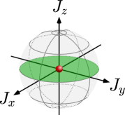
Thus, the uncertainty ellipse of the collective angular momentum is a “pancake” which has zero width in the -direction, while in - and -directions its width is large, as it can be seen in Fig. 2(a) 444Here, the principal axes of the ellipses correspond to the eigenvectors of the covariance matrix It is also usual to plot the SU(2) Wigner function on the Bloch sphere, which can be displayed as a ring on the equator of the Bloch sphere [22]..
(a) (b)
(c)
3.2 Bipartite quantities
In order to detect bipartite entanglement in the Dicke state, we divide the ensemble of particles into two groups (here without partition noise). The corresponding collective angular momentum components are
| (67) |
where .
Assuming even , we introduce the notation
| (68) |
where The value corresponds to dividing the ensemble into two equal halves. The corresponding total spins are
| (69) |
Let us calculate now relevant quantities for the Dicke state spilt into two halves.
For the variance of we obtain
| (70) |
while for the variance of defined in Eq. (19), we obtain
| (71) |
for where the covariance is defined in Eq. (41). Clearly, for the Dicke state, for all expectation values in the two parts we have
| (72) |
for and
From Eq. (66), we obtain
| (73) |
For large , this is about half of the maximum for any quantum state, which is
The variances of the difference of the angular momentum components of the two parts are
| (74) |
which is proved in Appendix C. Let us consider the case separately, for which
| (75) |
As a comparison, for the fully polarized state we get
| (76) |
The variance in Eq. (75) is smaller than Eq. (76). Note also that if is nonzero, then grows rapidly with as can be seen from Eq. (74).
Finally, from Eq. (64), we obtain for the variance of the sum of the -components
| (77) |
That is, the variance of is minimal for Dicke states.
3.3 Bipartite quantities after splitting in an experiment
Let us consider now the splitting that happens in the experiment, which (neglecting the role of particle-particle interactions) mimics a beam-splitter transformation. We will calculate various expectation values for the Dicke state for that case. So far, we assumed that the total particle number and also the particle numbers in the two subsystems, and are constants. Consequently, we also assumed that and are constants. In practice, an experiment must be repeated several times in order to obtain sufficient data, and the total particle number is varying from experiment to experiment. Moreover, even if the total particle number remained constant, when the condensate is split into two parts, we do not obtain two subensembles with exactly particles, but the local particle numbers fluctuate due to partition noise.
If technical noise sources are sufficiently suppressed then the probability of having particles in subsystem is given by the binomial formula
| (78) |
For an ensemble that on average is split equally, the expectation value of is zero. However, the number of particles in the two subsystems fluctuate from experiment to experiment. This is described by the variance of the particle number in the subsystem or the variance of which is
| (79) |
Now we present some quantities after splitting with partition noise, where the expectation values are obtained via an averaging of the expectation values obtained for various values with a weight given in Eq. (78). The derivations are in Appendix D (see also Ref. [85]). The local second moments are
| (80a) | |||||
| (80b) | |||||
for where means averaging over the different values. The correlations are
| (81a) | |||||
| (81b) | |||||
With these, based on Eq. (40), we obtain the coefficients for the Dicke states as in Eq. (42). For simplicity, we will use without the subscript in the future. It will be clear from the context, when expectation values and variances are based on an averaging over various values.
After the correlations, let us write now the collective variances. Based on Eq. (74), they are obtained as
| (82) |
for 555 always if a symmetric state is split with partition noise. See Ref. [85].. Comparing this to Eq. (75), we can see that the collective variance became around twice larger due to the partition noise appearing during the splitting of the condensate. This is an unwelcome effect that reduces the quality of the experimental data, and makes the detection of correlations in split states more difficult.
3.4 Bipartite quantities with the normalized spin components
Here, we consider a normalization of the collective angular momentum components of the subensembles, since it reduces the unwelcome effects of particle number fluctuations. We calculate some spin expectation values for the Dicke state using a normalization factor, and we show that it cancels the effect of the partition noise. Concretely, we consider the normalized quantities
| (83) |
for and Note that normalized operators appear in the context of fluctuators [86, 87, 88, 89], or in modeling spin systems when normalized angular momentum components perpendicular to the mean spin play the role of the operators and of a single mode system [90]. However, the angular momentum components are normalized with a different function of the particle number.
Let us also define for . For their variances on the Dicke state we obtain
| (84) |
which is shown in Appendix E.
Let us calculate the value for an equal splitting, corresponding to We obtain
| (85) |
We now calculate the value taking into account the variance of while the condensate is split. In this case, the variance of is given in Eq. (79), hence In Eq. (84), in the denominator we have
| (86) |
if is large. Hence, we obtain Eq. (85), the same value we would get for an equal splitting with Thus, the fact that the particle number variance after splitting is nonzero did not increase the value of the normalized variance. Remember that the corresponding collective variance without a normalization increased a lot due to the nonzero particle number variance during splitting, as it can be seen in Eq. (82) when compared to Eq. (75).
Note that we define normalized spin components only for the - and -directions, not in the -direction. The reason is that the variance for depends on the splitting ratio while does not.
Finally, let us see now a qualitative argument why the normalization is needed to remove the noise due to splitting with partition noise. For large for the Dicke state we have
| (87) |
for In Eq. (87), for the two terms appearing in the difference we have
| (88) |
Thus, in Eq. (87) we have the difference of two quantities that almost cancel each other, and the difference is much smaller than the quantities themselves. This is the reason that Eq. (87) is so sensitive to the as shown in Eq. (74).
3.5 Entanglement criteria with normalized quantities
Next, we present a formulation of our criteria with normalized spin components. The criteria with normalized quantities are more resistant to partition noise, at least in the case of Dicke states (see Sec. 3.4), and are thus recommended for an experimental use. In short, they can be simply derived repeating the steps described in Sec. 2.2 and Sec. 2.3, after the normalization is inserted in the formulas.
First, we present an EPR steering criterion with normalized quantities.
Observation 7. The following EPR steering criterion holds with the normalized quantities
| (89) |
and can be used for Dicke states. A more general form is
| (90) |
Substituting
| (91) |
Proof. A relation analogous to the one given in Eq. (12) can be written with normalized operators as
| (92) |
for Following steps similar to those in the proof of Observation 2, we obtain the criteria presented in the Observation.
Next, we will present entanglement conditions with normalized quantities.
Observation 8. The following inequality with normalized quantities
| (93) |
holds for separable bipartite states. Here, we defined for
Proof. A relation analogous to the one given in Eq. (47) can be written with normalized operators as
| (94) |
Then, we have to apply Eq. (55) with to obtain an expression that does not have a square root within the expectation value. Here where for large we have
Observation 9. The following inequality with normalized quantities
| (95) |
holds for separable bipartite states.
Proof. We start from the entanglement criterion Eq. (94). Then, we have to apply
| (96) |
which can be proved similarly to Eq. (61). Then, we obtain an expression that does not have a square root within the expectation value.
| Quantum state | LHS/RHS | |||
|---|---|---|---|---|
| Quantum state | LHS/RHS | |||
|---|---|---|---|---|
4 Application of the entanglement criterion for further quantum states and experimentally prepared Dicke states
In this section, we examine how our EPR steering criterion and entanglement criterion work for various ideal quantum states, as well as for a Dicke state prepared experimentally.
4.1 Testing EPR steering and entanglement for various ideal quantum states
We calculate the relevant normalized quantities for the EPR steering criterion given in Eq. (90) and the entanglement criterion given in Eq. (93) for various quantum states. The results for the EPR condition are shown in Table 2. The quantities presented in the table are the sum of variances in subsystem
| (97) |
and the sum of second moments in subsystem
| (98) |
The criterion given in Eq. (90) can be written as
| (99) |
with the quantities given in the table.
The results for the entanglement condition are shown in Table 2. The quantities presented in the table are the variances of the differences between the two subsystems
| (100) |
and the sum of global second moments
| (101) |
The criterion given in Eq. (93) can be written as
| (102) |
with the quantities given in the table.
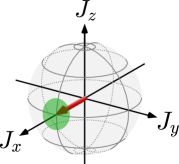
The Dicke state violates both criteria very strongly. The state with all spins pointing into the -direction, depicted in Fig. 2(b), is close to saturate both relations. All examples are valid when the ensemble is split with partition noise, and also for the case when the ensemble is divided into two equal halves without such noise. For the Dicke state, based on the arguments presented in this paper, there is not an observable difference between the two cases for large particle numbers since we used normalized quantities. For the product states, straightforward arguments also show that there is not an observable difference for large particle numbers. Next we discuss, what estimates we used for the various states in the criterion given in Eqs. (97) and (99). For the Dicke state, we used the estimates given in Eq. (91). The other states were product states, hence we used
| (103) |
4.2 Experimental results with Dicke states
Next, we test our entanglement criterion with experimental data from Ref. [60]. There, a Dicke state of around 8000 atoms was prepared, and bipartite entanglement was detected after splitting. However, in that work a different entanglement criterion was used. Due to the characteristics of the setup, they could measure in the two subsystems. They could also measure
| (104) |
where and is a random angle with a uniform probability distribution between and Note that at a given measurement, the angle is the same for and
Let us now consider the normalized quantities
| (105) | ||||
The average moment of the angular momentum in the -plane is defined as
| (106) |
It is easy to see that the average second moment can be expressed, rather than with an integral, as an average of two operators, namely
| (107) |
while the first moment is zero Equation (107) can be derived knowing that for the second moments
| (108) |
holds, while for the correlations we have
| (109) |
which can be proved with straightforward algebra.
With these, the entanglement criterion given in Eq. (93) can be rewritten as
| (110) |
In the experiment described in Ref. [60], they used as point of reference the values obtained for the state fully polarized in the -direction given as
| (111) |
In Table 2, it can be seen that this state is very close to saturate the entanglement criterion Eq. (93) for large In the experiment described in Ref. [60], is much smaller than The reason is that the process that prepares the Dicke state ideally creates the eigenstate of with eigenvalue that is, ideally we have On the other hand, is larger than and the state is close to be symmetric. We plotted the results in Fig. 3(a).
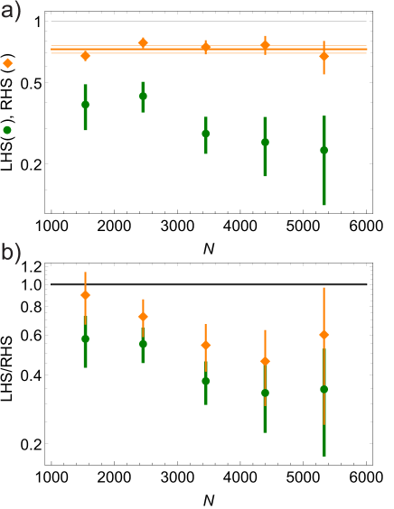
We can see that the experimental values violate the condition given in Eq. (110). The inequality presented in this paper is more sensitive than the one presented in Ref. [60]. We can now observe the main characteristics of our method. First, we don’t need to assume that the quantum state is fully symmetric. Furthermore, our method can handle particle number variance from experiment to experiment. In practice, the criterion is robust enough to detect entanglement in an actual experiment, where, although the variance of can be very close to zero, can be much larger than for the ideal Dicke state. Hence, an entanglement criterion with the product of these two quantities could be more efficient than a criterion with their sum. In Appendix F, we present some simple entanglement criteria for two spins, which are not yet practical, that help to understand how we developed our criteria.
4.3 Application of the entanglement condition for split spin-squeezed states
From Sec. 4.1 we could see that the state fully polarized in the -direction was close to saturate the entanglement criterion Eq. (93). Now, if we start from this state, and apply some suitable interaction between the particles, we can obtain a spin-squeezed state, which has a reduced uncertainty along some direction orthogonal to the mean spin. Such states are entangled, and they are useful, e.g., for quantum metrology, where they outperform separable states [91, 92, 17]. Spin-squeezed states are now routinely prepared in experiments, and their entanglement has been detected in cold atomic ensembles [43, 45, 46, 47] and in BECs [42, 50, 52, 53, 54]. In addition, collective measurements allowed to detect and quantify even Bell correlations in such states [93, 94, 95, 96]. On the other hand, the use of local spin measurements in BECs allowed to detect entanglement and EPR steering between parts of a spin-squeezed state [71, 69].
Here, we show that our entanglement criterion detects bipartite entanglement in split spin-squeezed states. Such states can be created starting from a spin coherent state polarized along the -direction. Then, we apply a dynamics governed by the one-axis twisting Hamiltonian
| (114) |
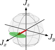
where defines the interaction strength. The state can be parametrized during the evolution by the adimensional parameter where is the evolution time. With this parametrization we follow the notation of Ref. [91]. The state has a reduced spin variance along some direction in the -plane. By applying a rotation around the -axis, one can orient the state such that the variance is smallest along the -direction. Figures 2(b) and (c) show the spin and the uncertainty ellipses of the states fully polarized in the -direction and of the state that is also spin-squeezed in the -direction.
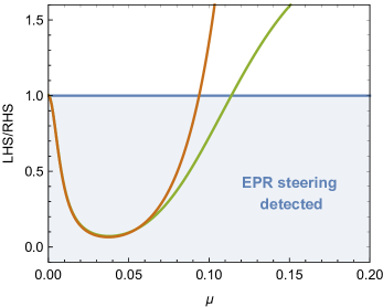
Let us now consider a splitting of the state into two halves with equal particle numbers, and investigate correlations between them. The calculations can be simplified since the state is in the symmetric subspace. The resulting bipartite state has been presented in Refs. [69, 97], and it allows us to evaluate analytically Eq. (90), which is plotted in Fig. 4. By comparing the violation of the Reid criterion for spins, Eq. (25), and of the EPR steering criterion presented in this paper, Eq. (90), we observe that the latter allows us to detect steering for a wider range of This is the case, because our criterion remains sensitive even when the anti-squeezed component starts to spread around the Bloch sphere.
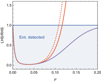
In Fig. 5, we show similar curves for the entanglement criterion given in Eq. (93). We compare our approach to the criterion given in Eq. (45) with and which is based on the paper of Giovannetti et al. given in Ref. [72] (see also Ref. [69]). We can see that our criterion allows us to detect spin-squeezed states as entangled even for large values where the state is significantly non-Gaussian.
In Fig. 5, we also show the results with the criterion given in Eq. (93) for the case of splitting with partition noise. The curve for such case however overlaps with the curve corresponding to equal splitting. Thus, normalization can the help a lot to mitigate the effects of partition noise.
In summary, our criteria for bipartite entanglement developed for the unpolarized Dicke state work also for other classes of states, such as spin-squeezed states. Note that this is similar to the criteria for multipartite entanglement developed for Dicke states in Ref. [24], that were also applicable for spin-squeezed states [25].
5 Discussion
In this section, we compare our approach to other works about detecting entanglement in bipartite systems. While bipartite entanglement has been detected in many-particle systems in photons [98, 99, 100, 58] and cold atomic ensembles [46], we consider now in more detail recent works that discuss how to detect bipartite entanglement in Bose-Einstein condensates of cold atoms.
Some of the proposals are based on detecting bipartite entanglement in split spin-squeezed states, also discussed in Sec. 4.3. In such systems, the originally fully polarized state of two-state atoms becomes entangled due to an interaction and the variance of a collective spin component, orthogonal to the mean spin, decreases. In Ref. [101], they derive entanglement witnesses using either only first-order or both first- and second-order moments of local collective spin components. In both cases, they derive optimal witnesses for spatially split spin-squeezed states in the presence of local white noise. The correlation-based witness presented is also discussed in Appendix F.1. In Ref. [102], it is discussed how to detect bipartite nonlocality in spin systems based on parity measurements, essentially, based on measuring higher-order moments. Experimentally, the observation of EPR correlations between spatially separated modes was achieved in split-squeezed atomic ensembles [71], using a criterion developed by Giovannetti et al. in Ref. [72].
Other works consider three-state atoms, originally in the state and an interaction in which pairs of atoms from tunnel to the and states [103]. In such systems, two operators, different from the angular momentum components, have been presented that have a commutation relation similar to those of the canonical and operators, and make it possible to detect spin-nematic squeezing. Based on the ideas above, EPR correlations have been detected experimentally [73].
Finally, if after the dynamics mentioned above we project to the subspace with fixed number atoms in states and then we obtain a Dicke state given in Eq. (1). It is a highly entangled multi-qubit state that has many advantageous properties discussed in Appendix A. A key fact is that for the Dicke state the expectation value of all the spin components is zero, thus the criteria must contain the second moment of the spin components. Ref. [60] presents an experiment in which entanglement has been detected in such systems with the measurement of collective angular momentum components in the two parties. Our article derives an independent criterion based on general principles, which seems to be stronger when tested on experimental data, as can be seen in Fig. 3(b). A key difference is that the present criterion given in Eq. (110) includes the term given in Eq. (107), which provides information on how much the bipartite quantum state is in the symmetric subspace. The criterion given in Ref. [60] has this type of information only about the subsystems. In the present paper, we also show in detail how the normalization of the spin components cancel some of the partition noise. We also present a criterion for EPR entanglement for Dicke states. We also show that, apart from Dicke states, our criteria work also for split spin-squeezed states.
Conclusions
We presented an uncertainty relation that plays the role of number-phase uncertainty for atomic systems. Based on this uncertainty relation, we described methods to detect Einstein-Podolsky-Rosen steering and bipartite entanglement. Our methods are especially suited for Dicke states, which gave us the motivation for this work, however, they can be also applied to other experimentally relevant states, for instance, split spin-squeezed states. Our methods can handle imperfections, such a nonzero particle number variance, including the partition noise. They can also handle the problem that the quantum state does not live in a single spatial mode since the populations of the other modes are not fully suppressed. When applied to split nonclassical states, all these conditions need collective spin measurements in the two halves of the system, which are routinely measured in atomic gases and BECs. In the future, it would be interesting to estimate entanglement monotones based on the measured violation of the entanglement criteria [74].
Appendix A The Dicke state as a bipartite state
In this Appendix, we analyze the entanglement properties of Dicke states given in Eq. (1). First of all, the entanglement of Dicke states is quite robust to external noise and imperfections. For instance, loosing a particle does not make the Dicke state separable. As already mentioned, Dicke states make possible quantum metrology with the maximal, Heisenberg scaling [20].
The entanglement of formation of is known considering an equal partitioning of the particles [75]. For large it is given as
| (115) |
In comparison, the entanglement of a maximally entangled state of two qudits of dimension is Hence, the bipartite entanglement of the Dicke state is close to the entanglement of a maximally entangled state with
Let us observe this in more detail. The Schmidt decomposition of the Dicke state is [75, 104]
| (116) |
where the coefficients are
| (117) |
and the basis states in the two subsystems are
| (118) |
The states given in Eq. (118) are symmetrized superpositions of all product states with 1’s and 0’s.
Let us now consider an equal splitting, which means
| (119) |
While the state has nonzero Schmidt coefficients, most of these coefficients are close to zero since for large the binomial can be approximated with a Gaussian and we obtain
| (120) |
Hence, is large if
| (121) |
This explanation made it easier to understand Eq. (115) qualitatively.
It is instructive to compare Dicke states to the celebrated Greenberger-Horne-Zeilinger (GHZ) states [105]
| (122) |
which play a central role in quantum information science. GHZ states have been realized in photonic systems [106, 107, 108, 109, 110] and in cold trapped ions [111, 112, 113]. GHZ states make possible quantum metrology with the maximal, Heisenberg scaling [111].
GHZ states have a bipartite entanglement of the two halves of the particles equal to
| (123) |
Moreover, the entanglement of GHZ states is fragile, and the loss of a single particle can lead to a trivial separable state. GHZ states have been created successfully up to 10-20 particles.
Appendix B Relation to number-phase uncertainty
In this section, we attempt to connect our derivation to the literature on number-phase uncertainty relations [114, 115, 116, 117, 118, 119, 120, 121]. If the system is described by a bosonic mode then the number phase relation is written such that the phase operator is related to the annihilation operator of the mode. Such systems are, for example, light fields, where the superposition of states with different number of photons is detectable. An alternative of the number-phase uncertainty has been used to detect entanglement in two-mode systems [122, 123]. An entanglement criterion related to the number-phase uncertainty for two photonic modes, such that one of the modes have few photons, has been considered [124]. An EPR steering criterion has been presented in such system for two modes [125].
However, in our case we have massive particles. The superposition of quantum states with different particle numbers is not detectable. In other words, the particle number is preserved by the measurements. In the case of two bosonic modes (e.g., two energy levels), this situation can be handled by mapping the bosonic modes to a spin ensemble using the Schwinger representation [121, 123]
| (124) |
where are the two modes corresponding to two internal states of the particles. In this case, the role of the annihilation operator in the number-phase uncertainty relation is played by the operator
| (125) |
The operator describes a process in which particles move from one mode to the other, thus the total particle number does not change.
Based on these, an uncertainty relation resembling a number-phase uncertainty has been obtained between and the operator defined via the relation [121]
| (126) |
where which can be further rewritten as
| (127) |
Since the angular momentum operators are defined with the Schwinger representation for two bosonic modes, the description above is appropriate to describe quantum states of two-state particles with a bosonic symmetry. However, it does not describe general quantum states of particles that are not symmetric.
We can interpret our approach as one that defines a similar operator
| (128) |
where the operators and are defined as
| (129) |
which are operators roughly corresponding to cosine and sine of the phase. Note that we assume that the quantum state is a multi-qubit state, not necessarily with a bosonic symmetry, and are just the sums of the single-particle spin components as in Eq. (5). We can rewrite Eq. (12) with these operators as
| (130) |
Appendix C Derivation of Eq. (74)
In this Appendix, we calculate various quantities for the Dicke state given in Eq. (1). We obtain two-particle and bipartite correlations, and at the end we derive Eq. (74).
We will now calculate two-particle correlations of the Dicke state. Due to the permutational invariance
| (131) |
holds for and for all Hence,
| (132) |
Then, based on Eqs. (66) and (132)
| (133) |
for while using Eq. (64) we obtain
| (134) |
Using Eq. (67), we write the correlations between collective angular momentum component of the two halves with the two-body correlations as
| (135) |
for Hence, using Eqs. (133) and (134), we obtain for the correlations between the left and right halves
| (136a) | |||||
| (136b) | |||||
Note that if we measure or on both sides, the measurement results will be correlated with each other. If we measure on both sides, the measurement results will be anticorrelated with each other.
It is worth to calculate the maximum of the correlations for any state. We obtain
| (137) |
where the bound is sharp. Note that for large the correlations given in Eq. (136a) are only twice less than the absolute maximum given in Eq. (137) for Thus, the Dicke state has strong correlations both in the - and -directions.
Appendix D Quantities after splitting with partition noise
In this Appendix, we calculate various quantities based on the splitting with partition noise characterized by Eq. (79).
In order to proceed, we need that
| (139) |
for and where we used that The two-point correlations are given in Eqs. (133) and (134). Hence, based on Eq. (69) we obtain
for Now, considering Eq. (79) we arrive at Eq. (80). Based on Eq. (136), the correlations are obtained as in Eq. (81).
Appendix E Derivation of the formula for the variance using normalized quantities, given in Eq. (84)
In this Appendix, we calculate various quantities for the Dicke state given in Eq. (1), in order to derive Eq. (84). Based on Eq. (139), the normalized second moments are obtained as
| (141) |
for and The two-point correlations are given in Eq. (133).
Let us consider the difference between the normalized collective angular momentum components of the two subsystems, denoted by . For its variance, we obtain
| (142) |
which leads to Eq. (84). Here, in the first equality we used Eq. (72), which results in and we used Eq. (135) giving the correlations. For the second, approximate equality we used the two-body correlations given in Eq. (133) and the normalized second moments given in Eq. (141). We also used
| (143) |
which is based on that holds for small
Appendix F Basic ideas concerning entanglement detection
In this section, we present simple criteria that detect the Dicke state given in Eq. (1) as entangled. These criteria are not yet practical, but will help us to understand the main problems of entanglement detection in such systems.
Next, we assume that the states in the two subsystems are symmetric. Ideally, we can expect this, since the Dicke state is a symmetric multipartite state. If we split it into two subsystems, the quantum state within the subsystems is also symmetric. Hence, the quantum state can be mapped into a quantum state of two large spins.
Based on Eqs. (136) and (79), the correlation between the two halves are obtained as in Eq. (81). The values given in Eq. (81) are very close to the values given in Eq. (136), if we consider large and substitute Thus, the fact that there is a nonzero particle number variance during the splitting does not change these correlations a lot compared to the case when the atoms are split into two perfectly equal halves.
F.1 Criterion based on correlations
Since we have a bipartite system, a first straightforward idea is to detect entanglement based on the correlations between the two parties. For instance, for separable states of two qubits
| (144) |
holds [126, 127, 128]. For two spin- particles a similar relation can be obtained as
| (145) |
Let us consider now our Dicke state split into two equal halves. Since the state is in the symmetric subspace, we can map it into a state of two particles of spin and Then, the entanglement condition reads as
| (146) |
where we have used Eq. (69). Knowing that in the experiment the variance of is given by Eq. (79), we obtain
| (147) |
which has been derived in Ref. [101]. (Note that Ref. [101] presented further interesting results.)
Based on Eq. (136), for the ideal Dicke state the left-hand side of Eq. (146) is
| (148) |
If we consider the splitting for which Eq. (79) holds, then for the left-hand side of Eq. (146) we obtain
| (149) |
The value for the Dicke state given in Eq. (149) is very close to the bound given on the right-hand side of Eq. (147). Hence, it is difficult to use the criterion for a real experiment. In fact, both the value for Dicke states and the bound is in leading order in while their difference is proportional to in leading order in
F.2 Criterion based on variances
Next, we present simple criteria that use the variances of collective observables. As an introduction, let us consider a well known criterion aimed at detecting singlet states. For separable states of a bipartite system corresponding to the partition [78],
| (150) |
holds. For singlet states, the left-hand side of Eq. (150) is zero, hence they maximally violate the condition.
We would like to apply a similar idea to Dicke states. Hence, we modify the relation
| (151) |
The bound for separable states remain the same, however, now the Dicke state violates Eq. (151). For Dicke states, based on Eq. (74), the left-hand side is
| (152) |
For the case, representing equal splitting, the Dicke state is detected as entangled. However, the criterion is not very robust. If our Dicke state has ideal correlations in the - and -directions then can grow up to around such that the Dicke state is still detected. Conversely, if the correlations in the -direction are perfect, then can grow by around a factor of to and the state is still detected as entangled. Thus, the criterion tolerates very low noise in
References
- [1] Otfried Gühne and Géza Tóth. “Entanglement detection”. Phys. Rep. 474, 1–75 (2009).
- [2] Ryszard Horodecki, Paweł Horodecki, Michał Horodecki, and Karol Horodecki. “Quantum entanglement”. Rev. Mod. Phys. 81, 865–942 (2009).
- [3] Nicolai Friis, Giuseppe Vitagliano, Mehul Malik, and Marcus Huber. “Entanglement certification from theory to experiment”. Nat. Rev. Phys. 1, 72–87 (2019).
- [4] Irénée Frérot, Matteo Fadel, and Maciej Lewenstein. “Probing quantum correlations in many-body systems: a review of scalable methods” (2023). arXiv:2302.00640.
- [5] Luca Pezzé and Augusto Smerzi. “Entanglement, nonlinear dynamics, and the Heisenberg limit”. Phys. Rev. Lett. 102, 100401 (2009).
- [6] Philipp Hyllus, Wiesław Laskowski, Roland Krischek, Christian Schwemmer, Witlef Wieczorek, Harald Weinfurter, Luca Pezzé, and Augusto Smerzi. “Fisher information and multiparticle entanglement”. Phys. Rev. A 85, 022321 (2012).
- [7] Géza Tóth. “Multipartite entanglement and high-precision metrology”. Phys. Rev. A 85, 022322 (2012).
- [8] Robert Raussendorf and Hans J. Briegel. “A one-way quantum computer”. Phys. Rev. Lett. 86, 5188–5191 (2001).
- [9] Robert Raussendorf, Daniel E. Browne, and Hans J. Briegel. “Measurement-based quantum computation on cluster states”. Phys. Rev. A 68, 022312 (2003).
- [10] Daniel Gottesman. “Class of quantum error-correcting codes saturating the quantum hamming bound”. Phys. Rev. A 54, 1862–1868 (1996).
- [11] Richard Cleve, Daniel Gottesman, and Hoi-Kwong Lo. “How to share a quantum secret”. Phys. Rev. Lett. 83, 648–651 (1999).
- [12] Marcos Curty, Maciej Lewenstein, and Norbert Lütkenhaus. “Entanglement as a precondition for secure quantum key distribution”. Phys. Rev. Lett. 92, 217903 (2004).
- [13] Peter W. Shor. “Polynomial-time algorithms for prime factorization and discrete logarithms on a quantum computer”. SIAM Review 41, 303–332 (1999).
- [14] L. K. Grover. “A fast quantum mechanical algorithm for database search” (1996). arXiv:quant-ph/9605043.
- [15] L. Diósi. “Models for universal reduction of macroscopic quantum fluctuations”. Phys. Rev. A 40, 1165–1174 (1989).
- [16] Florian Fröwis and Wolfgang Dür. “Measures of macroscopicity for quantum spin systems”. New J. Phys. 14, 093039 (2012).
- [17] Anders S. Sørensen and Klaus Mølmer. “Entanglement and extreme spin squeezing”. Phys. Rev. Lett. 86, 4431–4434 (2001).
- [18] Géza Tóth, Christian Knapp, Otfried Gühne, and Hans J. Briegel. “Optimal spin squeezing inequalities detect bound entanglement in spin models”. Phys. Rev. Lett. 99, 250405 (2007).
- [19] Géza Tóth, Christian Knapp, Otfried Gühne, and Hans J. Briegel. “Spin squeezing and entanglement”. Phys. Rev. A 79, 042334 (2009).
- [20] Bernd Lücke, Manuel Scherer, Jens Kruse, Luca Pezzé, Frank Deuretzbacher, Phillip Hyllus, Jan Peise, Wolfgang Ertmer, Jan Arlt, Luis Santos, Agosto Smerzi, and Carsten Klempt. “Twin matter waves for interferometry beyond the classical limit”. Science 334, 773–776 (2011).
- [21] Géza Tóth and Iagoba Apellaniz. “Quantum metrology from a quantum information science perspective”. J. Phys. A: Math. Theor. 47, 424006 (2014).
- [22] Luca Pezzè, Augusto Smerzi, Markus K. Oberthaler, Roman Schmied, and Philipp Treutlein. “Quantum metrology with nonclassical states of atomic ensembles”. Rev. Mod. Phys. 90, 035005 (2018).
- [23] L.-M. Duan. “Entanglement detection in the vicinity of arbitrary dicke states”. Phys. Rev. Lett. 107, 180502 (2011).
- [24] Bernd Lücke, Jan Peise, Giuseppe Vitagliano, Jan Arlt, Luis Santos, Géza Tóth, and Carsten Klempt. “Detecting multiparticle entanglement of Dicke states”. Phys. Rev. Lett. 112, 155304 (2014).
- [25] Giuseppe Vitagliano, Iagoba Apellaniz, Matthias Kleinmann, Bernd Lücke, Carsten Klempt, and Géza Tóth. “Entanglement and extreme spin squeezing of unpolarized states”. New J. Phys. 19, 013027 (2017).
- [26] Z. Zhang and L. M. Duan. “Quantum metrology with dicke squeezed states”. New J. Phys. 16, 103037 (2014).
- [27] Iagoba Apellaniz, Bernd Lücke, Jan Peise, Carsten Klempt, and Géza Tóth. “Detecting metrologically useful entanglement in the vicinity of Dicke states”. New J. Phys. 17, 083027 (2015).
- [28] Iagoba Apellaniz, Matthias Kleinmann, Otfried Gühne, and Géza Tóth. “Optimal witnessing of the quantum Fisher information with few measurements”. Phys. Rev. A 95, 032330 (2017).
- [29] L.-M. Duan, J. I. Cirac, and P. Zoller. “Quantum entanglement in spinor Bose-Einstein condensates”. Phys. Rev. A 65, 033619 (2002).
- [30] Giuseppe Vitagliano, Philipp Hyllus, Iñigo L. Egusquiza, and Géza Tóth. “Spin squeezing inequalities for arbitrary spin”. Phys. Rev. Lett. 107, 240502 (2011).
- [31] Giuseppe Vitagliano, Iagoba Apellaniz, Iñigo L. Egusquiza, and Géza Tóth. “Spin squeezing and entanglement for an arbitrary spin”. Phys. Rev. A 89, 032307 (2014).
- [32] Géza Tóth and Morgan W. Mitchell. “Generation of macroscopic singlet states in atomic ensembles”. New J. Phys. 12, 053007 (2010).
- [33] J. Ma, X. Wang, C. P. Sun, and F. Nori. “Quantum spin squeezing”. Phys. Rep. 509, 89–165 (2011).
- [34] N. Kiesel, C. Schmid, G. Tóth, E. Solano, and H. Weinfurter. “Experimental observation of four-photon entangled Dicke state with high fidelity”. Phys. Rev. Lett. 98, 063604 (2007).
- [35] Witlef Wieczorek, Roland Krischek, Nikolai Kiesel, Patrick Michelberger, Géza Tóth, and Harald Weinfurter. “Experimental entanglement of a six-photon symmetric Dicke state”. Phys. Rev. Lett. 103, 020504 (2009).
- [36] R. Prevedel, G. Cronenberg, M. S. Tame, M. Paternostro, P. Walther, M. S. Kim, and A. Zeilinger. “Experimental realization of Dicke states of up to six qubits for multiparty quantum networking”. Phys. Rev. Lett. 103, 020503 (2009).
- [37] Roland Krischek, Christian Schwemmer, Witlef Wieczorek, Harald Weinfurter, Philipp Hyllus, Luca Pezzé, and Augusto Smerzi. “Useful multiparticle entanglement and sub-shot-noise sensitivity in experimental phase estimation”. Phys. Rev. Lett. 107, 080504 (2011).
- [38] A. Chiuri, C. Greganti, M. Paternostro, G. Vallone, and P. Mataloni. “Experimental quantum networking protocols via four-qubit hyperentangled dicke states”. Phys. Rev. Lett. 109, 173604 (2012).
- [39] Justin G. Bohnet, Brian C. Sawyer, Joseph W. Britton, Michael L. Wall, Ana Maria Rey, Michael Foss-Feig, and John J. Bollinger. “Quantum spin dynamics and entanglement generation with hundreds of trapped ions”. Science 352, 1297–1301 (2016).
- [40] H. Häffner, W. Hänsel, C. F. Roos, J. Benhelm, M. Chwalla, T. Körber, D. Rapol, U, M. Riebe, P. O. Schmidt, C. Becher, O. Gühne, W. Dür, and R. Blatt. “Scalable multiparticle entanglement of trapped ions”. Nature (London) 438, 643–646 (2005).
- [41] D. B. Hume, C. W. Chou, T. Rosenband, and D. J. Wineland. “Preparation of Dicke states in an ion chain”. Phys. Rev. A 80, 052302 (2009).
- [42] Christian Gross. “Spin squeezing, entanglement and quantum metrology with bose–einstein condensates”. J. Phys. B: At. Mol. Opt. Phys. 45, 103001 (2012).
- [43] W. Wasilewski, K. Jensen, H. Krauter, J. J. Renema, M. V. Balabas, and E. S. Polzik. “Quantum noise limited and entanglement-assisted magnetometry”. Phys. Rev. Lett. 104, 133601 (2010).
- [44] T. Fernholz, H. Krauter, K. Jensen, J. F. Sherson, A. S. Sørensen, and E. S. Polzik. “Spin squeezing of atomic ensembles via nuclear-electronic spin entanglement”. Phys. Rev. Lett. 101, 073601 (2008).
- [45] J. Hald, J. L. Sørensen, C. Schori, and E. S. Polzik. “Spin squeezed atoms: A macroscopic entangled ensemble created by light”. Phys. Rev. Lett. 83, 1319–1322 (1999).
- [46] Brian Julsgaard, Alexander Kozhekin, and Eugene S Polzik. “Experimental long-lived entanglement of two macroscopic objects”. Nature (London) 413, 400–403 (2001).
- [47] Klemens Hammerer, Anders S. Sørensen, and Eugene S. Polzik. “Quantum interface between light and atomic ensembles”. Rev. Mod. Phys. 82, 1041–1093 (2010).
- [48] N. Behbood, F. Martin Ciurana, G. Colangelo, M. Napolitano, Géza Tóth, R. J. Sewell, and M. W. Mitchell. “Generation of macroscopic singlet states in a cold atomic ensemble”. Phys. Rev. Lett. 113, 093601 (2014).
- [49] Jia Kong, Ricardo Jiménez-Martínez, Charikleia Troullinou, Vito Giovanni Lucivero, Géza Tóth, and Morgan W. Mitchell. “Measurement-induced, spatially-extended entanglement in a hot, strongly-interacting atomic system”. Nat. Commun. 11, 2415 (2020).
- [50] J. Esteve, C. Gross, A. Weller, S. Giovanazzi, and M. K. Oberthaler. “Squeezing and entanglement in a Bose–Einstein condensate”. Nature (London) 455, 1216–1219 (2008).
- [51] Christian Gross, Tilman Zibold, Eike Nicklas, Jerome Esteve, and Markus K Oberthaler. “Nonlinear atom interferometer surpasses classical precision limit”. Nature (London) 464, 1165–1169 (2010).
- [52] Max F. Riedel, Pascal Böhi, Yun Li, Theodor W. Hänsch, Alice Sinatra, and Philipp Treutlein. “Atom-chip-based generation of entanglement for quantum metrology”. Nature (London) 464, 1170–1173 (2010).
- [53] Caspar F. Ockeloen, Roman Schmied, Max F. Riedel, and Philipp Treutlein. “Quantum metrology with a scanning probe atom interferometer”. Phys. Rev. Lett. 111, 143001 (2013).
- [54] W. Muessel, H. Strobel, D. Linnemann, D. B. Hume, and M. K. Oberthaler. “Scalable spin squeezing for quantum-enhanced magnetometry with Bose-Einstein condensates”. Phys. Rev. Lett. 113, 103004 (2014).
- [55] C. D. Hamley, C. S. Gerving, T. M. Hoang, E. M. Bookjans, and M. S. Chapman. “Spin-nematic squeezed vacuum in a quantum gas”. Nat. Phys. 8, 305–308 (2012).
- [56] Yi-Quan Zou, Ling-Na Wu, Qi Liu, Xin-Yu Luo, Shuai-Feng Guo, Jia-Hao Cao, Meng Khoon Tey, and Li You. “Beating the classical precision limit with spin-1 Dicke states of more than 10,000 atoms”. Proc. Natl. Acad. Sci. U.S.A. 115, 6381–6385 (2018).
- [57] N. Killoran, M. Cramer, and M. B. Plenio. “Extracting entanglement from identical particles”. Phys. Rev. Lett. 112, 150501 (2014).
- [58] Mario Krenn, Marcus Huber, Robert Fickler, Radek Lapkiewicz, Sven Ramelow, and Anton Zeilinger. “Generation and confirmation of a (100 100)-dimensional entangled quantum system”. Proc. Natl. Acad. Sci. U.S.A. 111, 6243–6247 (2014).
- [59] Paul Erker, Mario Krenn, and Marcus Huber. “Quantifying high dimensional entanglement with two mutually unbiased bases”. Quantum 1, 22 (2017).
- [60] Karsten Lange, Jan Peise, Bernd Lücke, Ilka Kruse, Giuseppe Vitagliano, Iagoba Apellaniz, Matthias Kleinmann, Géza Tóth, and Carsten Klempt. “Entanglement between two spatially separated atomic modes”. Science 360, 416–418 (2018).
- [61] A. Einstein, B. Podolsky, and N. Rosen. “Can quantum-mechanical description of physical reality be considered complete?”. Phys. Rev. 47, 777–780 (1935).
- [62] M. D. Reid. “Demonstration of the Einstein-Podolsky-Rosen paradox using nondegenerate parametric amplification”. Phys. Rev. A 40, 913–923 (1989).
- [63] M. D. Reid. “The Einstein-Podolsky-Rosen Paradox and Entanglement 1: Signatures of EPR correlations for continuous variables” (2001). arXiv:quant-ph/0112038.
- [64] M. D. Reid, P. D. Drummond, W. P. Bowen, E. G. Cavalcanti, P. K. Lam, H. A. Bachor, U. L. Andersen, and G. Leuchs. “Colloquium: The Einstein-Podolsky-Rosen paradox: From concepts to applications”. Rev. Mod. Phys. 81, 1727–1751 (2009).
- [65] E. G. Cavalcanti, S. J. Jones, H. M. Wiseman, and M. D. Reid. “Experimental criteria for steering and the Einstein-Podolsky-Rosen paradox”. Phys. Rev. A 80, 032112 (2009).
- [66] Z. Y. Ou, S. F. Pereira, H. J. Kimble, and K. C. Peng. “Realization of the Einstein-Podolsky-Rosen paradox for continuous variables”. Phys. Rev. Lett. 68, 3663–3666 (1992).
- [67] J. Peise, I. Kruse, K. Lange, B. Lücke, L. Pezzè, J. Arlt, W. Ertmer, K. Hammerer, L. Santos, A. Smerzi, and C. Klempt. “Satisfying the Einstein-Podolsky-Rosen criterion with massive particles”. Nat. Commun. 6, 8984 (2015).
- [68] Q. Y. He, M. D. Reid, T. G. Vaughan, C. Gross, M. Oberthaler, and P. D. Drummond. “Einstein-Podolsky-Rosen entanglement strategies in two-well Bose-Einstein condensates”. Phys. Rev. Lett. 106, 120405 (2011).
- [69] Yumang Jing, Matteo Fadel, Valentin Ivannikov, and Tim Byrnes. “Split spin-squeezed Bose–Einstein condensates”. New J. Phys. 21, 093038 (2019).
- [70] Jiajie Guo, Feng-Xiao Sun, Daoquan Zhu, Manuel Gessner, Qiongyi He, and Matteo Fadel. “Detecting Einstein-Podolsky-Rosen steering in non-Gaussian spin states from conditional spin-squeezing parameters” (2021). arXiv:2106.13106.
- [71] Matteo Fadel, Tilman Zibold, Boris Décamps, and Philipp Treutlein. “Spatial entanglement patterns and Einstein-Podolsky-Rosen steering in Bose-Einstein condensates”. Science 360, 409–413 (2018).
- [72] Vittorio Giovannetti, Stefano Mancini, David Vitali, and Paolo Tombesi. “Characterizing the entanglement of bipartite quantum systems”. Phys. Rev. A 67, 022320 (2003).
- [73] Philipp Kunkel, Maximilian Prüfer, Helmut Strobel, Daniel Linnemann, Anika Frölian, Thomas Gasenzer, Martin Gärttner, and Markus K Oberthaler. “Spatially distributed multipartite entanglement enables EPR steering of atomic clouds”. Science 360, 413–416 (2018).
- [74] Matteo Fadel, Ayaka Usui, Marcus Huber, Nicolai Friis, and Giuseppe Vitagliano. “Entanglement quantification in atomic ensembles”. Phys. Rev. Lett. 127, 010401 (2021).
- [75] John K. Stockton, J. M. Geremia, Andrew C. Doherty, and Hideo Mabuchi. “Characterizing the entanglement of symmetric many-particle spin- systems”. Phys. Rev. A 67, 022112 (2003).
- [76] P. Hyllus, L. Pezzé, and A. Smerzi. “Entanglement and sensitivity in precision measurements with states of a fluctuating number of particles”. Phys. Rev. Lett. 105, 120501 (2010).
- [77] Philipp Hyllus, Luca Pezzé, Augusto Smerzi, and Géza Tóth. “Entanglement and extreme spin squeezing for a fluctuating number of indistinguishable particles”. Phys. Rev. A 86, 012337 (2012).
- [78] Géza Tóth. “Entanglement detection in optical lattices of bosonic atoms with collective measurements”. Phys. Rev. A 69, 052327 (2004).
- [79] Géza Tóth and Florian Fröwis. “Uncertainty relations with the variance and the quantum fisher information based on convex decompositions of density matrices”. Phys. Rev. Research 4, 013075 (2022).
- [80] E. G. Cavalcanti and M. D. Reid. “Uncertainty relations for the realization of macroscopic quantum superpositions and EPR paradoxes”. J. Mod. Opt. 54, 2373–2380 (2007).
- [81] M. D. Reid and Q. Y. He. “Quantifying the mesoscopic nature of Einstein-Podolsky-Rosen nonlocality”. Phys. Rev. Lett. 123, 120402 (2019).
- [82] B. J. Dalton, B. M. Garraway, and M. D. Reid. “Tests for Einstein-Podolsky-Rosen steering in two-mode systems of identical massive bosons”. Phys. Rev. A 101, 012117 (2020).
- [83] R. Bhatia. “Matrix analysis”. Graduate texts in mathematics. Springer, New York. (1997).
- [84] Fumio Hiai and Dénes Petz. “Introduction to matrix analysis and applications”. Springer Science & Business Media. (2014).
- [85] Matteo Fadel and Manuel Gessner. “Relating spin squeezing to multipartite entanglement criteria for particles and modes”. Phys. Rev. A 102, 012412 (2020).
- [86] Zoltan Kadar, Michael Keyl, Geza Toth, and Zoltan Zimboras. “Simulating continuous quantum systems by mean field fluctuations” (2012). arXiv:1211.2173.
- [87] G. A. Raggio and R. F. Werner. “Quantum statistical mechanics of general mean field systems”. Helv. Phys. Acta 62, 980–1003 (1989).
- [88] D. Goderis, A. Verbeure, and P. Vets. “Non-commutative central limits”. Probab. Theory Relat. Fields 82, 527–544 (1989).
- [89] D. Goderis and P. Vets. “Central limit theorem for mixing quantum systems and the CCR-algebra of fluctuations”. Commun. Math. Phys. 122, 249–265 (1989).
- [90] Lu-Ming Duan, J. I. Cirac, P. Zoller, and E. S. Polzik. “Quantum communication between atomic ensembles using coherent light”. Phys. Rev. Lett. 85, 5643–5646 (2000).
- [91] Masahiro Kitagawa and Masahito Ueda. “Squeezed spin states”. Phys. Rev. A 47, 5138–5143 (1993).
- [92] D. J. Wineland, J. J. Bollinger, W. M. Itano, and D. J. Heinzen. “Squeezed atomic states and projection noise in spectroscopy”. Phys. Rev. A 50, 67–88 (1994).
- [93] J. Tura, R. Augusiak, A.B. Sainz, B. Lücke, C. Klempt, M. Lewenstein, and A. Acín. “Nonlocality in many-body quantum systems detected with two-body correlators”. Ann. Phys. 362, 370–423 (2015).
- [94] Roman Schmied, Jean-Daniel Bancal, Baptiste Allard, Matteo Fadel, Valerio Scarani, Philipp Treutlein, and Nicolas Sangouard. “Bell correlations in a Bose-Einstein condensate”. Science 352, 441–444 (2016).
- [95] Sebastian Wagner, Roman Schmied, Matteo Fadel, Philipp Treutlein, Nicolas Sangouard, and Jean-Daniel Bancal. “Bell correlations in a many-body system with finite statistics”. Phys. Rev. Lett. 119, 170403 (2017).
- [96] F. Baccari, J. Tura, M. Fadel, A. Aloy, J.-D. Bancal, N. Sangouard, M. Lewenstein, A. Acín, and R. Augusiak. “Bell correlation depth in many-body systems”. Phys. Rev. A 100, 022121 (2019).
- [97] Matteo Fadel, Benjamin Yadin, Yuping Mao, Tim Byrnes, and Manuel Gessner. “Multiparameter quantum metrology and mode entanglement with spatially split nonclassical spin states” (2022). arXiv:2201.11081.
- [98] Christoph Simon and Dik Bouwmeester. “Theory of an entanglement laser”. Phys. Rev. Lett. 91, 053601 (2003).
- [99] Gabriel A. Durkin, Christoph Simon, and Dik Bouwmeester. “Multiphoton entanglement concentration and quantum cryptography”. Phys. Rev. Lett. 88, 187902 (2002).
- [100] H. S. Eisenberg, G. Khoury, G. A. Durkin, C. Simon, and D. Bouwmeester. “Quantum entanglement of a large number of photons”. Phys. Rev. Lett. 93, 193901 (2004).
- [101] Enky Oudot, Jean-Daniel Bancal, Roman Schmied, Philipp Treutlein, and Nicolas Sangouard. “Optimal entanglement witnesses in a split spin-squeezed Bose-Einstein condensate”. Phys. Rev. A 95, 052347 (2017).
- [102] Enky Oudot, Jean-Daniel Bancal, Pavel Sekatski, and Nicolas Sangouard. “Bipartite nonlocality with a many-body system”. New J. Phys. 21, 103043 (2019).
- [103] L.-M. Duan, A. Sørensen, J. I. Cirac, and P. Zoller. “Squeezing and entanglement of atomic beams”. Phys. Rev. Lett. 85, 3991–3994 (2000).
- [104] G. Tóth. “Detection of multipartite entanglement in the vicinity of symmetric Dicke states”. J. Opt. Soc. Am. B 24, 275–282 (2007).
- [105] Daniel M Greenberger, Michael A Horne, Abner Shimony, and Anton Zeilinger. “Bell’s theorem without inequalities”. Am. J. Phys. 58, 1131–1143 (1990).
- [106] Dik Bouwmeester, Jian-Wei Pan, Matthew Daniell, Harald Weinfurter, and Anton Zeilinger. “Observation of three-photon Greenberger-Horne-Zeilinger entanglement”. Phys. Rev. Lett. 82, 1345 (1999).
- [107] Jian-Wei Pan, Dik Bouwmeester, Matthew Daniell, Harald Weinfurter, and Anton Zeilinger. “Experimental test of quantum nonlocality in three-photon Greenberger-Horne-Zeilinger entanglement”. Nature (London) 403, 515 (2000).
- [108] Zhi Zhao, Tao Yang, Yu-Ao Chen, An-Ning Zhang, Marek Żukowski, and Jian-Wei Pan. “Experimental violation of local realism by four-photon Greenberger-Horne-Zeilinger entanglement”. Phys. Rev. Lett. 91, 180401 (2003).
- [109] Chao-Yang Lu, Xiao-Qi Zhou, Otfried Gühne, Wei-Bo Gao, Jin Zhang, Zhen-Sheng Yuan, Alexander Goebel, Tao Yang, and Jian-Wei Pan. “Experimental entanglement of six photons in graph states”. Nat. Phys. 3, 91–95 (2007).
- [110] Wei-Bo Gao, Chao-Yang Lu, Xing-Can Yao, Ping Xu, Otfried Gühne, Alexander Goebel, Yu-Ao Chen, Cheng-Zhi Peng, Zeng-Bing Chen, and Jian-Wei Pan. “Experimental demonstration of a hyper-entangled ten-qubit Schrödinger cat state”. Nat. Phys. 6, 331–335 (2010).
- [111] D. Leibfried, M. D. Barrett, T. Schaetz, J. Britton, J. Chiaverini, W. M. Itano, J. D. Jost, C. Langer, and D. J. Wineland. “Toward Heisenberg-limited spectroscopy with multiparticle entangled states”. Science 304, 1476–1478 (2004).
- [112] C. A. Sackett, D. Kielpinski, B. E. King, C. Langer, V. Meyer, C. J. Myatt, M. Rowe, Q. A. Turchette, W. M. Itano, D. J. Wineland, and C. Monroe. “Experimental entanglement of four particles”. Nature (London) 404, 256–259 (2000).
- [113] Thomas Monz, Philipp Schindler, Julio T. Barreiro, Michael Chwalla, Daniel Nigg, William A. Coish, Maximilian Harlander, Wolfgang Hänsel, Markus Hennrich, and Rainer Blatt. “14-qubit entanglement: Creation and coherence”. Phys. Rev. Lett. 106, 130506 (2011).
- [114] P. Carruthers and Michael Martin Nieto. “Phase and angle variables in quantum mechanics”. Rev. Mod. Phys. 40, 411–440 (1968).
- [115] Robert Lynch. “The quantum phase problem: a critical review”. Phys. Rep. 256, 367–436 (1995).
- [116] Jean-Marc Lévy-Leblond. “Who is afraid of nonhermitian operators? A quantum description of angle and phase”. Ann. Phys. 101, 319–341 (1976).
- [117] D. T. Pegg and S. M. Barnett. “Unitary phase operator in quantum mechanics”. Europhys. Lett. 6, 483–487 (1988).
- [118] S. M. Barnett and D. T. Pegg. “On the Hermitian optical phase operator”. J. Mod. Opt. 36, 7–19 (1989).
- [119] D. T. Pegg and S. M. Barnett. “Phase properties of the quantized single-mode electromagnetic field”. Phys. Rev. A 39, 1665–1675 (1989).
- [120] J. A. Vaccaro and D. T. Pegg. “Physical number-phase intelligent and minimum-uncertainty states of light”. J. Mod. Opt. 37, 17–39 (1990).
- [121] A. Luis and L. L. Sánchez-Soto. “Phase-difference operator”. Phys. Rev. A 48, 4702–4708 (1993).
- [122] Géza Tóth, Christoph Simon, and Juan Ignacio Cirac. “Entanglement detection based on interference and particle counting”. Phys. Rev. A 68, 062310 (2003).
- [123] Iñigo Urizar-Lanz and Géza Tóth. “Number-operator–annihilation-operator uncertainty as an alternative for the number-phase uncertainty relation”. Phys. Rev. A 81, 052108 (2010).
- [124] Tian Wang, Hon Wai Lau, Hamidreza Kaviani, Roohollah Ghobadi, and Christoph Simon. “Strong micro-macro entanglement from a weak cross-kerr nonlinearity”. Phys. Rev. A 92, 012316 (2015).
- [125] Matteo Fadel, Laura Ares, Alfredo Luis, and Qiongyi He. “Number-phase entanglement and Einstein-Podolsky-Rosen steering”. Phys. Rev. A 101, 052117 (2020).
- [126] Géza Tóth. “Entanglement witnesses in spin models”. Phys. Rev. A 71, 010301(R) (2005).
- [127] C. Brukner and V. Vedral. “Macroscopic Thermodynamical Witnesses of Quantum Entanglement” (2004). arXiv:quant-ph/0406040.
- [128] Mark R. Dowling, Andrew C. Doherty, and Stephen D. Bartlett. “Energy as an entanglement witness for quantum many-body systems”. Phys. Rev. A 70, 062113 (2004).