Empirical formulae to describe some physical properties of small groups of protogalaxies with multiplicity

Abstract

By means of identical cubic elements, we generate a partition of a volume in which a particle-based cosmological simulation is carried out. In each cubic element, we determine the gas particles with a normalized density greater than an arbitrarily chosen density threshold. By using a proximity parameter, we calculate the neighboring cubic elements and generate a list of neighbors. By imposing dynamic conditions on the gas particles, we identify gas clumps and their neighbors, so that we calculate and fit some properties of the groups so identified, including the mass, size and velocity dispersion, in terms of their multiplicity (here defined simply as the number of member galaxies). Finally, we report the value of the ratio of kinetic energy to gravitational energy of such dense gas clumps, which will be useful as initial conditions in simulations of gravitational collapse of gas clouds and clusters of gas clouds.

keywords:–galaxies: kinematics and dynamics;–physical processes:hydrodynamics;–methods:numerical

1 Introduction

The gravitational collapse of gas clouds takes place by the accretion of gas from low-density to high-density regions, such that the result of this process can be the formation of galaxies or stars, depending on the density and length scales involved, see [Klessen and Hennebelle (2010)]. In an intermediate stage of the collapse process, it is possible that these dense gas structures show a dynamic behavior characteristic of the final systems already formed, be they galaxies or stars. For this reason, those intermediate structures are called proto-galaxies or proto-stars. In both cases, they can be identified with very dense gas cores, which do not shine on their own.

The idea about the existence of a direct relationship between the proto-structures and their descendants, whether galaxies or stars, will have more support as long as the collapse of the gas cores occurs in a more or less isolated way, with each one producing one or a few final products, see [Padoan and Nordlund (2002)], [Hennebelle and Chabrier (2008a)], [Hennebelle and Chabrier (2008b)], [Oey et al. (2011)] and [Hopkins (1012)]. It is in this last point, on which the attacks of the opponents to this idea are based, because they argue that stochastic processes are inherent to the general process of formation of structures, see [Bonnell, I. et al. (2001)], [Bate et al. (2003)] and [Clark at. al. (2007)].

A remarkable example of this idea is seen in the similarity between the core mass function (CMF) and the stellar mass function (IMF), see [Offner et al. (2014)]. Both functions share the same mathematical form, with the only difference between them being that the CMF is shifted to larger masses with respect to the IMF.

It is an observational fact that galaxies tend to agglomerate in bounded structures, which are called depending on the number of members, for instance clusters, with a number of galaxies varing within 30-300; loose groups with 3-30 members; compact groups with 4-8 and binaries with 2 members. In addition, 30 percent of the galaxies are observed to be isolated, 10 percent forming binaries; 0.1 percent in compact groups; 50 percent of the galaxies are observed in loose groups while only 10 percent is forming clusters, see [Mamon (1995)]. In addition, it is now well-known that about 50 percent of all galaxies in the Universe are collected into low-multiplicity groups, with four or less member galaxies. Observationally, [Hickson (1982)], reported the properties of one hundred compact groups of galaxies identified in the Palomar Observatory Survey. Consequently, one may suspect that the gas clumps out of which galaxies form by gravitational collapse, are perhaps also grouped in small groups with a few members. If such a relation exists, then it maybe can be seen in cosmological numerical simulations.

With regard to numerical aspects, there are many problems to identify a galaxy within the framework of a cosmological simulation to compare their clustering properties with observations. Characterizing the clustering of matter in a cosmological simulation is a complicated issue that has been considered over the last 30 years. Many codes have been developed and tested to analyze the highly irregular and filamentary clumpy structure of the simulations. A summary of the development of this area has recently been presented by [Knebe et al. (2011)], who compared the results obtained by using some dark-matter halo finder codes on the same test data with either a cosmological simulation or a mock catalog of dark-matter halos.

In general terms, the basic objective of most of these codes has been to identify isolated dark-matter halos, see [Eisenstein and Hut (1998)]. Most of the early codes discarded the clustering of gas in their calculations, partly (i) because they were applied to dark-matter only simulations or (ii) because of the well-established idea that dark-matter was clustered earlier and shortly after, the gas reached the center of these dark-matter structures to form dense gas clumps, see [White and Rees (1978)]. Recently, a new generation of more refined codes has focused on the determination of sub-halos embedded within a larger host halo, which is a harder computational problem; see for instance [Cañas at. al. (2019)]. It should be noted that many of these codes are not publicly available. Other codes that are open source, can be difficult to understand and run because a lot of parameters are involved.

In this paper we consider the gas component of a typical hydrodynamical cosmological simulation, which tries to imitate the Illustris simulation, that was described by [Vogelsberger et al. (2014)]. The size of the simulation box (around 106 Mpc), the values chosen for the content of matter, the expansion rate H₀ of the universe and other parameters, that were used in the Illustris simulation, have also been used in the lower resolution simulation presented in this paper, which was developed with the publicly available code Gadget2; see [Springel (2005)]. This set of cosmological parameters has been determined using the most recent observations, see [Planck (2014)], and are currently one of the most accurate. It must be emphasized that the simulation used for this paper should not be compared to the Illustris one, because adopting the same cosmological parameters does not make them equivalent. Important features such as star formation, cooling, feedback, etc., which were included in the Illustris simulation are not included in the simulation used in this manuscript.

We next apply our mesh-based code to generate a partition of the simulation box in terms of identical cubic elements, at the scale of 0.8-1.6Mpc. We then determine a subset of cubic elements, whose average normalized density above a threshold value is given in advantage, at the order 30-300 times the average cosmic density. We then considered the densest cubic elements to identify isolated gas clumps and produce a list a neighboring gas clumps. Next, we counted the number of groups detected in terms of their multiplicity (the numbers of members or richness) and we calculated the physical properties of these groups in a statistical sense, including the mass, size, velocity dispersion and multiplicity function of the gas clumps.

The particular partition sizes and overdensities considered in this paper as free parameters, can be motivated as follows. The spherical top-hat approximation considers that an overdense matter expands with the Universe up to the turnaround point, where it stops expanding and starts collapsing. Later, the surrounding regions will follow its collapse gradually. The turnaround radius of cosmological structures in the top-hat approximation varies from 1.7 Mpc for small galaxy groups to 7 Mpc for large galaxy clusters. In addition, cosmological N-body simulations have confirmed the top-hat approximation since a long time ago, so that the radius in which the overdensity is 178 times the mean density determined the limits of the infalling region.

It must be clarified that the computational method described above is not new to the field. Consequently, there are no advantages of this algorithm over those in the literature. For this, it should be considered as a less sophisticated version of the mentioned above methods, see [Knebe et al. (2011)]. [Dobbs and Pringle (2013)] considered a clump-finding algorithm based only on a surface density threshold criterion, so that a galaxy model is divided into a Cartesian grid; this clump-finding algorithm allowed them to study the evolution of giant molecular clouds. Motivated by this results, we apply our code at its first stage of development, since there is no need to refine it any further to achieve the objectives of interest, which we outline as follows. In addition, in cosmological simulations, the most commonly used value of overdensity to define a dense clump is 200 times the average cosmic density, see for instance [Knebe et al. (2011)].

First, to study the dynamics of gas at sufficiently large scales, in order to characterize its grouping properties. Second, to calculate the ratio of kinetic energy to gravitational energy of the gas clumps. Therefore, the physical properties of giant gas complexes (typical radius, mass, 3D-velocity dispersion and the level of kinetic energy) obtained as results from the calculations reported in this paper are expected to be relevant as a suitable sets of initial conditions from cosmological simulations, to address the problem of the gravitational collapse of clouds and clusters of clouds.

Several comments are now presented to emphasize some potential benefits of this paper. First, that this problem of the gravitational collapse of clouds and clusters of clouds can not be studied directly by means of present-day cosmological simulations, because the resolution is insufficient to resolve properly the scales needed. To alleviate this situation, the zoom-in simulations were introduced since a long time ago. For example, [Suginohara (1994)] smoothed the initial distribution of particles and obtained a smoothed density field on a 128³ grid. Then they extracted 10 cubic regions, so that each one was used as initial state for their zoom-in simulations. In this paper, we report the average physical properties obtained considering all the cubic elements that cover a cosmological hydrodynamical simulation.

Second, that the value of the ratio of kinetic energy to gravitational energy has proved to be very important in numerical simulations for modeling the gravitational collapse of gas cores, because it measures the relative importance of the kinetic energy provided initially, see for instance [Miyama et al. (1984)], [Hachisu and Heriguchi (1984)], [Hachisu and Heriguchi (1985)], and [Tsuribe et al. (1999)]. In the best case, the initial conditions for the studies of gas core collapse are motivated from observations, see for instance,  [Bergin and Tafalla (2007)] (and references therein) which reported the physical properties of cloud cores. Particularly, the virial parameter, which is directly related to the ratio of kinetic energy to gravitational energy, has recently been measured by [Kauffmann at al. (2013)] who recently compiled a catalog of 1325 molecular gas clouds. Observational values of the ratio $\frac{E_{\rm kin}}{E_{\rm grav}}$ for prestellar cores have been found to be within the range 10^-4 to 0.07, see [Caselli et al. (2002)] and [Jijina (1999)]. As far as we are aware, no observational estimates of this ratio for large gas structures, such as the ones considered in this paper, have been reported elsewhere. It can also be expected that the value of this ratio may be relevant in the collapse of clouds and clusters of clouds, see [Arreaga-Garcia (2016)] and [Arreaga-Garcia (2017)].

Third, that the usefulness of the calculations on the statistical properties of groups of gas clumps mentioned above, can be illustrated by the papers of [Perez et al. (2006a)] and [Perez et al. (2006b)]. These authors constructed 2D and 3D catalogs of galaxy pairs from cosmological hydrodynamical simulations, so that the 3D catalog contained 88 galaxies in pairs, whose statistical properties were compared with galaxies in pairs found in the 2dFGRS catalog. In addition, in the paper [Perez et al. (2006a)] ([Perez et al. (2006b)]) the authors investigated tidal interactions and their effects on star formation (on colours and chemical abundances). It can be seen that these studies can be extended to galaxy groups with a higher number of members, so that a statistical analysis of higher multiplicity galaxy groups, as the one proposed in this paper, can be useful.

The rest of this paper is structured as follows. In Section 2 we describe the simulation and some computational issues are presented in Sections 2.1 and 2.2. The code that will be applied in this paper is presented in Section 2.3. To characterize the code, some plots are described in Section 2.3, which are presented in terms of the number of cubic cells. The results in terms on physically meaningful quantities are described in Sections 3, which include the calculation of the mass function, the size function, and the multiplicity function of the gas clumps of the simulation. In Section 3.5 we present the determination of the dimensionless ratio of the gravitational energy to the potential energy of the gas clumps. The statistical properties of gas clump groups is described in Section 3.4. The Section 4 presents a discussion of the results obtained and Section 5 makes a comparison with other papers to highlight the consistency of the results obtained and also their shortcomings. Finally, in Section 6 some concluding remarks are presented.

2 The simulation

We consider a small part of the observable Universe, which is delimited by a cubic box, whose side length is $L=106$ Mpc. The initial content of matter is characterized by $\Omega_{m}=$ 0.2726 and the content of dark energy is $\Omega_{\Lambda}=$0.7274. The sum of these quantities $\Omega_{m}+\Omega_{\Lambda}=$ 1.0, corresponding to a flat model of the Universe, expanding with a Hubble parameter H${}_{0}=100\,h$ km s^-1 Mpc^-1. $h$ is an indetermination factor, given by $h=0.704$. These values that we have chosen for the content of matter and the expansion rate H₀ are the most accurate that have been determined using the most recent observations, see [Planck (2014)] and [Vogelsberger et al. (2014)]. The average mass density in this region of the Universe to be simulated is given by $\rho_{0}=$ 2.92 $\times$ 10^-30 g cm^-3 and the initial and final redshifts are fixed at $z=127$ and $z=0$, respectively.

To generate a set of density perturbations consistent with this cosmological model, we used the publicly available code provided by [N-GenIC (2003)]. The simulation particles were initially placed in the center of 1024 partition elements of a uniform mesh, so that an initial power spectrum $P(k)$ can be constructed by moving the simulation particles according to the linear spectrum defined by [Eisenstein and Hu (1999)], and the expected minimum and maximum wave numbers are $k_{\rm min}=1.0\times 10^{-6}$ and $k_{\rm max}=100\,h$ Mpc^-1, respectively. The normalization of the power spectrum was fixed at a value of $\sigma_{8}$=0.809.

It should be noted that the code [N-GenIC (2003)] generates the initial set of particles in pairs; that is, for each dark-matter particle there is a gas particle. So that the number $N_{\rm DM}$ of dark-matter (DM) particles and the number $N_{\rm G}$ of gas (G) particles are both equal to $23,887,872$. Hence, the particles have masses given by $m_{DM}=3.18\times 10^{9}M_{\odot}$ and $m_{G}=6.4\times 10^{8}M_{\odot}$, respectively. The time evolution of the simulation up to $z=0$ required a little more than 5,000 CPU hours, running in 250 processors in the cluster Intel Xeon E5-2680 v3 at 2.5 Ghz of LNS-BUAP. The computational method to be described in 2.3 and whose results to be described in 3, will be applied only to last output, that is, the snapshot at redshift $z=0$.

2.1 Resolution and equation of state

The resolution of a simulation can be characterized by the Jeans wavelength $\lambda_{J}=\sqrt{\frac{\pi\,c^{2}}{G\,\rho}}$ where $c$ is the instantaneous speed of sound and $\rho$ is the local density and $G$ is Newton gravitational constant. A more useful form for a particle-based code, is the Jeans mass, $M_{J}$, which is given by $M_{J}\equiv\frac{4}{3}\pi\;\rho\left(\frac{\lambda_{J}}{2}\right)^{3}=\frac{\pi^{\frac{5}{2}}}{6}\frac{c^{3}}{\sqrt{G^{3}\,\rho}}$.

The values of the density and speed of sound must be updated according to the ideal equation of state $p=c^{2}\,\rho$.The average gas temperature at $z=127$ is $T=245$ K, so the ideal speed of sound can be obtained by the relation $c=\sqrt{\gamma\,k_{B}\,T/m_{p}}$ where $\gamma\,\equiv 5/3$, $k_{B}$ is the Boltzmann constant and $m_{p}$ is the proton mass. From these relations we obtain $\lambda_{J}=0.16\,h^{-1}$ Mpc and the Jeans mass $M_{J}=3\times 10^{8}\ M_{\odot}$. The smallest mass particle that a SPH calculation must resolve to be reliable is given by $m_{r}\approx M_{J}/(2N_{\rm neigh})$, where $N_{\rm neigh}$ is the number of neighboring particles included in the SPH kernel; see [Bate and Burkert (1997)].The ratio of the simulation mass $m_{G}$ calculated above and this resolution mass $m_{r}$ is then given by $m_{G}/m_{r}=569$ for the simulation.

2.2 The evolution code

The simulations of this paper are generated by the particle-based code Gadget2, which is based on the SPH method for evolving the particles according with the Euler equations of hydrodynamics; see [Springel (2005)]. The Gadget2 has a Monaghan-Balsara form for the artificial viscosity, see [Balsara (1995)], so that the strength of the viscosity is regulated by setting the parameter $\alpha_{\nu}=0.75$ and $\beta_{\nu}=\frac{1}{2}.\times\alpha_{v}$, see Equations 11 and 14 in [Springel (2005)]. The Courant factor has been fixed at $0.1$.

The SPH sums are evaluated using the spherically symmetric M4 kernel of [Monaghan and Lattanzio (1985)], and so gravity is spline-softened with this same kernel. The smoothing length $h$ establishes the compact support so that only a finite number of neighbors to each particle contribute to the SPH sums. The smoothing length changes with time for each particle so that the mass contained in the kernel volume is a constant for the estimated density. Particles also have gravity softening lengths $\epsilon$, which change step by step with the smoothing length $h$, so that the ratio $\epsilon/h$ is of order unity. In Gadget2, $\epsilon$ is set equal to the minimum smoothing length $h_{\rm min}$, calculated over all particles at the end of each time step. It must be noted that the upper bound of the softening length used in Gadget2 code to run the simulations of this manuscript is 0.02 Mpc.

2.3 The cubic partitions

Our code makes a partition of the simulation box by means of a set of identical cubic elements. Let us define the level $l$ of the partition, so that the number of partition elements per side of the simulation box is given by 2^l. In this paper, only partition levels 6 and 7 will be considered, so that the number of length elements per simulation side are 64 and 128, respectively. For these partitions, the total number of identical cubic elements in which the entire simulation volume is divided are therefore ($2^{l})^{3}\,\equiv$ 262144 and 2097152, respectively. Let us label these partitions as P6 and P7, respectively. It should be noted that the side length of each cubic element of the partitions P6 and P7 is 1.66 Mpc and 0.83 Mpc, respectively.

We next determine the average gas density inside each cubic element of the partitions, by using a method often found in particle simulations, which is the nearest grid point (NGP) method, see [Birdsall and Fuses (1997)]. It deposits the entire mass of the particle to the nearest grid point. For the partitions P6 and P7, the number of cubic elements with a non-negligible number of particles is around 130,000 and 1,000,000, respectively. Let us define the normalized density of the cubic element by ${\rm lrho0}=\log_{10}\left(\rho/\rho_{0}\right)$, where $\rho_{0}$ is the average mass density of the Universe, as described in Section 2. Then, the average density of this set of cubic elements is $<{\rm lrho0}>=0.23$ and $<{\rm lrho0}>=0.026$, respectively. The standard deviation of the normalized density is $\sigma_{\rm lrho0}=0.89$ and $\sigma_{\rm lrho0}=1.05$, respectively.

To start our study, we arbitrarily chose the initial values for the minimum normalized density, denoted by ${\rm lrho0}_{\rm min}$, so that in this paper, only the two values of ${\rm lrho0}_{\rm min}$=1.5 and 2 will be considered. We will focus only on those cubic elements of the partition whose normalized density is greater than this value of ${\rm lrho0}_{\rm min}$. In Fig.1, the values of ${\rm lrho0}_{\rm min}$ are shown in the horizontal axis, so that all the cubic elements of the partitions located to the right-hand side of those vertical lines will be defined as the chosen cubic elements; that is, they satisfy the condition $\log_{10}\left(\rho/\rho_{0}\right)>{\rm lrho0}_{\rm min}$. These values of ${\rm lrho0}_{\rm min}$=1.5 and 2 correspond to an overdensity $\Delta$ of 31 and 316 times the average matter density of the Universe, $\rho=\Delta\,\rho_{0}$. It must be emphasized that this overdensity value $\Delta$ is determined such that the matter with a density $\rho$ greater than $\Delta\,\rho_{0}$ is virialized in a given cosmology. The most commonly used value in simulations for the overdensity is $\Delta=$200, see [Knebe et al. (2011)].

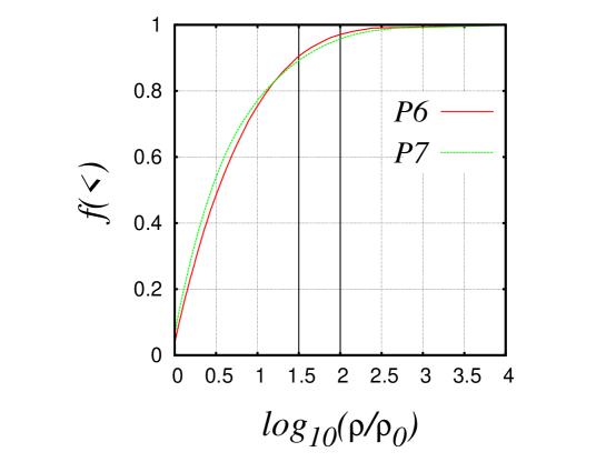
Figure 1: The fraction of the number of cubic elements having a ratio of the normalized density with a value less than the value of the horizontal axis. The vertical lines at 1.5 and 2 determine the density threshold of the chosen cubic elements, as defined in the text, see Section 2.3.

Some of the properties of these sets of chosen cubic elements of the partitions are shown in Table 1, as follows: column one shows the label of each partition; column two shows the partition level defined above and the number of identical cubic elements; column three shows the minimum density value used to define the set of chosen cubic elements; column four shows the number of chosen cubic elements per each partition; column five shows the number of cubic elements that are linked as neighbors, see Section 3.3 below and column six shows the peak number of gas particles found in only one cubic element of this set of chosen cubic elements.

It should be mentioned that the number of particles inside each cubic element can also be used as the selection criterion to define the chosen cubic elements. In this case, there would be a minimum particle number given before-hand, so that only those cubic elements with a greater number of particles would be considered in the calculation of properties. However, the results are more interesting when the criterion is based on density. In Fig. 2 we show the distribution function of the number of cubic elements against the number of gas particles inside each cubic element.

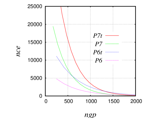
Figure 2: The distribution function of the number of gas particles (shown in the horizontal axis) inside each chosen cubic element (shown in the vertical axis).

The spatial distribution of the identical cubic elements defined in this section is shown Figs. 3 and 4, in which the normalized density value appears in the right-hand column of each plot as ${\rm lrho0}$.

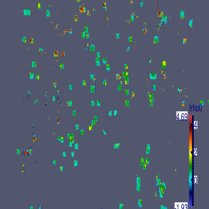
Figure 3: Spatial distribution of all the cubic elements satisfying the density condition defined in Section 2.3 using partition P6. The length of the side is 100 Mpc.

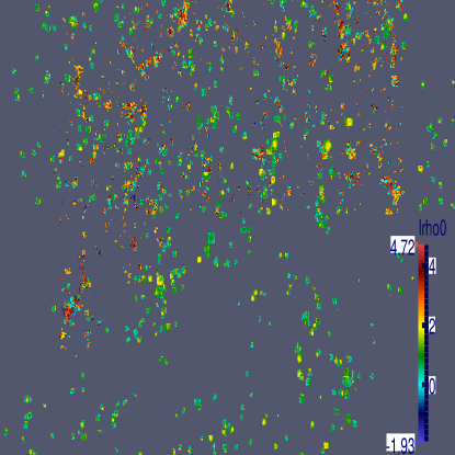
Figure 4: Spatial distribution of all the cubic elements satisfying the density condition defined in Section 2.3 using the partition P7. The length of the side is 100 Mpc.

3 Results

To highlight the spatial scale of the simulation and the code presented in this paper, let us now summarize, very briefly, the well-established current scenario about the formation of structure in cosmological simulations. At the scale of 100 Mpc and redshift z=0, our simulations will produce a cosmic network of dense filaments. At a scale of 10 Mpc, the most massive dark-matter halos will be formed mainly at the intersection of those filaments. At a scale of a few Mpc, the gas will condense and start forming virialized regions in the center of the collapsed dark-matter halos, so that galaxy clusters will appear. At a scale of a few kpc, the dense gas will form galaxies, so that at the nucleus of some of the galaxies, at the scale of a few pc, the gas will collapse gravitationally to start forming stars.

In Sections 3.1-3.3, we will characterize the set of chosen cubic elements defined in Section 2.3. The gas particles contained in these chosen cubic elements of the partitions will be considered as an approximation of the distribution of the gas clumps, as is explained in Sections 3.4 and 3.5. It will be seen that an approximate size of these gas clumps is of the order of 1 Mpc or less, while the groups formed by these gas clumps are of the order of a few Mpc, and can therefore be identified with the structures forming virialized regions of gas (as mentioned in the previous paragraph).

3.1 The distribution function of the mass for the chosen cubic elements

We first count the gas particles within each chosen cubic element of the partition and thus immediately have the mass contained. We determine the minimum and maximum masses of this set of gas particles and make a mass partition in terms of $n_{\rm bin}=50$ bins, so that we count all the chosen cubic elements with a mass within each mass bin. The resulting distribution function of the mass of the chosen cubic elements is shown in the top panel of Fig.5.

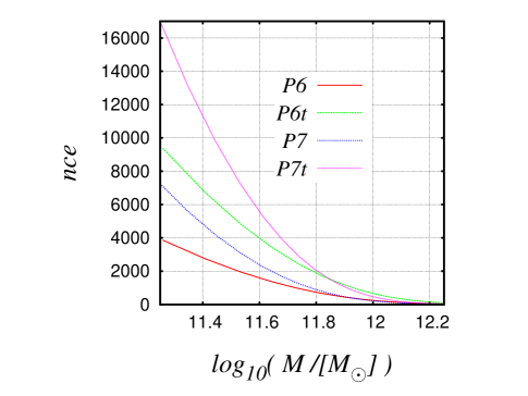
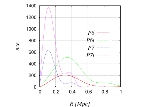
Figure 5: (top) The mass distribution function for the chosen cubic elements of the partitions. The vertical axis shows the number of chosen cubic elements having a mass shown in the horizontal axis. (bottom) The size distribution function for the chosen cubic elements of the partitions. The vertical axis shows the number of chosen cubic elements having a radius shown in the horizontal axis.

The behavior of these curves are all similar, as expected: they are quite separated for the smallest mass scale, indicating that there is a large difference in the number of low-mass chosen elements found in each partition. The smallest mass scale identified for all the partitions is around $\log_{10}\left(M/M_{\odot}\right)\,\approx 11.2$, whereas the largest mass scale, according to column six of Table 1 is around 13, although the number of chosen cubic elements decreases significantly in the plot around a mass scale of 12.2.

It appears that the pair of curves for partitions P6-P7 and P6t-P7t are closer to each other. This indicates that for the mass determination, the resolution parameter of the partitions seems to be more important than the density threshold parameter.

3.2 The distribution function of the radius for the chosen cubic elements

Let us now estimate a distribution function of the size for the dense gas contained in each chosen cubic element. We again re-consider the gas particles determined in Section 3.1 to calculate the center of mass and then locate the particle that is furthest from this center of mass but still inside the chosen cubic element, so that half of this distance is defined as a geometrical measure of the set of gas particles contained in the cubic element. We next make a radial partition of the radii thus obtained in terms of $n_{\rm bin}=50$ radial bins, so that a distribution function can be obtained by this procedure, as shown in the bottom panel of Fig.5.

Let us emphasize that the radius of the horizontal axis in both panels of Fig. 5 is just a label to identify the shells of the radial partition. Let $rmax$ be the maximum distance of the furthest particle from the center of mass, as mentioned in the paragraph above. Then, for the grids P7 and P7t we have $rmax_{P7}$ and for the grids P6 and P6t we have $rmax_{P6}$. As expected, we always have $rmax_{P7}<rmax_{P6}$. This indicates that the grids P6 and P6t have radial shells with a width larger than the radial shells of the grids P7 and P7t. For this reason, the curves for the grids P6 and P6t are located to the right side of the curves for the grids P7 and P7t.

It should be noted that the partitions P6 have, in general, a core radius that is larger than those of the partitions P7, so that the average radius is around 0.3 and 0.1 Mpc, respectively. The fixed size of the cubic element of each partition, as explained in Section 2.3, determines an upper limit of the distribution function of the radius. However, the radii detected by this procedure are quite smaller than this upper limit.

It appears that the pair of curves for the partitions P6-P6t and P7-P7t are closer to each other. This indicates that for the size determination, the density threshold parameter of the partitions seems to be more important than the resolution parameter.

3.3 The distribution function of the multiplicity for the chosen cubic elements

To take further advantage of the partitions described in Section 2.3, we now determine the chosen cubic elements located in the same neighborhood. To do this, we first define a proximity parameter, which must be a distance. We start this calculation by arbitrarily using the hypotenuse of the cubic element of the partitions, as defined in Section 2.3, so that in the case of the partitions P6, this proximity parameter is fixed at 1.44; for the partitions P7 it is fixed at 2.88 Mpc.

We next determine all of the chosen cubic elements whose geometric centers are separated by a distance smaller than or equal to this proximity parameter. Let us define the multiplicity as the total number of cubic elements that are all linked to each other in this way, the result of this procedure is shown in Fig.6. Following this procedure, we have a list of neighbors for each chosen cubic element, which will be used again in Section 3.4.

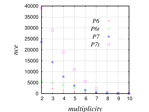
Figure 6: The multiplicity distribution function of the number of chosen cubic elements (shown in the vertical axis) having the number of neighbors (shown in the horizontal axis).

The case of groups with multiplicity 10 is remarkable, because many of these groups have been detected simultaneously with the same partition. For instance, the partition P6 detects five groups of multiplicity 10; 38 were detected with the partition P6t; only two were detected with the P7 and 13 were detected with the P7t. An example of such a highest multiplicity group is shown in Fig.7, where it can be noted that the gas clumps follow a filament. In addition, it should also be noted that the group shown in Fig.7 has been detected with both partitions P7 and P7t.

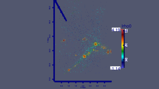
Figure 7: The group of chosen cubic elements with maximum multiplicity of 10 members, detected with both partitions P7 and P7t. Gas particles with a lower normalized density are allowed to enter in this plot to increase the total number of particles and improve the view.

Column five of Table 1 shows the total number of chosen cubic elements that are grouped in the some multiplicity level detected by this procedure. These numbers indicate that about 74 percent of the chosen cubic elements for partition P6 are placed into groups while 82 percent are placed in partition P6t. In the case of the partitions P7 and P7t, these fractions decreases to 65 percent and 74 percent, respectively.

Table 1: The partitions and some properties

partition label	partition level (nct)	lrhomin	nce	nceMult	ngpmax
P6	6 (643)	2.0	6795	5060	24801
P7	7 (1283)	2.0	50537	32891	17017
P6t	6 (643)	1.5	14408	11874	24801
P7t	7 (1283)	1.5	85810	64192	17107

3.4 Statistical properties of gas clump groups

To relate the gas particles contained in a chosen cubic element with a gas clump, in this section we impose two conditions on these gas particles so that they belong to a gas clumps if and only if: (i) the number of gas particles is greater than 10 and (ii) only gas particles with $\Phi_{i}<0$ will be considered to be in a gas clump.

To begin with the characterization of the gas clumps and their grouping properties, we first re-consider the list of neighbors obtained in Section 3.3. In addition, the proximity parameters for all the partitions are the same as those that were used in Section 3.3.

The application of these conditions on the list of neighbors has the immediate result that the number of groups per multiplicity decreases significantly, as can be seen in Fig.8, which must be compared to Fig.6. In addition, the groups of multiplicity 10 are no longer detected for any of the partitions. Consequently, in the x-axis of Fig.8, a multiplicity number is shown if and only if a non-zero number of groups is detected.

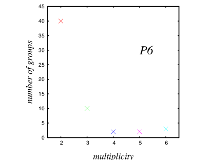
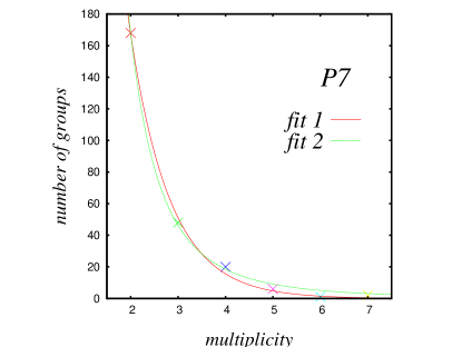
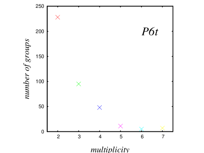
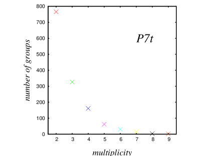
Figure 8: The number of groups (ng) detected are shown in the y-axis (using the point symbol x) in terms of the multiplicity (m) shown in the x-axis. Two lines are included in the top-right panel to fit the data with the following formulae: $ng1(m)=I_{1}*\exp(-m/ms)$ (fit 1) and $ng2(x)=I_{2}*(x/ms_{2})^{-n_{2}}$ (fit 2). The values of the fitting parameters are $I_{1}=1802.23$, $m_{s}=0.841847$, $I_{2}=17.1243$, $n_{2}=3.18728$ and $m_{s2}=4.09685$.

By only taking into account the groups of gas clumps detected after these conditions, we now calculate their average physical properties in terms of both their multiplicity and the partition in which they were found. The average mass resulting of the groups is shown in Fig.9. According to Section 2, the gas particles of the simulation have all the same mass, as given by $m_{p}\approx 6.4\times 10^{8}M_{\odot}$, so that the plots of Fig.9 also contain information about the average number of gas particles per group of a given multiplicity.

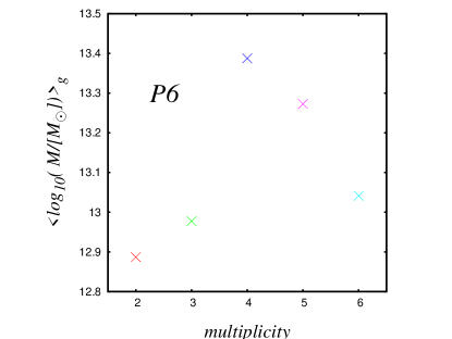
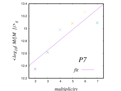
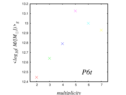
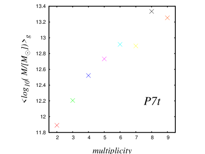
Figure 9: The average mass of the groups detected in terms of the multiplicity shown in the x-axis. A line is included in the top-right panel to fit the data with the following formula: $lm_{f}(x)=lm_{a_{1}}*(x/m_{s})+lm_{a_{0}}$. The values of the fitting parameters are $lm_{a_{1}}=0.29483$, $lm_{a_{0}}=12.1551$ and $m_{s}=1.78779$.

The panels of Fig.9 seem to indicate that the mass of a middle multiplicity group is always larger than the mass of the highest multiplicity group detected.

The average radius per group is shown in Fig.10. It should be emphasized that this radius makes sense only in geometrical terms. To obtain this radius, we first calculate the center of mass of the set of gas particles per each group. Then, we determine the gas particle furthest away from this point and take half of this distance as the radius per each group. Next, we calculate the average of all these radii and we show the result in terms of the group multiplicity. The panels of Fig.10 indicate that the radius of a lower multiplicity group is larger than the radius of the highest multiplicity group detected.

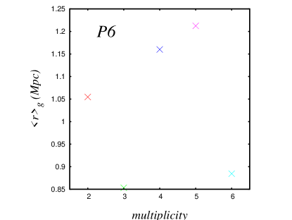
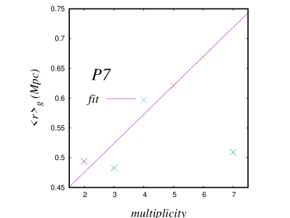
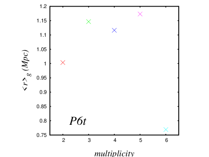
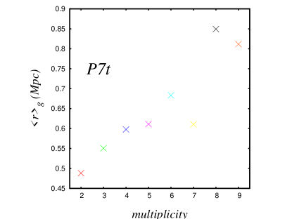
Figure 10: The average radius of the groups detected with the multiplicity shown in the x-axis. A line is included in the top-right panel to fit the data with the following formula: $rad_{f}(x)=rad_{1}*(x/m_{s})+rada_{0}$. The values of the fitting parameters are $rad_{1}=0.0795668$, $rad_{0}=0.37783$ and $m_{s}=1.63$.

Finally, the average velocity dispersion of the groups detected is shown in Fig.11. We emphasize that this velocity dispersion is calculated in the usual statistical sense: we calculate the magnitude of the velocity vector for all the gas particles of a given group, we then obtain the average velocity of all the groups and the dispersion is determined as the standard deviation, so that it is the square root of the variance; see [Press et al. (1992)]. The results are shown in terms of the multiplicity number.

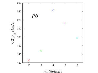
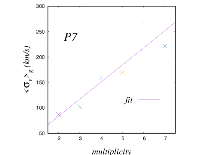
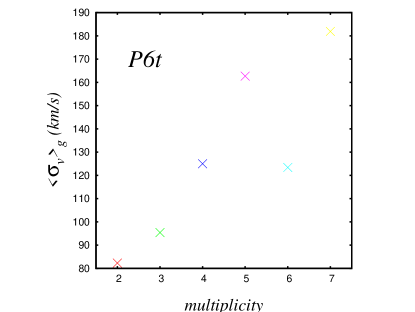
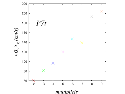
Figure 11: The average velocity dispersion of the groups detected in terms of the multiplicity shown in the x-axis. A line is included in the top-right panel to fit the data with the following formula: $\sigma_{f}(x)=\sigma_{1}*(x/m_{s})+\sigma_{0}$. The values of the fitting parameters are $\sigma_{1}=1.47406$, $\sigma_{0}=16.326$ and $m_{s}=0.0437996$.

It should be emphasized the use of the symbol $<>_{g}$ (in the vertical axis of all of the figures described up to this point) indicates that the physical properties are calculated using all of the gas particles associated to all of the detected groups. However, to complement Table 1, we now consider all the gas particles of a given multiplicity but this time irrespective of the particular group to which they belong. The total number of gas particles detected in terms of their multiplicity is shown in Fig.12.

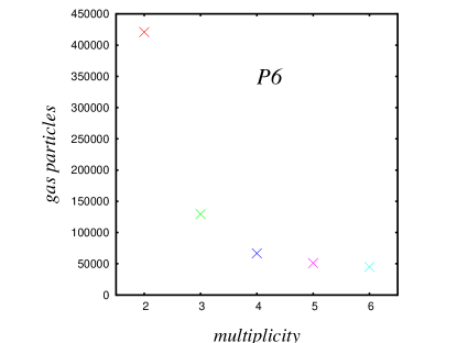
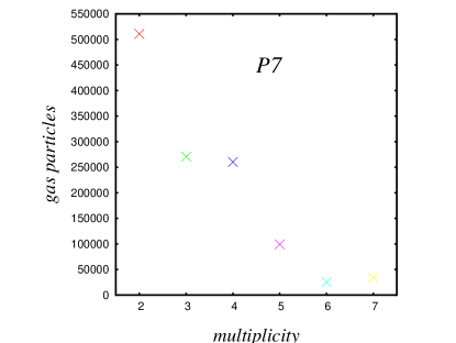
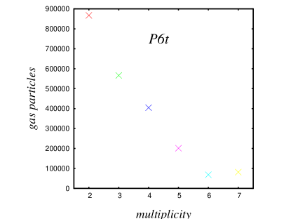
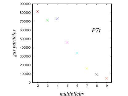
Figure 12: The total number of gas particles found in any group with the multiplicity shown in the x-axis.

To take advantage of these results, we now summarize in Table 2, the fitting curves for all of the physical properties of the galaxy groups, that is, those indicated previously by the symbol $<>_{g}$.

A measure of the variation of the fitted data can be obtained by calculating the sum of squares of residuals, denoted here by $SS$, so that a standard error can be defined by $SE=\sqrt{SS/dF}$, where $dF$ is the number of degrees of freedom, which is defined as the number of fitted points minus the number of fitting parameters. The goodness of a fit can be established by introducing the variance of residuals (or reduced $\chi_{\nu}^{2}$), which is given by $SE^{2}$. These values are reported in the last column of Table 2 for each fitting formula. In principle, a value of $\chi_{\nu}^{2}$ around 1 indicates a good fit; a value of $\chi_{\nu}^{2}\gg 1$ indicates a poor model fit; finally, a value of $\chi_{\nu}^{2}<1$ indicates that there is noise in the model fit, which is usually named as ”over-fitting” the data.

The goodness of the fitting parameters can be established by a confidence interval, which is determined by the best value of a fitting parameter $\pm\;tS*SE$, where $tS$ is the value from the $t$-distribution for the specified number of degrees of freedom and with 95 percent of confidence. In Table 3 we show these confidence intervals, so that the order of the fitting formulae shown in Table 2 is still followed in Table 3.

Finally, by calculating the mean $x_{\rm ave}$ and standard deviation $SD$ of the data array $x$, with $n_{p}=6$ points in this case, which are plotted in the vertical axis of each of the top right panels of Figures 8-11, a confidence interval of the physical properties can be determined by the equation $x_{\rm left}=x_{\rm ave}-tS*SD/\sqrt{n_{p}}$ for the left side and by the equation $x_{\rm right}=x_{\rm ave}+tS*SD/\sqrt{n_{p}}$ for the right side, so that these values are reported in columns 4 and 5 of Table 4.

In order to quantify the influence that the use of the grid P6 can have on the results, in Table 5 we repeat only the calculation described in the paragraph above, by using the physical properties plotted in the vertical axis of each of the top left panels of Figures 8-11.

Table 2: Fitting formulae of the mean physical properties of groups in terms of their multiplicity (m)

symbol	fitting formula	Figure	variance of residuals $\chi_{\nu}^{2}$
$N_{g}(m)$	$1802.23\times\exp\left(-m/0.841847\right)$	Fig.8	8.37
$N_{g}(m)$	$17.1243\times\left(m/4.09685\right)^{-3.18728}$	Fig.8	10.94
$<\log\left(M/M_{\odot}\right)>(m)$	$0.29483\times(m/1.78779)+12.1551$	Fig.9	0.04
$<r>(m)$	$0.0795668\times(m/1.63)+0.37783$	Fig.10	0.001
$<\sigma_{v}>(m)$	$1.47406\times(m/0.0437996)+16.326$	Fig.11	1253.93

Table 3: Confidence interval of the best value of the fitting parameter. The order of the fitting formulae shown in Table 2 is still followed here

symbol	best value	left side	right side
$I_{1}$	1802.23	1796.1	1808.4
$m_{s}$	0.841847	-5.3	7.0
$I_{2}$	17.12	9.3	24.9
$n_{2}$	3.2	-4.7	11.0
$m_{s2}$	4.09	-3.8	11.9
$lm_{a_{1}}$	0.29	-0.17	0.76
$lm_{a_{0}}$	12.16	11.67	12.62
$m_{s}$	1.79	1.32	2.26
$rad_{1}$	0.079	-0.026	0.18
$rad_{0}$	0.378	0.27	0.49
$m_{s}$	1.63	1.53	1.74
$\sigma_{1}$	1.47	-81.84	84.79
$\sigma_{0}$	16.326	-67.0	99.6
$m_{s}$	0.0437996	-83.3	83.3

Table 4: Confidence interval of the physical properties by using the grid partition P7

Label	mean	standard deviation	left side	right side
$N_{g}$	40.8	59.11	-6.47	88.13
$<\log\left(M/M_{\odot}\right)>$	12.9	0.31	12.65	13.15
$<r>(Mpc)$	0.56	0.07	0.50	0.62
$<\sigma_{v}>(Km/s)$	167.78	62.69	117.60	217.94

Table 5: Confidence interval of the physical properties by using the grid partition P6

Label	mean	standard deviation	left side	right side
$N_{g}$	11.4	14.61	-1.77	24.57
$<\log\left(M/M_{\odot}\right)>$	13.11	0.19	12.9	13.23
$<r>(Mpc)$	1.03	0.14	0.90	1.16
$<\sigma_{v}>(Km/s)$	181.5	42.26	143.42	219.58

3.5 The distribution function of the ratio $\frac{E_{\rm kin}}{\left|E_{\rm grav}\right|}$ of the gas clumps

We now continue the characterization of the dense gas clumps contained in the chosen cubic elements by calculating their ratio of the kinetic energy to the gravitational energy. The energies involved are:

$$\begin{array}[]{l}E_{\rm ther}=\frac{3}{2}\sum_{i}\,m_{i}\frac{P_{i}}{\rho_{i}}\\ E_{\rm kin}=\frac{1}{2}\sum_{i}\,m_{i}v_{i}^{2},\\ E_{\rm grav}=\frac{1}{2}\sum_{i}\,m_{i}\Phi_{i}\end{array}$$ (1)

where the summations include all of the gas particles inside each chosen cubic element, so that $\Phi_{i}$ is the gravitational potential, $v_{i}$ is the velocity, $m_{i}$ is the mass and $P_{i}$ is the pressure.

In simulations of the gravitational collapse of clouds, the dynamic behavior is mainly determined by the values of the ratio of the thermal energy to the potential energy, $\frac{E_{\rm ther}}{\left|E_{\rm grav}\right|}$, and the ratio of the kinetic energy to the gravitational energy, $\frac{E_{\rm kin}}{\left|E_{\rm grav}\right|}$; see [Miyama et al. (1984)]. In addition, these ratios are very important to determine the stability of a gas structure against gravitational collapse, so that collapse and even fragmentation criteria can be constructed in terms of these ratios; see [Hachisu and Heriguchi (1984)], [Hachisu and Heriguchi (1985)] and the references therein. These ratios also characterize very well the gravitational collapse by capturing the most representative events, including fragmentation, which may leave an imprint on the value of these ratios; see [Arreaga-Garcia and Saucedo (2012)].

It must be mentioned that most of the codes considered in [Knebe et al. (2011)] apply a procedure to improve the list of particles that potentially belong to a halo. We did not implement a complete procedure to remove unbound gas particles. However, only gas particles with $\Phi_{i}<0$ have been considered in the calculation of this Section 3.5, because these particles are gravitationally linked. Once these particles are selected in each chosen cubic element, we then calculate the ratios defined in this section. It is important to emphasize that only those chosen cubic elements with a number of particles greater than 200 are considered in this calculation.

We consider it to be more illustrative to present the results of this calculation in terms of the number of cubic elements, $nce$ found within a given interval of the ratio $\frac{E_{\rm kin}}{\left|E_{\rm grav}\right|}$, as has been done in previous sections the result is shown in Fig. 13.

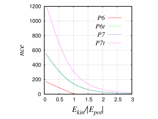
Figure 13: The distribution functions of the number of chosen cubic elements $nce$ (shown in the vertical axis) against their ratio of kinetic energy to gravitational energy (shown in the horizontal axis).

The curves thus obtained indicate that most of the chosen cubic elements have low-values of the ratio $\frac{E_{\rm kin}}{\left|E_{\rm grav}\right|}$, so that most of the gas inside each chosen cubic element is clustered such that its average value is $\frac{E_{\rm kin}}{\left|E_{\rm grav}\right|}<1$.

4 Discussion

In this paper we applied a mesh-based code to generate a uniform cubic partition to characterize the clustering and grouping properties of gas clumps at galaxy cluster scales using a typical cosmological simulation.

It must be first emphasized that the results reported in Sections 3 depend strongly on the parameters of the partition, as expected. This is a common situation, even in highly-refined codes presented elsewhere, in which the main parameters of the code must be given before-hand. Here, we will consider other features to clarify the results obtained and their dependence on the partition used. The basic partition depends on two parameters, namely: the level of resolution and the density threshold. The low-resolution partitions were labeled as P6 and P6t, corresponding to a density threshold of 2 and 1.5, respectively; analogously, the high-resolution partitions were labeled as P7 and P7t, respectively.

A high fraction of the chosen cubic elements contained more than 500 particles, as can be seen in Fig.2, so that the gas clumps are expected to be well represented in this low-resolution simulation. However, the edges of the chosen cubic elements of partition P6 and P6t were visible in Fig. 3. This indicates that the size of their typical cell element was too big, and there can be more than one gas clump contained in each cell element. Fortunately, the edges were less visible in the partitions P7 and P7t, as can be seen in Fig. 4. This indicates that only the core of the largest gas clumps were captured by each cell element. These features can be seen as shortcomings of this method. On the other hand, a positive feature of this method is that it can certainly be identified filamentary distributions of cubic elements. Nevertheless, by comparing the distributions of cubic elements seen in Figs. 3 and 4, one then can see the critical role played by the normalized density threshold: the higher its value, the better its representation of the gas clumps by the set of chosen cubic elements.

A large number of chosen cubic elements were linked in lower-multiplicity groups. Specifically, in the case of multiplicity 2, the ratio of these numbers between the partitions P7 to P6 is around 8. This means that there are 8 times more binary systems of the chosen cubic elements in partitions P7 than those detected in partition P6. A similar ratio was observed in the case of partitions P7t to P6t; see Fig.6. This behavior indicates that a change in the resolution has a significant impact. Meanwhile, a small change in the density threshold does not affect too much the larger number of the chosen cubic elements detected in partitions P7 and P7t as compared with those obtained for partitions P6 and P6t.

However, analogous ratios constructed with the number chosen cubic elements of multiplicity 2 between the partition P7t to P7 and P6t to P6 indicate that the change is smaller than that observed in the previous paragraph, so that it is now about 1.6. This means that the number of binary systems of chosen cubic elements does not duplicate when we change the density threshold from 2 to 1.5 in partitions with the same level of resolution.

As noted in Section 3.4, after imposing the two conditions on the gas particles contained in the chosen cubic elements, the number of groups detected in terms of their multiplicity decreased significantly. Let us consider again the case of multiplicity 2 that was discussed above, then the ratio between the numbers of groups detected in the partitions P7 to P6 and P7t to P6t are now of the order 4. This means that now there are 4 times more binary systems of gas clumps in the partitions of level 7 than those detected in the partitions of level 6. Surprisingly, a comparison of the analogous ratios between the partitions P7t to P7 and P6t to P6 indicate that they are of the same order 4.

The numbers of interest detected for partitions P6t and P7t almost doubled when compared to those detected for the original partitions P6 and P7 ( e.g. the number of chosen cubic elements, the number of groups, etc.) Meanwhile, the physical properties of the groups are comparable; for instance, the mass scale in terms of $\log_{10}\left(M/M_{\odot}\right)$ for partition P6 ranges within 12.9–13.4; while for partition P6t, it ranges within 12.4–13.1; for the partitions P7 and P7t we observed the normalized mass range within 12.3–13.3 and 11.8–13.4, respectively.

Apparently, it will be easier to lose the gas clumps originally detected when the multiplicity of the associations of chosen cubic elements is higher. It is very likely that the gas clumps associated in higher-multiplicity groups are too small and do not meet the conditions imposed in Section 3.4. It is also possible that the highest-multiplicity groups still detected in Section 3.4 are incomplete in their number of members in view of this behavior.

While it is true that only gravitationally bounded gas particles were used to identify gas clumps and determine group properties in Section 3.4, it must be noted that no test was made to check whether the gas clumps that were placed in groups are gravitationally bound to each other. In addition, the proximity parameter introduced in Section 3.3 was motivated by the size of the cubic element of the partitions, which means that it can be changed and the results are going to be changed accordingly.

However, a proximity parameter can in principle be found, so that its cubic partition be the better choice for a given simulation. In fact, N-body simulations and the friends-of-friends algorithm have been used to calibrate these kind of codes to obtain values of linking length parameter, so that it makes the best identification of galaxy groups in catalogs; see for instance [Eke et al. (2003)], [Padilla et al.(2004)] and [Norberg et al. (2003)].

In Section 3.5 we calculated the ratio of kinetic energy to gravitational energy of all the gas clumps contained in the chosen cubic elements. These values can be useful as initial conditions for simulations of the formation of star clusters, like the ones simulated by [Klessen and Burkert (2000)] and [Klessen and Burkert (2001)]. However, the physical properties of the gas cloud progenitors that will produce the star clusters by gravitational collapse, are difficult to obtain, mostly because these cluster precursors are very difficult to be observed. Nevertheless, [Jackson et al. (2018)] have recently observed ”a high mass molecular cloud with unusually large linewidths”, which indicate that its level of kinetic energy is so high, that this cloud was difficult to be considered as a gravitationally bound system. These authors claimed that if this system were successfully identified as a star cluster progenitor, then this cloud must be dominated by extreme turbulence. It has been shown elsewhere that this kind of highly turbulent cloud can still collapse and form protostars, see [Arreaga-Garcia (2018)].

5 Comparison with other papers and observations

A natural way to assess the results reported in this paper is by means of a comparison with other simulations. In spite of the fact that our gas structures are just a crude representation of the real distribution of galaxies, we will also try to make a comparison with observations. In order to keep these comparisons tractable, in this Section we will focus only on the results obtained by using the partition P7t, which has given us the best results.

With regard to the numerical simulations side, there is a rich literature on multiplicity functions in cosmology that can be mentioned. For instance, using early dark-matter only simulatons, [Gott and Turner (1977)] described the clustering of galaxies in terms of a multiplicity function, defined as the fraction of galaxies in single, double, triple systems, etc. [Bhavsar et al. (1981)] determined the number of groups in terms of the number of galaxy members. [Efstathiou et al. (1988)] compared the multiplicity function obtained from N-body simulations with the Press and Schechter formalism, which presented an approximate theory for the form of the multiplicity function, see [Press and Schechter (1974)]. A mathematical definition of multiplicity is given by [Efstathiou et al. (1988)], which is ”the multiplicity of each particle is $m$ if it is part of a group with more than 2^m-1 but no more than 2^m members”.

The ratio of the number of galaxies forming groups with 2 or 3 members between the number galaxies in groups of 4 or 5 members is 4 according to [Bhavsar et al. (1981)] and 8 according to [Efstathiou et al. (1988)]. According with our plots shown in the right column of Fig.8, our ratio is around 8.

[Thomas and Couchman (1992)] presented simulations on the formation of a rich cluster of galaxies, in which many small galaxies are detected in the region around the central galaxy by using a minimum density cut of 180 times the mean density of the simulation, so that 12 gas clumps are located the outer region beyond 1 Mpc and 20 gas clumps within this radius. Figure 11 of [Thomas and Couchman (1992)], presented a projection to the X-Y plane of the particle distribution, it shows a galaxy distribution very similar to that shown here in Fig.7.

In addition, in the paper [Perez et al. (2006a)], the authors located the gravitational bounded gas structures of a cosmological hydrodynamical simulation by using the friends-of-friends algorithm, see [Davis and Peebles (1985)]. Then, they continued by looking for condensed gas substructures within regions of 0.5 Mpc, centered on each bounded system localized, so that they identified a galaxy-like object with those gas concentrations found as substructure. They found 364 systems in pairs. After applying a proximity criterion, they finally obtained 88 galaxies-like objects in pairs. From these sample they constructed a 3D catalog and made an statistical analisys. This method goes beyond the capabilities of the code presented in this paper, which does not allow to capture gas substructures, so that a comparison is dificult to make. However, their number of galaxies in pairs seems to be quite small as compared with the more than 700 binary systems we found by using the partition P7t.

[Sales et al. (2007a)] found an average of about 10 satellite galaxies within the virial radius by using a friends-of-friends algorithm on a hydrodynamical simulation of a small region, which was taken from a cosmological simulation box and then re-simulated with the zoom-in technique, that is, at higher resolution but preserving the tidal fields from the whole box. It is interesting to mention that in this paper, groups of gas clumps up to 10 members were studied, because groups with a larger number of members were no found.

With regard to the observational side, it must be emphasized that catalogs of galaxies and cluster of galaxies have been generated from the data published by the 2dF Galaxy Redshif Survey, see for example [Tago et al. (2005)] and [Tago et al. (2006)]. The final release of the 2dFGRS contained 245591 galaxies out of which all group of galaxies catalogues were constructed using selection criteria and a cluster-finding method based on the well-known friends-of-friends algorithm, see [Davis and Peebles (1985)]. [Tago et al. (2005)] identified 7657 and 10058 groups of galaxies in the Northern (N) and Sourthern (S) parts of the 2dF GRS, respectively.

These numbers are quite large compared with the numbers reported in this paper, because we obtained 1363 groups of gas clumps in the P7t cubic partition, see the right bottom panel of Fig.8. Nevertheless, some physical properties obtained here are similar to those reported by [Tago et al. (2005)]. For instance, the size of most of the groups of galaxies detected by [Tago et al. (2005)] is within 0.1-0.5 h${}^{-1}\,$Mpc ( see the left panel of their Fig. 3). Meanwhile, the average effective radius of groups of galaxies found by [Tago et al. (2006)] is 0.61 h${}^{-1}\,$Mpc. In this paper, we obtained an average group radius in the range of 0.5-0.8 Mpc, as can be seen in the right bottom panel of Fig.10. The dispersion of velocity found by [Tago et al. (2005)] is similar for both the N and S parts of the 2dF GRS, around 200 km/s for groups of galaxies with less than 10 members ( see the left panel of their Fig. 4). In this paper, we obtained an average dispersion of velocity within the range of 80 to 200 km/s, as can be seen in the right bottom panel of Fig.11.

The mass of the groups of galaxies can be estimated by using the virial theorem and a typical size and velocity dispersion. For groups with three or a very few more member galaxies, this dynamical mass is within the range 10^12.5 to 10¹⁴ M_⊙, see [Geller M. J. and Huchra (1983)], [Nolthenius et al. (1987)], [Eke et al. (2004)], [Berlind et al. (2006)], [Yang et al. (2005)] and [Yang et al. (2007)]. In addition, by using a large set of galaxies contained in the fourth data release of the SDSS-DR4, see [Adelman-McCarthy et al. (2006)], [Zandivarez et al. (2006)] cataloged groups of galaxies, whose relationship between environment and physical properties was studied by [Martinez and Muriel (1998)]. In the bottom right-hand panel of Fig.1, [Martinez and Muriel (1998)] reported the log of the mass distribution of the groups sample against the number of groups with more than four members. They found that most of the groups have a log(M) around 13, so that it is in good agreement with tha mass reported in the right-hand panels of our Fig.9 for gas groups of multiplicity 4.

6 Concluding Remarks

Some galaxy surveys, as the Euclid Space Mision ( see [Laureijs et al. (2011)] ), the Sloan Digital Sky Survey ( see [York et al. (2000)] ), the Plank Survey ( see [Planck (2005)], [Planck (2014)] and [Planck (2016)]) , among others, will deliver new data shortly, so that the properties of galaxy clustering and galaxy groups will continue to be probes to study the growth of large scale structure of the Universe. For this reason, the development of algorithms to detect groups and cluster of galaxies is always needed.

With this purpose in mind, in this paper several uniform cubic partitions of the simulation volume were implemented to detect isolated dense gas clumps and calculate their clustering and grouping properties at galaxy cluster scales in a typical cosmological simulation.

Throughout Sections 3.1 to 3.4, and particularly in the first paragraphs of Section 4, we demonstrated that the low-resolution partitions P6 and P6t do not have enough resolution to describe the clustering and grouping properties considered, while the higher-resolution partitions P7 and P7t do a better representation. A higher level partition applied to a more resolved simulation will give better results at a much higher computational cost.

It is less conclusive is if there is any advantage when changing the normalized density threshold for a couple of partitions of the same resolution, such as P6 to P6t or P7 to P7t. We remark that partition P7t detected the largest multiplicity group of the simulation, even when compared to the partition P7.

In addition, we note that the highest multiplicity groups presented in section 3.4, do not generally have the largest size, mass and velocity dispersion when compared with lower multiplicity groups detected with the same partition. It can be expected that these physical properties of a group increase with respect to its multiplicity because more gas cloud members will need more space, will accumulate more mass and its further away particles will go faster.

Therefore, we conclude that our description of the grouping properties based on cubic partitions is partially acceptable because the low-multiplicity groups detected in this paper are in better agreement with these physical expectations.

In the simulation presented in this paper, the structures detected in small groups have a geometrical size within the range of 0.45–1.25 Mpc (mega-parsec); as discussed in Section 3.4. It is likely that most of the dense gas clumps forming these small groups will continue to collapse gravitationally, so that their size will diminish while their density will increase up to the point where galaxies be formed. It is therefore possible that the dynamics of the well-observed small groups of galaxies at kpc scale have been partially inherited from groups formed at a larger spatial scale of Mpc. The most important prediction of this work consists of the fitted curves that indicate how the physical properties of the groups will change in terms of the number of members or multiplicity, see Table 2.

To establish the goodness of the fitting models, the $\chi_{\nu}^{2}$ statistical test has been applied to the data. In principle, the two fits for the number of groups, $N_{g}$ and for the velocity dispersion $\sigma_{v}$ would qualify as poor fitting models; the fit for the log of the mass and the radius seem to be ”over-fitted”. For this reason, new fitting models need to be proposed.

To continue with the inspection of the certainty of the parameters of the fitting models, the confidence interval has been calculated and shown in Table 3. The confidence intervals are very wide in general, except for the fitting parameters of the log of the mass $<\log\left(M/M_{\odot}\right)>$ and the radius $<r>$.

To take advantage of all the physical information displayed at the vertical axis of Figures 8-11 and at the same time, to compare the results with the two sets of grids P7 and P6, to assess the influence of the grid on the study undertaken in this paper, in Tables 4 and 5 we showed the mean, the standard deviation and the confidence interval of each physical property.

By using the grid P6, a smaller number of low-multiplicity groups are detected, with a similar mass but with a slightly larger size and velocity dispersion in comparison with the properties obtained by using the grid P7. Being the log of the mass and radius the only physical properties which seem to be grid-independent, then these results would allow us to speak about the average physical properties expected for low-multiplicity groups of protogalaxies.

Thus, one can set forth the second prediction of this paper, which is that for low-multiplicity groups of protogalaxies, the average log of the mass is within the interval 12.65-13.23 and the average radius is within the interval 0.5-1.16 Mpc.

The third prediction in this paper is based on the calculation of the distribution of the chosen cubic elements in terms of their ratio values of $\frac{E_{\rm kin}}{\left|E_{\rm grav}\right|}$, which was shown in Fig.13. It should be emphasized that we found that most of the gas clumps have a low-value of $\frac{E_{\rm kin}}{\left|E_{\rm grav}\right|}$. This result is in agreement with observational estimates of the ratio $\frac{E_{\rm kin}}{\left|E_{\rm grav}\right|}$ in pre-stellar gas cores which are within the range 10^-4-0.07, see [Caselli et al. (2002)] and [Jijina (1999)].

Among the advantages of our method, the programming is easy and it leads in a natural way to the zoom-in technique, in which a cell of the partition can be chosen to re-simulate its content of matter and increase its number of particles to represent only that particular region in a new simulation box.

The zoom-in technique has allowed a single chosen galaxy or dark matter halo to be studied in great detail, see for instance [Roca-Fabrega et al. (2016)]. In our case, the results of this paper can be used as suitable initial conditions for numerical simulations that aim to follow the dynamical evolution of small groups of galaxies; for instance, [Barnes (1985)] and [Aceves and Velázquez (2002)] have started their simulations with a value of $\frac{E_{\rm kin}}{\left|E_{\rm grav}\right|}$ in the range 0.1–1.

7 acknowledgements

The author gratefully acknowledges the computer resources, technical expertise, and support provided by the Laboratorio Nacional de Supercómputo del Sureste de México through grant number O-2016/047.

References

- [Aceves and Velázquez (2002)] Aceves, H. and Velázquez, H., 2002, Revista Mexicana de Astronomía y Astrofísica, 38, pp.199-214.
- [Abadi (2009)] Abadi, M.G., 2009, Revista Mexicana de Astronomía y Astrofísica, 35, pp. 177-181.
- [Adelman-McCarthy et al. (2006)] Adelman-McCarthy J.K., et al, 2006, ApJS, 162,38.
- [Arreaga-Garcia (2016)] Arreaga-García, G., 2016, Revista Mexicana de Astronomía y Astrofísica, 52, 155-169.
- [Arreaga-Garcia (2017)] Arreaga-Garcia, G., 2017, Astrophysics and Space Science, 362. pp.47-69.
- [Arreaga-Garcia (2018)] Arreaga-Garcia, G., 2018, Astrophysics and Space Science, 363, Num.3, pp.12.
- [Arreaga-Garcia and Saucedo (2012)] Arreaga-García, G. and Saucedo-Morales, J.C., 2012, Revista Mexicana de Astronomía y Astrofísica, 48, pp. 61-84.
- [Balsara (1995)] Balsara, D., 1995, J. Comput. Phys. 121, 357.
- [Barnes (1985)] Barnes, J.E., 1985, MNRAS, 215, 517.
- [Berlind et al. (2006)] Berlind A. A., Frieman J., Weinberg D. H., et al. 2006, ApJS, 167, 1.
- [Bate et al. (2003)] Bate, M. et al., 2003, MNRAS,339, 577.
- [Bate and Burkert (1997)] Bate, M.R. and Burkert, A., 1997, MNRAS, 288, 1060.
- [Bergin and Tafalla (2007)] Bergin, E. and Tafalla, M. 2007, Annu. Rev. Astro. Astrophys., 45, 339
- [Bertschinger (1998)] Bertschinger, E., 1998, Annual Review of Astronomy and Astrophysics 36, 599–654.
- [Bhavsar et al. (1981)] Bhavsar,S.P., Gott III, J.R. and Aarseth,S.J., 1981, ApJ , 246, 656-665.
- [Birdsall and Fuses (1997)] Birdsall, C.K. and Fuss, D., 1997, Journal of Computational Physics, 135, pp. 141-148.
- [Bonnell, I. et al. (2001)] Bonnell, I. et al., 2001, MNRAS ,323, 785.
- [Caselli et al. (2002)] Caselli, P., Benson, P.J., Myers, P.C. and Tafalla, M., 2002, ApJ, 572, 238.
- [Cañas at. al. (2019)] Cañas, R., Elahi, P.J., Welker, C., Lagos, C. del P., Power, C., Dubois, Y. and Pichon, C., 2019, MNRAS, 482, pp.2039-2064.
- [Clark at. al. (2007)] Clark, P. et al., 2007, MNRAS ,379, 57.
- [N-GenIC (2003)] Web site: http://www.h-its.org/tap-software-en/ngenic-code/.
- [Davis and Peebles (1985)] Davis, M., Efstathiou, G., Frenk, C. S. and White, S., 1985, ApJ, 292, pp.371-394.
- [Dobbs and Pringle (2013)] Dobbs, C.L. and Pringle, J.E., 2013, MNRAS, 432, pp. 653–667.
- [Efstathiou et al. (1988)] Efstathiou, G., Frenk, C.S., White, S.D.M. and Davis, M., 1988, MNRAS,235, 715.
- [Eisenstein and Hut (1998)] Eisenstein, D.J. and Hut, P., 1994, ApJ, 498, pp. 137-142.
- [Eisenstein and Hu (1999)] Eisenstein, D.J. and Hu, W., 1999, ApJ, 511, 5.
- [Eke et al. (2003)] Eke, V. and the 2dFGRS team, 2003, Galaxy evolution in groups and clusters, A jenam workshop, Edited by Catarina Lobo and Margarita Serote Roos and Andrea Biviano, Astrophysics and Space Science, v. 285, pp. 205-209.
- [Eke et al. (2004)] Eke V. R., Baugh C. M., Cole S., et al. 2004, MNRAS, 348, 866-.
- [Gill et al. (2004)] Gill, S.P.D., Knebe, A., and Gibson, B.K., 2004, MNRAS, 351, 399.
- [Geller M. J. and Huchra (1983)] Geller M. J. and Huchra J. P., 1983, ApJS, 52, 61-.
- [Gott and Turner (1977)] Gott III, J.R. and Turner, E.L.., 1977, ApJ , 216, 357-371.
- [Hachisu and Heriguchi (1984)] Hachisu, I. and Heriguchi, Y., 1984, Astron. Astrophys., 140, 259.
- [Hachisu and Heriguchi (1985)] Hachisu, I. and Heriguchi, Y., 1985, Astron. Astrophys., 143, 355.
- [Hennebelle and Chabrier (2008a)] Hennebelle,P. and Chabrier,G., 2008, Astrophys. J.,684, 395.
- [Hennebelle and Chabrier (2008b)] Hennebelle,P. and Chabrier,G., 2008, Astrophys. J.,702, 1428.
- [Hickson (1982)] Hickson, P., 1982, ApJ, 255, 382-391.
- [Hopkins (1012)] Hopkins, 2012, MNRAS, 423, 2037.
- [Jackson et al. (2018)] Jackson, J.M., Contreras, Y., Rathborne, J.M., Whitaker, J.S., Guzman, A., Stephenes, I.W., Sanhueza, P., Longmore, S., Zhang, Q. and Allingham, D., 2018, eprint arXiv:1811.06061.
- [Jijina (1999)] Jijina, J., Myers, P.C. and Adams, F.C., 1999, ApJ, 125, pp. 161–236.
- [Kauffmann at al. (2013)] Kauffmann, J., Pillai, T. and Goldsmith, P.F.,2013, ApJ, 779, Issue 2,pp.14.
- [Kitsionas and Whitworth (2002)] Kitsionas, S., and Whitworth, A.P., 2002, MNRAS, 330(1), 129–136.
- [Klessen and Burkert (2000)] Klessen, R. and Burkert, A., 2000, ApJS, 128, pp.287-319.
- [Klessen and Burkert (2001)] Klessen, R. and Burkert, A., 2001, ApJ, 549, pp.386-401.
- [Klessen and Hennebelle (2010)] klessen, R.S. and Hennebelle, P., 2010, Astronomy and Astrophysics, Volume 520, id.A17, 18 pp.
- [Knebe et al. (2011)] Knebe, A., and 27 co-authors, 2011, MNRAS, 415(3), 2293–2318.
- [Knollmann et al. (2009)] Knollmann, S.R., and Knebe, A., 2009, ApJS 182, 608.
- [Laureijs et al. (2011)] Laureijs, R., Amiaux, J., Arduini, et al. 2011, Euclid Definition Study Report. arXiv e-prints.
- [L’Huillier et al. (2014)] L’Huillier, B., Park, C., and Kim, J., 2014, New Astronomy 30, 79–88.
- [Liu (2003)] Liu, G.R., 2003, Smoothed Particle Hydrodynamics, World Scientific Press.
- [Lombardi et al. (2010)] Lombardi, M., Lada, C. J. and Alves, J., 2010, Astronomy and Astrophysics, 512, A67.
- [Longair (1998)] Longair, M., 1998, Galaxy Formation, Springer-Verlag.
- [Mamon (1995)] Mamon, G.A., 1995, 3rd Chalonge Colloque Cosmologie, ed. H. de Vega and N. Sanchez (Singapore: World Scientific), meeting held in Paris, France, June 1995. arXiv:astro-ph/9511101.
- [Martinez and Muriel (1998)] Martinez, J.M. and Muriel, H., 2006, MNRAS, 370, 1003- 1007.
- [Miyama et al. (1984)] Miyama, S.M., Hayashi, C. and Narita, S., 1984, ApJ, 279, 621.
- [Monaghan and Lattanzio (1985)] Monaghan, J.J. and Lattanzio, J.C., 1985, Astronomy and Astrophysics, 149,p. 135-143.
- [Nolthenius et al. (1987)] Nolthenius R., White S. D. M., 1987, MNRAS, 225, 505-.
- [Norberg et al. (2003)] Norberg, P. and the 2dFGRS team, 2003, MNRAS, 336, 907.
- [Oey et al. (2011)] Oey, M.S., 2011, Astrophys. J. Lett.,739, L46.
- [Offner et al. (2014)] Offner, S.R., Paul C. Clark, P.C., Hennebelle, P., Bastian, N., Bate, M.R., Hopkins, P.F., Moraux, E. and Whitworth, A.P., Published in ”Protostars and Planets VI”, Eds. Henrik Beuther, Ralf S. Klessen, Cornelis P. Dullemond, and Thomas Henning (eds.), University of Arizona Press, Tucson, 2014, 914 pp., p.53-75. arXiv:1312.5326.
- [Owen and Villumsen (1997)] Owen, J.M. and Villumsen, J.V., 1997, ApJ, 481, pp.1-21.
- [Padilla et al.(2004)] Padilla, N. D.; Carlton B. M.; Eke, V. R.; Norberg, P.; Cole, S.; Frenk, C. S.; Croton, D. J.; Baldry, I. K.; Bland-Hawthorn, J.; Bridges, T.; Cannon, R.; Colless, M.; Collins, C.; Couch, W.; Dalton, G.; De Propris, R.; Driver, S. P.; Efstathiou, G.; Ellis, R. S.; Glazebrook, K.; Jackson, C.; Lahav, O.; Lewis, I.; Lumsden, S.; Maddox, S.; Madgwick, D.; Peacock, J. A.; Peterson, B. A.; Sutherland, W.; Taylor, K., 2004, MNRAS, 352, pp. 211-225.
- [Padoan and Nordlund (2002)] Padoan,P. and Nordlund,A., 2002, ApJ ,576, 870.
- [Paraview (2013)] Paraview, an open-source, multi-platform data analysis and visualization application, http://www.paraview.org/.
- [Pearce (1999)] Pearce, F.R., Jenkins, A., Frenk, C.S., Colberg, J.M., White, D.M., Thomas, P.A., Couchman, H.M.P., Peacock, J.A. and Efstathiou, G., 1999, ApJ, 521, pp.L99-L102
- [Perez et al. (2006a)] Perez, M.J., Tissera, P.B., Lambas D.G. and Scannapieco, C., 2006, Astronomy and Astrophysics, 449, pp.23-32.
- [Perez et al. (2006b)] Perez, M.J., Tissera, P.B. and Scannapieco, C., 2006, Astronomy and Astrophysics, 459, pp.361-369.
- [Planck (2005)] Planck Collaboration (2005). The Scientific Programme of Planck. ESA publication ESA- SCI(2005)/01.
- [Planck (2014)] Planck Collaboration, Ade, P.A.R., Aghanim, N. et al (2014). Planck 2013 results. XXIX. The Planck catalogue of Sunyaev-Zeldovich sources. Astronomy and Astrophysics, 571:A29.
- [Planck (2016)] Planck Collaboration, Ade, P.A.R., Aghanim, N. et al (2016). Planck 2015 results. XXVII. The second Planck catalogue of Sunyaev-Zeldovich sources. Astronomy and Astrophysics, 594:A27.
- [Planck (2013)] Planck Collaboration, Planck 2013 Results. XVI. Cosmological Parameters. arXiv:1303.5076.
- [Press and Schechter (1974)] Press, W.H. and Schechter, P., 1974, ApJ, 187,425.
- [Press et al. (1992)] Press, W.H., Teukolsky, S.A., Vetterling, W.T. and Flannery, B.P., 1992, Numerical Recipes in Fortran 77, Second Edition, Cambridge University Press.
- [Roca-Fabrega et al. (2016)] Roca-Fabrega, S., Valenzuela, O., Colin, P., Figueras, F., Krongold, Y. and Velazquez, H., 2016, ApJ, 824. ArXiv e-prints 1504.06261v2.
- [Sales et al. (2007a)] Sales, L.V., Navarro, J.F., Abadi, M.G. and Steinmetz, M., 2007a, MNRAS, 379, pp.1464-1474.
- [Sales et al. (2007b)] Sales, L.V., Navarro, J.F., Abadi, M.G. and Steinmetz, M., 2007b, MNRAS, 379, pp. 1475-1483.
- [Sawala et al. (2015)] Sawala, T., Frenk, C. S., Fattahi, A., Navarro, J. F., Bower, R. G., Crain, R. A., Dalla, V. C., Furlong, M., Jenkins, A., McCarthy, I. G., Qu, Y., Schaller, M., Schaye, J., and Theuns, T., 2015, MNRAS 448(3), 2941–2947.
- [Springel (2005)] Springel, V., 2005, MNRAS, 364, 1105.
- [Suginohara (1994)] Suginohara, T., (1994), Publications of the Astronomical Society of Japan, 46, pp.441-446.
- [Tago et al. (2005)] Tago, E., Einasto, J., Einasto,M. and Saar, E., (2005), Astronomy and Astrophysics manuscript, arXiv:astro-ph/0501099.
- [Tago et al. (2006)] Tago, E., Einasto, J., Saar, E., Einasto,M., Suhhonenko, I., Joeveer, M., Vennik, J., Heinamaki, P. and Tucker, D.L., (2006), Astron. Nachr., 327, pp.365-378.