Galaxy power spectrum and biasing results from the LOFAR Two-metre Sky Survey (first data release)

Abstract

The LOFAR Two-metre Sky Survey (LoTSS) is an ongoing survey aiming to observe the entire Northern sky, providing an excellent opportunity to study the distribution and evolution of the large-scale structure of the Universe. The source catalogue from the public LoTSS first data release (DR1) covers 1% of the sky, and shows correlated noise or fluctuations of the flux density calibration on few degree scales. We explore the LoTSS DR1 to understand the survey systematics and data quality of this first data release. We produce catalog mocks to estimate uncertainties, and measure the angular clustering statistics of LoTSS galaxies, which fit the $\Lambda$CDM cosmology reasonably well. We employ a Markov chain Monte Carlo (MCMC) based Bayesian analysis to recover the best galaxy biasing scheme and multi-component source fraction for LoTSS DR1 above $1$ mJy assuming different possible redshift templates. After masking some noisy and uneven patches and with suitable flux density cuts, the LOFAR survey appears qualified for large-scale cosmological studies. The upcoming data releases from LOFAR are expected to be deeper and wider, and will therefore provide improved cosmological measurements.

1. Introduction

Our present understanding of the origin and evolution of the Universe is based on the Lambda cold dark matter ($\Lambda$CDM) cosmology. In this model, the matter density of the Universe is dominated by cold dark matter, whose gravitational evolution results in a population of virialized dark matter halos of different masses (Press:1974; Scherrer:1991; Navarro:1997; Ma:2000; Seljak:2000; Scoccimarro:2001; Cooray:2002). The formation of galaxies occurs inside these dark matter halos, and the host halo mass and its evolution correlates with the evolution and type (Girelli:2020) of galaxy residing inside. In general, radio-loud galaxies’ active galactic nuclei (AGNs) are found to reside in more massive halos than optical AGNs (Mandelbaum:2008; Wilman:2008). That being so, the optical and radio observations sample quite a different set of galaxies (halos). Most galaxies which are bright at optical wavelengths are undetectable at radio wavelengths, and strong radio sources are often optically faint or invisible. The radio surveys sample the higher end of the halo mass range as compared with optical observations, and thus complement existing and upcoming visible/IR galaxy surveys (Kauffmann:2003; Best:2005; Mandelbaum:2009; Best:2014; Adi:2015nb; Krumpe:2018; Hale:2018; Alonso:2020jcy; Lan:2021; Wolf:2021).

The international Low-Frequency Array (LOFAR; Haarlem:2013) is a new-generation radio interferometer constructed in northern Netherlands and across Europe, offering increase in radio survey speed with unparalleled sensitivity and angular resolution in the low-frequency radio regime (Rottgering:2003; Haarlem:2005; Rottgering:2005; Falcke:2007). The LOFAR Two-metre Sky Survey (LoTSS) is an ongoing deep $120-168$ MHz imaging survey being carried out using LOFAR high-band antenna (HBA) observations across the whole northern hemisphere (Shimwell:2017; Shimwell:2019). The LoTSS aims to explore cosmic large-scale structure, galaxies, clusters of galaxies, and the formation and evolution of massive black holes. The LoTSS survey will observe millions of radio AGNs, along with a significant number of star-forming galaxies (SFGs) out to redshift $z\sim 6$, allowing detailed studies of the physics and evolution of AGNs and SFGs. The LoTSS is producing high-fidelity images at a central frequency of $144$ MHz with a resolution of $6\arcsec$ and with declination-dependent sensitivity, typically around $100\leavevmode\nobreak\ \mu{\rm Jy}$/beam. This is a factor of $10$ more sensitive than previous high-resolution sky surveys, e.g., VLA’s FIRST. LoTSS will ultimately detect over $10$ million radio sources with a significant fraction of star-forming galaxies. A large fraction of LoTSS sources will have optical identifications and photometric redshifts will be available (Williams:2019; Duncan:2019). Furthermore, the WHT Enhanced Area Velocity Explorer (WEAVE) multi-object spectrograph on the William Herschel Telescope will observe optical ($370-970$ nm) spectra of millions of LOFAR radio sources and provide precise redshift information (Smith:2016).

The LoTSS survey, homogeneously covering the whole northern sky complete down to the sub mJy limit will overcome statistical limitations due to shot noise. The large galaxy number density and large sky coverage will substantially reduce cosmic variance in cosmological analysis. The radio galaxies, tracing the background dark matter, will constrain the shape of power spectrum, i.e., the early universe physics, dark matter, baryon, and neutrino densities, the inflation power spectrum and the degree of non-Gaussianity in density fluctuations. The upcoming LoTSS catalogs, covering a large sky area, will help us to explore further regarding large-scale anomalies (Oliveira-Costa:2004; Ralston:2004; Schwarz:2004; Tiwari:2019l123) and the current puzzling dipole signal observed with radio catalogs (Blake:2002; Singal:2011; Gibelyou:2012; Rubart:2013; Tiwari:2014ni; Tiwari:2015np; Tiwari:2016adi; Colin:2017; Siewert:2020CRD). Furthermore, LoTSS will significantly improve on present low-frequency radio catalogs, e.g., TIFR GMRT Sky Survey (TGSS; Intema:2016tgss) and GaLactic and Extragalactic All-sky MWA (GLEAM; Hurley:2017gleam), and analyses based on these surveys (Tiwari:2016tgss; Rana:2019; Dolfi:2019; Tiwari:2019TGSS; Choudhuri:2020). Unfortunately, the link between the galaxy and total matter power spectra depends on some unknowns from astrophysics such as the galaxy bias factor, which depends on galaxy type and is quite different for radio AGNs and star-forming galaxies. The LoTSS population is a mixture of AGNs and star-forming galaxies, and therefore understanding galaxy bias, relative number densities and luminosity evolution is non-trivial. The purpose of this work is to present a detailed cosmological analysis of LoTSS galaxies and study the effect of survey footprint, shot-noise and other systematics. We have produced galaxy mocks for the survey and have customized and calibrated the data pipeline for galaxy clustering statistics recovery.

We introduce the catalog for LoTSS DR1, its completeness and data mask in Section 2 and 2.1. In Section 3, we present mock generation details and covariance matrix estimation. We briefly present the theoretical formulation of the galaxy angular power spectrum and its connection to the dark matter power spectrum in Section 4. In Sections 5 and 6, we present our measured angular power spectrum and two-point correlation statistics, respectively. We present an estimate for the bias for the LoTSS population in Section 7 and summarize our results in Section LABEL:sc:summary. We conclude with discussion in Section LABEL:sc:discussion.

2. LoTSS DR1 catalog

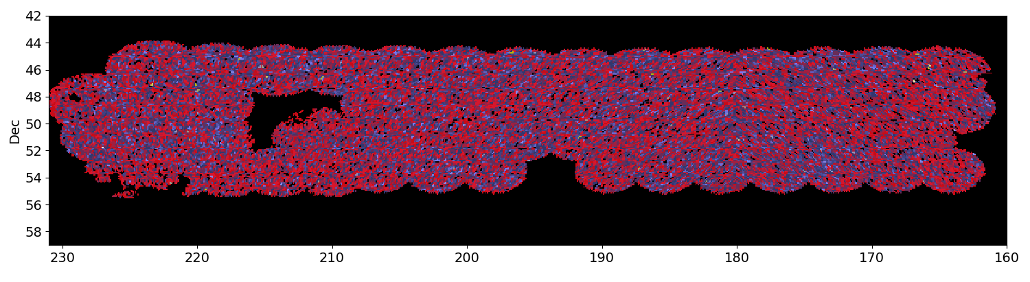
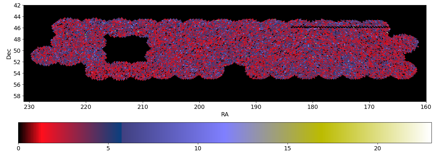
The LOFAR Two-metre Sky Survey (LoTSS; Shimwell:2017) is ongoing and plans to scan the entire northern sky at 120-168 MHz. Shimwell:2019 have prepared the first full-quality public data release (LoTSS-DR1) catalog from $63$ LoTSS data sets (2% of the total survey) in the region of the HETDEX Spring Field that were observed between 2014 May 23 and 2015 October 15. The LoTSS DR1 has been prepared using a fully automated direction-dependent calibration and imaging pipeline discussed in Shimwell:2017. The catalog covers $424$ square degrees and contains a total of $325,694$ sources with peak flux density at least five times the local rms noise, thus a source density of about $770$ sources per square degree. The resolution of the survey images is $6\arcsec$ and the positional accuracy of the sources in the catalog is within $0.2\arcsec$. The median sensitivity is $71\leavevmode\nobreak\ \mu{\rm Jy}$/beam at $144$ MHz. Williams:2019 remove artefacts, correct wrong groupings of Gaussian components and prepare a value-added catalog; the catalog then contains $318,520$ sources of which $231,716$ have optical/near-IR identifications in Pan-STARRS/WISE. Not all of these have photo-$z$ detection, as Pan-STARRS is not as complete as WISE and we only have photo-$z$s for about 50% of all radio sources.

Figure 1.— The distribution of radio galaxies in the LoTSS-DR1 catalog with integrated flux density between 1 to 10,000 mJy. Plotted are the number counts in pixels in Cartesian projection at HEALPix resolution Nside = 512 before (top) and after(bottom) applying the mask. After applying the mask and 1-10,000 mJy flux cut, there are 107926 sources remaining.

2.1. Completeness and data mask

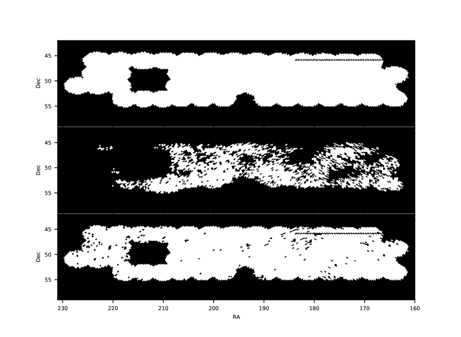
Shimwell:2019 estimate the completeness of LoTSS-DR1 and report the catalog to be $65\%$ complete at $0.23$ mJy, $90\%$ at $0.45$ mJy, and $95\%$ at $0.58$ mJy. The catalog is more than 99% complete at $1$ mJy. The LoTSS DR1 catalogue was generated by combining $58$ individual LOFAR pointings on the sky, and due to poor ionospheric conditions and due to the presence of bright sources, the imaging pipeline occasionally produces sub-standard images. As a result some pointings show inhomogeneous point source distribution, for example in particular 5 pointings show significant incompleteness (Siewert:2019). After properly defining the survey region and masking $5$ incomplete pointings, a reasonable survey mask (mask-z) for reliable cosmology is shown in figure 2. Mask-z is an upgrade to mask-d (Siewert:2019); it further rejects regions where information from Pan-STARRS is missing. In addition to mask-z we further consider masking cells with a local noise above the median noise (mask-z1) and two times the median noise (mask-z2). We impose the completeness flux cut (i.e., 1 mJy) and also remove the ultra bright sources with flux equal to or greater than $10$Jy; the catalog thus contains $121,730$ sources. After employing mask-z shown in figure 2, $107,926$ sources remain.

Figure 2.— LoTSS DR1 mask-z, z1 and z2. The mask-z (top) rejects 5 under-sampled pointings and includes all 53 good pointings of the LOFAR HETDEX field. Also it rejects regions of equal declination, where information from Pan-STARRS is missing. The mask has been prepared considering the survey geometry, consistency of source counts, and sampling uniformity (Siewert:2019). In the middle and bottom panel we show mask-z1 and mask-z2 which are obtained by further masking cells with a local noise above the median noise and two times the median noise, respectively.

3. Mock catalogs and Covariance matrix estimation

Mock catalogues are essential for assessing the analysis pipeline, data systematics and errors in the cosmological analysis of large galaxy surveys. In order to estimate the uncertainty in the cosmological signal recovered from LoTSS data, we generate $1000$ LoTSS mocks of the large-scale structure by employing the log-normal (and Gaussian) density field simulator code FLASK (Xavier:2016). To emulate the LoTSS DR1 catalog, we generate multiple log-normal density fields tomographically in $35$ redshift slices ($0$ to redshift $3.5$), each with a width $\Delta z=0.1$. All statistical properties (i.e., auto and cross-correlations) are determined by the input angular power spectrum. In addition, effects including redshift-space distortions and lensing are also included in the simulation via the input spectra provided to the FLASK pipeline.

The input theoretical angular power spectrum, $C_{\ell}$, in different redshift bins are generated using CAMB (Challinor:2011) which includes the effects on the observed number counts of redshift-space distortions, non-linear power spectrum corrections and lensing. The redshift distribution profile $N(z)$ is provided along with $C_{\ell}$ to FLASK to generate mock number count maps. Computation of theoretical $C_{\ell}$ requires a galaxy bias, $b(z)$. From our MCMC fits we iteratively provide best fitted bias and generate mock LoTSS DR1 catalogs. We assume a $\Lambda$CDM model and use Planck_results:2018 cosmological parameters as the fiducial cosmology throughout this work, in particular we set base cosmology parameters from Planck 2018 baseline, i.e. TT,TE,EE+lowE+lensing $\omega_{b}h^{2}=0.02237$, $\omega_{c}h^{2}=0.1200$, $100\theta_{MC}=1.04092$, $\tau=0.0544$, $\ln(10^{10}A_{s})=3.044$ and $n_{s}=0.9649$.

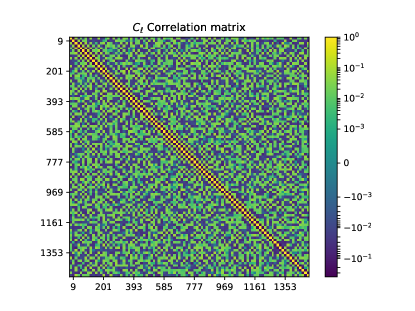
We apply the LoTSS DR1 survey mask to precisely account for survey geometry, then from the mock catalogs we calculate the angular power spectrum up to $l\approx 1500$. Although LoTSS DR1 is a relatively high number density radio catalog, it is hardly over 1% of the sky, and so, given the small sky coverage, $C_{\ell}$ is noisy. Therefore we choose $\Delta{\ell}=16$ and recover $C_{\ell}$ in bands by collecting 16 multipoles per bin. Finally, with mock $C_{\ell}$, we compute a covariance matrix to determine the uncertainty in LoTSS DR1 recovered galaxy power. A plot of the correlation matrix of the binned angular power spectrum is shown in figure 3.

Figure 3.— Angular power spectrum correlation matrix constructed from 1000 mocks. The galaxy mocks are generated using the FLASK log-normal density simulator. Each galaxy mock follows the same sky coverage and contains approximately the same number of sources as LoTSS DR1 after mask and flux cuts.

4. Galaxy Angular power spectrum

The galaxies are biased tracers of the underlying dark matter density and thus the underlying cosmological model. The theoretical relationship between the total matter density perturbations and galaxy density are easily written in terms of galaxy clustering measures. The statistical measure of clustering of galaxies can be conventionally expressed in terms of the angular power spectrum, $C_{\ell}$. Following the $\Lambda$CDM scenario, the theoretical formulation of $C_{\ell}$ is briefly as follows. Assume a uniform galaxy survey catalog with an area $\mathcal{A}$ and total number of galaxies ${\cal N}$. The mean number density, $\bar{\cal N}$, per steradian is thus simply ${\cal N}/\mathcal{A}$. Subsequently, ${\cal N}(\hat{\boldsymbol{r}})=\bar{\cal N}(1+\Delta(\hat{\boldsymbol{r}}))$, is the projected number density per steradian in the direction $\hat{\boldsymbol{r}}$. Here $\Delta(\hat{\boldsymbol{r}})$ is the projected number density contrast and is theoretically connected to the underlying matter density contrast, $\delta_{m}(\boldsymbol{r},z(r))$. Note that $\boldsymbol{r}$ stands for comoving distance $r$ in direction $\hat{r}$ and $z(r)$ is the redshift corresponding to comoving distance $r$. The galaxy density contrast, $\delta_{g}(\boldsymbol{r},z(r))$, in the direction $\hat{\boldsymbol{r}}$ and at redshift $z$, in terms of matter density contrast $\delta_{m}(\boldsymbol{r},z(r))$,

$$\delta_{g}(\boldsymbol{r},z(r))=\delta_{m}(\boldsymbol{r},z=0)D(z)b(z),$$ (1)

where $b(z)$ is galaxy bias and $D(z)$ is the linear growth factor. Following these we can formulate the theoretical $\Delta(\hat{\boldsymbol{r}})$,

$$\Delta(\hat{\boldsymbol{r}}) = \int_{0}^{\infty}\delta_{g}(\boldsymbol{r},z(r))p(r)dr$$ (2)

$$= \int_{0}^{\infty}\delta_{m}(\boldsymbol{r},z=0)D(z)b(z)p(r)dr,$$

where $p(r)\differential r$, the radial distribution function, is the probability of observing a galaxy between comoving distance $r$ and $(r+\differential r)$. Note its connection to redshift distribution profile $N(z)$, $p(r)\propto N(z)\differential z/\differential r$. The $\Delta(\hat{\boldsymbol{r}})$ may also have some tiny additional contributions from lensing, redshift distortions, physical distance fluctuations and from variation of radio source luminosities and spectral indices (Chen:2015). However, these effects are expected to be limited to a few percent on the largest scales (Dolfi:2019). Next, we expand $\Delta(\hat{\boldsymbol{r}})$ in terms of spherical harmonics to obtain $C_{\ell}$,

$$\Delta(\hat{\boldsymbol{r}})=\sum_{\ell m}{a_{\ell m}}Y_{\ell m}(\hat{\boldsymbol{r}}).$$ (3)

We use the orthonormal property of spherical harmonics and write ${a_{\ell m}}$ as

$${a_{\ell m}} = \int d\Omega\Delta(\hat{\boldsymbol{r}})Y_{\ell m}^{*}(\hat{\boldsymbol{r}})$$

$$= \int d\Omega Y_{\ell m}^{*}(\hat{\boldsymbol{r}})\int_{0}^{\infty}dr\delta_{m}(\boldsymbol{r},z=0)D(z)b(z)p(r)\;.$$

We can Fourier transform the matter density field $\delta_{m}(\boldsymbol{r},z=0)$ in terms of the $\boldsymbol{k}$-space density field $\delta_{\boldsymbol{k}}$,

$$\delta_{m}(\boldsymbol{r},z=0)=\frac{1}{(2\pi)^{3}}\int d^{3}k\delta_{\boldsymbol{k}}e^{i\boldsymbol{k}.\boldsymbol{r}},$$ (5)

and substitute

$$e^{i\boldsymbol{k}.\boldsymbol{r}}=4\pi\sum_{\ell,m}i^{\ell}j_{{}_{\ell}}(kr)Y_{\ell m}(\hat{\boldsymbol{r}})Y^{*}_{\ell m}(\hat{\boldsymbol{k}}),$$ (6)

where $j_{{}_{\ell}}$ is the spherical Bessel function of the first kind for integer $\ell$. Next, we can write ${a_{\ell m}}$ as

$${a_{\ell m}}=\frac{{i}^{\ell}}{2\pi^{2}}\int drD(z)b(z)p(r)\int d^{3}k\delta_{\boldsymbol{k}}j_{\ell}(kr)Y^{*}_{\ell m}(\hat{\boldsymbol{k}})\;.$$ (7)

Subsequently, we find the expression for the angular power spectrum, $C_{\ell}$, as

$$C_{\ell} = <|{a_{\ell m}}|^{2}>$$ (8)

$$= \frac{2}{\pi}\int dkk^{2}P(k)\left|\int_{0}^{\infty}drD(z)b(z)p(r)j_{\ell}(kr)\right|^{2}$$

$$= \frac{2}{\pi}\int dkk^{2}P(k)W^{2}(k)\;,$$

where $P(k)$ is the matter power spectrum, and $W(k)=\int_{0}^{\infty}drD(z)b(z)p(r)j_{\ell}(kr)$ is the $k$-space window function. The galaxies are discrete point sources and thus the measured angular power spectrum of a galaxy catalog incorporates the Poissonian shot-noise contribution $\sigma_{0}$, equal to $\frac{1}{\bar{\cal N}}$. In addition a radio catalog in general contains multiple entries for some sources causing a constant offset to $C_{\ell}$. This offset can be approximated in terms of shot-noise $\sigma_{0}$. Therefore, the corrected power spectrum, ${C^{\rm corrected}_{\ell}}$, corresponding to the theoretical $C_{\ell}$ given in Equation (8) is $C^{\rm measured}_{\ell}-\sigma_{0}\times\alpha$, where $\alpha$ is 1 (shot-noise) + an offset factor due to the multi-component correction. We have discussed this further in section 5. The uncertainty in $C_{\ell}$ determination due to cosmic variance, sky coverage and shot-noise is

$$\Delta C_{\ell}=\left(\frac{2}{(2\ell+1)f_{\rm sky}}\right)^{1/2}C^{\rm measured}_{\ell},$$ (9)

where $f_{\rm sky}$ is the fraction of sky covered by survey.

5. $C_{\ell}$ measurements

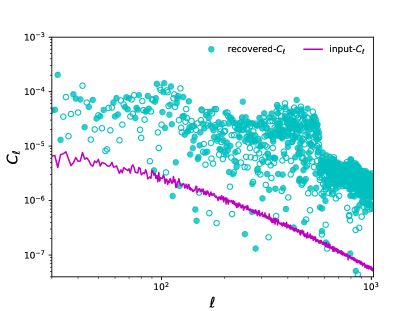
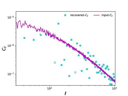
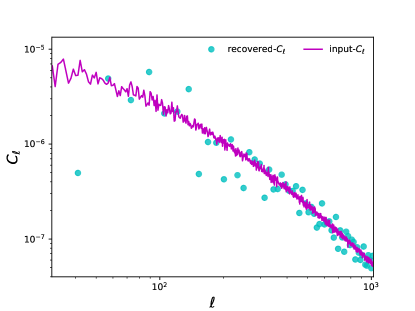
We make use of a pseudo-$C_{\ell}$ recovery algorithm by Alonso:2019 to achieve an efficient and reasonably accurate estimate of the angular power spectrum of the LoTSS DR1 catalog. The algorithm python module is publicly available as NaMaster, and the mathematical background of the estimator, its features, and software implementation are described in Alonso:2019. We test the performance of the pseudo-$C_{\ell}$ algorithm for the LoTSS DR1 mask using a test map, which resembles the LoTSS DR1 density fluctuations as follows. We obtain a reasonable recovery of $C_{\ell}$ by using an un-apodized mask shown in figure 2. To emulate the LoTSS DR1 catalog, we first generate ${a_{\ell m}}$ using LoTSS DR1 model $C_{\ell}$ ; subsequently we obtain a density contrast map from ${a_{\ell m}}$ by making use of spherical harmonics (equation 3). Next, we apply the LoTSS DR1 mask to this test map and recover $C_{\ell}$ (pseudo-$C_{\ell}$s). The results thus obtained with different configurations and settings are shown in figure 4, and above $\ell>100$ a reasonable recovery is demonstrated.

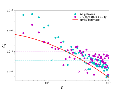
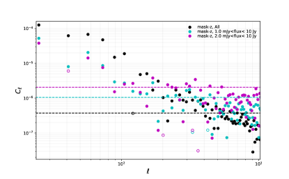
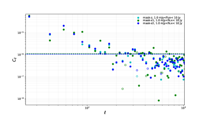
With the above demonstrated settings, we run the pseudo-$C_{\ell}$ recovery algorithm and obtain the LoTSS DR1 catalog angular power spectrum. The angular spectrum thus obtained is shown in figure 5. The recovered power spectrum for galaxies with integrated radio flux above survey completeness, i.e. $S>1$ mJy, approximately agrees with theoretical results obtained following $\Lambda$CDM and considering NVSS (Condon:1998) radio galaxy biasing and radial distribution (Adi:2015nb). Without considering survey completeness (i.e. the flux cut) the recovered power spectrum is significantly high at low $\ell$, i.e. at large scales, presumably attributing the effect of survey incompleteness. At low fluxes, when the survey is not complete, we may have large scale flux systematics and uneven source counts and thus may observe excess large scale clustering. Considering a slightly higher flux cut, i.e. $S>2$mJy, we obtain similar results as for the $S>1$ mJy flux cut $C_{\ell}$ but with slightly more fluctuations. The results are shown in figure 6. We next test the robustness of $C_{\ell}$ recovery with different masks discussed in section 2.1. With mask-z, z1 and z2 we recover almost the same $C_{\ell}$, although the fluctuations for mask-z1 are slightly higher due to low sky coverage (i.e., high cosmic variance). The results are shown in figure 7.

Depending on the flux density threshold considered, the LoTSS DR1 catalog contains a significant number of multi-component sources (Siewert:2019). The multi-component sources cause a constant offset to $C_{\ell}$. Siewert:2019 estimate the clustering parameter $n_{c}$ for LoTSS DR1, which is defined to be the ratio of the variance of counts in cells over the mean of the counts in cells. In addition they notice that the counts-in-cells statistic follows a compound Poisson distribution, assuming that the parameter $n_{c}=1+\gamma$, where $\gamma$ is the mean number of components for a source. Given this, for any source in the catalog the probability of having one or two components can be given as $\gamma\exp(-\gamma)$, or $\frac{\gamma^{2}}{2!}\exp(-\gamma)$, respectively. This implies that the ratio between the number of two-component and one-component sources equals $\gamma/2$, and thus the fraction of radio sources split into double sources i.e. $e$ as defined in Blake:2004, equals $\frac{\gamma/2}{1+\gamma/2}$. We further note from Siewert:2019 that $\gamma=0.44$ for 1 mJy flux density threshold, and estimate the multi-component offset in terms of shot-noise $\sigma_{0}$ to equal $\gamma\sigma_{0}/(1+\gamma)\approx 0.3\sigma_{0}$ for $C_{\ell}$ following Blake:2004. The estimate of course makes several assumptions as discussed above and is not guaranteed to be exact. We thus consider the multi-component offset to $C_{\ell}$s as an independent parameter in our fitting procedure. Indeed, we recover a multi-component offset close to $0.3\sigma_{0}$ as expected.

Figure 4.— Angular power spectrum recovery performance with LoTSS DR1 mask ($0.1\%$ of the sky). Empty circles show a negative value. The recovered power spectrum is significantly fluctuating as a function of multipole (top figure). Next we apodized the mask on the scale of one degree and plot $C_{\ell}$ in bands by collecting 16 multipoles per bin; we show the results for this in the middle panel. The best recovery above $\ell>100$ is obtained if we do not apodize the mask and collect 16 multipoles per bin (bottom panel).

Figure 5.— LoTSS DR1 angular power spectrum recovery. We obtain an approximate theoretical power spectrum ‘NVSS-estimate’ for LoTSS DR1 catalog following equation 8 and assuming NVSS galaxy bias and redshift distribution (Adi:2015nb). The power spectrum obtained without a flux cut is significantly high at large scales (low $\ell$). The dashed lines show the shot-noise. The LoTSS DR1 catalog is only expected to be complete above 1 mJy.

Figure 6.— LoTSS DR1 angular power spectrum recovery with different flux cuts.The empty circles show the negative value. The dashed lines show the shot-noise.

Figure 7.— LoTSS DR1 angular power spectrum recovery with mask-z,z1, and z2. These masks are described in section 2.1 and shown in figure 2. Other details same as figure 6.

6. 2-point correlation statistics

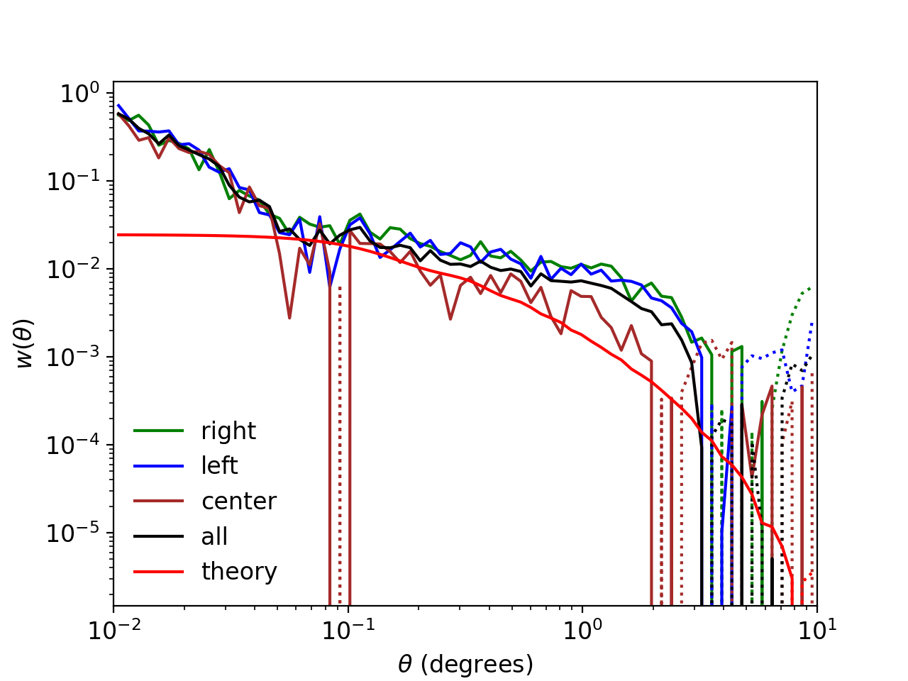
For comparison with theory and earlier results in Siewert:2019, we calculate the 2-point correlation function (2PCF) for the LoTSS DR1 catalogue. We obtain approximately the same 2PCF results with our catalog and mask, as in Siewert:2019 with 1 mJy flux cut and their mask-d. The theoretical curve at angular scales less than 0.1 degree is slightly lower than the measured values, presumably due to the multiple-component nature of some radio sources in the catalog (Blake:2004). We have followed Siewert:2019 and applied the same python package TreeCorr (Version 4.0) (Jarvis:2004) and the same parameter settings for 2PCF estimation. Following Siewert:2019 we next divide the LoTSS DR1 catalogue into three patches ‘left’, ‘center’ and ‘right’. The RA ranges for these patches are (161, 184), (184, 208), and (208, 230) degrees, respectively. The calculated angular correlation functions are shown in figure 8. We find that the center area fits the theory best. The slight mismatch between ‘left’, ‘center’ and ‘right’ patch results is an indication of large scale density fluctuation systematics present in the data. This should be considered as a motivation for refining the LoTSS DR1 pipeline (Shimwell:2019).

Figure 8.— The 2-point correlation function of LoTSS DR1 catalogues in different patches of the sky. The green curve denotes the ‘right’ patch angular correlation function, the blue for ‘left’ area and orange for ‘center’ area. The whole area angular correlation function of LoTSS DR1 is shown by the black line, while the red curve denotes the theoretical prediction following $\Lambda$CDM with NVSS bias and redshift distribution. All dotted lines represent negative values.

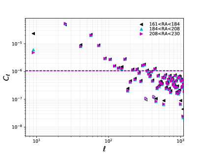
Large-scale systematics in real space correspond to low multipoles of angular power spectrum $C_{\ell}$. So to examine the effect more closely we calculate the angular power spectrum for these three right ascension patches. We show the results in figure 9 and note that $C_{\ell}$ recovery from different right ascension patches are almost the same above $\ell>10$. We recognize that $\ell=10$ corresponds to $\approx 20^{\circ}$ scale, which is approximately the right ascension patch width considered. We note that we only consider data above $\ell=100$, and for this $\ell$ range we do not see any large scale right ascension dependence.

Figure 9.— Angular power spectrum recovery of LoTSS DR1 catalogues in different patches of the sky. The recovered power spectrum from different right ascension patches is approximately the same above $\ell>10$. The dashed lines show the shot-noise.

7. Galaxy bias and $N(z)$ estimate

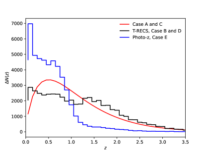
The bias $b(z)$ for each galaxy population is different and depends on the dark matter halo mass hosting the galaxy type (Mo:1996). The angular power spectrum of LoTSS DR1 in figure 4 is apparently a close match with $\Lambda$CDM estimates considering NVSS galaxies bias and redshift distribution, $N(z)$. However, in reality, the bias and $N(z)$ for LoTSS DR1 galaxies could be significantly different in comparison with values obtained for NVSS galaxies with flux above $10$ mJy (NVSS completeness) at $1.4$ GHz (Adi:2015nb; Tiwari:2016adi). The NVSS is dominantly radio loud AGNs, Fanaroff–Riley type I (FR I) and FR II (Fanaroff:1974), whereas the LoTSS DR1 above $1$ mJy contains star-forming galaxies along with radio loud AGNs, FR I and FR II type (Rivera:2017; Wilman:2008). The LoTSS DR1 population is mixed and differs from NVSS, and thus the bias $b(z)$ and $N(z)$ could be significantly different. For $N(z)$, around half of the LoTSS DR1 sources have optical/near-IR identification in Pan-STARRS/WISE and their photometric redshifts are available. The number count of these photo-identified galaxies in redshift bins ($\Delta z=0.1$) is shown in figure 10. Note that the $N(z)$ in figure 10 only represents part of the LoTSS DR1 population; the true $N(z)$ of the full LoTSS DR1 catalog could be significantly different. Nevertheless, the available photo-redshifts can be assumed to loosely represent the LoTSS DR1 galaxies’ redshift distribution. Furthermore, there are a few more reasonable $N(z)$ templates we may assume for LoTSS DR1, namely the $N(z)$ obtained for NVSS in Adi:2015nb and the $N(z)$ presented in the Tiered Radio Extragalactic Continuum Simulation (T-RECS, Bonaldi:2018).

Figure 10.— Number of radio sources per redshift bin $\Delta z=0.1$ of available z for flux density thresholds $S>1$ mJy. The redshift distributions considered for fitting $\Lambda$CDM cosmology are also shown.

Assuming a $\Lambda$CDM cosmology we seek to constrain the galaxy bias $b(z)$ and radial distribution $N(z)$ of LoTSS DR1 galaxies by fitting the measured angular power spectrum in figure 5 and the observed $N(z)$ photo-$z$ histogram in figure 10. For a given bias, $b(z)$ and $N(z)$ we calculate the theoretical (model) angular power spectrum ${C^{\rm th}_{\ell}}$. Next, we obtain the likelihood, i.e. the probability to have observed data ${C^{\rm corrected}_{\ell}}$ given the model, $\mathcal{P}({C^{\rm corrected}_{\ell}}|{b(z)},{N(z)})\propto\mathcal{L}({C^{\rm corrected}_{\ell}})\propto\exp(-\frac{1}{2}(\mathbf{{C^{\rm corrected}_{\ell}}}-\mathbf{{C^{\rm th}_{\ell}}})^{T}\mathbf{\Sigma^{-1}}(\mathbf{{C^{\rm corrected}_{\ell}}}-\mathbf{{C^{\rm th}_{\ell}}}))$. Here $\mathbf{\Sigma}$ is the covariance matrix computed using mocks discussed in Section 3. We make use of Bayes’ probability theorem, and write the model probability given the data, $\mathcal{P}({b(z)},{N(z)}|{C^{\rm corrected}_{\ell}})=\mathcal{P}({C^{\rm corrected}_{\ell}}|{b(z)},{N(z)})\times\mathcal{P}({b(z)})$. Here $\mathcal{P}({b(z)})$ is the prior probability of bias ${b(z)}$.

Figure 11.— The pipeline recovers input bias parameters within one $\sigma$, dashed lines are input values. The figure in particular demonstrates the quadratic bias $b(z)=b_{0}+b_{1}z+b_{2}z^{2}$ recovery. For our fitting range, i.e. $\ell=200-1000$, we do not cover enough power spectrum shape to constrain $b_{1}$ and $b_{2}$ and the posterior probability for these are almost the same as the prior information we assume.

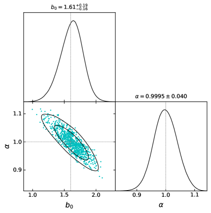
We assume different $N(z)$ templates and run an MCMC sampler to maximize model parameter probability, $\mathcal{P}({b(z)},{N(z)}|{C^{\rm corrected}_{\ell}})$, i.e. obtain the best fit to $\Lambda$CDM cosmology and deduce effective bias $b(z)$, given the $N(z)$ values. We fit one more model parameter, $\alpha$, to account for the multi-component offset to ${C^{\rm corrected}_{\ell}}$ as discussed in sections 4 and 5. We conveniently use Cobaya (Torrado:2020xyz) to perform Bayesian analysis and CosmoMC (Lewis:2002ah; Lewis:2013hha) for MCMC sampling. With mock catalogs, we verify the above MCMC pipeline and recover the input bias within one sigma uncertainty for the $\ell=200$ to $1000$ range. The pipeline performance is demonstrated in figure 11. Above $\ell=1000$ the recovery from mocks is noisy and therefore we restrict our fits to $\ell\leq 1000$ for all cases discussed below. We would like to emphasize that the measured $C_{\ell}$ are projected quantities, and it is hard to extract tomographic information from them. The recovered bias is strongly dependent on the $N(z)$ assumption; the best we can do for now is to assume a variety of $N(z)$ models for the LoTSS catalog. We hope to have better $N(z)$ observations in future and thus better constraints on $b(z)$.

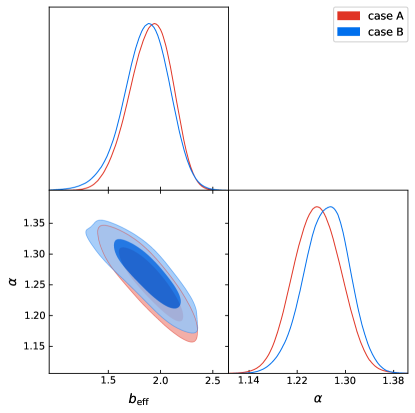
Case A: Assume $N(z)\sim z^{0.74}\exp\left[-\left(\frac{z}{0.71}\right)^{1.1}\right]$ as given in Adi:2015nb; we fit an effective redshift independent bias and shot-noise factor $\alpha$. We find that a bias $b_{\rm eff}=1.90\pm{0.20}$ fits best with the data. The recovered best fit angular power spectrum is shown in figure LABEL:fig:best_Cl. The recovered shot-noise factor is $1.25\pm 0.04$ which is consistent with $1.30$ as expected in section 5.

Case B: We employ the T-RECS (Bonaldi:2018) simulation, and produce an $N(z)$ histogram considering the SFG+AGN population above 1 mJy flux at 150 MHz. The histogram is shown in figure 10. We assume the T-RECS histogram in figure 10 represents the LoTSS population and run the MCMC sampler to find the best redshift independent bias value. We obtain $b_{\rm eff}=1.86\pm{0.22}$ as best fit to the data. The best fit angular power spectrum and bias with one sigma uncertainty band is shown in figures LABEL:fig:best_Cl and LABEL:fig:best_bz, respectively.

Figure 12.— Case A and B: Posterior distributions of bias and shot-noise factor $\alpha$. $(\alpha-1)\times\sigma_{0}$ is the multi-component offset.

Case C: $N(z)$ same as in case A; we fit a quadratic bias $b(z)=b_{0}+b_{1}z+b_{2}z^{2}$. This is to test how well NVSS quadratic bias obtained in Adi:2015nb fits to LoTSS DR1. We have noticed with mocks that the data is not sensitive to $b_{1}$ and $b_{2}$, we recover the same posterior probability for these as the prior information we assume. We fix these to NVSS observed values, i.e. $b_{1}=0.85$, $b_{2}=0.33$ and run the MCMC sampler over $b_{0}$ and noise+multi-component factor $\alpha$. The best-fit bias, $b(z)$, and angular power spectrum thus recovered are shown in figures LABEL:fig:best_bz and LABEL:fig:best_Cl, respectively. The MCMC sample and posterior distributions are shown in figure 13. We do see a better fit with quadratic bias; the fit parameters AIC and BIC are slightly improved. All parameters, their prior information and fit parameters are given in table 7.

Figure 13.— Case C and D: One and two-dimensional posterior distributions of quadratic bias free parameters $b_{0}$ and shot-noise factor $\alpha$. As the data is not sensitive to $b_{1}$ and $b_{2}$, we fix these to NVSS observed values. Other details same as in figure 12.

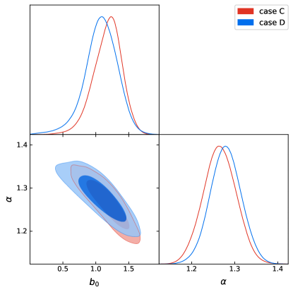
Case D: We choose $N(z)$ to be the same as in case B, and fit a quadratic bias $b(z)=b_{0}+b_{1}z+b_{2}z^{2}$. Other details are the same as in case C. The recovered best bias, $b(z)$, and angular power spectrum are shown in figures LABEL:fig:best_bz and LABEL:fig:best_Cl, respectively. The MCMC sample and posterior distributions are shown in figure 13.

Case E: Finally, we use observed photo-z redshifts which are available for onlyy about half of the radio sources. This $N(z)$ only represents part of the LoTSS DR1 population, but we include this case to check the sensitivity of the data to $N(z)$. We assume a redshift independent bias, i.e. $b(z)=b_{\rm eff}$ and a shot-noise factor $\alpha$, and then fit with the recovered LoTSS DR1 angular power spectrum. We obtain a best fit bias $b_{\rm eff}=1.05\pm{0.10}$. The recovered best power spectrum is shown in figure LABEL:fig:best_Cl.

Figure 14.— Case E: Posterior distributions of bias and shot-noise factor $\alpha$. Other details same as in figure 12.

Table 1MCMC sampler results. The prior and maximum likelihood value of the model free parameters and uncertainties. The flat prior range is shown in square brackets.The reduced $\chi^{2}$, i.e. $\chi^{2}$ per degree of freedom, AIC and BIC are also listed for model fit comparison.

		Case A	Case B	Case C	Case D	Case E
$b_{{}_{0}}$	prior			$[0.0,5.0]$	$[0.0,5.0]$
	fit value	–	–	$1.18\pm{0.22}$	$1.08\pm{0.25}$	–
$b_{{}_{1}}$	fix			$0.85$	$0.85$
$b_{{}_{2}}$	fix			$0.33$	$0.33$
$b_{\rm eff}$	prior	[0.5, 5.0]	[0.1, 5.0]			[0.1, 5.0]
	fit value	$1.90\pm{0.20}$	$1.86\pm{0.22}$	–	–	$1.05\pm{0.10}$
$\alpha$	prior	[0.01, 3.0]	[0.01, 3.0]	[0.01, 3.0]	[0.01, 3.0]	[0.01 3.0]
	fit value	$1.25\pm{0.04}$	$1.27\pm{0.04}$	$1.26\pm{0.04}$	$1.28\pm{0.04}$	$1.22\pm{0.04}$
$\bm{\chi^{2}}$/dof		1.18	1.36	1.18	1.36	1.39
AIC		60.65	69.28	60.49	69.06	70.66
BIC		64.47	73.11	64.32	72.88	74.48