Extracting the 21 cm EoR signal using MWA drift scan data

Abstract

The detection of redshifted hyperfine line of neutral hydrogen (HI) is the most promising probe of the Epoch of Reionization (EoR). We report an analysis of 55 hours of Murchison Widefield Array (MWA) Phase II drift scan EoR data. The data correspond to a central frequency $\nu_{0}=154.24\,\rm MHz$ ($z\simeq 8.2$ for the redshifted HI hyperfine line) and bandwidth $B=10.24\,\rm MHz$. As one expects greater system stability in a drift scan, we test the system stability by comparing the extracted power spectra from data with noise simulations and show that the power spectra for the cleanest data behave as thermal noise. We compute the HI power spectrum as a function of time in one and two dimensions. The best upper limit on the one-dimensional power spectrum are: $\Delta^{2}(k)\simeq(1000~{}\rm mK)^{2}$ at $k\simeq 0.2$$h~{}{\rm Mpc}^{-1}$and at $k\simeq 1$$h~{}{\rm Mpc}^{-1}$. The cleanest modes, which might be the most suited for obtaining the optimal signal-to-noise, correspond to $k\gtrsim 1$$h~{}{\rm Mpc}^{-1}$. We also study the time-dependence of the foreground-dominated modes in a drift scan and compare with the expected behaviour.

1 Introduction

The probe of the end of cosmic dark age remains an outstanding issue in modern cosmology. From theoretical considerations, we expect the first luminous objects to appear at a redshift $z\simeq 30$. The ultraviolet and other radiation from these first sources ionized and heated the neutral hydrogen (HI) in their neighbourhood. As the universe evolved, these ionized regions grew and merged, resulting in a fully ionized universe by $z\simeq 6$, as suggested by the measurements of Gunn-Peterson troughs of quasars (Fan et al. 2006). Recent Planck results on cosmic microwave background (CMB) temperature and polarization anisotropies fix the reionization epoch at $z\simeq 7.8$ (Planck Collaboration et al. 2020). The cosmic time between the formation of the first light sources ($z\simeq 30$, the era of cosmic dawn) and the universe becoming fully ionized ($z\simeq 6$) is generally referred to as the Epoch of Reionization (EoR).

Many important astrophysical processes during this era, e.g. the formation of first light sources and the evolution of ionized regions around them, can be best probed using the hyperfine transition of the neutral hydrogen atom. Due to the expansion of the universe, this line of rest frame frequency $\nu\simeq 1.4\,\rm GHz$, redshifts to frequencies 70–200 MHz ($z\simeq 6\hbox{--}20$), which can be detected using meter-wave radio telescopes.

Several existing and upcoming radio telescopes aim to detect both the sky-averaged and the fluctuating component of redshifted HI signal, e.g. radio interferometers—Murchison Widefield Array (MWA Tingay et al. 2013, Bowman et al. 2013), Low Frequency Array (LOFAR van Haarlem et al. 2013), Donald C. Backer Precision Array for Probing the Epoch of Reionization (PAPER Parsons et al. 2014), Hydrogen Epoch of Reionization Array (HERA DeBoer et al. 2017), and the Giant Metrewave Radio Telescope (GMRT, Paciga et al. 2013). In addition there are multiple ongoing experiments to detect the global HI signal from this era—e.g. EDGES and SARAS (Bowman et al. 2018, Singh et al. 2018).

We focus on the fluctuating component of the HI signal in this paper. There are considerable difficulties in the detection of this signal. Theoretical studies suggest that the strength of this signal is of the order of 10 mK at $150~{}\rm MHz$ while the foregrounds are brighter than 100 K (for detailed review see Furlanetto et al. 2006, Morales & Wyithe 2010, Pritchard & Loeb 2012). These foreground contaminants include the diffuse galactic synchrotron emission and the extragalactic radio sources. Current experiments can reduce the thermal noise of the system to suitable levels in many hundreds of hours of integration. The foregrounds can potentially be mitigated by using the fact that the HI signal and its correlations emanate from the three-dimensional structures of mega-parsec scales at high redshifts. On the the other hand, the foreground contamination is dominated by spectrally smooth sources. This means that even if foregrounds can mimic the HI signal on the plane of the sky, the third axis, corresponding to the frequency, can be used to distinguish between the two. All ongoing experiments exploit this spectral distinction to isolate the HI signal from the foreground contamination (e.g. Parsons & Backer 2009, Parsons et al. 2012).

Many image and visibility-based pipelines have been developed to analyze the interferometric data. These have yielded upper limits on the HI signal for the EoR (Paciga et al. 2013; Dillon et al. 2015; Paul et al. 2016b; Beardsley et al. 2016; Choudhuri et al. 2016; Trott et al. 2016; Patil et al. 2017; Kolopanis et al. 2019; Li et al. 2019; Barry et al. 2019; Mertens et al. 2020; Trott et al. 2020). The current best upper limits on the HI power spectrum lie in the range: $\simeq(50~{}\rm mK)^{2}\hbox{--}(75~{}\rm mK)^{2}$ for $k\simeq 0.05\hbox{--}0.2$$h~{}{\rm Mpc}^{-1}$in the redshift range $6.5\hbox{--}10$. More recently, Bowman et al. (2018) reported the detection of an absorption trough of strength $\simeq 500~{}{\rm mK}$ in the global HI signal in the redshift range $15<z<19$.

Some of the key requirements for the detection of the weak HI signal are extreme stability of the system, precise calibration, and reliable isolation of foregrounds. Drift scans constitute a powerful method to achieve instrumental stability during an observational run. During such a scan the primary beam and other instrumental parameters remain unchanged while the sky intensity pattern changes. Two interferometers, PAPER (PAPER is no longer operational) and HERA, work mainly in this mode while other telescopes (e.g. MWA) can also acquire data in the drift scan mode. Different variants of drift scans have been proposed in the literature: $m$-mode analysis (Shaw et al. 2014, 2015, applied to OVRO-LWA data in Eastwood et al. 2018), cross-correlation of the HI signal in time (Paul et al. 2014), drift and shift method (Trott 2014) and fringe-rate method (Parsons et al. 2016, applied to PAPER data).

In this paper, we present the results of the analysis of 55 hours of drift scan MWA Phase II data. The data was taken over 10 nights with repeated scans of duration 5.5 hours over the same region of the sky. The feasibility of drift scan using MWA has been studied theoretically (Trott 2014; Paul et al. 2014; Patwa & Sethi 2019). In this paper, we use the formalism developed by Patwa & Sethi (2019). We work in delay space, which isolates foregrounds from the EoR window and is therefore the natural domain of power spectrum measurement (e.g. Datta et al. 2010, Parsons et al. 2012).

We develop a pipeline for measuring the 21 cm HI power spectrum for drift scans in the delay space. In section 2, we describe the MWA phase II EoR data and its pre-processing, e.g. flagging, time-averaging, and processing using Common Astronomy Software Application (CASA; McMullin et al. 2007). In section 3, we briefly review different methods of extracting the HI signal from drift scan data and provide justification for the method adopted in this paper. In section 4, we discuss the transformation of the gridded data to the delay space and outline techniques needed for the estimation of the HI power spectrum from the data. In section 5, the main results are presented. In this section, we first characterize the noise properties of the data and study the stability of the system over the duration of the scan by comparing the data power spectrum with noise simulations. In section 5.2, we apply our methods to extract the HI power spectra in different representations of the HI signal in Fourier space. Finally, the behaviour of the foreground-dominated modes of the data is discussed in a drift scan. We summarize our results and conclude with possible future directions of our work in Section 6.

Throughout this paper we use the spatially-flat $\Lambda$CDM model for our work with values $h=0.67$, $\Omega_{\Lambda}=0.6911$, $\Omega_{m}=0.3089$, $\Omega_{k}=0.0$ (Planck Collaboration et al. (2020)).

2 data

Murchison Widefield Array (MWA) is a radio interferometer located in Western Australia at a latitude of $-26.7^{\circ}$ and longitude of $116.7^{\circ}$. It has 128 tiles (a tile would be referred to as an antenna in the paper) and each tile consists of 16 crossed dipoles placed on a square mesh of length $\sim 4~{}{\rm m}$ in a 4x4 arrangement. It operates in the frequency range of 80–300 MHz with an observational bandwidth of 30 MHz and a frequency resolution (channel width) of 40 kHz. The visibility data is recorded at an interval of 2 minutes with the temporal resolution of 0.5 s. In each 2-minute snapshot, the duration of observation is 112 s. In the Phase II design of MWA, 64 antennas are placed in a compact Hex configuration to increase the number of short and redundant baselines primarily for EoR studies. The instantaneous baseline distribution of MWA Phase II for a zenith scan is shown in Figure 1 (e.g. See Tingay et al. 2013; Wayth et al. 2018 for a detailed description of the MWA design).

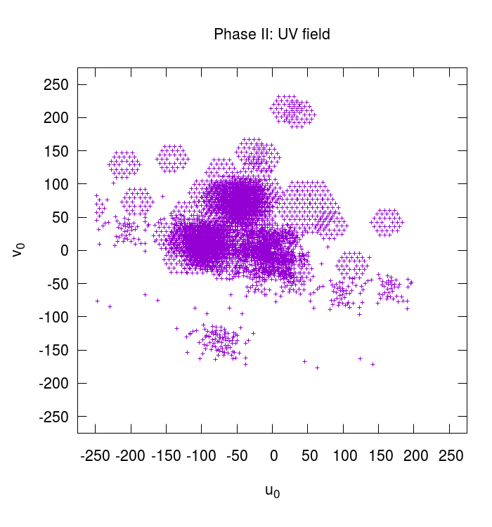
Figure 1: MWA Phase II baseline distribution for a zenith drift scan (in the units of central wavelengths $\lambda_{0}=1.95~{}\rm m$)

2.1 Metadata

In Figure 2 we display the region of the sky covered by the drift scans with the MWA. The drift scan data we use in this paper was acquired in 2016 (Paul et al., 2016a) and at the time of the analysis was publicly available in the MWA Data Archive with project ID G0031. Each scan lasted 5 hrs 24 minutes and was repeated across the same region of the sky for 10 consecutive nights from 2016-Oct-03 to 2016-Oct-12. The scanned region covers a portion of the sky from the position of the EoR0 ($0{\rm h},-27^{\circ}$) to the EoR1 ($4{\rm h},-27^{\circ}$) fields of the MWA. Each night the scan was carried out between 14:39 UTC and 19:28 UTC. On the sixth night, nearly two hours of data was missing during the initial period and the scan lasted only 3 hrs 10 minutes.

The reported sky temperatures in the regions covered by the scan vary in the range $210$–$267$ K. The scan also passes over Fornax A which is an extended radio source with a core and two radio lobes. Its angular extent spans the region, RA $3{\rm h}25{\rm m}$ to $3{\rm h}20{\rm m}30{\rm s}$ and Dec $-37^{\circ}30^{\prime}$ to $-36^{\circ}54^{\prime}$. The total flux density of this source at 154 MHz is 750 Jy (McKinley et al. 2015).

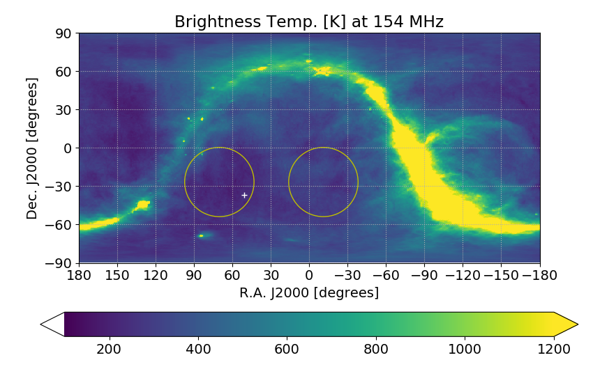
Figure 2: This figure displays the Haslam map scaled to 154 MHz assuming the brightness temperature spectral index $\alpha=-2.52$ (Rogers & Bowman 2008). The big circles denote the main lobe of the MWA primary beam at $\nu=154\,\rm MHz$. The scan starts roughly at the location of the circle on the right and lasts until the field of view corresponds to the circle on the left. The white ‘+’ sign shows the position of Fornax A.

2.2 Flagging, calibration, and averaging

COTTER is a pre-processing pipeline which flags RFI, non-working antennas and frequency channels (Offringa et al. 2015). It also does cable correction, can average data and produce CASA readable Measurement Sets (called MS tables/files). We apply COTTER on all 2 minute snapshots individually and average them to 10 s time resolution, with the frequency resolution kept intact (40 kHz). The MWA publicly-available archive provides COTTER to enable the reduction in the data volume. COTTER was applied on-site before the data was downloaded. In each 2-minute data file, as noted above, the observation span is 112s. Thus, after time-averaging there are 11 data chunks in each 2-minute data file. We then apply the bandpass and the flux density calibration with the strong and unresolved calibrator source Pictor A.

The calibration solution tables also help in identifying and flagging unresponsive or irregularly behaving antennas and baselines. Next we flag the channels situated at either ends of the coarse bands of MWA bandpass.

These processes yield calibrated time-ordered visibility data-sets of 10 nights. We then performed averaging over data from different nights. Since the drift scans cover the same region of the sky, we carry out LST stacking (this is the usual procedure to add data for all transit radio telescopes e.g. Bandura et al. (2014)) which constitutes aligning and averaging data snapshots with the same tracking centers, baseline bins (see below for more details), and frequency channels observed on different nights. After LST stacking, we obtain the equivalent of one night of drift scan data over the same region of the sky. These data are suitable for the EoR power spectrum analysis.

3 Data analysis methodology

Many operational radio interferometers rely on drift scans to extract the power spectrum of the intensity of redshifted HI line from the EoR and low redshift data (Bandura et al. 2014; Kolopanis et al. 2019; Parsons et al. 2016; DeBoer et al. 2017). CHIME adopts m-mode decomposition of the time-ordered visibility data, which relies upon Fourier transforming the data stream. PAPER and HERA use weighted averages of the visibility data. In Patwa & Sethi (2019) (hereafter PS19), we proposed many different approaches to analysing the drift scan data and showed similarities and differences between existing methods. In this paper, we adopt a method based on cross-correlating the time-ordered visibilities (for details see PS19).

The main aim of all the analysis pipelines is to construct an unbiased and optimal estimator to extract the HI power spectrum from the visibility data in frequency or delay space. Unlike the tracking data, the intensity pattern in a drift scan changes with respect to the beam, and the analysis of these time-dependent visibilities arising from a changing intensity pattern presents new challenges.

All the methods of extracting the HI power spectrum directly from the visibility data are based on the correlation properties of the measured visibility $V_{\nu}(\textbf{u}_{\nu},w_{\nu},t)$ in different domains. These properties have been well studied for the tracking data for frequency and baseline domains and can readily be extended to the drift scan data (e.g. PS19). Here our focus is the correlation of measured visibilities in the time domain. PS19 derived the de-correlation profile for the primary beams of many operational and future interferometers. Even though this profile is a complicated function of the baseline length, the de-correlation time varies between a few minutes to 30 minutes for most interferometers. As the visibility data generally has higher time resolution as compared to the de-correlation time, e.g. we use MWA data with 10 second resolution in this paper, multiple methods can be used to analyse the data. In the analysis of PAPER data, a time filter is used to average over visibilities which contribute coherently to the HI signal (e.g. Kolopanis et al. 2019 uses 43-second time filters). As already noted above, CHIME data analysis is based on Fourier transforming the time-ordered visibility data (for details see PS19).

In our work, we adopt the method based on cross-correlation of visibilities in time (PS19). This method is applicable to both frequency and delay space data. In this work, we transform visibility to delay space to isolate foregrounds. The HI power spectrum is extracted using the estimator (Eq. (45) of PS19) for $t\neq t^{\prime}$ to avoid noise bias:

$${\cal C}_{\tau} (\textbf{u}_{0},w_{0})$$

$$=\frac{\sum_{t^{\prime},t}\exp(-i2\pi u_{0}\cos{\phi}\Delta H)V_{\tau}(\textbf{u}_{0},w_{0},t)V_{\tau}(\textbf{u}_{0},w_{0},t^{\prime})^{*}g(t^{\prime}-t)}{\sum_{t^{\prime},t}g^{2}(t^{\prime}-t)}$$ (1)

Here $g(t^{\prime}-t)$ is the function that captures the de-correlation of visibilities as a function of the time difference $t^{\prime}-t$ (Figure 1 of PS19). $g(t^{\prime}-t)$ is nearly unity for $t^{\prime}-t<20$ minutes for the shortest baselines we consider in this paper, $\sqrt{u^{2}+v^{2}}\simeq 20$ and the de-correlation time scale falls to around 5 minutes for the longest baselines, $\sqrt{u^{2}+v^{2}}\simeq 300$. $\Delta H$ is the difference of the hour angle between times $t$ and $t^{\prime}$. $\tau$ is the delay space parameter and $\textbf{u}_{0}\equiv(u_{0},v_{0})$ and $w_{0}$ are the baselines and the $w$-term at the center of the bandpass. As shown in PS19, this estimator is both unbiased and optimal for the extraction of the HI signal. The measured quantity (Eq. (1)) is converted to the variables of the HI signal using relations given in Appendix A.

4 Data Analysis

The visibilities in delay space can be derived from the visibilities in the frequency space by performing a discrete Fourier transform:

$$V_{\tau}(\textbf{u}_{0},w_{0},t)=\Delta\sum_{\nu_{0}-\frac{B}{2}}^{\nu_{0}+\frac{B}{2}}V_{\nu}(\textbf{u}_{\nu},w_{\nu},t)B_{\nu}e^{2\pi i\tau\nu}.$$ (2)

For our analysis, the central frequency, $\nu_{0}=154.24\,\rm MHz$ and $B=10.24\,\rm MHz$, which yields 256 channels of channel width $\Delta=40\,\rm KHz$. $B_{\nu}$ corresponds to Blackman-Nuttall window (Nuttall 1981), which helps reduce power leakage between delay bins. Our analysis is entirely based on analysing the visibilities and their correlations and at no stage do we transform to the image domain. We also do not subtract foreground sources based on any model of foregrounds but rely on the separation of foregrounds from the EoR signal in delay space.

4.1 Gridding of UV field and power spectrum estimation

In Figure 1, we display the baseline distribution of MWA Phase II for our observational setting (zenith scan). In a drift scan, the UV distribution and the $w$-term are left unchanged. For zenith scans, the $w$-term is generally small, $|w_{0}|\leq 3\lambda_{0}$ for MWA, and its impact on the interpretation of data can be neglected (for details e.g. see PS19). We select a square UV field with $u_{0}$ and $v_{0}$ in the range: $-250\lambda_{0}$ to $+250\lambda_{0}$. This allows us to include all the UV regions in which the density of baselines is large for MWA Phase II (Figure 1).

For analysing the data, we grid the UV field, with the size of a pixel determined by the expected behaviour of the HI signal. It can readily be shown that, for MWA, the HI signal de-correlates for baselines that differ by more than a few wavelengths (e.g. Morales & Hewitt 2004, Paul et al. 2016b and references therein). We choose a square pixel of $0.5\lambda_{0}$ so that the equal-time visibilities are coherent inside a grid; the baselines are assigned the same value inside a pixel. We also assume inter-pixel visibilities to be uncorrelated. Each UV pixel also has non-zero width in delay space ($\simeq 1/B$) owing to finite bandwidth. For every UV grid, the HI signal is coherent within this width (e.g. PS19, Paul et al. (2014); Parsons et al. (2016) and references therein). We refer to this three-dimensional grid, labelled by ${\bf u}_{0},\tau$, as ‘voxel’ in the rest of the paper.

We populate the gridded UV field (for a given $\tau$) with visibility data (each data point corresponds to an integration time $t_{\rm int}=10$ s). For the combined data of 10 nights, the number of voxels and the maximum occupancy of a voxel for a fixed $\tau$ and time are 5427 and 55, respectively (Figure 1).

The correlation function (Eq. (1)) (and the power spectrum using Eq. (6)) can be computed from the gridded data for a given voxel. This procedure can be extended to further compute mean power spectra, by carrying out a weighted average (the weight can be theoretically computed from the occupancy of a given voxel): (a) over all the voxels for a fixed $\tau$, (b) over a set of voxels for a given $k_{\parallel}$ and $|{\bf k_{\perp}}|$, or (c) a set of voxels for a fixed $|{\bf k}|=\sqrt{{\bf k_{\perp}}^{2}+k_{\parallel}^{2}}$. All these quantities can be estimated as a function of integration (or drift) time. These averages are in units of $(\rm JyHz)^{2}$; they are converted to $({\rm mK})^{2}(h^{-1}\rm Mpc)^{3}$using Eq. (6). The estimated power spectrum is a complex number. Throughout this paper, while displaying the power spectrum, we plot the absolute value of this complex number.

5 Results

Given that the expected HI signal can only be detected after hundreds of hours of integration, it is imperative that the noise of the instrument is characterized precisely—this allows us to gauge the stability of the system, e.g. primary beam and bandpass, and the extent of foreground contamination. In this paper, we analyze 55 hours of drift scan data in delay space and expect the data for a fraction of delay space parameters to be dominated by noise. We attempt to verify this hypothesis in the next sub-section.

5.1 Noise characteristics

There are multiple ways to compare the data with noise simulations. The most straightforward method would be to compare the HI power spectrum extracted from data against simulated visibilities. We do not adopt this method for the following reason. If there are $N$ visibility measurements in a pixel, there are a total of $N(N-1)/2$ cross-correlations. However, the HI power spectrum is based on only a fraction of these cross-correlations as the HI signal de-correlates for $t^{\prime}-t$ exceeding 30 minutes for even the shortest baselines we study here. For noise characterization, we give equal weight to all cross-correlations, which is equivalent to $g(t^{\prime}-t)=1$ in Eq. (1). This also allows us to use the pipeline developed for the extraction of HI signal with minor modifications on the data and simulated visibilities.

For comparison with data, we simulate visibility data using Gaussian random noise. In this case, each visibility cross-correlation has zero mean (because all visibilities are uncorrelated), and an RMS $\sigma$ given by (Christiansen & Hoegbom 1969):

$$\sigma=\frac{1}{\eta_{s}}\frac{2k_{B}T_{\rm sys}}{A_{\rm eff}\sqrt{\Delta\nu t_{\rm int}}}.$$ (3)

For the simulation, the following MWA system parameters are used: $A_{\rm eff}=21.4{~{}\rm m}^{2}$, $\Delta\nu=40$ kHz, $t_{\rm int}=10$ s. In addition, we assume $\eta_{s}=1$, and $T_{\rm sys}=400$ K. This yields an RMS for a single cross-correlation, $\sigma=81.8$ Jy. We note that the comparison of noise simulations with data allows us to determine $T_{\rm sys}/\eta_{s}$. We transform these simulated visibilities to delay domain for the baseline distribution of MWA Phase II.

In a given voxel, the number of cross-correlations increase as the square of the drift time, $t^{2}$. If all the cross-correlation are assigned equal weight, the RMS of the power spectrum computed from all cross-correlations within a voxel is expected to scale as $1/t$. This motivates us to define the following function for comparing the simulated noise with the data:

$$f(t)=a\left(\frac{120\,{\rm sec}}{t}\right)$$ (4)

where $a$ and $t$ are in units of $({\rm mK})^{2}(h^{-1}\rm Mpc)^{3}$and seconds, respectively.

$a~{}[10^{10}\text{$({\rm mK})^{2}(h^{-1}\rm Mpc)^{3}$}]$	XX	YY
Night 1	5.9	7.4
Night 2	5.3	6.9
Night 3	7.3	9
Night 4	5.6	7.4
Night 5	6.4	8.3
Night 6	4.2	5.4
Night 7	6.3	8
Night 8	5.8	7.3
Night 9	6.2	8.1
Night 10	5.8	7.5
Mean	5.9	7.5

Table 1: The table displays the normalization defined in Eq. (4) for the 10-night data for both XX and YY polarizations.

In Table (1) we display the results of 10 nights of data. The coefficient $a$ in Eq. (4) is computed using the first half an hour data on every night for the delay parameters with the lowest RMS. Night 6 data gives a smaller value because there is no data on that night for the first two hours and the data flow starts from a slightly cooler region of the sky. From simulated visibilities we obtain $a\simeq 11.7\times 10^{10}$$({\rm mK})^{2}(h^{-1}\rm Mpc)^{3}$, which is higher than the data for $T_{\rm sys}/\eta_{s}=400\,\rm K$. A comparison with data allows us to infer $250\,{\rm K}<T_{\rm sys}/\eta_{s}<330\,\rm{\rm K}$. For $\eta_{s}\simeq 1$, the estimated system temperature is in good agreement with the reported range of system temperatures in the scanned region of the sky.

When the data from all the nights is combined, we obtain $a=8.4\times 10^{9}$$({\rm mK})^{2}(h^{-1}\rm Mpc)^{3}$for XX and $a=10.4\times 10^{9}$$({\rm mK})^{2}(h^{-1}\rm Mpc)^{3}$for YY. A comparison with the values in Table (1) shows that the improvement for the combined 10 nights of data is a factor of 7 (XX polarization) and 7.2 (YY polarization) while the decrement under the ideal conditions would be closer to a factor of 10.

Figure 3 shows both the simulated noise and the data as a function of drift time. The figures display the mean power spectra and the RMS of mean power spectra for Gaussian Noise (GN) simulations and the combined data sets of 10 nights. Different lines (129 lines) in the figures correspond to the values of the delay parameter $\tau$ (including $\tau=0$). The data is also compared to the expected analytic function (Eq. (4)).

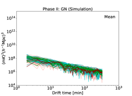
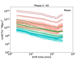
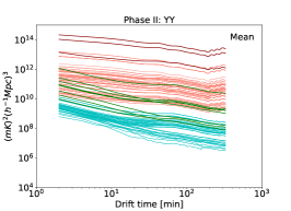
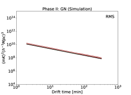
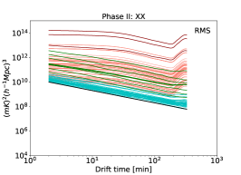
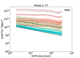
Figure 3: The mean power spectra along with the RMS of power spectra for one voxel are displayed as a function of drift time (in minutes). The first column shows the outcome of Gaussian noise (GN) simulations for the baseline distribution of MWA Phase II. The second and third columns give results for XX and YY polarization, respectively. The first row shows the mean power spectrum while the second row displays the RMS of the power spectra. The horizontal axis in all the plots corresponds to the drift time. There are 129 curves in every panel, each corresponding to a different value of the delay space parameter $\tau$ (including $\tau=0$). The dark and the light red coloured curves represent the wedge and horizontal bands (including two modes on either side of the band), respectively. The rest of the modes in the EoR window are divided into two colours: intermediate values of $\tau$ in green and the clean modes corresponding to $\tau\geq 22$ (in units of $B^{-1}$) in light blue. Thick black line in the RMS plots correspond to the function given in Eq. (4).

Figure 3 has been demarcated into several regions to separate the delay parameters suitable for the EoR detection from the foreground dominated modes. This figure should be viewed in conjunction with the more usual wedge plot (Figure 7). The dark red lines correspond to the delay parameters that are most contaminated by foregrounds ($\tau\la 10/B$). The light red lines capture the impact of missing channels in MWA. We find the delay parameters $\tau<22/B$ to be partially contaminated by foregrounds and this region is delineated by green lines. The cleanest regions correspond to light blue lines which correspond to delay parameters which are separated from horizontal bands (caused by missing channels) by more than $1/B$ and $\tau>22/B$. These regions will be referred to as ‘clean modes’ in the rest of the paper. These modes constitute 25–30% of the delay parameters. The figure shows that the signal (the mean and the RMS) could vary by over an order of magnitude even within the clean modes, which partly captures the variation of the mean even for noise dominated modes (the upper left panel of the figure). However, the noise RMS clusters around a line (the lower left panel of the figure) which suggests that some of the clean modes could be affected by residual foreground contamination and other systematic errors. However, Figure 3 also shows that the RMS in the noise simulation and the RMS in the clean modes from data (both XX and YY polarizations) decrease as $1/t$ (Eq. (4)). This provides clear evidence that the clean modes are noise-dominated. For the clean modes, there is reduction of noise by nearly two orders of magnitude over 4 hrs, as anticipated by the analytic fit (Eq. (4)).

The data power spectra begin to deviate from noise simulations after nearly four hours of drift scan, which is related to a corresponding increase in the mean power and the RMS in foreground-dominated modes towards the end of the scan. This increase can be understood from Figure 2. It is caused when the bright radio source Fornax A enters the main lobe of the primary beam and sidelobe pick up by the emission from the galactic plane.

To test the hypothesis that this enhancement in the power towards the end of the scan is caused by extended sources such as Fornax and the galactic plane, we re-analyse data by excluding smaller baselines ($<100\lambda_{0}$). We find that this procedure removes the bump. This shows that extended sources, even with complex structures, can be removed if small baselines are ignored in power spectra computation. However, since the HI signal is expected to be stronger on smaller baselines, this procedure is only used for testing and not for the final analysis of data.

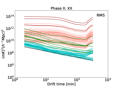
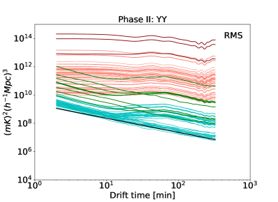
Figure 4: The panels display the RMS of the power spectrum by re-defining the power spectrum as the weighted average over randomly-chosen 100 voxels which yields 54 data sets. The RMS is computed from these sets. The mean power spectrum is left unchanged by this procedure. The colour scheme is the same as in Figure 3. The expected decrement in RMS for thermal noise is approximately a factor of 10, which is seen in the clean modes; the wedge and the horizontal bands which are foreground-dominated do not show this behaviour.

In the foregoing, we performed all the visibility cross-correlations (with the same weight) inside a voxel and computed the average and the RMS of this quantity over all the voxels (5427 voxels for a given delay parameter $\tau$). This yields the mean power spectrum and the RMS of the power spectrum of a voxel as a function of drift time. For further noise testing, all the voxels are divided into sets of randomly-selected 100 voxels. This yields 54 sets for a given $\tau$. The power spectrum is computed for each set and then the mean and RMS is computed by performing weighted averaging over all the sets. For thermal noise, we expect the RMS to reduce by a factor of $\sqrt{100}$. Figure 4 shows the RMS after this procedure. The ratio of the new to the old lower envelope is nearly a factor of 10, in consonance with the expected decrement. We do not show the mean of the signal in Figures 4 because the computation of the mean involves a linear process so it does not matter whether it is computed using all the grids or first computed over 100 grids and then averaged over the remaining grids.

The expected decrement in the RMS after the second level of averaging (Figure 4) provides further evidence that a fraction of the data is uncorrupted by either systematic errors or foregrounds and therefore is useful for the detection of the HI signal.

Another interesting feature of the figures is gradual decrease in the power for the modes that are contaminated by foregrounds. This will be discussed in detail in the next section.

5.2 HI power spectrum

As explained above, the HI power spectrum can be estimated from the gridded visibility data using Eq. (1) and the relations given in the Appendix. The main input into this estimation is the function $g(t^{\prime}-t)$ which determines the time dependence of the coherence of the HI signal, as a function of baseline, for the primary beam of MWA (for further details see PS19). In this section we present results for the HI power spectrum and its RMS for the combined 10-night data.

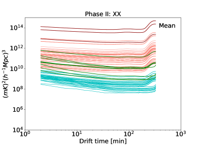
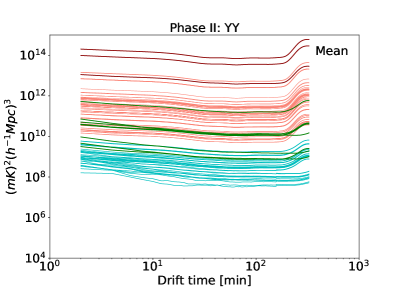
Figure 5: The mean HI power spectra are shown for the MWA data as a function of the drift time. The power spectra are computed using 5427 voxels for a given delay parameter $\tau$. The colour scheme is the same as in Figure 3.

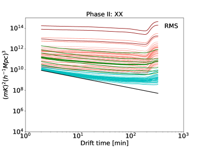
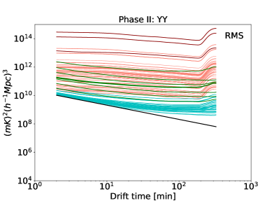
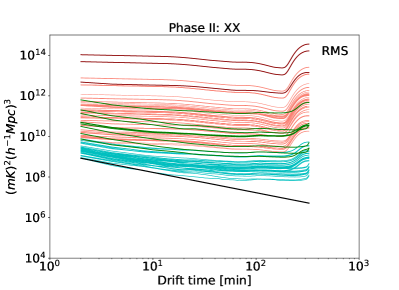
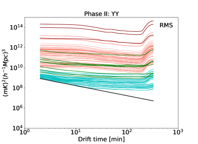
Figure 6: The top two panels show the RMS of the HI power spectrum of a voxel. The RMS is computed using 5427 voxels for a fixed $\tau$. The bottom two panels show the RMS after averaging the data over 100 randomly-chosen voxels which yields 54 sets which are used to compute the RMS. The mean power spectrum displayed in Figure 5 is left unchanged by this procedure. The colour scheme is the same as in Figure 3.

In Figure 5, we show the mean of the HI power spectrum as a function of the drift time. The mean HI power spectrum is computed by carrying out a weighted average over 5427 voxels for a fixed delay parameter $\tau$.

Figure 6 shows the RMS for a voxel and for a set of 100 voxels. The RMS of the power spectrum in the latter case is computed by first defining the power spectrum as weighted average over 100 randomly chosen voxels (for a fixed $\tau$) and then using these sets (54 sets) to compute the RMS. As noted above the mean is left unchanged by the second level of averaging as it only involves linear operations on the data. The lower envelope of the Figure 4 is plotted in the RMS plot for comparison.

Based on the discussion in the previous section, in which $g(t^{\prime}-t)$ was assumed to be unity, we can anticipate the behaviour of the the RMS of the HI power spectrum as a function of the drift time. Even for the shortest baselines we consider, the function $g(t^{\prime}-t)$ falls sharply after $t^{\prime}-t\simeq 30\,\rm min$. Therefore, we expect the following time dependence of the RMS: for a period of time for which $g(t^{\prime}-t)\simeq 1$, all the visibilities inside a pixel can be considered coherent. During this period, the RMS falls as $1/t$, for the reasons discussed in the previous section. The other limiting case occurs for $t^{\prime}-t$ such that $g(t^{\prime}-t)\simeq 0$. A pair of visibilities that satisfy this condition are incoherent. In this case, the RMS is expected to fall as $1/\sqrt{t}$. As the period of the drift scan far exceeds the coherence time scale of visibilities, the time dependence of visibilities is expected to make a transition from $1/t$ (all visibilities coherent inside a voxel) to $1/\sqrt{t}$ (all visibilities incoherent inside a voxel). Figure 6 shows that the departure of the RMS from $1/t$ time-dependence occurs after a drift time of nearly 20 minutes. As noted above, for a given delay parameter, the data from all the baselines is combined (using a weighted average which depends on the density of baselines in the UV plane) to yield the curves in Figure 6. The coherence time of the HI signal varies from a few minutes to nearly 30 minutes for the baselines used in our analysis. For the baseline distribution shown in Figure 1, the occupancy of a UV-pixel is skewed in the favour of shorter baselines, which explains the duration of the time of transition seen in Figure 6.

Finally, a comparison between the upper and the lower panels of Figure 6 shows that the decrement in the RMS from a single voxel to 100 randomly chosen voxels is nearly a factor of 10 for the cleanest delay parameters even though no such decrement is seen for the foreground-dominated modes. This result provides further proof that the clean modes are noise-dominated.

5.3 Two-dimensional power spectra and foreground wedge

Figures 5 and 6 adequately capture the time-dependence of the power spectra for different delay parameters and the separation of foreground-dominated modes from noise-dominated modes. To further analyze the complex structure of the signal in the Fourier domain, we show the signal in the usual $k_{\perp}\hbox{--}k_{\parallel}$ domain in Figures 7 and 8. In these figures, cylindrical averaging for a fixed $k_{\perp}=|{\bf k_{\perp}}|=\sqrt{k^{2}_{\perp 1}+k^{2}_{\perp 2}}$ is performed.

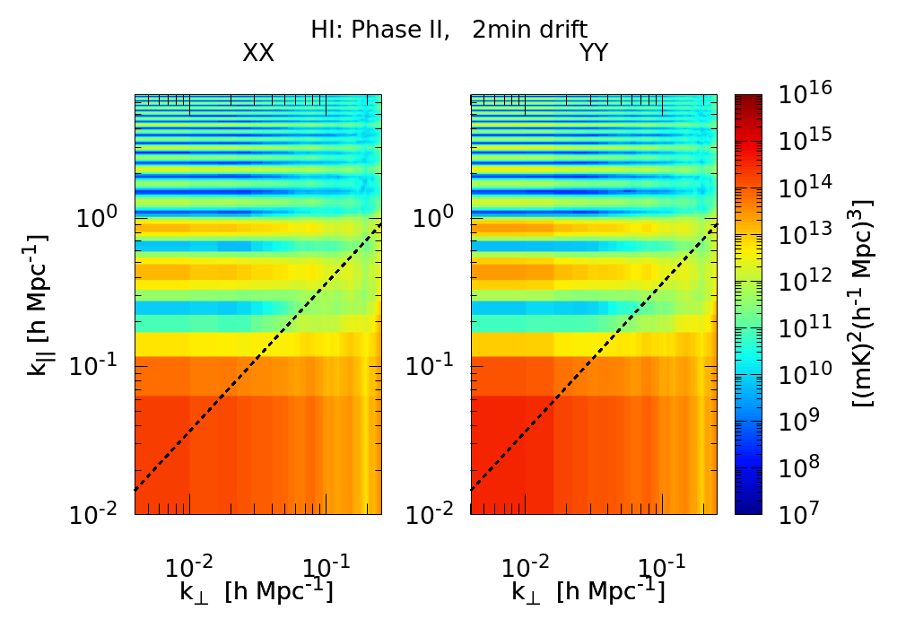
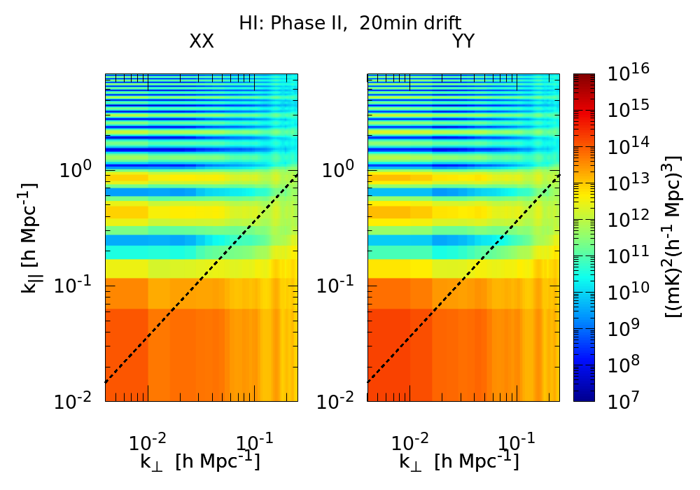
Figure 7: Two-dimensional power spectra are displayed for two fixed periods (2 and 20 minutes) of drift scans. The diagonal black line (plotted using the main lobe of MWA’s primary beam) separate the EoR window (the region above the line) from the foreground-dominated modes.

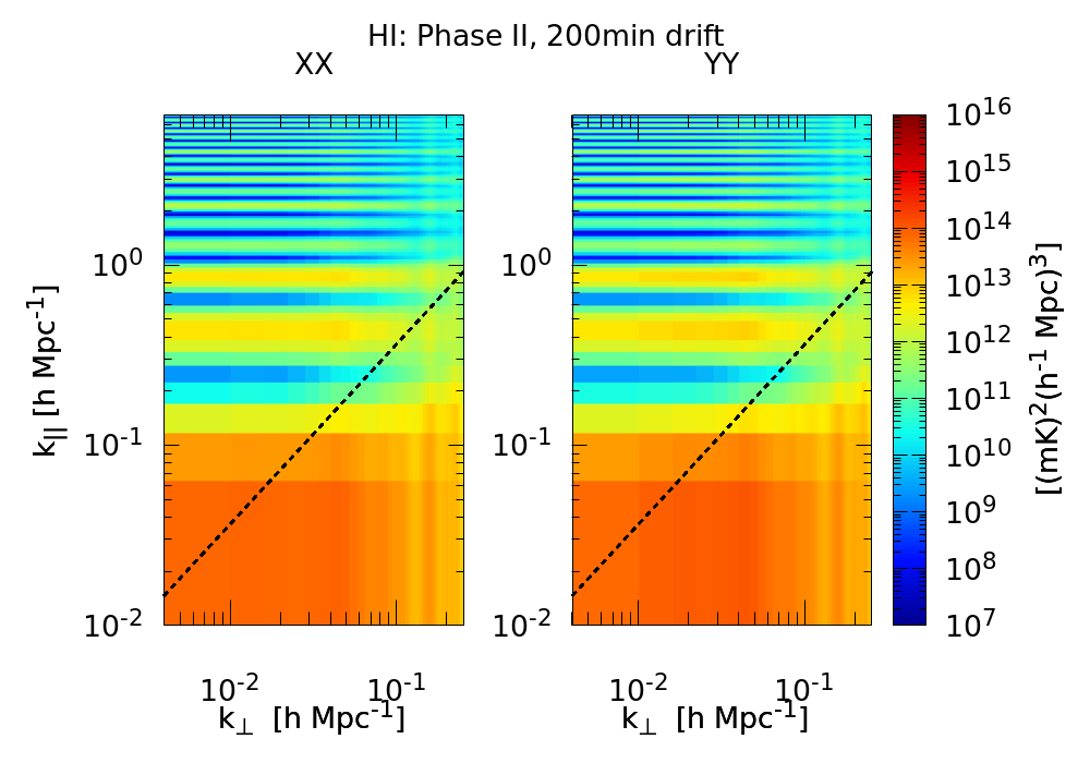
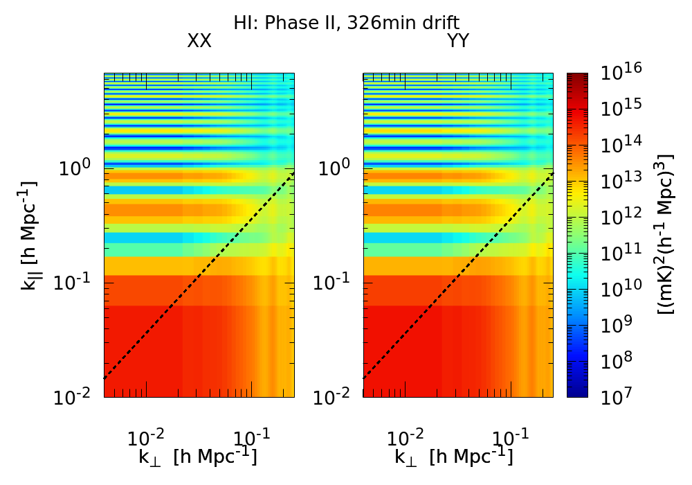
Figure 8: The 10-night combined data are displayed for 200 minutes and 326 minutes of drift scan.

We notice the characteristic features of delay space power spectra for MWA: foreground dominated wedge, cleaner EoR window, and the horizontal bands owing to the missing MWA spectral channels. As we already noted above, to reduce power leakage between $k_{\parallel}$ bins we apply Blackman-Nuttall window on visibilities before taking Fourier transform along the frequency axis (Eq. (2)). While the application of this window reduces the leakage and therefore the EoR window is cleaner, it thickens the horizontal bands.

The two-dimensional power spectrum should be viewed alongside Figure 5. Figure 5 shows the mean power spectrum computed by averaging over all the baselines of fixed $k_{\parallel}$ while the two-dimensional power spectra provide additional information for a given $|{\bf k_{\perp}}|$. The time dependence in both the cases is similar: as the drift scan time is increased from 2 minutes to 120 minutes, the EoR window gets cleaner by up to two orders of magnitude owing to the reduction of noise.

5.4 Foregrounds in drift scan

The separation of foreground-dominated modes from noise-dominated modes is a key requirement of the EoR science. The focus of this subsection is a discussion of the modes dominated by foregrounds with particular focus on drift scans but a part of the discussion is general enough to be applicable to the tracking observation also.

As shown in PS19, the behaviour of foregrounds in a drift scan could be markedly different from tracking observations (for another perspective on foregrounds in a drift scan see Shaw et al. (2014)). The coherence time scale of the HI signal is larger than that of the extragalactic point sources while it is comparable to the coherence time scale of the diffuse sources (modelled as a statistically homogeneous process in PS19). This means point sources can get uncorrelated in the process of extracting the HI signal.

We first consider Figure 3 which assumes $g(t^{\prime}-t)=1$. In this case, all the cross-correlations within a voxel are assigned equal weight. As the time of the scan is much larger than the coherence time scale of all the components, we expect partial de-correlation of point sources, the HI signal, and diffuse foregrounds. We notice a decline of power by nearly an order of magnitude in the foreground-dominated modes until late in the scan when Fornax A and the galactic plane start contributing significantly. This behaviour should be compared to that in Figure 5 in which $g(t^{\prime}-t)$ corresponds to the coherence function for HI signal for MWA. In this case, only a fraction of cross-correlations inside a voxel are carried out, which prevents the de-correlation of the HI signal. In this case, the decrement of the power in foreground dominated modes is also shallower because this process also prevents the de-correlation of diffuse foregrounds.

The complexity of the time-dependence of foregrounds in a drift scan is further revealed in Figures 7 and 8. In these figures, the power in Fourier modes in the plane of the sky is separated from the modes along the line of sight. Unlike Figure 5 which displays the power spectra averaged over all $|{\bf k_{\perp}}|$ for a given $k_{\parallel}$, Figures 7 and 8 show the results for a fixed $|{\bf k_{\perp}}|$. This allows us to discern the baseline dependence of the de-correlation process in a drift scan. From Figure 1 of PS19, we note that the de-correlation time of the HI signal varies from nearly 30 minutes to 5 minutes from the shortest to the longest baselines we consider in our study, $\sqrt{u^{2}+v^{2}}\simeq 20\hbox{--}300$.

Figure 7 clearly show the depletion of power in foreground-dominated modes as the drift time increases from 2 minutes to 20 minutes. However, this process does not cause the transition of any foreground-dominated mode to a noise dominated mode. This allows us to conclude that, for the data we analyse, drift scans don’t add any further information on the separation of foregrounds from the EoR window as compared to the tracking observation.

To get further evidence of the noise-dominated modes, we focus on Figure 6. This figure shows the RMS of the HI power spectrum decreases by the expected factor of nearly ten after the second level of averaging for the noise-dominated modes. However, this decrement is not seen for the foreground-dominated modes. Figures 3 and 4 also support this conclusion. This constitutes another diagnostic of the noise-dominated modes which are suitable for the EoR detection. We note that this method of comparing the RMS of the HI power spectrum using different sub-sets of data provides a suitable diagnostic for both the drift scan and tracking observations.

5.5 One-dimensional power spectrum

The information displayed in Figures 5 and 8 can be partially summarized with one-dimensional power spectrum defined as: $\Delta^{2}(k)=k^{3}P(k)/(2\pi^{2})$ with $k=\sqrt{{\bf k}_{\perp}^{2}+k_{\parallel}^{2}}$. For the EoR window, MWA baseline distribution gives $k_{\parallel}\gg|{\bf k}_{\perp}|$ and therefore the one-dimensional power spectrum can be computed by averaging over all ${\bf k}_{\perp}$ for a fixed $k_{\parallel}$ (it is partly the motivation of the choice of variables for Figure 5). The one-dimensional power spectrum as a function of time can be computed from Figure 5 (or Figure 8). The best results is obtained after nearly 200 minutes of the scan, as clearly seen in Figure 8. The contamination from Fornax A and the galactic plane prevents any further improvement. This also means that only 35 hours of data from a total of 55 hours is usable for our purposes.

Figure 8 shows that the largest scales in the EoR window that can be probed with MWA correspond to $k\simeq 0.2$$h~{}{\rm Mpc}^{-1}$, which gives us $\Delta^{2}(k)\simeq(1000~{}\rm mK)^{2}$ (for either XX or YY polarization). Figure 8 also shows that the cleanest modes are obtained for much smaller scales. For $k\simeq 1$$h~{}{\rm Mpc}^{-1}$, the one-dimensional power spectrum $\Delta^{2}(k)\simeq(1000~{}\rm mK)^{2}$, which is comparable to the value at larger scales.

The RMS of the HI power spectrum can be computed from Figure 6. It is based on 54 sets with each set obtained from weighted average over 100 voxels. This yields an RMS of $\simeq 10^{6}\,\rm(mK)^{2}$ for clean modes in the range $k\simeq 0.02\hbox{--}1$$h~{}{\rm Mpc}^{-1}$. The RMS estimate can be further improved by averaging over all the data for a fixed $\tau$ (this leaves the mean unchanged for reasons outlined in the foregoing) and then computing the RMS using bootstrapping (e.g. Kolopanis et al. (2019)).

We plot the power spectra for both the XX and YY polarizations in all the figures to emphasize the long-term system stability in a drift scan. Our calibration does not involve a polarized source so both the polarizations are assigned equal weight in the beginning of the scan. Our results show that no significant deviation emerges at the end of the scan. As the HI signal is unpolarized, the power spectra for the two polarizations can be added in quadrature to yield a further improvement in RMS by nearly a factor of $\sqrt{2}$.

5.5.1 Comparison with other HI power spectrum measurements

Our results can be directly compared to PAPER HI power spectra upper limits as it was also a drift scan experiment. PAPER was located in Karoo desert, South Africa at coordinates $30^{\circ}43^{\prime}17^{\prime\prime}$S, $21^{\circ}25^{\prime}42^{\prime\prime}$E. Its 2-meter antenna had a primary beam (FWHM) of nearly $50^{\circ}$. PAPER’s 64 antennas were placed in a 8x8 pattern. For the final results presented in Kolopanis et al. (2019), 6 of the antennas were flagged and only a subset of baselines were used for the power spectrum estimations. This subset consisted of 30-meter East-West baselines between adjacent columns and those staggered by one row (see Figure 2 of Kolopanis et al. 2019). The system temperature for the observational runs varied between 400–800 K in the frequency range. These data sets had a total bandwidth of 10 MHz with a channel width of 493 kHz, centered around six frequencies in the range 120–167 MHz. The power spectrum estimate was based on 135 days of observations, but only the data from 124 days was used for LST binning. The LST spanned the range $00^{\rm h}30^{\rm m}00^{\rm s}$ to $08^{\rm h}36^{\rm m}00^{\rm s}$. The data sets were initially binned with a time resolution 43 seconds. After the LST binning, they were further averaged with a top-hat filter in time which yielded a resolution of 938 seconds. With these instrumental parameters, the PAPER collaboration recently published the analysis of its final data products. Their upper limits on the HI power spectra at $z\simeq 8.13$ are: $\Delta^{2}(k)\simeq(1000~{}{\rm mK})^{2}$ at $k=0.2$$h~{}{\rm Mpc}^{-1}$and $(380~{}{\rm mK})^{2}$ at $k\simeq 0.32$$h~{}{\rm Mpc}^{-1}$(Kolopanis et al. 2019). Our upper limit at a comparable wavenumber and redshift is $\simeq(1000~{}{\rm mK})^{2}$, based on nearly 35 hours of MWA drift scan data.

While a more direct comparison between the performance of MWA and PAPER is harder, this allows us to note the following salient differences between the two interferometers and analysis pipelines: (a) the collecting area of MWA is nearly five times large, (b) PAPER baselines have a higher level of redundancy (section 3), (c) the time over which the visibilities are averaged is around 15 minutes for PAPER while it varies between a few minutes to nearly 30 minutes for MWA (for details of coherence time of these interferometers see PS19), (d) the drift time for PAPER is nearly 40 times larger as compared to our run, (e) cross-channel contamination is an important issue for MWA owing to missing channels which prevents a large fraction of modes from reaching the theoretical noise levels (Figure 3).

More recently, MWA collaboration published results from the analysis of its best tracking Phase I and Phase II data for three fields, EoR0, EoR1, and EoR2 for a range of redshifts and wavenumbers (Trott et al., 2020). The integration time on fields relevant to us varies from 27 to 38 hours which is comparable to the drift time in this paper. Even though a direct comparison is difficult owing to different modes of observations, our analysis is based on data that traverses between EoR0 and EoR1 fields, and therefore a comparison of our results with tracking data from EoR0 and EoR1 fields for the same redshift range and wavenumbers is justified.

For $z\simeq 8.2$ and $k\simeq 0.2$$h~{}{\rm Mpc}^{-1}$, the following upper limits were obtained by the MWA tracking observation: $(376~{}{\rm mK})^{2}$ (EoR0, 38 hours) and $(1166~{}{\rm mK})^{2}$ (EoR1, 27 hours). The limit we obtain in this paper is worse than the limit for the EoR0 field but marginally better than the limit for the EoR1 field. While the analysis of the tracking data reports the power spectrum for $k<0.7$$h~{}{\rm Mpc}^{-1}$, the primary results for the tracking data are more reliable for $k<0.4$$h~{}{\rm Mpc}^{-1}$(Trott et al., 2020). As noted above, our best results are obtained for the scale $k\simeq 1$$h~{}{\rm Mpc}^{-1}$. The analysis of the tracking data yielded the following upper limit for comparable scales: $\Delta^{2}(k)\simeq(2000~{}{\rm mK})^{2}$ (EoR0) and $\Delta^{2}(k)\simeq(3100~{}{\rm mK})^{2}$ (EoR1). Our results are an improvement over the tracking observation at this scale.

6 Summary and conclusion

The use of drift scan data to extract the HI power spectrum from high and low redshift data is an established method (e.g. Bandura et al. (2014); Kolopanis et al. (2019); Parsons et al. (2016); DeBoer et al. (2017)). Drift scans are expected to yield superior system stability which is one of the key requirements for the detection of the weak HI signal. In this paper we report the analysis of nearly 55 hours of publicly-available MWA Phase II drift scan EoR data. Our analysis is based on a novel method proposed in PS19, which is an extension of formalism given by Paul et al. (2014). We develop a pipeline which works in two modes: (a) noise testing: the aim of this mode is to test system stability by comparing the data power spectrum against uncorrelated noise as a function of the drift time, (b) HI mode: the HI power spectrum is computed in this mode. We summarize our main results and findings:

• Noise testing: Figures 3 and 4 show the main results. The figures demonstrate that the data agree with the behaviour of the thermal noise for a drift scan of nearly 4 hrs—the RMS falls as $1/t$ during this period. This provides reasonable proof that the system parameters (primary beam, bandpass) are stable over the duration of the scan. This test also allows us to estimate the mean system temperature during the scan, which is in agreement with the reported values.

• HI power spectrum: The HI power spectra as a function of time are shown in Figures 5 and 6. The two-dimensional plots (Figures 7 and 8) show the HI power spectrum in $k_{\perp}\hbox{--}k_{\parallel}$ plane for fixed drift times. These results are in line with the expectation that, for the clean modes, the RMS of the mean HI power spectrum initially falls as $1/t$ and then approximately as $1/\sqrt{t}$. This transition occurs when the drift time exceeds the coherence time of the HI signal. A comparison between the RMS computed from two different data subsets (Figure 6) also shows that the clean modes are noise-dominated and therefore suitable for EoR studies.

• Foreground-dominated modes: As shown in PS19, the point sources de-correlate on time scales much shorter than the HI signal, which means we expect some level of decrement in the power of the foreground-dominated modes even as the HI signal is extracted from the data. This is seen in Figures 5 and 6. However, it is difficult to draw a definite conclusion regarding the depletion of the power owing to the complicated nature of diffuse foregrounds.

The aim of this paper is to demonstrate a new method of analysing MWA drift scan EoR data. This method is particularly suited for repeated scans over a given field. We seek a proof of concept by testing system stability during a scan. We also compute the HI power spectrum.

The detection of the HI signal from the epoch of reionization remains a challenge. Given the weak HI signal buried under strong foregrounds and hundreds of hours of integration time needed to reduce the thermal noise to acceptable levels, it is perhaps imperative that multiple approaches are employed to understand and analyse the signal.

Data Availability

The data sets were derived from sources in the public domain (the MWA Data Archive: project ID G0031) at https://asvo.mwatelescope.org/.

Appendix A

Here we describe briefly the conversion of measured quantity (Eq. (1)) to the variables of the HI signal.

The parameters of the radio interferometer can be related to the Fourier variables of the HI signal as (e.g. Paul et al. (2016b) and references therein):

$$k_{\perp 1}=\frac{2\pi}{r_{0}}u_{0},k_{\perp 2}=\frac{2\pi}{r_{0}}v_{0},k_{\parallel}=\frac{2\pi}{|\dot{r}_{0}|}\tau.$$ (5)

Here $k_{\perp 1}$ and $k_{\perp 2}$ are the Fourier components on the sky plane while $k_{\parallel}$ lies along the line of sight. $r_{0}$ is the coordinate distance corresponding to the observed redshifted frequency $\nu_{0}$ and $\dot{r}_{0}=dr/d\nu$ at $\nu=\nu_{0}$.

The HI power spectrum can be written in terms of the visibility correlation function defined in Eq. (1) using:

$${P}_{\rm HI}(k)\simeq\frac{9|\dot{r}_{0}|r^{2}_{0}}{4\bar{I}^{2}_{0}B\Omega_{0}}|{\cal C}_{\tau}(\textbf{u}_{0},w_{0})|.$$ (6)

Here $\Omega_{0}=\frac{\lambda^{2}_{0}}{A_{\rm eff}}$ is the solid angle of the primary beam of MWA (the effective area of an MWA tile, $A_{\rm eff}=21.5\,\rm m^{2}$ at $\nu=154\,\rm MHz$; for details see Tingay et al. 2013) and $k=\sqrt{k^{2}_{\perp 1}+k^{2}_{\perp 2}+k^{2}_{\parallel}}$. $\bar{I}$ is the mean intensity of the HI signal. For a single polarization (either XX or YY correlation), $\bar{I}_{0}=k_{B}T_{B}/\lambda^{2}_{0}$, where $T_{B}$ is the mean HI brightness temperature and $k_{B}$ is the Boltzmann constant. For computing the mean intensity, we assume a neutral hydrogen fraction of 0.5 at $z=8.21~{}(154.24\text{MHz})$, which yields $T_{B}=12.6~{}\rm mK$. This gives us the normalization needed to convert visibility correlation from $(\rm JyHz)^{2}$ to $({\rm mK})^{2}(h^{-1}\rm Mpc)^{3}$, the units of the HI power spectrum:

$$\frac{9\lambda^{4}_{0}|\dot{r}_{0}|r^{2}_{0}}{4k^{2}_{B}B\Omega_{0}}=4.18\times 10^{-3}\frac{\text{$({\rm mK})^{2}(h^{-1}\rm Mpc)^{3}$}}{(\rm JyHz)^{2}}.$$ (7)

The factor of 9/4 in the normalization is specific to the MWA primary beam. We use Eqs. (7) and (6) for the analysis of the data.

References

- Bandura et al. (2014) Bandura K., et al., 2014, Canadian Hydrogen Intensity Mapping Experiment (CHIME) pathfinder. p. 914522, doi:10.1117/12.2054950
- Barry et al. (2019) Barry N., et al., 2019, ApJ, 884, 1
- Beardsley et al. (2016) Beardsley A. P., et al., 2016, ApJ, 833, 102
- Bowman et al. (2013) Bowman J. D., Cairns I., Kaplan D. L., Murphy T., Oberoi D., others 2013, PASA, 30, 31
- Bowman et al. (2018) Bowman J. D., Rogers A. E. E., Monsalve R. A., Mozdzen T. J., Mahesh N., 2018, Nature, 555, 67
- Choudhuri et al. (2016) Choudhuri S., Bharadwaj S., Chatterjee S., Ali S. S., Roy N., Ghosh A., 2016, MNRAS, 463, 4093
- Christiansen & Hoegbom (1969) Christiansen W. N., Hoegbom J. A., 1969, Radiotelescopes. Cambridge University Press
- Datta et al. (2010) Datta A., Bowman J. D., Carilli C. L., 2010, ApJ, 724, 526
- DeBoer et al. (2017) DeBoer D. R., et al., 2017, PASP, 129, 045001
- Dillon et al. (2015) Dillon J. S., et al., 2015, Phys. Rev. D, 91, 123011
- Eastwood et al. (2018) Eastwood M. W., et al., 2018, AJ, 156, 32
- Fan et al. (2006) Fan X., et al., 2006, AJ, 132, 117
- Furlanetto et al. (2006) Furlanetto S. R., Oh S. P., Briggs F. H., 2006, Phys. Rep., 433, 181
- Jacobs et al. (2013) Jacobs D. C., et al., 2013, ApJ, 776, 108
- Kolopanis et al. (2019) Kolopanis M., et al., 2019, ApJ, 883, 133
- Li et al. (2019) Li W., et al., 2019, ApJ, 887, 141
- McKinley et al. (2015) McKinley B., et al., 2015, MNRAS, 446, 3478
- McMullin et al. (2007) McMullin J. P., Waters B., Schiebel D., Young W., Golap K., 2007, in Shaw R. A., Hill F., Bell D. J., eds, Astronomical Society of the Pacific Conference Series Vol. 376, Astronomical Data Analysis Software and Systems XVI. p. 127
- Mertens et al. (2020) Mertens F. G., et al., 2020, MNRAS, 493, 1662
- Morales & Hewitt (2004) Morales M. F., Hewitt J., 2004, ApJ, 615, 7
- Morales & Wyithe (2010) Morales M. F., Wyithe J. S. B., 2010, ARA&A, 48, 127
- Nuttall (1981) Nuttall A. H., 1981, IEEE Transactions on Acoustics Speech and Signal Processing, 29, 84
- Offringa et al. (2015) Offringa A. R., et al., 2015, Publ. Astron. Soc. Australia, 32, e008
- Paciga et al. (2013) Paciga G., et al., 2013, MNRAS, 433, 639
- Parsons & Backer (2009) Parsons A. R., Backer D. C., 2009, AJ, 138, 219
- Parsons et al. (2012) Parsons A. R., Pober J. C., Aguirre J. E., Carilli C. L., Jacobs D. C., Moore D. F., 2012, ApJ, 756, 165
- Parsons et al. (2014) Parsons A. R., et al., 2014, ApJ, 788, 106
- Parsons et al. (2016) Parsons A. R., Liu A., Ali Z. S., Cheng C., 2016, ApJ, 820, 51
- Patil et al. (2017) Patil A. H., et al., 2017, ApJ, 838, 65
- Patwa & Sethi (2019) Patwa A. K., Sethi S., 2019, ApJ, 887, 52
- Paul et al. (2014) Paul S., et al., 2014, ApJ, 793, 28
- Paul et al. (2016a) Paul S., Patwa A. K., Sethi S., Dwarakanath K. S., 2016a, Detection of redshifted HI from the Epoch of Reionization using drift scans, MWA Proposal id.2016B-08
- Paul et al. (2016b) Paul S., et al., 2016b, ApJ, 833, 213
- Planck Collaboration et al. (2020) Planck Collaboration et al., 2020, A&A, 641, A6
- Pritchard & Loeb (2012) Pritchard J. R., Loeb A., 2012, Reports on Progress in Physics, 75, 086901
- Rogers & Bowman (2008) Rogers A. E. E., Bowman J. D., 2008, AJ, 136, 641
- Shaw et al. (2014) Shaw J. R., Sigurdson K., Pen U.-L., Stebbins A., Sitwell M., 2014, ApJ, 781, 57
- Shaw et al. (2015) Shaw J. R., Sigurdson K., Sitwell M., Stebbins A., Pen U.-L., 2015, Phys. Rev. D, 91, 083514
- Singh et al. (2018) Singh S., Subrahmanyan R., Shankar N. U., Rao M. S., Girish B. S., Raghunathan A., Somashekar R., Srivani K. S., 2018, Experimental Astronomy, 45, 269
- Tingay et al. (2013) Tingay S. J., Goeke R., Bowman J. D., Emrich D., others 2013, PASA, 30, 7
- Trott (2014) Trott C. M., 2014, Publ. Astron. Soc. Australia, 31, e026
- Trott et al. (2016) Trott C. M., et al., 2016, ApJ, 818, 139
- Trott et al. (2020) Trott C. M., et al., 2020, MNRAS, 493, 4711
- Wayth et al. (2018) Wayth R. B., et al., 2018, Publ. Astron. Soc. Australia, 35, 33
- van Haarlem et al. (2013) van Haarlem M. P., et al., 2013, A&A, 556, A2