Mask-ToF:  Learning Microlens Masks for
Flying Pixel Correction in Time-of-Flight Imaging

Abstract

We introduce Mask-ToF, a method to reduce flying pixels (FP) in time-of-flight (ToF) depth captures. FPs are pervasive artifacts which occur around depth edges, where light paths from both an object and its background are integrated over the aperture. This light mixes at a sensor pixel to produce erroneous depth estimates, which can adversely affect downstream 3D vision tasks. Mask-ToF starts at the source of these FPs, learning a microlens-level occlusion mask which effectively creates a custom-shaped sub-aperture for each sensor pixel. This modulates the selection of foreground and background light mixtures on a per-pixel basis and thereby encodes scene geometric information directly into the ToF measurements. We develop a differentiable ToF simulator to jointly train a convolutional neural network to decode this information and produce high-fidelity, low-FP depth reconstructions. We test the effectiveness of Mask-ToF on a simulated light field dataset and validate the method with an experimental prototype. To this end, we manufacture the learned amplitude mask and design an optical relay system to virtually place it on a high-resolution ToF sensor. We find that Mask-ToF generalizes well to real data without retraining, cutting FP counts in half.

1 Introduction

Large-scale image datasets such as ImageNet [15] and CIFAR [31, 32], in tandem with a boom in computational resources, drastically reshaped the field of image processing. In the depth domain, a similar trend [61, 8, 13] has recently made the mass-acquisition of high-quality depth maps a vital prerequisite for a range of 3D graphics and vision applications. These include human-centered tasks such as pose tracking [59, 29], action recognition [26, 51], and facial analysis [56], as well as scene-understanding problems including mapping [19], segmentation [14], and object reconstruction [70, 10, 75]. While methods look to captured depth datasets for ground truth, the devices used to capture them are subject to a slew of error sources which, if not addressed, can hurt task performance and generalizability.

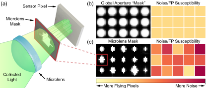
Figure 1: (a) 3D visualization of a microlens mask selectively blocking light entering a sensor pixel. (b) The equivalent mask pattern for a global aperture setup, all sensor pixels equally susceptible to FPs. (c) A learned mask pattern with spatially multiplexed noise/FP susceptibility.

One of many approaches to depth acquisition is passive sensing: exploiting parallax cues to infer distances solely from input monocular [66, 41, 18] or multiview [24, 27, 73] images. These methods can use standard RGB cameras for data acquisition, but struggle with textureless regions and complex geometries [63, 36]. Active sensing approaches tackle this challenge by first sending out a known illumination into the scene and reconstructing depth with the help of the returned light. These include structured light methods such as active stereo, where spatially patterned light is projected into the scene to aid in the stereo feature matching process [1]. While being robust to textureless scenes, their accuracy is fundamentally limited by illumination pattern density and sensor baseline, resulting in a bulky camera form-factor. Some of the most successful active depth sensing methods are time-of-flight (ToF) approaches, where depth is estimated from the travel time of light leaving and returning to the device. Direct ToF systems such as LiDAR send out individual laser pulses and measure their time to return using time-resolved sensors such as avalanche photo diodes [12]. These can provide high-accuracy and long-range depth estimates, but use a scanning approach to collect data, leading to poor depth completeness and/or expensive sensor array systems. In contrast, amplitude-modulated continuous wave (AMCW) ToF cameras, the focus of this paper, flood-illuminate a scene with periodic amplitude-modulated light and estimate the phase shift of returned light to infer depth. These devices do not need to time-resolve captured light like their direct ToF counterparts, and so can rely on an easy-to-manufacture CMOS sensor array to produce complete depth maps at a high framerate. This, when combined with their small sensor-illumination baseline, makes AMCW ToF cameras compact and affordable, and has led to their widespread adoption in the vision community. Devices such as those in the Microsoft Kinect series have subsequently helped create community-made freely-available scene understanding benchmarks that lower the barrier of entry for 3D vision research [64, 2].

Although they promise to democratize low-cost dense depth imaging, AMCW ToF methods are still subject to fundamental limitations of the sensing process: noise from ambient light, photon shot, phase wrapping, multipath interference (MPI), and flying pixels (FPs) [16]. There has accordingly arisen a large body of work in computational post-processing methods to address these issues; methods concerning depth denoising [17, 74], phase unwrapping [35], and MPI correction [42]. Contrastingly, while confidence-based methods [55] are able to identify flying-pixels, rectifying them — recovering the depth of their corresponding chief ray — has remained a great challenge.

FPs are formed when light from both an object and its background reaches the same sensor pixel, generating a mixed depth measurement. These often appear to be floating in empty space in the resultant point cloud, hence flying pixels. Computationally unmixing these FPs often leads to edge blur or severe artifacts [72]. As they originate in the optical pipeline, artifacts of the light collection process by the main lens, we argue that an effective strategy to mitigate them should also start in the optical pipeline. Unfortunately, a direct masking approach, such as simply reducing aperture size to block stray light paths, is not efficient for overall light throughput, and so significantly lowers SNR.

With Mask-ToF we learn a microlens amplitude mask, allowing us to generate per-pixel aperture configurations with spatially-varying susceptibility to noise and FPs, as shown in Figure 1. We train an encoder-decoder network which learns to aggregate this spatial information and leverages mask structural cues to produce refined depth estimates. We then backpropagate this net’s loss to jointly learn high-level mask patterns. We photolithographically manufacture the learned mask, and virtually place it on the sensor with a custom optical relay system to validate Mask-ToF on real-world data. In the future, we expect this mask can be fabricated directly on the camera sensor in a similar manner to a polarization sensor [47], preserving its form factor.

In summary, we make the following contributions:

• We develop a differentiable AMCW ToF image formation model, including sub-aperture light transport.

• We incorporate sub-aperture masking and a refinement network into this framework and learn an optimal mask structure through a patch-based gradient descent approach from synthetic data.

• We test the masks in simulation, evaluating on overall error and FP reduction, then manufacture them and construct an experimental setup to validate the proposed method on real data.

2 Related Work

Depth Imaging.  There exists a wide body of work in both passive and active methods for depth imaging. The former operates with only passive depth cues, such as parallax [24, 5, 46] and defocus [66, 66], to infer depth. These methods exhibit diminished accuracy for textureless scenes with few visual cues and complex geometries with ambiguous cues [63]. Active methods overcome this challenge by sending out a known illumination pattern into the scene and using the returned signal to help reconstruct depth. While structured light approaches rely on this illumination to improve local image contrast [58, 1], ToF imaging uses the travel time of light itself to measure distance [23, 60]. This sensing approach allows for compact illumination-sensor setups and does not hinge on ambiguous visual cues.

ToF Imaging.  ToF imaging can be further categorized into direct and indirect methods. Direct ToF devices such as LiDAR send out pulses of light, scanning over a scene and directly measuring their round-trip time via avalanche photodiodes [12, 50] or single-photon detectors [45, 22]. While accurate and long-ranged, these systems can produce only a few spatial measurements at a time, resulting in sparse depth maps [40]. Furthermore, their specialized detectors are orders of magnitude more expensive than conventional CMOS sensors. AMCW ToF imaging, a representative indirect ToF method, instead floods the whole scene with periodically modulated light and infers depth from phase differences between captures [20, 34]. These captures can be acquired with a standard CMOS sensor, making AMCW ToF cameras an affordable solution for dense depth measurement. Ultimately, all these devices integrate light over an aperture and are thus susceptible to FPs [55, 57].

Depth Reconstruction Methods.  Depth cameras are all subject to erroneous measurements, which has led to a wide array of work in robust depth reconstruction algorithms. Some approaches attempt to learn a direct mapping between noisy and clean 3D points [44, 49], though they are limited in their scope and scalability as they contend with graph operations on unstructured point cloud data [53, 54]. Correlation between color and depth has also been used to smooth noisy depth estimates and enforce view consistency [30, 38], though these approaches often blur object edges, producing more FPs. Confidence-based methods for ToF [55, 17] on the other hand can detect FPs as unreliable measurements, but lack the context needed to determine if they belong to an object, background, or intermediate depth. Mask-ToF resolves this problem with a two-stage, generalizable approach that joins reconstruction with the optical pipeline; where a spatially varying amplitude mask encodes the information needed to correct these flying pixels.

Masks for Computational Imaging.  Masks enable an imaging system to directly modify the point spread function (PSF) of input light, densely encoding information about the scene that can be computationally recovered post-capture. Amplitude masks can only attenuate light, yet have a wide range of applications including light-field [43], lensless [4], x-ray [52], high-speed [39], and spectral imaging [3]. Phase masks can allow for finer manipulation of PSFs [11], and may be of interest in future masked ToF projects, but are prohibitively expensive to manufacture at a micro-scale resolution. In this work we learn an occlusion mask with spatially varying microlens apertures, encoding scene geometric information in AMCW ToF measurements to help correct FPs during reconstruction.

End-to-End Design of Optics and Computation.  Conventional imaging systems are designed in a sequential manner: first develop the optical and sensor stack in isolation, driven by compartmentalized metrics, then delineate an image processing pipeline [69]. Recently, a new paradigm of jointly optimizing optics and reconstruction has emerged, where all stages are jointly optimized in the design phase. These hold promise for applications in extended depth-of-field [62], microscopy [48], monocular depth [9], HDR [67], hyperspectral [6], and transient [68] imaging. Inspired by these works, Mask-ToF uses a differentiable ToF simulator to jointly learn an optimal mask pattern and train a depth refinement network to produce high SNR, low FP depth maps.

3 Image Formation

Before introducing our proposed method, we review the fundamentals of AMCW ToF imaging; for details see [33].

Pinhole Model.  Correlation ToF cameras flood-illuminate the scene with an amplitude-modulated light signal

$$p(t):=\alpha\cos(\omega t)+\beta.$$ (1)

Here $\omega$ is a modulation frequency, $\alpha$ is amplitude, and $\beta$ is signal bias. Under a pinhole camera model this modulated light is perfectly reflected by an object and captured by the ToF camera after travel time $\tau$. The measured signal

$$\tilde{p}(t-\tau)=\tilde{\alpha}\cos(\omega t-\phi)+\tilde{\beta},\quad\phi=\omega\tau$$ (2)

is effectively $p(t)$ with attenuated amplitude $\tilde{\alpha}$, shifted bias $\tilde{\beta}$, and an introduced $\tau$-dependent phase shift $\phi$.

The camera then correlates $\tilde{p}(t-\tau)$ with an identically modulated reference signal $r(t)=\cos(\omega t+\psi)$ to produce

$$C(\psi)=\int_{0}^{T}{\tilde{p}({t-\tau})r(t)dt}\;\approx\;\frac{\tilde{\alpha}}{2}\cos(\phi+\psi),\\$$ (3)

for integration time $T\gg\tau$. By sampling correlation values $C(\psi)$ at four different phase offsets $\psi\!=\!\left[0,\,\pi/2,\,3\pi/2,\,\pi\right]$, we can extract the measured signal’s true phase $\phi$ from

$$\phi=\arctan\left(\frac{C(\pi)-C(\pi/2)}{C(0)-C(3\pi/2)}\right)+2\pi n.\quad n\in\mathbb{N}.$$ (4)

This arctangent, however, introduces a $2\pi n$ phase ambiguity for depths $z\geq\lambda=c/2\omega$, halved for the round-trip distance and with $c$ being the speed of light. To estimate this factor $n$ we can use a phase unwrapping algorithm [35], which typically solves instances of Equation (4) for multiple modulation frequencies $\omega$ and disambiguates $\phi$ via Euclidean division [71]. This estimate is ultimately converted to depth as $z=\phi c/4\pi\omega$.

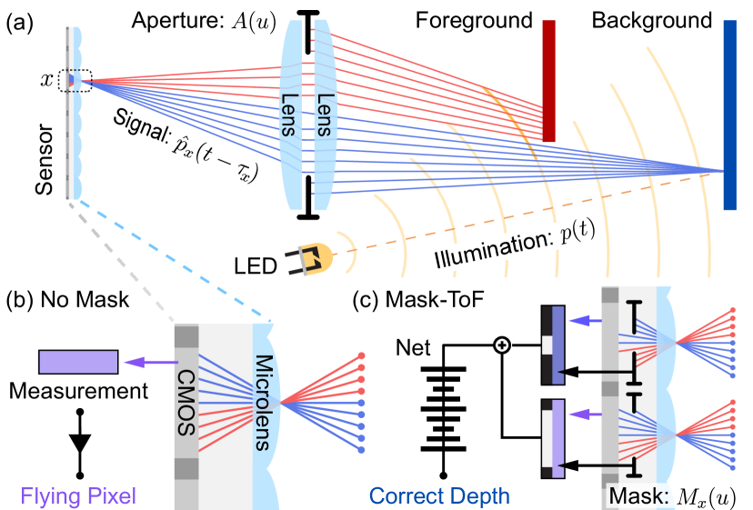
Figure 2: (a) ToF measurement at an object edge. (b) Without a mask, signals mix in unknown quantities to produce a flying pixel. (c) Mask-ToF can use surrounding pixel values and mask structure to disambiguate this measurement.

Lens Model.  In a practical camera system, to increase light throughput, we use a lens to focus light incident on an aperture plane $\mathcal{U}$ to a sensor pixel $x$; for simplicity we assume a 2D model. We thus rewrite the image formation model as

$$\hat{p}_{x}(t-{\tau_{x}})=\int_{u\,\in\,\mathcal{U}}A(u)\tilde{p}_{x}(t-{\tau_{x}}-\tau_{u})du,$$ (5)

where $\hat{p}_{x}$ is the measurement at pixel $x$, $A(\cdot)$ is a binary aperture function, $u\in\mathcal{U}$ is the aperture coordinate, and $\tau_{u}$ is an additional time-of-flight term incurred by the residual path length. $\tilde{p}_{x},\tau_{x}$ refer to Equation (2) evaluated for a ray connecting through point $u$ to $x$. The length of this ray is

$$d_{u,x}=\sqrt{(r-u)^{2}+f^{2}}+\sqrt{z^{2}+(\frac{xz}{f}+u)^{2}},$$ (6)

where $f$ is the focal length of the lens, $z$ is the depth of the scene point, and $r$ is the lens radius. For a typical AMCW ToF camera, with operating range $z\gg r$ and modulation frequency $\omega=\mathcal{O}(10^{8}\mathrm{Hz})$, the phase contribution from the residual distance term $\delta_{u,x}=d_{u,x}-d_{0,x}$ is negligible. We thus discard the corresponding time-of-flight term $\tau_{u}$, and approximate the image formation model as

$$\hat{p}_{x}(t-{\tau_{x}})\approx\int_{u\,\in\,\mathcal{U}}A(u)p_{x}(t-{\tau_{x}})du.$$ (7)

Flying Pixels.  While for an unobstructed point $z$ this image formation is adequate, an edge case arises for points at a depth discontinuity. Suppose there is a single pixel on the sensor whose chief ray ($u=0$) comes from an $x$ near an object edge, see Figure 2. This would mean that for part of the aperture coordinates, $\mathcal{U}^{F}$, we would receive unfocused light rays from the foreground object, with travel time $\tau^{\prime}$, while the other rays passing through $\mathcal{U}^{B}=\mathcal{U}\setminus\mathcal{U}^{F}$ would have the intended travel time $\tau$. The received signal would similarly consist of a mix of both foreground $\hat{p}^{F}_{x}(t-\tau^{\prime}_{x})$ and background $\hat{p}^{B}_{x}(t-\tau_{x})$ measurements

$$\hat{p}(t-\tau):=\hat{p}^{F}(t-\tau^{\prime})+\hat{p}^{B}(t-\tau)$$

$$\Rightarrow\> \hat{p}(t-\tau)=\tilde{\alpha}\cos(\omega t-\phi)+\tilde{\alpha}^{\prime}\cos(\omega t-\phi^{\prime})+\tilde{\beta}+\beta^{\prime},$$

$$\phi=\omega\tau,\;\phi^{\prime}=\omega\tau^{\prime}$$

$$\Rightarrow\> \hat{\phi}=\arctan\left(\frac{\tilde{\alpha}\sin(\phi)+\tilde{\alpha}^{\prime}\sin(\phi^{\prime})}{\tilde{\alpha}\cos(\phi)+\tilde{\alpha}^{\prime}\cos(\phi^{\prime})}\right),$$ (8)

where $\hat{\phi}$ is the measured phase shift of this mixed signal. Solving Equation (4) returns an incorrect depth $\hat{z}$ somewhere between the foreground and background depths.

Aperture-Masked ToF Image Formation.  It might seem that a simple solution to the above flying pixel problem is just to reduce the aperture size. In the extreme case where $A(u)=0,\forall u>0$, we retain only the chief ray and so have no mixed measurements. Unfortunately, this also leads to poor light efficiency, which lowers the system’s SNR as it becomes more susceptible to photon shot. We provide a detailed discussion of this fundamental SNR/FP tradeoff in the Supplemental Document. To better maintain light throughput, we can selectively block light paths by applying a spatially-varying microlens amplitude mask $M_{x}(u)$ to the image plane. The model from Equation (7) thus becomes

$$\hat{p}_{x}(t-\tau_{x})=\int_{u\,\in\,\mathcal{U}}M_{x}(u)A(u)p_{x}(t-{\tau_{x}})du.$$ (9)

One could imagine an ominscient mask $M_{x}(u)=0$ for $u\in\mathcal{U}^{F}$, else $M_{x}(u)=1$. This would remove unfocused foreground light and preserve all other light paths, perfectly correcting FPs with high SNR. Unfortunately, such a mask could only work for a single scene, and we would need to know that scene beforehand to design it. Instead, with the derivations above, we can form a differentiable framework for AMCW ToF image formation and use gradient descent to learn a single generalizable mask pattern. We describe this approach in the following section.

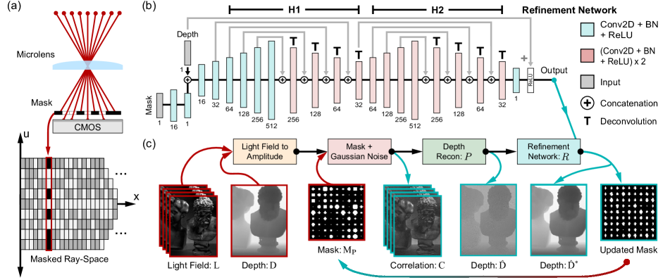
Figure 3: (a) Our microlens mask enables spatially-varying aperture coding in the angular-spatial domain. (b) The refinement network $R$, with skip connections in gray, which aggregates mask and coded depth information to produce a reduced FP output. (c) Stages of the differentiable simulation pipeline, from input light-field data to output refined depth.

4 Learning to Mask Flying Pixels

Mask Intuition. Before we outline how to learn a mask, it’s important to intuit why a static mask could help correct FPs in the first place. With a global aperture, shown in Figures 1 and 2 (b), all pixels are equally susceptible to FPs; if one sensor pixel returns an FP, likely so will its neighbors. The addition of spatially variable susceptibility via a microlens mask, shown in Figures 1 and 2 (c), means this is no longer the case. A sensor pixel with a wide effective aperture can be trusted with regards to noise statistics but is likely to return FPs when near an object boundary. Contrastingly, a neighboring pixel with a narrow aperture will likely produce noisier measurements, but be less affected by depth discontinuities. By aggregating information in pixel neighborhoods, we can effectively use wide aperture pixels to denoise local measurements, and narrow aperture pixels to de-flying-pixel them. This means a Mask-ToF approach critically needs not only a mask, but also a method to decode the information encoded by the mask.

From Light to Time-of-Flight.  Given ground truth depth, we can simulate ToF measurements via Equation (2) without distinguishing between light rays. However, to apply the mask $M_{x}(u)$ as in Equation (9), we also need access to the aperture plane $\mathcal{U}$. We thus discretize the image formation model and use light fields [37] as a natural parametrization

$$\hat{p}_{u,x}(t-\tau_{x})=\sum_{u\,\in\,L}M_{x}(u)A(u)p_{x}(t-{\tau_{x}}).$$ (10)

Here $\hat{p}_{u,x}$ is our ToF signal, a sum over sub-aperture views $u$ in the light field $L$, discretized now in both $x$ and $u$. As the number of sub-aperture views $|L|\rightarrow\infty$ we converge on the form of Equation (9), though in practice $|L|$ governs mask resolution and is limited by manufacturing constraints.

Tensor Image Model.  Rather than operate on $\hat{p}_{u,v,x,y}$, in 3D space we swap to a tensor view of simulation, as visualized in Figure 3 (c). We start with a depth map $\mathrm{D}\in\mathbb{R}^{H{\times}W}$, which we convert to phase array $\Phi$, and with the light field tensor $\mathrm{L}$ simulate $4{\times}|\mathrm{L}|$ correlation images $C_{0,0}-C_{3,|L|}$. One for each of four phase shifts $\psi$ and sub-aperture arrays $\mathrm{L}_{u}\in\mathrm{L}$. These are individually masked by $\mathrm{M}_{u}$, and the views are averaged to produce 4 final correlation images $\mathrm{C}_{\psi}$, subject to simulated noise $\eta_{\psi}$. This process is summarized in Equation (4).

$$\mathrm{C}_{\psi,u}=\mathrm{L}_{u}\odot(0.5+\cos(\Phi+\psi))\frac{gT}{\pi},\quad\Phi=\frac{4\pi\omega}{c}\mathrm{D}$$

$$\mathrm{C}_{\psi}=\eta_{\psi}+\frac{1}{|\mathrm{L}|}\sum_{u}\mathrm{M_{u}}\odot\mathrm{C}_{\psi,u}$$

$$\eta_{\psi}\sim\mathrm{uniform}(a,b)\cdot\mathcal{N}^{H{\times}W}(\mu,\sigma^{2}).$$ (11)

Here $g$ is sensor gain, $T$ is integration time, $H{\times}W$ is the sensor size, and $\odot$ denotes element-wise multiplication. The noise constants $a,b,\mu,\sigma$ are chosen empirically. At high photon counts, Poisson and Skellam [7] noise can be well approximated by scaled Gaussian noise, thus $\eta$ generalizes many expected sources of ToF noise [21] while maintaining simulation differentiability.

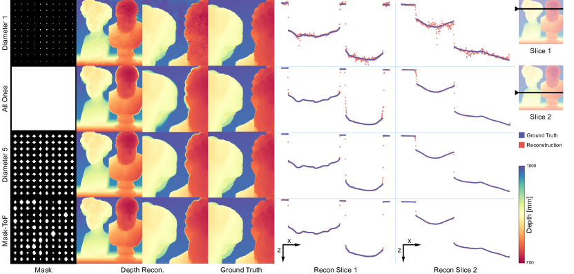
Figure 4: Comparison of optimized and naïve mask design results on simulated test data, with zoomed view of reconstruction and ground truth regions. Slices of the depth maps are plotted to help visualize flying pixels and noise susceptibility.

Depth Reconstruction. Using Equation (4) we generate an estimated depth map $\mathrm{\hat{D}}$ from the four masked correlation images $\mathrm{C}_{\psi}$. We implement this as a differentiable function $\mathrm{\hat{D}}=P(\mathrm{C})$ with automatic gradient evaluations. This grants us flexibility as we can swap $P(\mathrm{C})$ for other depth estimation methods, such as the discrete Fourier transform, if needed. To process the information embedded in these measurements by the microlens mask, we propose a refinement network $R$, illustrated in Figure 3 (b). $R$ is a residual encoder-decoder model, inspired by the hourglass architecture from [73], which takes as input $\mathrm{\hat{D}}$ and $\mathrm{M}$ and outputs

$$\mathrm{\hat{D}^{*}}=R(P(\mathrm{C}),\mathrm{M})=\max(0,\mathrm{\hat{D}}+\mathrm{\hat{D}^{R}}),$$ (12)

where $\mathrm{\hat{D}^{*}}$ is the refined depth map and $\mathrm{\hat{D}^{R}}$ is a learned residual depth which when added to $\mathrm{\hat{D}}$ serves to correct the now spatially multiplexed effects of noise and FPs. As Equation (4) does the initial depth calculation, $R$ does not have to learn how to generate depth from phase, and can be made significantly more lightweight than a typical deep reconstruction network. This helps $R$ to quickly learn high-level depth and mask features, and generalize well to arbitrary scenes where raw phase data might significantly differ from the training set. The sequential depth estimation and refinement approach also allows us to naturally exploit calibration procedures [29] implemented by the sensor manufacturer. We can feed real depth data directly into $R$ without having to retrain and learn calibration offsets.

Loss Functions.  For training, we opt for a combined loss

$$\mathcal{L}=\frac{1}{HW}\sum_{i}\left(w_{L}\mathcal{L}_{S}(\mathrm{\hat{D}^{*}_{i}},\mathrm{D_{i}})+w_{C}\mathcal{L}_{C}(\mathrm{\hat{D}^{*}_{i}},\mathrm{D})\right),$$

$$\mathcal{L}_{S}(\mathrm{\hat{D}^{*}_{i}},\mathrm{D_{i}})=\left\{\begin{array}[]{ll}|\mathrm{\hat{D}^{*}_{i}}-\mathrm{D_{i}}|-\delta/2&\text{ if }|\mathrm{\hat{D}^{*}_{i}}-\mathrm{D_{i}}|\geq\delta\\ (\mathrm{\hat{D}^{*}_{i}}-\mathrm{D_{i}})^{2}/2\delta&\text{ else },\end{array}\right.$$ (15)

$$\mathcal{L}_{C}(\mathrm{\hat{D}^{*}_{i}},\mathrm{D})=\min_{j}\|\mathrm{proj}(\mathrm{\hat{D}^{*}_{i}})-\mathrm{proj}(\mathrm{D_{j}})\|,$$ (16)

where $i,j\in\{0,...,HW-1\}$ are enumerative indices. Smooth L1 loss $\mathcal{L}_{S}$ helps enforce local smoothness in the reconstructed depth map, controlling the Gaussian noise $\eta$ while being less sensitive to depth outliers. To penalize these outliers, we add a Chamfer loss term $\mathcal{L}_{C}$. It considers the projected points $\mathrm{proj}(p)$, which we produce by concatenating sensor coordinates $x,y$ to the corresponding depth values $z$, and penalizes points based on their distance to the nearest ground truth point. FPs, which exist in the empty space between foreground and background depths with no close neighbors, are thus heavily penalized. We balance these losses with weights $w_{L}$ and $w_{C}$.

Patch-based Training.  We can propagate the gradient of this loss through the differentiable framework above all the way to the mask $\mathrm{M}$, however, learning an unconstrained $\mathrm{M}$ proves computationally burdensome. We thus restrict $\mathrm{M}$ to be an $m{\times}n$ tiling of a mask patch $\mathrm{M_{P}}$ and learn $\mathrm{M_{P}}$ instead, adopting a patch-based stochastic gradient descent approach. We sample a batch of random patches from the input light field and ground truth depth, and update $\mathrm{M_{P}}$ and $R$ based on the patch loss. This effectively exponentially increases the number of available samples for training, allowing us to rely on a relatively small light field dataset. As $R$ is fully convolutional, it is invariant to input shape, and so this patch training generalizes well to the full-sized images.

5 Synthetic Assessment

Implementation.  Our network $R$ is trained on patches of size $80{\times}80{\times}9{\times}9$ sampled from $512{\times}512{\times}9{\times}9$ synthetic light field data. This data, sourced from [25], contains $9{\times}9$ sub-aperture views per image pixel, and a total of 16 light fields. The full-sized evaluation masks are constructed by an $8{\times}8$ tiling of the center $64{\times}64$ area of the learned mask $\mathrm{M_{P}}$, reducing edge artifacts from training. Noise parameters $a,b,\mu,\sigma$ from Equation (4) are set to 0.75, 1.25, 0, 3; empirically matched to real recorded ToF samples. We set sensor gain to $g=20$ and integration time to $T=1$ ms.

The ADAM optimizer was used for training [28], with an initial learning rate of $0.004$ for the refinement network $R$ and $0.1$ for the mask $\mathrm{M_{P}}$. We halve both rates every 80 epochs. $\mathrm{M_{P}}$ is not updated for the first 70 epochs of training, as these epochs tend to be extremely noisy, the convolutional layers of $R$ having not yet learned high-level structures [76]. Through empirical study we found weights $w_{L}=100$ and $w_{C}=0.08$ to effectively balance the differing scales of Chamfer and smooth L1 loss in Equation (4). We leave $\delta$ as the default $\delta=1$. The network contains 19 million learnable parameters, 1 million of which are the amplitude mask, and is trained for 3 hours on a single Nvidia Tesla V100. Inference time for a single 512${\times}$512 image is $\approx 8$ ms. Code and trained models will be made available.

Ablation Study.  We quantify the effects of architecture design choices in a series of ablation experiments, summarized in Table 1. Here, Proposed is our final network $R$, and Chamfer Only$/$L1 Only are tests where we train $R$ using only the respective loss function. In the Half modification we remove the first hourglass, H1, while in Big we double intermediate channel counts in $R$. These help gauge if the network can be simplified or requires increased parametrization. The Global modification adds another global channel, implemented by duplicating H1 with increased stride lengths and concatenating the new signal at the input to H2, to test if the network can be improved by aggregating more non-local information. The No Mask tests the effect of training $R$ on only depth data, without mask input. Lastly, ToFNet is a reimplementation of the ToFNet architecture from [65]. We train it until convergence with weighted L1 and TV loss as suggested in the original work, and fine-tune the learning rate to our data.

Ablation	RMSE $\downarrow$	MAE $\downarrow$	Thresh 3mm $\downarrow$	Thresh 15mm $\downarrow$
Mask-ToF	5.166$/$7.115	1.281$/$1.278	5.052$/$4.397	1.178$/$1.120
Chamfer Only	6.459$/$7.913	1.992$/$1.930	10.91$/$9.878	1.457$/$1.330
L1 Only	5.216$/$7.127	1.284$/$1.293	5.024$/$4.426	1.214$/$1.194
Half	5.489$/$7.432	1.356$/$1.367	5.247$/$4.647	1.391$/$1.373
Big	5.432$/$7.169	1.514$/$1.482	6.351$/$5.439	1.369$/$1.284
Global	5.427$/$7.310	1.407$/$1.393	5.488$/$4.716	1.363$/$1.307
No Mask	5.482$/$7.353	1.410$/$1.398	5.284$/$4.664	1.369$/$1.303
ToFNet	11.42$/$12.19	5.120$/$5.038	42.36$/$42.82	5.316$/$4.964

Table 1: Quantitative ablation results (train$/$test) for changes to network $R$ or training procedure. Thresh Xmm is a threshold metric denoting the percentage of points further than X millimeters from ground truth depth.

Mask	RMSE $\downarrow$	MAE $\downarrow$	Thresh 3mm $\downarrow$	Thresh 15mm $\downarrow$
Diam. 1	9.412$/$8.293	5.203$/$4.576	46.31$/$46.549	6.647$/$4.345
All Ones	9.227$/$12.58	2.470$/$2.814	9.712$/$10.45	3.118$/$3.558
Diam. 5	6.512$/$8.732	1.718$/$1.753	7.377$/$6.552	1.585$/$1.582
Mask-ToF	5.166$/$7.115	1.281$/$1.278	5.052$/$4.397	1.178$/$1.120

Table 2: Quantitative comparison (train$/$test) of mask-aided ToF recovery. 4 images (greek, pillow, pens, tower) of 16 withheld for testing.

We validate the proposed architecture of the network $R$ with the results in Table 1. Specifically, the proposed method wins in all categories compared to the Big and Half, suggesting it is adequately parametrized. The lack of improvement from Global also suggests that the network $R$ is sufficiently utilizing non-local information. Chamfer Only and No Mask both lead to lackluster performance, emphasizing the value of the L1 regularization term and mask comprehension, respectively. Although we see close results for L1 Only, the addition of Chamfer loss does lead to a reduction in outliers, expressed in RMSE and threshold metrics. ToFNet shows overall worse performance than our Baseline refinement architecture, with the network learning to reconstruct a smooth depth map, however not learning to remove flying pixels. This is possibly due to its significantly wider scope; lacking a skip layer to the output, it must learn to reconstruct depth from raw phase measurements.

Analysis of Mask Patterns.  Mask-ToF contains a feedback loop: a change in the mask structure of $\mathrm{M_{P}}$ necessitates an update to the refinement network $R$, which itself alters the propagated loss gradient and changes the structure of $\mathrm{M_{P}}$. Thus, to avoid local minima, we test a broad set of both human-selected and randomly generated initial masks including: various diameters of circular aperture, Gaussian and Bernoulli noise, randomly oriented barcode structures, and several multiplexed designs. A full discussion of mask patterns is available in the Supplemental Document.

We compare the final optimized mask against the best hand-crafted (naïve) initializations to validate our proposed end-to-end optimization method. For a fair comparison, we fine-tune the refinement network $R$ for each of these hand-crafted mask designs and highlight the drop in performance from a lack of joint mask optimization. Results are displayed in Figure 3 and quantified in Table 2. We see that the Diameter 1 mask achieves low error for the 15mm threshold metric and RMSE, which we find to be a good proxy for FP count. Even with the refinement network, however, its low light throughput leads to a large amount of noise, resulting in poor MAE and RMSE values. On the other end of the spectrum, the All-Ones (open-aperture) mask produces smooth low-noise reconstructions, but with copious FPs. The optimized mask design wins in all categories, with the low FP count and high SNR, and provides near-identical light throughput as the Diameter 5 mask (13 times the throughput of the Diameter 1 pinhole mask).

6 Experimental Assessment

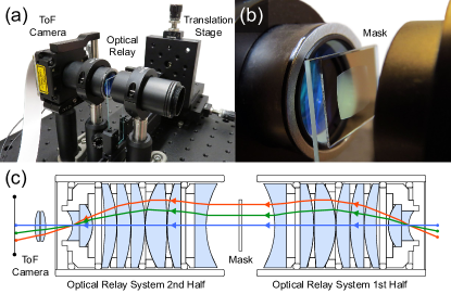
Figure 5: (a) The assembled imaging system. (b) The mask mounted on a precision microscope slide attached to a translation stage. (c) A schematic of the relay lens system.

Mask Fabrication.  We fabricate our custom mask patterns via photolithography. 0.5mm fused silica wafers are used as the substrate, receiving a 200nm of chromium film to occlude light. A layer of 0.6 $\mu$m thick photoresist AZ1505 is then spin-coated on top. We place the wafer under a master mask on a contact aligner (EVG 6200$\infty$) for UV exposure, and develop in AZ726 to form the mask pattern on the photoresist. With an etchant we then remove the chromium from under open areas in the photoresist. See the Supplemental Document for further information on fabrication.

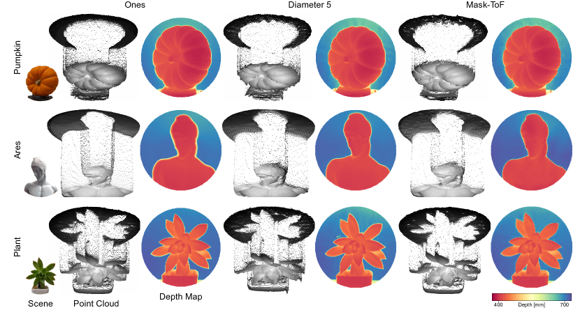
Figure 6: Perspective point cloud visualizations and depth maps of reconstruction results for Mask-ToF and naïve mask designs; object references on the left. Point cloud texture is generated from separate long-exposure amplitude captures.

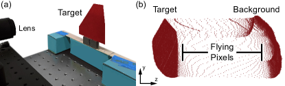
	Ones	Diameter 5	Mask-ToF
Flying Pixel Ratio:	1	0.69	0.48

Figure 7: To quantify flying pixel ratios, we (a) capture 5 flat targets at a known depth and (b) count the number of points between the target and background planes.

Prototype.  We capture measurements with an AMCW ToF camera (Helios Flex, Lucid Vision) operating on an NVIDIA Jetson TX2. We use a custom-designed 1:1 Keplerian telescope as an optical relay system to virtually place the mask on the sensor (see Figure 5). This eliminates the need to remove the sensor cover glass and allows for rapid prototyping, but in a commercial product can be supplanted by a directly integrated mask to maintain device form factor. The mask sits on the intermediate image plane of the telescope attached to a precision microscope slide, which is optically conjugate with the sensor plane. We adjust the position of the mask with an XYZ translation stage (Thorlabs PT3A). For more details, see the Supplemental Document.

Results.  Depth maps were captured via the previously described setup and fed directly into the synthetically trained refinement network $R$, with no network fine-tuning. By counting points as in Figure 7, we see that Mask-ToF cuts flying pixel counts in half when compared to an open aperture. Compared to the near-identical light throughput Diameter 5 mask we reduce FPs by an additional 30.5$\%$. These results are qualitatively confirmed in Figure 6 for objects of varying geometry and reflectance, with additional results in the Supplemental Document and 3D rendering in the accompanying video. Our optimized mask reconstruction visibly and significantly reduces FPs as compared to Diameter 5, while maintaining object shape consistency with the open aperture measurements. Of note is how sharply Mask-ToF reconstructs the tips of the Plant example’s petals, as compared to the noisy reconstruction produced by the Diameter 5 mask. Additionally, Mask-ToF is even able to reduce intra-object FPs such as those inside the Plant’s pot.

7 Conclusion

Mask-ToF is an end-to-end approach to tackle the long-standing problem of flying pixel artifacts in time-of-flight imaging. It learns a per-pixel microlens amplitude mask, that, when combined with a jointly trained refinement network, reduces FPs while preserving light throughput. We validate the method both in simulation and experimentally, manufacturing the learned mask and optically placing it on a camera sensor with a custom-designed optical relay system. The proposed mask and reconstruction method outperform existing hand-engineered masks (and no mask) for real-world scenes. In a mass-market implementation of our method, we envision the amplitude mask to be integrated as part of the sensor assembly, maintaining the camera form-factor while improving FP statistics. Future research directions include learned phase mask patterns and dynamic masks, implemented via a spatial light modulator or similar, which adapt their structure to the observed scene.

Acknowledgements.  This work was supported in part by KAUST baseline funding, Felix Heide’s NSF CAREER Award (2047359) and Sony Faculty Innovation Award, and Ilya Chugunov’s NSF Graduate Research Fellowship.

References

- [1] Narendra Ahuja and A. Lynn Abbott. Active stereo: integrating disparity, vergence, focus, aperture and calibration for surface estimation. IEEE Transactions on Pattern Analysis and Machine Intelligence, 15(10):1007–1029, 1993.
- [2] Phil Ammirato, Patrick Poirson, Eunbyung Park, Jana Košecká, and Alexander C Berg. A dataset for developing and benchmarking active vision. In 2017 IEEE International Conference on Robotics and Automation (ICRA), pages 1378–1385. IEEE, 2017.
- [3] Gonzalo R Arce, David J Brady, Lawrence Carin, Henry Arguello, and David S Kittle. Compressive coded aperture spectral imaging: An introduction. IEEE Signal Processing Magazine, 31(1):105–115, 2013.
- [4] M Salman Asif, Ali Ayremlou, Aswin Sankaranarayanan, Ashok Veeraraghavan, and Richard G Baraniuk. Flatcam: Thin, lensless cameras using coded aperture and computation. IEEE Transactions on Computational Imaging, 3(3):384–397, 2016.
- [5] Seung-Hwan Baek, Diego Gutierrez, and Min H Kim. Birefractive stereo imaging for single-shot depth acquisition. ACM Transactions on Graphics (TOG), 35(6):1–11, 2016.
- [6] Seung-Hwan Baek, Hayato Ikoma, Daniel S Jeon, Yuqi Li, Wolfgang Heidrich, Gordon Wetzstein, and Min H Kim. End-to-end hyperspectral-depth imaging with learned diffractive optics. arXiv preprint arXiv:2009.00463, 2020.
- [7] Clara Callenberg, Felix Heide, Gordon Wetzstein, and Matthias B Hullin. Snapshot difference imaging using correlation time-of-flight sensors. ACM Transactions on Graphics (TOG), 36(6):1–11, 2017.
- [8] Angel X Chang, Thomas Funkhouser, Leonidas Guibas, Pat Hanrahan, Qixing Huang, Zimo Li, Silvio Savarese, Manolis Savva, Shuran Song, Hao Su, et al. Shapenet: An information-rich 3d model repository. arXiv preprint arXiv:1512.03012, 2015.
- [9] Julie Chang and Gordon Wetzstein. Deep optics for monocular depth estimation and 3d object detection. In Proceedings of the IEEE International Conference on Computer Vision, pages 10193–10202, 2019.
- [10] Christopher B Choy, Danfei Xu, JunYoung Gwak, Kevin Chen, and Silvio Savarese. 3d-r2n2: A unified approach for single and multi-view 3d object reconstruction. In European conference on computer vision, pages 628–644. Springer, 2016.
- [11] Shane Colburn, Alan Zhan, and Arka Majumdar. Metasurface optics for full-color computational imaging. Science advances, 4(2):eaar2114, 2018.
- [12] Sergio Cova, Massimo Ghioni, Andrea Lacaita, Carlo Samori, and Franco Zappa. Avalanche photodiodes and quenching circuits for single-photon detection. Applied optics, 35(12):1956–1976, 1996.
- [13] Angela Dai, Angel X Chang, Manolis Savva, Maciej Halber, Thomas Funkhouser, and Matthias Nießner. Scannet: Richly-annotated 3d reconstructions of indoor scenes. In Proceedings of the IEEE Conference on Computer Vision and Pattern Recognition, pages 5828–5839, 2017.
- [14] Angela Dai, Daniel Ritchie, Martin Bokeloh, Scott Reed, Jürgen Sturm, and Matthias Nießner. Scancomplete: Large-scale scene completion and semantic segmentation for 3d scans. In Proceedings of the IEEE Conference on Computer Vision and Pattern Recognition, pages 4578–4587, 2018.
- [15] Jia Deng, Wei Dong, Richard Socher, Li-Jia Li, Kai Li, and Li Fei-Fei. Imagenet: A large-scale hierarchical image database. In 2009 IEEE conference on computer vision and pattern recognition, pages 248–255. Ieee, 2009.
- [16] Dragos Falie and Vasile Buzuloiu. Noise characteristics of 3d time-of-flight cameras. In 2007 International Symposium on Signals, Circuits and Systems, volume 1, pages 1–4. IEEE, 2007.
- [17] Mario Frank, Matthias Plaue, and Fred A Hamprecht. Denoising of continuous-wave time-of-flight depth images using confidence measures. Optical Engineering, 48(7):077003, 2009.
- [18] Ariel Gordon, Hanhan Li, Rico Jonschkowski, and Anelia Angelova. Depth from videos in the wild: Unsupervised monocular depth learning from unknown cameras. In Proceedings of the IEEE International Conference on Computer Vision, pages 8977–8986, 2019.
- [19] Saurabh Gupta, James Davidson, Sergey Levine, Rahul Sukthankar, and Jitendra Malik. Cognitive mapping and planning for visual navigation. In Proceedings of the IEEE Conference on Computer Vision and Pattern Recognition, pages 2616–2625, 2017.
- [20] Dipl-Ing Bianca Hagebeuker and Product Marketing. A 3d time of flight camera for object detection. PMD Technologies GmbH, Siegen, 2007.
- [21] Miles Hansard, Seungkyu Lee, Ouk Choi, and Radu Patrice Horaud. Time-of-flight cameras: principles, methods and applications. Springer Science & Business Media, 2012.
- [22] Felix Heide, Steven Diamond, David B Lindell, and Gordon Wetzstein. Sub-picosecond photon-efficient 3d imaging using single-photon sensors. Scientific reports, 8(1):1–8, 2018.
- [23] Felix Heide, Wolfgang Heidrich, Matthias Hullin, and Gordon Wetzstein. Doppler time-of-flight imaging. ACM Transactions on Graphics (ToG), 34(4):1–11, 2015.
- [24] Heiko Hirschmuller. Accurate and efficient stereo processing by semi-global matching and mutual information. In 2005 IEEE Computer Society Conference on Computer Vision and Pattern Recognition (CVPR’05), volume 2, pages 807–814. IEEE, 2005.
- [25] Katrin Honauer, Ole Johannsen, Daniel Kondermann, and Bastian Goldluecke. A dataset and evaluation methodology for depth estimation on 4d light fields. In Asian Conference on Computer Vision. Springer, 2016.
- [26] Hueihan Jhuang, Juergen Gall, Silvia Zuffi, Cordelia Schmid, and Michael J Black. Towards understanding action recognition. In Proceedings of the IEEE international conference on computer vision, pages 3192–3199, 2013.
- [27] Alex Kendall, Hayk Martirosyan, Saumitro Dasgupta, Peter Henry, Ryan Kennedy, Abraham Bachrach, and Adam Bry. End-to-end learning of geometry and context for deep stereo regression. In Proceedings of the IEEE International Conference on Computer Vision, pages 66–75, 2017.
- [28] Diederik P Kingma and Jimmy Ba. Adam: A method for stochastic optimization. arXiv preprint arXiv:1412.6980, 2014.
- [29] Andreas Kolb, Erhardt Barth, Reinhard Koch, and Rasmus Larsen. Time-of-flight cameras in computer graphics. In Computer Graphics Forum, volume 29, pages 141–159. Wiley Online Library, 2010.
- [30] Johannes Kopf, Michael F Cohen, Dani Lischinski, and Matt Uyttendaele. Joint bilateral upsampling. ACM Transactions on Graphics (ToG), 26(3):96–es, 2007.
- [31] Alex Krizhevsky, Vinod Nair, and Geoffrey Hinton. Cifar-10 (canadian institute for advanced research).
- [32] Alex Krizhevsky, Vinod Nair, and Geoffrey Hinton. Cifar-100 (canadian institute for advanced research).
- [33] Robert Lange. 3d time-of-flight distance measurement with custom solid-state image sensors in cmos/ccd-technology. 2000.
- [34] Robert Lange and Peter Seitz. Solid-state time-of-flight range camera. IEEE Journal of quantum electronics, 37(3):390–397, 2001.
- [35] Felix Järemo Lawin, Per-Erik Forssén, and Hannes Ovrén. Efficient multi-frequency phase unwrapping using kernel density estimation. In European Conference on Computer Vision, pages 170–185. Springer, 2016.
- [36] Nalpantidis Lazaros, Georgios Christou Sirakoulis, and Antonios Gasteratos. Review of stereo vision algorithms: from software to hardware. International Journal of Optomechatronics, 2(4):435–462, 2008.
- [37] Marc Levoy and Pat Hanrahan. Light field rendering. In Proceedings of the 23rd annual conference on Computer graphics and interactive techniques, pages 31–42, 1996.
- [38] David B Lindell, Matthew O’Toole, and Gordon Wetzstein. Single-photon 3d imaging with deep sensor fusion. ACM Transactions on Graphics (TOG), 37(4):1–12, 2018.
- [39] Patrick Llull, Xuejun Liao, Xin Yuan, Jianbo Yang, David Kittle, Lawrence Carin, Guillermo Sapiro, and David J Brady. Coded aperture compressive temporal imaging. Optics express, 21(9):10526–10545, 2013.
- [40] Fangchang Ma, Guilherme Venturelli Cavalheiro, and Sertac Karaman. Self-supervised sparse-to-dense: Self-supervised depth completion from lidar and monocular camera. In 2019 International Conference on Robotics and Automation (ICRA), pages 3288–3295. IEEE, 2019.
- [41] Reza Mahjourian, Martin Wicke, and Anelia Angelova. Unsupervised learning of depth and ego-motion from monocular video using 3d geometric constraints. In Proceedings of the IEEE Conference on Computer Vision and Pattern Recognition, pages 5667–5675, 2018.
- [42] Julio Marco, Quercus Hernandez, Adolfo Munoz, Yue Dong, Adrian Jarabo, Min H Kim, Xin Tong, and Diego Gutierrez. Deeptof: off-the-shelf real-time correction of multipath interference in time-of-flight imaging. ACM Transactions on Graphics (ToG), 36(6):1–12, 2017.
- [43] Kshitij Marwah, Gordon Wetzstein, Yosuke Bando, and Ramesh Raskar. Compressive light field photography using overcomplete dictionaries and optimized projections. ACM Transactions on Graphics (TOG), 32(4):1–12, 2013.
- [44] Enrico Mattei and Alexey Castrodad. Point cloud denoising via moving rpca. In Computer Graphics Forum, volume 36, pages 123–137. Wiley Online Library, 2017.
- [45] Aongus McCarthy, Robert J Collins, Nils J Krichel, Verónica Fernández, Andrew M Wallace, and Gerald S Buller. Long-range time-of-flight scanning sensor based on high-speed time-correlated single-photon counting. Applied optics, 48(32):6241–6251, 2009.
- [46] Andreas Meuleman, Seung-Hwan Baek, Felix Heide, and Min H Kim. Single-shot monocular rgb-d imaging using uneven double refraction. In Proceedings of the IEEE/CVF Conference on Computer Vision and Pattern Recognition, pages 2465–2474, 2020.
- [47] Sofiane Mihoubi, Pierre-Jean Lapray, and Laurent Bigué. Survey of demosaicking methods for polarization filter array images. Sensors, 18(11):3688, 2018.
- [48] Elias Nehme, Daniel Freedman, Racheli Gordon, Boris Ferdman, Lucien E Weiss, Onit Alalouf, Tal Naor, Reut Orange, Tomer Michaeli, and Yoav Shechtman. Deepstorm3d: dense 3d localization microscopy and psf design by deep learning. Nature Methods, 17(7):734–740, 2020.
- [49] Abdul Nurunnabi, Geoff West, and David Belton. Outlier detection and robust normal-curvature estimation in mobile laser scanning 3d point cloud data. Pattern Recognition, 48(4):1404–1419, 2015.
- [50] Gaurav Pandey, James R McBride, and Ryan M Eustice. Ford campus vision and lidar data set. The International Journal of Robotics Research, 30(13):1543–1552, 2011.
- [51] Liliana Lo Presti and Marco La Cascia. 3d skeleton-based human action classification: A survey. Pattern Recognition, 53:130–147, 2016.
- [52] RJ Proctor, GK Skinner, and AP Willmore. The design of optimum coded mask x-ray telescopes. Monthly Notices of the Royal Astronomical Society, 187(3):633–643, 1979.
- [53] Charles R Qi, Hao Su, Kaichun Mo, and Leonidas J Guibas. Pointnet: Deep learning on point sets for 3d classification and segmentation. In Proceedings of the IEEE conference on computer vision and pattern recognition, pages 652–660, 2017.
- [54] Charles Ruizhongtai Qi, Li Yi, Hao Su, and Leonidas J Guibas. Pointnet++: Deep hierarchical feature learning on point sets in a metric space. In Advances in neural information processing systems, pages 5099–5108, 2017.
- [55] Malcolm Reynolds, Jozef Doboš, Leto Peel, Tim Weyrich, and Gabriel J Brostow. Capturing time-of-flight data with confidence. In CVPR 2011, pages 945–952. IEEE, 2011.
- [56] Andreas Rossler, Davide Cozzolino, Luisa Verdoliva, Christian Riess, Justus Thies, and Matthias Nießner. Faceforensics++: Learning to detect manipulated facial images. In Proceedings of the IEEE International Conference on Computer Vision, pages 1–11, 2019.
- [57] Alexander Sabov and Jörg Krüger. Identification and correction of flying pixels in range camera data. In Proceedings of the 24th Spring Conference on Computer Graphics, pages 135–142, 2008.
- [58] Daniel Scharstein and Richard Szeliski. High-accuracy stereo depth maps using structured light. In 2003 IEEE Computer Society Conference on Computer Vision and Pattern Recognition, 2003. Proceedings., volume 1, pages I–I. IEEE, 2003.
- [59] Jamie Shotton, Andrew Fitzgibbon, Mat Cook, Toby Sharp, Mark Finocchio, Richard Moore, Alex Kipman, and Andrew Blake. Real-time human pose recognition in parts from single depth images. In CVPR 2011, pages 1297–1304. Ieee, 2011.
- [60] Shikhar Shrestha, Felix Heide, Wolfgang Heidrich, and Gordon Wetzstein. Computational imaging with multi-camera time-of-flight systems. ACM Transactions on Graphics (ToG), 35(4):1–11, 2016.
- [61] Nathan Silberman, Derek Hoiem, Pushmeet Kohli, and Rob Fergus. Indoor segmentation and support inference from rgbd images. In European conference on computer vision, pages 746–760. Springer, 2012.
- [62] Vincent Sitzmann, Steven Diamond, Yifan Peng, Xiong Dun, Stephen Boyd, Wolfgang Heidrich, Felix Heide, and Gordon Wetzstein. End-to-end optimization of optics and image processing for achromatic extended depth of field and super-resolution imaging. ACM Transactions on Graphics (TOG), 37(4):1–13, 2018.
- [63] Nikolai Smolyanskiy, Alexey Kamenev, and Stan Birchfield. On the importance of stereo for accurate depth estimation: An efficient semi-supervised deep neural network approach. In Proceedings of the IEEE Conference on Computer Vision and Pattern Recognition Workshops, pages 1007–1015, 2018.
- [64] Shuran Song, Samuel P Lichtenberg, and Jianxiong Xiao. Sun rgb-d: A rgb-d scene understanding benchmark suite. In Proceedings of the IEEE conference on computer vision and pattern recognition, pages 567–576, 2015.
- [65] Shuochen Su, Felix Heide, Gordon Wetzstein, and Wolfgang Heidrich. Deep end-to-end time-of-flight imaging. In Proceedings of the IEEE Conference on Computer Vision and Pattern Recognition, pages 6383–6392, 2018.
- [66] Murali Subbarao and Gopal Surya. Depth from defocus: A spatial domain approach. International Journal of Computer Vision, 13(3):271–294, 1994.
- [67] Qilin Sun, Ethan Tseng, Qiang Fu, Wolfgang Heidrich, and Felix Heide. Learning rank-1 diffractive optics for single-shot high dynamic range imaging. In Proceedings of the IEEE/CVF Conference on Computer Vision and Pattern Recognition, pages 1386–1396, 2020.
- [68] Qilin Sun, Jian Zhang, Xiong Dun, Bernard Ghanem, Yifan Peng, and Wolfgang Heidrich. End-to-end learned, optically coded super-resolution spad camera. ACM Transactions on Graphics (TOG), 39(2):1–14, 2020.
- [69] Ethan Tseng, Felix Yu, Yuting Yang, Fahim Mannan, Karl ST Arnaud, Derek Nowrouzezahrai, Jean-François Lalonde, and Felix Heide. Hyperparameter optimization in black-box image processing using differentiable proxies. ACM Trans. Graph., 38(4):27–1, 2019.
- [70] Shubham Tulsiani, Alexei A Efros, and Jitendra Malik. Multi-view consistency as supervisory signal for learning shape and pose prediction. In Proceedings of the IEEE conference on computer vision and pattern recognition, pages 2897–2905, 2018.
- [71] Xiang-Gen Xia and Genyuan Wang. Phase unwrapping and a robust chinese remainder theorem. IEEE Signal Processing Letters, 14(4):247–250, 2007.
- [72] Lei Xiao, Felix Heide, Matthew O’Toole, Andreas Kolb, Matthias B Hullin, Kyros Kutulakos, and Wolfgang Heidrich. Defocus deblurring and superresolution for time-of-flight depth cameras. In Proceedings of the IEEE Conference on Computer Vision and Pattern Recognition, pages 2376–2384, 2015.
- [73] Haofei Xu and Juyong Zhang. Aanet: Adaptive aggregation network for efficient stereo matching. In Proceedings of the IEEE/CVF Conference on Computer Vision and Pattern Recognition, pages 1959–1968, 2020.
- [74] Shi Yan, Chenglei Wu, Lizhen Wang, Feng Xu, Liang An, Kaiwen Guo, and Yebin Liu. Ddrnet: Depth map denoising and refinement for consumer depth cameras using cascaded cnns. In Proceedings of the European conference on computer vision (ECCV), pages 151–167, 2018.
- [75] Xinchen Yan, Jimei Yang, Ersin Yumer, Yijie Guo, and Honglak Lee. Perspective transformer nets: Learning single-view 3d object reconstruction without 3d supervision. In Advances in neural information processing systems, pages 1696–1704, 2016.
- [76] Matthew D Zeiler and Rob Fergus. Visualizing and understanding convolutional networks. In European conference on computer vision, pages 818–833. Springer, 2014.