On AO*, Proof Number Search and Minimax Search

Abstract

We discuss the interconnections between AO*, adversarial game-searching algorithms, e.g., proof number search and minimax search. The former was developed in the context of a general AND/OR graph model, while the latter were mostly presented in game-trees which are sometimes modeled using AND/OR trees. It is thus worth investigating to what extent these algorithms are related and how they are connected. In this paper, we explicate the interconnections between these search paradigms. We argue that generalized proof number search might be regarded as a more informed replacement of AO* for solving arbitrary AND/OR graphs, and the minimax principle might also extended to use dual heuristics.

1 Introduction

The advancements of heuristic search algorithms have seen separate developments in the AI planning Bonet and Geffner (2001) and in two-player games communities, where the search spaces are respectively modeled as an OR graph and AND/OR graph Pearl (1984). The core algorithm for searching OR graph is A* Hart et al. (1968), whose aspiration is a shortest path-finding. Since its invention, many subsequent work have been carried out to further improve various aspects of the algorithm, e.g., IDA* Korf (1985) for reduced space usage and LRTA* Korf (1990) for real-time behavior. While early work showed that generalizing A* to AND/OR graphs results AO* Chang and Slagle (1971); Nilsson (1980), by comparison, much less subsequent effort have been devoted to this line of research.

For adversarial game-searching, earliest work dates back to Samuel’s studies in checkers Samuel (1959), where a minimax search is used with Alpha-Beta pruning Knuth and Moore (1975). This kind of minimax search continued to improve as computers become faster and more general or game-specific searching techniques were introduced, culminating to the successes of champion playing strength in games such as chess Campbell et al. (2002). Instead of just game-playing, the other research direction aims at game-solving, whose goal is to use limited resource to find the game-theoretic result of a game. Alpha-Beta Knuth and Moore (1975) style depth-first search can also be used for this goal, but its unsatisfying practical performance pushed researchers to devise search algorithms specialized for solving. Proof number search (PNS) Allis (1994) was developed of such. Together with other game-specific advancements, PNS and its variant Nagai (2002) have been used for successfully solving a number of games, e.g., Gomoku Allis (1994), checkers Schaeffer et al. (2007).

However, algorithms for games were mostly developed without much referring to advancements in the heuristic search planning community, and vice versa. There have been little discussion on how algorithms from these two communities are related. In this paper, we aim to bridge this conceptual gap by presenting a through investigation on the relationship between AO*, PNS and Minimax search paradigms.

2 Preliminaries

2.1 AND/OR Graphs

AND/OR graph is a form of directed graph that can be used to represent problem solving using problem reduction. Comparing to normal graphs, the additional property for an AND/OR graph is that any edge coming out of a node is labeled either as an OR or AND edge. A node contains only OR outgoing edges is called an OR node. Conversely, a node emitting only AND edges is called an AND node. Any node emanating both AND and OR edges is called mixed node. To distinguish, in graphic notation, all AND edges from the same node are often grouped using an arc. It is also easy to see that any mixed node can be replaced with two pure AND and OR nodes Pearl (1984). Due to this reason, in this text, we shall assume an AND/OR graph contains only pure AND and OR nodes, such that explicitly distinguishing edge types becomes unnecessary. One can note a graph of such using a tuple $G=<$$V_{o},V_{a},E$$>$, where $V_{o}$ and $V_{a}$ are respectively the set of OR and AND nodes, and $E$ represents the set of directed edges.

The AND nodes can be interpreted in different ways. In the deterministic view, an AND node represents that solving this node would require to sequentially solving all its child nodes. Figure 1 shows an example, where the graph can be interpreted as that “to solve problem $A$, either $B$ and $C$ must be solved, to solve $B$, both $D$ and $E$ have to be solved, while for solving $C$, only $E$ or $F$ needs to be solved”. Clearly, in this context, the graph must be directed and acyclic as any violation would represents a cyclic reasoning, rendering the graph itself paradoxical.

Figure 1: Directed acyclic AND/OR graph represents problem-reduction reasoning.

Another interpretation views an AND node as a probabilistic node, such that AND/OR graphs can be used as a model of Markov decision processes (MDPs) Howard (1960), where cycles are totally legitimate. However, solving AND/OR graphs of such inevitably invokes dynamic programming Hansen and Zilberstein (2001). In this paper, we exclusively focus on directed AND/OR graphs without cycles. Another interpretation views an AND node as a probabilistic or change node. In this view, an AND/OR graph can be used as a graph model for Markov decision processes (MDPs) Howard (1960). Each OR node in MDP is regarded as a state, where an agent can take actions, but taking an action would possibly result different next states, drawn from a fixed probability distribution. An MDP is solved when the optimal value of each state is known, thus at any state, agent can always choose to take the action that would result the maximum expected next state value, fulfilling its objective. In this MDP case, loop does not affect its solvability. Figure 2 shows an example. However, solving AND/OR graphs of such inevitably invokes dynamic programming Hansen and Zilberstein (2001). In this paper, we mainly focus on directed AND/OR graphs without cycles.

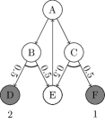
Figure 2: Directed AND/OR graph represents Markov decision process. $D$ and $F$ are terminal nodes whose optimal values are given as $2$ and $1$. There are two actions at $A$. If taking the action to $B$, $value(A)=0.5\cdot 2+0.5\cdot value(A)\Rightarrow value(A)=2$. If taking action to $C$, then $value(A)=0.5\cdot 1+0.5\cdot value(A)\Rightarrow value(A)=1$. Thus, to maximize the value at $A$, action to $B$ is optimal.

In Figure 1, we see that if we assume $A$ is solvable, in the best case, only one sub-problem $E$ is required to be solvable to validate our assumption. Conversely, knowing only $E$ and $F$ both are unsolvable is enough to say that $A$ is unsolvable. In other words, the minimum number of leaf nodes to examine for proving $A$ is 1, and $2$ for disproving. The sub-graph that used to claim either $A$ is solvable or unsolvable is called solution-graph. For Figure 1, a solvable solution-graph can be $\{A\to C\to E\}$, assuming $E$ is solvable; an unsolvable solution-graph can be $\{A\to C\to E,C\to F\}$ assuming both $E$ and $F$ are unsolvable.

2.2 AO* for Acyclic AND/OR Graphs

In practice, the complete AND/OR graph is usually too large to be explicitly represented prior solving. Heuristic search algorithms therefore aspire to generate only a small portion of the whole graph to find the desired solution. The complete and hidden graph is therefore called implicit graph $G$, while the partial graph search is operating on is called explicit graph $G^{\prime}$.

Frontier nodes in implicit $G^{\prime}$ having no successors are called leaf nodes; a leaf node whose value is immediately-known is called terminal whose status can be solvable or unsolvable — they can respectively be assigned with values $0$ and $\infty$ in the context of cost minimization. The process of generating successors for a non-terminal leaf node is called expansion. Starting from a single node, heuristic search paradigm AO* Nilsson (1980) enlarges $G^{\prime}$ gradually by node expansion until the start node is SOLVED, i.e., either being proved as solvable or unsolvable.

We detail AO* in Algorithm 1. It can be viewed as a repetition of two major operations: a top-down graph growing procedure, and a bottom-up cost revision procedure. The top-down operation traces a most promising partial solution graph from marked edges, while the bottom-up revision modifies the necessary edge marking due to new information provided by node expansion, guaranteeing that for the next iteration most promising partial solution graph can still be synthesized by tracing marked edges. AO* returns an “optimal” additive-cost solution graph given the heuristic function $h$ is admissible Martelli and Montanari (1973).

1 Let the explicit graph be $G^{\prime}=\{s\}$, initialize cost $f(s)=h(s)$

2 while  $label(s)\neq\mathit{SOLVED}$  do

3       Compute a partial solution graph $G_{0}$ following marked edges in $G^{\prime}$

4       Select any non-terminal leaf node $n$ in $G_{0}$

5       Expand $n$, add each of its successor $n_{j}$ to $G^{\prime}$ if $n_{j}\not\in G^{\prime}$

6       for each new successor $n_{j}$ of $n$ do

7             $label(n_{j})\leftarrow\mathit{SOLVED}$ if $n_{j}$ is terminal

8             Otherwise, $f(n_{j})\leftarrow h(n_{j})$

9            

10       end for

11      Let $S\leftarrow\{n\}$

12       while $S\neq\emptyset$ do

13             Remove $m$ from $S$ such that $m$ has no descendants in $G^{\prime}$ occurring in $S$

14              if $m$ is OR node then

15                   $x\leftarrow\min\{c(m,m_{i})+f(m_{i})|i=1,\ldots,k\}$

16                   Mark the edge where the minimum is achieved

17                   Set $label(m)\leftarrow\mathit{SOLVED}$ if the minimum successor is SOLVED;

18            else

19                   $x\leftarrow\sum_{i=1}^{k}c(m,m_{i})+f(m_{i})$

20                   Mark each edge from $m$ to $m_{i}$

21                   Set $label(m)\leftarrow\mathit{SOLVED}$ if all successors are SOLVED

22             end if

23            if $q(m)\neq x$ or $label(m)=\mathit{SOLVED}$ then

24                   $q(m)\leftarrow x$

25                   Add those parents of $m$ to $S$ such that $m$ is one of their successors through a marked edge

26             end if

27            

28       end while

29      

30 end while

31

Algorithm 1 AO* algorithm

2.3 Proof Number Search for Game-Trees

AND/OR trees can be used to model search space of adversarial games Nilsson (1980), where the additional regularity is that OR and AND appear alternately in layers. If we use $\phi(x)$ and $\delta(x)$ to respectively denote the minimum effort to use in order to prove that a state $x$ is winning and losing. A node is said to be a winning (i.e., solvable) state if the player to play at that node wins, respectively for losing (i.e., unsolvable). Clearly, $\phi(x)$ is dependent on $delta$ values of its children $succ(x)$, and $\delta(x)$ can be derived from the $\phi$ values of $succ(x)$. Proof number search Allis (1994) uses the following equation to compute $\phi$ and $\delta$ for node $x$:

$$\small\begin{array}[]{l}\phi(x)=\begin{cases}1\qquad\mbox{$x$ is non-terminal leaf node}\\ 0\qquad\mbox{$x$ is terminal winning state}\\ \infty\qquad\mbox{$x$ is terminal losing state}\\ \min\limits_{x_{j}\in succ(x)}\delta(x_{j})\\ \end{cases}\\ \\ \delta(x)=\begin{cases}1\qquad\qquad\mbox{$x$ is non-terminal leaf node}\\ \infty\qquad\mbox{$x$ is terminal winning state}\\ 0\qquad\mbox{$x$ is terminal losing state}\\ \sum_{x_{j}\in succ(x)}\phi(x_{j})\\ \end{cases}\end{array}$$ (1)

Since any non-terminal leaf is given a value of 1, by Eq. (5), we see $\phi(x)$ and $\delta(x)$ can be interpreted as the minimum number of non-terminal leaf nodes in order to prove or disprove $x$. Equipped with Eq. (5), PNS conducts a best-first search repeatedly doing the following steps:

1. Selection. Starting from the root, at each node $x$: select a child node with the minimum $\delta$ value, stop until $x$ is a leaf node.

2. Evaluation and Expansion. Check if the leaf is a terminal or not. If not, the leaf node is expanded and all its newly children are assigned with $(\phi,\delta)\leftarrow(1,1)$.

3. Backup. Updated proof and disproof numbers for the selected leaf node is back-propagated up to the tree according to Eq. (5).

In practice, the df-pn Nagai (2002) variant can be used to reduce PNS’s space usage. Given sufficient memory and computation time, it has been shown that df-pn are also complete in directed acyclic AND/OR graphs Kishimoto and Müller (2008).

3 Relation of AO*, PNS and Minimax

In this section, we examine the connections between AO* and PNS. We start by an abstract and general best-first search depicted in Pearl (1984), then show how AO* and PNS can be arrived by grounding different specific functions, and how one algorithm can be another by restricting certain definitions on which the search operates.

3.1 General Best First Search

A General Best-first Search (GBFS) has summarized in  Pearl (1984) for solving directed and acyclic AND/OR graphs. We reiterate it as in Algorithm 2. Notably, GBFS includes A*, AO* all as its special variant. In Algorithm 2, three abstract functions $f_{1}$, $f_{2}$ and $h$ are respectively used for selecting the partial solution graph (or solution-base as in Pearl (1984)) $G_{0}$ in $G^{\prime}$, choosing a leaf node $n$ from $G_{0}$ for expansion, and evaluating $n$. The implementation of $f_{1}$ and $f_{2}$ depends on how a candidate solution is evaluated and what cost scheme is used to define such evaluation.

Input: Start node $s$, selection function $f_{1},f_{2}$, rules for generating successor nodes, evaluation function $h$, cost scheme $\Psi$

Output: Solution graph $G_{0}^{*}$

1 Function GBFS($s$, $f_{1}$, $f_{2}$):

2       Let the explicit graph be $G^{\prime}=\{s\}$

3       while  $true$  do

4             $G_{0}\leftarrow f_{1}(G^{\prime})$ // $G_{0}$ is solution-base

5             if  $G_{0}$ is solution graph then

6                   $G_{0}^{*}\leftarrow G_{0}$, then exit;

7             end if

8            $t\leftarrow f_{2}(G_{0})$ // $t$ is selected frontier node

9             Generate all successors of $t$, append to $G^{\prime}$

10             for $t^{\prime}\in successor(t)$ do

11                   Evaluate $t^{\prime}$ by $h$

12                   UpdateAncestors$(t^{\prime},\Psi,G^{\prime})$

13                  

14             end for

15            

16       end while

17      return $G_{0}^{*}$

18      

19

20 Function UpdateAncestors($t^{\prime}$, $\Psi$, $G^{\prime}$):

21       Update ancestor nodes of $t^{\prime}$ in $G^{\prime}$ according to the definition of $\Psi$

22      

23

Algorithm 2 General Best-First Search

3.2 GBFS and AO*

A recursive cost scheme can be used to facilitate the implementations of $f_{1}$, $f_{2}$. As in Pearl (1984), we say a cost scheme $\Psi$ is recursive if for any node $n$ in $G$, the optimal cost rooted at $n$, namely $h^{*}(n)$, is defined recursively:

$$h^{*}(n)=\begin{cases}\Psi_{n^{\prime}}\big{(}c(n,n^{\prime})+h^{*}(n^{\prime})\big{)}\quad\mbox{ $n$ is AND node}\\ \min_{n^{\prime}}\big{(}c(n,n^{\prime})+h^{*}(n^{\prime})\big{)}\quad\mbox{ $n$ is OR node}\\ 0\quad\mbox{$n$ is solvable terminal}\\ \infty\quad\mbox{$n$ is unsolvable terminal}\\ \end{cases}$$ (2)

Here, $c(n,n^{\prime})\geq 0$ is the edge cost between $n$ and its successor $n^{\prime}$.

Similarly, for arbitrary $n$ in the explicit search graph $G^{\prime}$, given a heuristic function $h$, an estimation for the cost rooted at $n$, denoted by $f(n)$, is defined as follows:

$$f(n)=\begin{cases}\Psi_{n^{\prime}}\big{(}c(n,n^{\prime})+f(n^{\prime})\big{)}\quad\mbox{$n$ is non-leaf AND node}\\ \min\limits_{n^{\prime}}\big{(}c(n,n^{\prime})+f(n^{\prime})\big{)}\quad\mbox{$n$ is non-leaf OR node}\\ 0\quad\mbox{if $n$ is solvable terminal}\\ \infty\quad\mbox{if $n$ is unsolvable terminal}\\ h(n)\quad\mbox{$n$ non-terminal leaf node}\\ \end{cases}$$ (3)

By this recursive definition, $f_{1}$ can select a partial solution-graph $G_{0}$ in this way: starting from $s$, at each OR node, it only needs to select the minimum child node; at each AND node, all successors must be selected. Many potential functions can be used for $\Psi$, such as $\sum$, $\max$ and expected-sum. The recursively definition makes the UpdateAncestors procedure in Algorithm 2 straightforward — after each expansion, all ancestral nodes in $G^{\prime}$ just need to be updated in bottom-up manner by Equation (2). The next question to answer is how $f_{2}$ selects frontier nodes for expansion (except in some special cases only one frontier exists in the $G_{0}$, e.g., for pure OR graphs). If we choose $f_{2}$ to be a uniform random function, and let $\Psi=\sum$, it is clear that a GBFS of such becomes equivalent to AO*: the edge marking and revision step in AO* are just a delicate way to implement $f_{1}$.

One property of AO* is that the selection of leaf node from $G_{0}$ for expansion is arbitrary. Its potential drawback is illustrated in Figure 3.

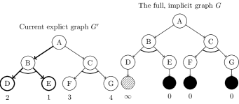
Figure 3: For AO*, if $D$ is expanded first, $E$ will never be expanded; however, if $E$ is chosen first, both $D$ and $E$ will be expanded before the search switches to correct branch $C$. We assume all edges in the graph have a cost of $4$, therefore the estimation provided by $h$ in $G^{\prime}$ is admissible.

3.3 From GBFS and AO* to PNS*

For proof number search, the mechanism for making decisions at AND nodes is essentially symmetric to how AO* implements function $f_{1}$ at OR nodes. So, in general, if we equip a pair of functions to AO* based on two heuristics — one for selecting in OR nodes while the other for AND nodes — a top down selection scheme, which eventually selects a single leaf node for expansion, exists. To indicate the resulting algorithm’s resemblance to PNS, we shall call it PNS*. Denote $\{p(n),d(n)\}$ as the estimated cost rooted at node $n$ in $G^{\prime}$, we have the following recursive relations:

$$\begin{array}[]{l}p(n)=\begin{cases}h(n)\qquad\mbox{$n$ is non-terminal leaf node}\\ \min\limits_{n_{j}\in succ(n)}\big{(}c(n,n_{j})+p(n_{j})\big{)}~{}\mbox{$n$ is OR node}\\ \mathop{\Psi}\limits_{n_{j}\in succ(n)}\big{(}c(n,n_{j})+p(n_{j})\big{)}~{}\mbox{$n$ is AND node}\\ 0~{}\mbox{$n$ is solvable terminal}\\ \infty~{}\mbox{$n$ is unsolvable terminal}\\ \end{cases}\\ \\ d(n)=\begin{cases}\bar{h}(n)\qquad\qquad\mbox{$n$ is non-terminal leaf node}\\ \min\limits_{n_{j}\in succ(n)}\big{(}c(n,n_{j})+d(n_{j})\big{)}~{}\mbox{$n$ is AND node}\\ \mathop{\Psi}\limits_{n_{j}\in succ(n)}\big{(}c(n,n_{j})+d(n_{j})\big{)}~{}\mbox{$n$ is OR node}\\ 0~{}\mbox{$n$ is unsolvable terminal}\\ \infty~{}\mbox{$n$ is solvable terminal}\\ \end{cases}\end{array}$$ (4)

The optimal cost functions $h^{*}(n)$ and $\bar{h}^{*}(n)$ can be defined on the implicit graph $G$ in the same fashion where all leaf nodes are terminal. With Eq. (4), PNS* selects a frontier node to expand with a top-down procedure: at each OR node, it selects a successor $n_{j}$ with the minimum $p(n_{j})$ value, otherwise $n_{i}$ with the minimum $d(n_{i})$ value. Figure 4 demonstrates the merit of PNS* using two heuristics.

Recall the regularity in the AND/OR graph of a two-player alternate-turn game is that AND and OR nodes appear alternately in layers; thus, we might define $p$ and $d$ in an intermingle manner just as Eq. (5). Then, the $h(n)$ and $\bar{h}(n)$ can be interpreted as the difficulty of proving $n$ is winning or losing (with respect to the player to play at $n$), respectively. If using $\sum$ for $\Psi$, letting $h=\bar{h}=1$ (i.e., be a constant function) and all edge cost $c(n,n_{j})=0$, Eq. (4) becomes exactly Eq. (5), and PNS* exactly becomes PNS, except that PNS was originally defined on trees.

To clearly show the relation between AO* and PNS*, we define the concept of dual graph in below.

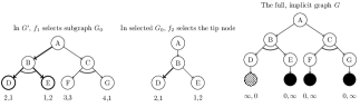
Figure 4: The same as Figure 3, each edge has a cost of 4. The difference is that now each leaf node has a pair of heuristic estimations, respectively representing the estimated cost for being solvable and unsolvable. All leaf nodes are with admissible estimations from both $h_{1}$ and $h_{2}$. Here $h_{2}$ successfully discriminates that $D$ is superior to $E$ because $h_{2}(D)<h_{2}(E)$. Indeed, as long as $h_{2}(D)\in[0,4]\wedge h_{2}(E)\in[0,\infty]$, $h_{2}$ will be admissible, hinting that the chance that an arbitrary admissible $h_{2}$ can successfully choose $D$ is high. Respecting PNS, we call algorithm AO* employing a pair of admissible heuristics PNS*.

Definition 1.

Suppose arbitrary AND/OR graph is noted as $G=\{V_{a},V_{o},E\}$, where $V_{a}$ and $V_{o}$ are respectively the set of AND and OR nodes, $E$ is the set of edges. The dual of $G$, denoted as $\bar{G}$ is defined as $\{\bar{V_{a}},\bar{V_{o}},E\}$ where $\bar{V_{a}}=V_{o},\bar{V_{o}}=V_{a}$. That is, $\bar{G}$ is obtained by reversing all AND nodes from $G$ into OR nodes in $\bar{G}$, all OR nodes from $G$ into AND nodes in $\bar{G}$, all edges remain unchanged.

Then, we have the following observation.

Proposition 1.

For arbitrary node $n$ in AND/OR graph $G$, $p(n)$ and $d(n)$ are recursive cost schemes respectively defined on $G$ and $\bar{G}$. Let $G_{0}\leftarrow f_{1}(G)$, $\bar{G_{0}}\leftarrow f_{1}(\bar{G})$, then, at each iteration, the leaf node selected by PNS* for expansion is the unique intersecting leaf node between $G_{0}$ and $\bar{G_{0}}$.

Thus, we can derive the following result.

Proposition 2.

Given the same tie-breaking and $h$ from AO* is identical to the one in PNS*, then for the same explicit graph $G^{\prime}$, the leaf node selected by PNS* must also be a leaf node in the solution base $G_{0}$ selected by AO*.

Now it is clear that both AO* and PNS* can be viewed as a specific variant of the other.

Proposition 3.

PNS* can be viewed a version of AO*, where $f_{2}(G_{0})$ is implemented by selecting the unique leaf node of the intersection between $f_{1}(G^{\prime})$ and $f_{1}(\bar{G^{\prime}})$. Conversely, AO* can also be viewed as a less informed variant of PNS* by treating all edge cost as $0$ in $\bar{G^{\prime}}$ and $\bar{h}=0$ when applying $f_{1}(\bar{G^{\prime}})$.

In heuristic search, e.g., A*, it is known that algorithm $A$ would dominate algorithm $B$ if the heuristic function $h_{A}$ is more informed than $h_{B}$ Pearl (1984). After seeing that PNS* can be a more informed version of AO*, we conjecture that PNS* might be regarded a general replacement of AO*.

Conjecture 1.

PNS* dominates AO*, given that AO* uses heuristic function $h$, and PNS* uses heuristics $h$ and $\hat{h}$; they use the same recursive cost scheme $\Psi$; both $h$ and $\bar{h}$ are admissible and consistent.

3.4 PNS* and Minimax

Further, in Eq. (4), if we let $\Psi=\max$, restrict edge cost to $0$, and force $h(n)+\bar{h}(n)=C$ for any non-terminal leaf, where $C$ is a constant, then the resulting formula becomes the minimax principle in adversarial games, where the negated cost function $-h$ becomes exactly the evaluation function used in minimax game-searching. In such case, the PNS* algorithm becomes best-first minimax, whose merit has been investigated in Korf and Chickering (1996).

It is known that minimax search may behave poorly in some cases where the evaluation function is not sufficiently reliable Nau (1983). Instead of restricting $h(\cdot)+\bar{h}(\cdot)=C$, it is question how they would behave when two unrelated heuristic evaluation functions are used. The algorithm would still be compatible with Alpha-Beta style pruning, but to our best knowledge, no studies have been carried out along this line of research.

To illustrate how to arrive inimax from PNS*, assuming edge cost are 0, use $\phi(x)$ and $\delta(x)$ to respectively denote the minimum effort to use in order to prove that a state $x$ is winning and losing.

$$\small\begin{array}[]{l}\phi(x)=\begin{cases}h(x)\qquad\mbox{$x$ is non-terminal leaf node}\\ 0\qquad\mbox{$x$ is terminal winning state}\\ \infty\qquad\mbox{$x$ is terminal losing state}\\ \min\limits_{x_{j}\in succ(x)}\delta(x_{j})\\ \end{cases}\\ \\ \delta(x)=\begin{cases}\bar{h}(x)\qquad\qquad\mbox{$x$ is non-terminal leaf node}\\ \infty\qquad\mbox{$x$ is terminal winning state}\\ 0\qquad\mbox{$x$ is terminal losing state}\\ \mathop{\Psi}\limits_{x_{j}\in succ(x)}\phi(x_{j})\\ \end{cases}\end{array}$$ (5)

In Eq. (5), $\Psi$ is a function which can either be max or sum. If $\Psi=\mathit{max}$ and $\infty>h(x)=-h^{\prime}(x)>0$, then Eq. (5) becomes minimax, except that in minimax the leaf evaluation is usually regarded as a score of merit rather than a cost. See Figure 5 for a demonstration. If $\Psi=\mathit{sum}$ and $h(x)=h^{\prime}(x)=1$, Eq. (5) becomes basis for proof number search.

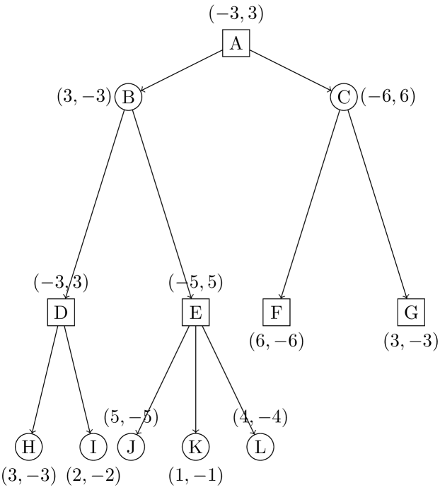
(a) Each node has a pair of evaluations $(\phi,\delta)$, computed bottom up as in Eq. 5 with $\Psi=\mathit{max}$.

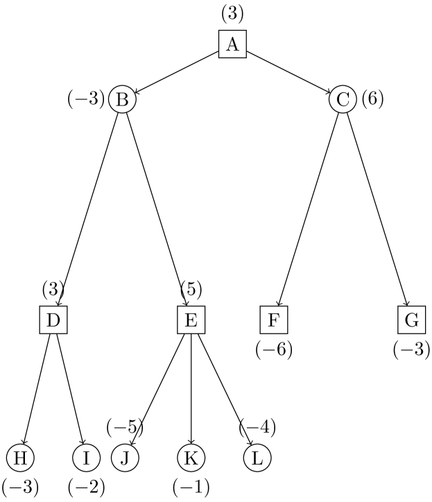
(b) An equivalent $\delta$ only tree that uses conventional negamax for bottom-up computation.

Figure 5: Minimax example in a game-tree. If forcing $\phi+\delta=0$, and use $\Psi=\max$, then we derive Negamax from PNS.

In either case, a game-tree can be instantly solved when all leaf nodes are terminal. Figure 6 shows an example. The root is with $(0,\infty)$, indicating root is a winning state. There are in total two sub-trees, $\{A\to B\to D\to I,B\to E\to L\}$ and $\{A\to C\to F,C\to G\}$. Each of these two sub-trees can be a solution-tree to the game-tree depicted in Figure 6; computing by minimax and mini-sum gives the same result.

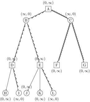
Figure 6: Two solution-trees exist for this game-tree. The “saw” decorated solution-tree contains 6 nodes. The “bumps” decorated solution-tree has 4 nodes.

4 Related Discussions

There have been few discussions on the relations between AO*, PNS and other minimax game-searching algorithms. Allis (1994) detailed the empirical advantages of PNS over other minimax algorithms for solving various games. Discussion on AO* and PNS most related to ours were presented by Nagai (2002), where a depth-first reformulated PNS (df-pn) variant was proposed, and a generalized version df-pn⁺, which includes edge costs, was further described. Nagai (2002) mentioned AO* might be regarded as df-pn⁺ with only proof numbers, but little discussion were provided. In both Nagai (2002) and Allis (1994), PNS was regarded as an algorithm seemingly unrelated to more traditional minimax search. Nilsson (1980) in-depth discussed various aspects of AO*, including other possible ways to select a leaf in the partial solution graph for expansion, such as selecting the one with highest $h$ value, but failed short from proposing a second heuristic function to enhance AO*. Our exposition of the general best first search is adapted from Pearl (1984), who detailed an analysis of single- and two-agent search heuristic search algorithms to that date, before the invention of proof number search.

5 Game-Playing Algorithms

A large amount effort have been devoted to just heuristically playing well: these algorithms are usually developed based on the minimax formulation and they differ majorly in how the heuristic evaluation is constructed and how the search is conducted (i.e., depth-first or best-first). Using a single heuristic evaluation, Alpha-Beta Knuth and Moore (1975) pruning tries to approximate the optimal move by performing a fixed-depth depth-first search. SSS* Stockman (1979) achieves more aggressive pruning using best-first search. For Alpha-Beta, the continual development of methods for constructing reliable evaluations have resulted computer programs defeating top human professionals games like checkers Schaeffer et al. (1992), chess Campbell et al. (2002) and Othello Buro (1998), but not for games where a reliable heuristic evaluation is difficult to construct and the branching factor is large, such as Go Müller (2002) and Hex Van Rijswijck (2002). Monte Carlo tree search (MCTS) Coulom (2006); Kocsis and Szepesvári (2006) was then developed, whose major superiority is its flexibility of integrating learned heuristic evaluations Gelly and Silver (2007). The continual effort towards adding more accurate prior knowledge to MCTS leads to the development of AlphaGo Silver et al. (2016) for playing Go, and AlphaZero Silver et al. (2018), producing strong players in Go, chess and Shogi, after separate training the evaluation functions for each of them.

6 Conclusions

We have provided a comprehensive account on the relations between AO* for general AND/OR graphs and adversarial search for games. Our discussion would help clarify some elusive conceptions concerning heuristic search algorithms for AND/OR graphs and games. There have been application of proof number search to non-game domains Kishimoto et al. (2019). We hope our discussion would inspire more researchers to adopt the advancements from game-searching algorithms to real-world problems with AND/OR structures.

References

- Allis [1994] LV Allis. Searching for solutions in games and artificial intelligence. PhD thesis, Universiteit Maastricht, 1994.
- Bonet and Geffner [2001] Blai Bonet and Héctor Geffner. Planning as heuristic search. Artificial Intelligence, 129(1-2):5–33, 2001.
- Buro [1998] Michael Buro. From simple features to sophisticated evaluation functions. In International Conference on Computers and Games, pages 126–145. Springer, 1998.
- Campbell et al. [2002] Murray Campbell, A Joseph Hoane, and Feng-hsiung Hsu. Deep Blue. Artificial intelligence, 134(1-2):57–83, 2002.
- Chang and Slagle [1971] Chin-Liang Chang and James R. Slagle. An admissible and optimal algorithm for searching AND/OR graphs. Artificial Intelligence, 2(2):117–128, 1971.
- Coulom [2006] Rémi Coulom. Efficient selectivity and backup operators in Monte-Carlo tree search. In International Conference on Computers and Games, pages 72–83. Springer, 2006.
- Gelly and Silver [2007] Sylvain Gelly and David Silver. Combining online and offline knowledge in UCT. In Proceedings of the 24th international conference on Machine learning, pages 273–280. ACM, 2007.
- Hansen and Zilberstein [2001] Eric A Hansen and Shlomo Zilberstein. LAO*: A heuristic search algorithm that finds solutions with loops. Artificial Intelligence, 129(1-2):35–62, 2001.
- Hart et al. [1968] Peter E Hart, Nils J Nilsson, and Bertram Raphael. A formal basis for the heuristic determination of minimum cost paths. IEEE transactions on Systems Science and Cybernetics, 4(2):100–107, 1968.
- Howard [1960] Ronald A Howard. Dynamic programming and Markov processes. 1960.
- Kishimoto and Müller [2008] Akihiro Kishimoto and Martin Müller. About the completeness of depth-first proof-number search. In International Conference on Computers and Games, pages 146–156. Springer, 2008.
- Kishimoto et al. [2019] Akihiro Kishimoto, Beat Buesser, Bei Chen, and Adi Botea. Depth-first proof-number search with heuristic edge cost and application to chemical synthesis planning. In Advances in Neural Information Processing Systems, pages 7224–7234, 2019.
- Knuth and Moore [1975] Donald E Knuth and Ronald W Moore. An analysis of alpha-beta pruning. Artificial intelligence, 6(4):293–326, 1975.
- Kocsis and Szepesvári [2006] Levente Kocsis and Csaba Szepesvári. Bandit based Monte-Carlo planning. In European conference on machine learning, pages 282–293. Springer, 2006.
- Korf and Chickering [1996] Richard E Korf and David Maxwell Chickering. Best-first minimax search. Artificial intelligence, 84(1-2):299–337, 1996.
- Korf [1985] Richard E Korf. Depth-first iterative-deepening: An optimal admissible tree search. Artificial intelligence, 27(1):97–109, 1985.
- Korf [1990] Richard E Korf. Real-time heuristic search. Artificial intelligence, 42(2-3):189–211, 1990.
- Martelli and Montanari [1973] Alberto Martelli and Ugo Montanari. Additive AND/OR graphs. In IJCAI, volume 73, pages 1–11, 1973.
- Müller [2002] Martin Müller. Computer Go. Artificial Intelligence, 134(1-2):145–179, 2002.
- Nagai [2002] Ayumu Nagai. Df-pn algorithm for searching AND/OR trees and its applications. PhD thesis, PhD thesis, Department of Information Science, University of Tokyo, 2002.
- Nau [1983] Dana S Nau. Pathology on game trees revisited, and an alternative to minimaxing. Artificial intelligence, 21(1-2):221–244, 1983.
- Nilsson [1980] Nils J Nilsson. Principles of artificial intelligence. Morgan Kaufmann, 1980.
- Pearl [1984] Judea Pearl. Heuristics: intelligent search strategies for computer problem solving. 1984.
- Samuel [1959] A. L. Samuel. Some studies in machine learning using the game of checkers. IBM J. Res. Dev., 3(3):210–229, July 1959.
- Schaeffer et al. [1992] Jonathan Schaeffer, Joseph Culberson, Norman Treloar, Brent Knight, Paul Lu, and Duane Szafron. A world championship caliber checkers program. Artificial Intelligence, 53(2-3):273–289, 1992.
- Schaeffer et al. [2007] Jonathan Schaeffer, Neil Burch, Yngvi Björnsson, Akihiro Kishimoto, Martin Müller, Robert Lake, Paul Lu, and Steve Sutphen. Checkers is solved. Science, 317(5844):1518–1522, 2007.
- Silver et al. [2016] David Silver, Aja Huang, Chris J Maddison, Arthur Guez, Laurent Sifre, George Van Den Driessche, Julian Schrittwieser, Ioannis Antonoglou, Veda Panneershelvam, Marc Lanctot, et al. Mastering the game of Go with deep neural networks and tree search. Nature, 529(7587):484–489, 2016.
- Silver et al. [2018] David Silver, Thomas Hubert, Julian Schrittwieser, Ioannis Antonoglou, Matthew Lai, Arthur Guez, Marc Lanctot, Laurent Sifre, Dharshan Kumaran, Thore Graepel, et al. A general reinforcement learning algorithm that masters chess, shogi, and Go through self-play. Science, 362(6419):1140–1144, 2018.
- Stockman [1979] George C. Stockman. A minimax algorithm better than alpha-beta? Artificial Intelligence, 12(2):179–196, 1979.
- Van Rijswijck [2002] Jack Van Rijswijck. Computer Hex: Are bees better than fruitflies? Master’s thesis, University of Alberta, 2002.