Geometric Unsupervised Domain Adaptation for Semantic Segmentation

Abstract

Simulators can efficiently generate large amounts of labeled synthetic data with perfect supervision for hard-to-label tasks like semantic segmentation. However, they introduce a domain gap that severely hurts real-world performance. We propose to use self-supervised monocular depth estimation as a proxy task to bridge this gap and improve sim-to-real unsupervised domain adaptation (UDA). Our Geometric Unsupervised Domain Adaptation method (GUDA) learns a domain-invariant representation via a multi-task objective combining synthetic semantic supervision with real-world geometric constraints on videos. GUDA establishes a new state of the art in UDA for semantic segmentation on three benchmarks, outperforming methods that use domain adversarial learning, self-training, or other self-supervised proxy tasks. Furthermore, we show that our method scales well with the quality and quantity of synthetic data while also improving depth prediction.

1 Introduction

SYNTHIA           VKITTI2          Parallel Domain

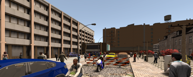
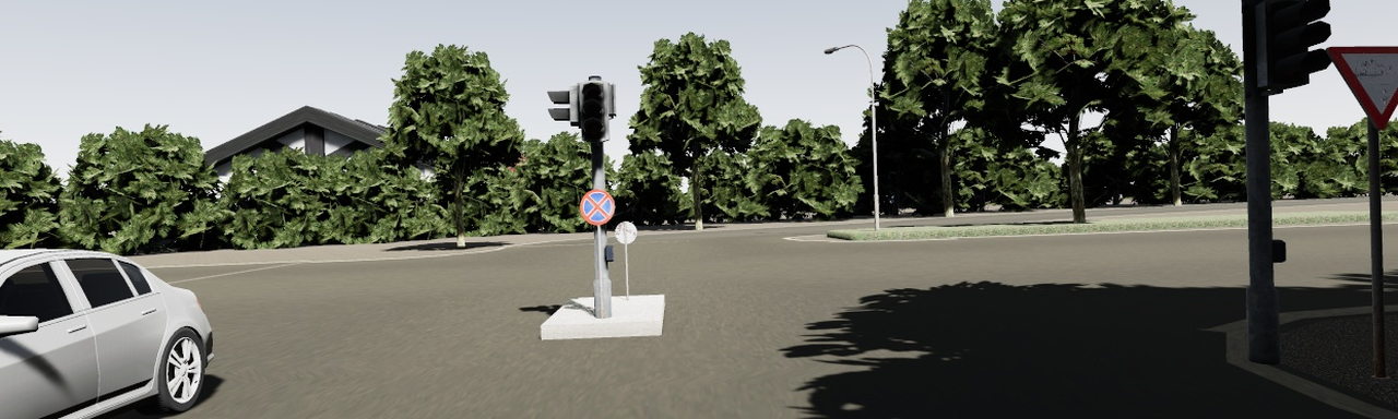
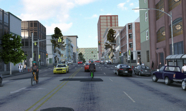
(a)

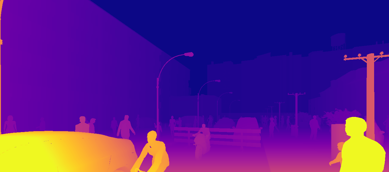
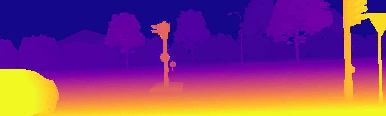
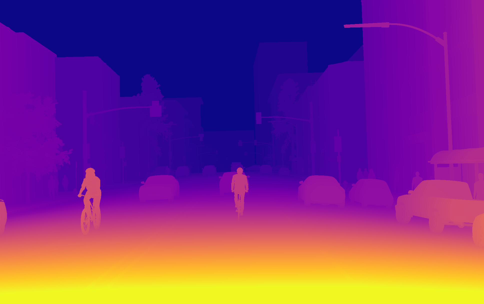
(b)

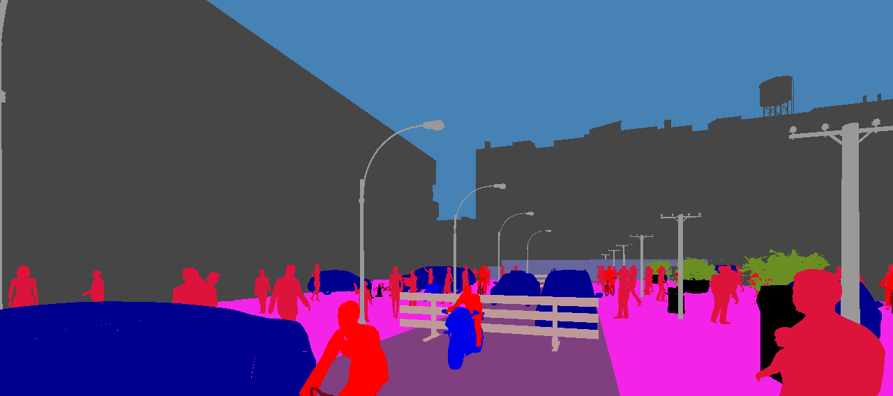
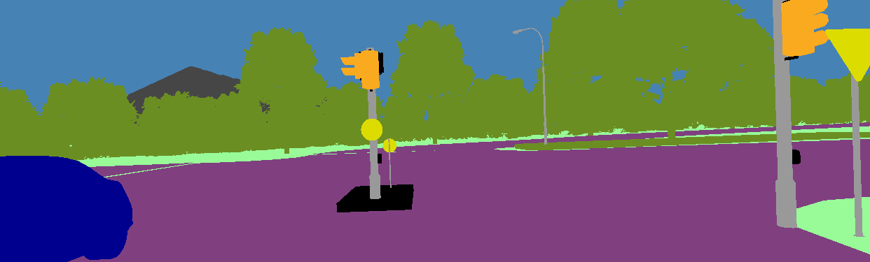
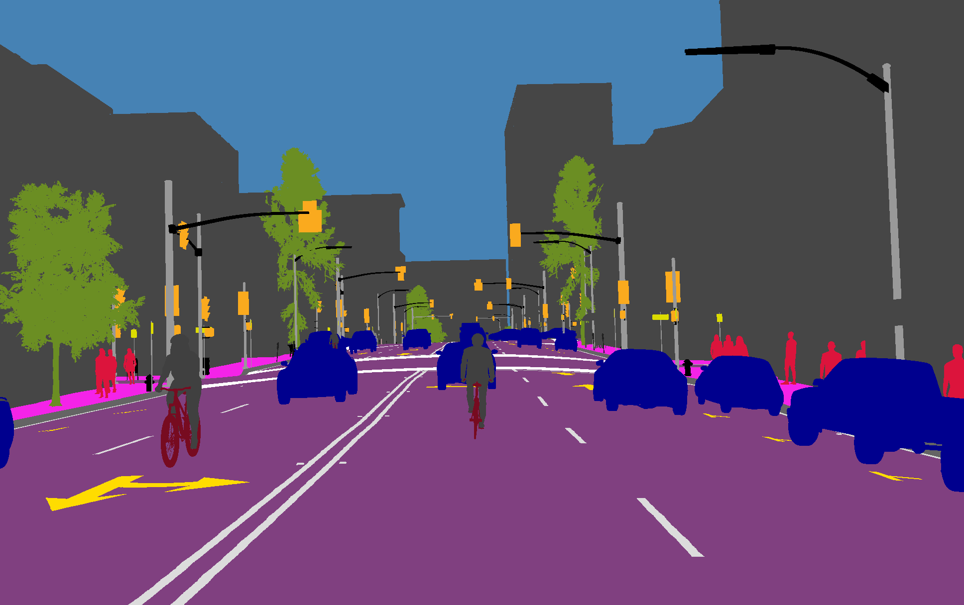
(a) Synthetic datasets (ground-truth)

Cityscapes              KITTI                DDAD

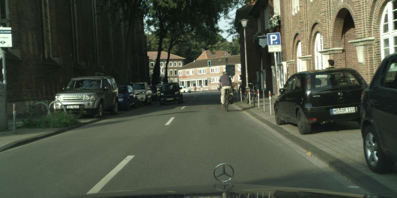
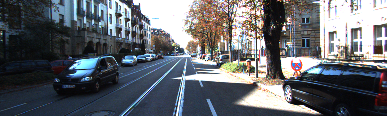
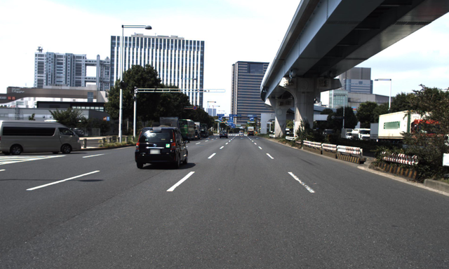
(b)

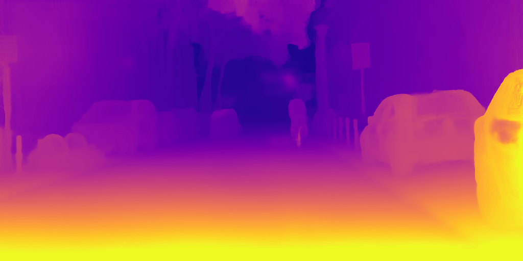
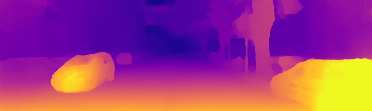
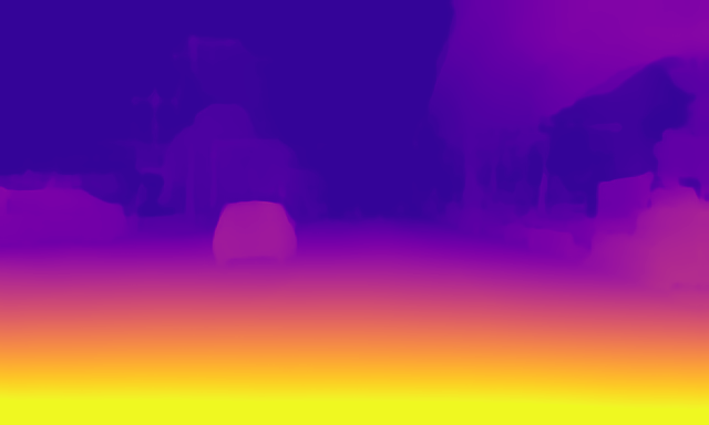
(c)

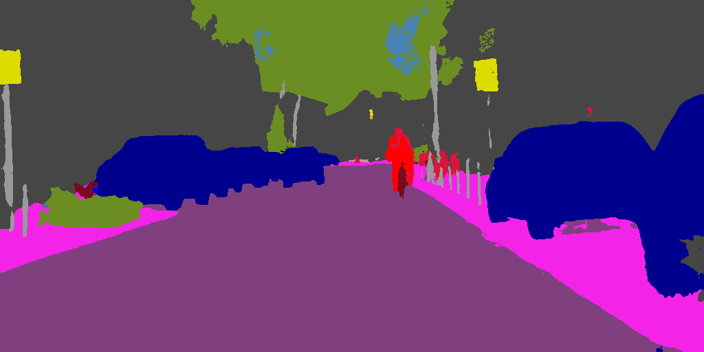
(b) Real-world datasets (predictions)

Figure 1: Our GUDA approach uses geometric self-supervision on videos in a multi-task setting to achieve state-of-the-art results in UDA for semantic segmentation.

Self-supervised learning from geometric constraints is used to learn tasks like depth and ego-motion directly from unlabeled videos [16, 26, 28, 56, 81]. However, tasks like semantic segmentation and object detection inherently require human-defined labels. A promising alternative to expensive manual labeling is to use synthetic datasets [4, 12, 17, 50, 51]. Simulators can indeed be programmed to generate large quantities of diverse data with accurate labels (cf. Fig. 1), including for optical and scene flow [34, 49], object detection [47], tracking [17], action recognition [12], and semantic segmentation [50, 51]. However, no simulator is perfect. Hence, effectively using synthetic data requires overcoming the sim-to-real domain gap, a distribution shift between a source synthetic domain and a target real one due to differences in content, scene geometry, physics, appearance, or rendering artifacts.

The goal of Unsupervised Domain Adaptation (UDA) is to improve generalization across this domain gap without any real-world labels. Most methods use adversarial learning for pixel or feature-level adaptation [3, 18, 31, 39, 59, 64, 74] or self-training by refining pseudo-labels [35, 36, 78, 82, 83, 55]. These methods yield clear improvements, but require learning multiple networks beyond the target one, are hard to train (adversarial learning), or limited to semantically close domains (iterative diffusion of high-confidence pseudo-labels). Alternatively, few works [58, 72] have explored simple image-level self-supervised proxy tasks [23, 44, 37] to improve generalization across domains, but with only limited success for UDA of semantic segmentation.

In this work, we introduce self-supervised monocular depth as a proxy task for UDA in semantic segmentation. We propose a multi-task mixed-batch training method combining synthetic supervision with a real-world self-supervised depth estimation objective to learn a domain-invariant encoder. Although it is not obvious that geometric constraints on videos can help overcome a semantic gap on images, our method, called GUDA for Geometric Unsupervised Domain Adaptation, outperforms other UDA methods for semantic segmentation. Furthermore, we can directly combine our method with self-trained pseudo-labels, leading to a new state of the art on the standard SYNTHIA-to-Cityscapes benchmark. In addition, we show on Cityscapes [10], KITTI [21], and DDAD [28] that our method scales well with both the quantity and quality of synthetic data (cf. Fig. 1), from SYNTHIA [51] to VKITTI2 [4], and a new large-scale high-quality dataset [1]. Finally, we show that GUDA is also capable of state-of-the-art monocular depth estimation in the real-world domain.

2 Related Work

2.1 Unsupervised Domain Adaptation

Unsupervised domain adaptation (UDA) is an active research area in Computer Vision [11, 67, 69]. Its main goal is to learn a model on a labeled source dataset and a related but statistically different unlabeled target dataset where the model is expected to generalize. Common approaches rely on domain-invariant learning or statistical alignment between domains [18, 61, 73]. In this work, we consider UDA for semantic segmentation, for which the labeling process is tedious and expensive. Several synthetic datasets have been proposed to reduce the need for real-world labels, such as SYNTHIA [51], GTA5 [50], and Virtual KITTI [17].

However, models trained on such datasets suffer from a significant performance drop when tested on real-world datasets. To overcome this large sim-to-real generalization gap, several works have proposed to use adversarial learning for distribution alignment at the level of pixels [31, 70, 75, 76, 74], features [32, 53, 33], or outputs [60, 65, 54]. Alternatively, self-training (a.k.a. pseudo-labeling) has also been successful for UDA [83, 82, 57, 36, 78, 55]. In these works, models are iteratively trained with both ground truth labels in the source domain and inferred pseudo-labels in the target domain, updated as part of an optimization loop.

Although still underexplored, another promising direction is the use of other modalities in the source domain to help the unsupervised transfer of semantic segmentation to the target domain. SPIGAN [39] uses synthetic depth as privileged information to provide additional regularization during adversarial training. GIO-Ada [8] uses geometric information, including depth and surface normals, during style-transfer in the target domain. DADA [66] predicts depth and semantic segmentation during adversarial training using a shared encoder, and fuses depth-aware features to improve semantic segmentation predictions.

In contrast to [8, 39, 66], we do not only use source depth information as explicit supervision or to enforce additional constraints during the adaptation stage. Instead, we infer and leverage depth in the target domain through self-supervision from geometric video-level cues, and use it as the primary source of domain adaptation. By simultaneously learning depth estimation in both domains, we produce features that are discriminative enough to perform this task while being robust to general differences in distribution between target and source domains.

2.2 Self-Supervised Learning

Self-supervised learning (SSL) has recently shown promising results in feature extraction through the definition of auxiliary tasks, using only unlabeled data as input [23, 37, 44, 62]. Typical auxiliary tasks look at different ways of reconstructing input data, such as rotation [23], patch jigsaw puzzles [44], or image colorization [37]. Only few works have used SSL as a tool for domain adaptation [22, 5, 58, 72], reporting results far from the state of the art (cf. Tab. 1). [22] proposes an auxiliary image reconstruction task on the target domain for image classification [22], whereas [5, 58, 72] explore different image-level pretext tasks to improve standard adversarial domain adaptation.

In this paper, we build upon recent developments in self-supervised learning in videos for monocular depth and ego-motion estimation [26, 28, 56, 79]. We show that these SSL tasks help UDA, leveraging strong geometric priors from videos to adapt features in a multi-task setting.

3 Geometric Unsupervised Adaptation

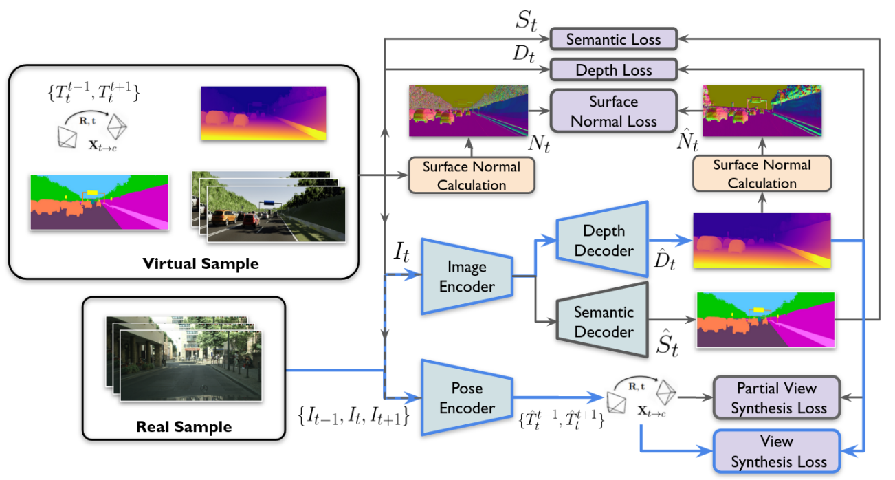
Figure 2: Diagram of our proposed multi-task multi-domain GUDA architecture for geometric unsupervised domain adaptation using mixed-batch training of real (Sec. 3.1) and virtual (Sec. 3.2) samples. The common paths during training (self-supervised) are in blue, whereas other ones (gray) use synthetic supervision.

A diagram of our proposed architecture for geometric unsupervised domain adaptation (GUDA) is shown in Fig. 2. It is composed of three networks: Depth $f_{D}:I\rightarrow\hat{D}$, that takes an input image $I$ and outputs a predicted depth map $\hat{D}$; Semantic $f_{S}:I\rightarrow\hat{S}$, that takes the same input image and outputs a predicted semantic map $\hat{S}$; and Pose $f_{T}:\{I_{a},I_{b}\}\rightarrow\hat{T}_{a}^{b}$, that takes a pair of images and outputs the rigid transformation $\hat{T}$ between them. The depth and semantic networks share the same encoder $f_{E}:I\rightarrow\hat{F}$, such that $f_{D}:f_{E}(I)\rightarrow\hat{D}$ and $f_{S}:f_{E}(I)\rightarrow\hat{S}$ both decode the same latent features $\hat{F}$ into their respective tasks. See Sec. 4.2 for architecture details.

During training we employ a mixed-batch approach, in which at each iteration real $\mathcal{B}_{R}$ and virtual $\mathcal{B}_{V}$ batches are received and processed to generate corresponding real $\mathcal{L}_{R}$ (Sec. 3.1) and virtual $\mathcal{L}_{V}$ (Sec. 3.2) losses, depending on the available information. The final loss is defined as:

$$\mathcal{L}=\mathcal{L}_{R}+\lambda_{V}\mathcal{L}_{V}$$ (1)

where $\lambda_{V}$ is a coefficient used to balance real and virtual losses during optimization. The next sections detail how each of these losses is calculated.

3.1 Real (Target) Sample Processing

Real-world samples are assumed to contain only unlabeled image sequences $\mathcal{I}_{t}$, in the form of the current frame $I_{t}$ and a temporal context $\{I_{t-s},\cdots,I_{t+s}\}$. In all experiments we considered a temporal context of $s=1$, resulting in $\mathcal{I}_{t}=\{I_{t-1},I_{t},I_{t+1}\}$. For simplicity, we also assume known and constant camera intrinsics $K$ for all frames, however this assumption can be relaxed to include the simultaneous learning of the projection model [27, 63]. Following [58], we use an auxiliary self-supervised task in the target domain to help adapt features learned in the source domain. Specifically, depth and ego-motion learning via self-supervised photometric consistency in videos has been shown to produce results competitive with supervised learning in some domains [28, 79]. Leveraging this insight, we define our target domain loss as:

$$\mathcal{L}_{R}=\mathcal{L}_{P}+\lambda_{PL}\mathcal{L}_{PL}$$ (2)

where $\mathcal{L}_{P}$ is the self-supervised photometric loss described in Section 3.1.1, and $\mathcal{L}_{PL}$ is an optional pseudo-label loss described in Section 3.1.2, with weight coefficient $\lambda_{PL}$.

3.1.1 Self-Supervised Photometric Loss

Following previous works [19, 79], the self-supervised depth and ego-motion objective can be formulated as a novel view synthesis problem, in which a target image $I_{t}$ is reconstructed using information from a reference image $I_{t^{\prime}}$ given a predicted depth map $\hat{D}_{t}$ and relative transformation $T_{t}^{t^{\prime}}$ between images:

$$\hat{I}_{t}=I_{t^{\prime}}\Big{\langle}\pi\Big{(}\hat{D}_{t},\hat{T}^{t^{\prime}}_{t},K\Big{)}\Big{\rangle}$$ (3)

where $\pi$ is the projection operation determined by camera geometry and $\langle\rangle$ is the bilinear sampling operator, that is locally sub-differentiable and thus can be used as part of an optimization pipeline. To measure the reconstruction error we use the standard photometric loss [77], with a structural similarity (SSIM) component [68] and the L1 distance in pixel space, weighted by $\alpha=0.85$:

$$\small\mathcal{L}_{P}(I_{t},\hat{I}_{t})=\alpha\frac{\Big{(}1-\text{SSIM}(I_{t},\hat{I}_{t})\Big{)}}{2}+(1-\alpha)||I_{t}-\hat{I}_{t}||_{1}$$ (4)

This loss is calculated for every image $I_{t^{\prime}}\in\mathcal{I}_{t}$ and averaged for all pixels between multiple scales, after upsampling to the highest resolution. Following [26], we use auto-masking and minimum reprojection error to mitigate effects caused by occlusions and dynamic objects.

3.1.2 Pseudo-Label Distillation

Self-training methods [36, 78, 83] are currently the dominant framework to address unsupervised domain adaptation for several different tasks [52]. They work by iteratively refining high-confidence pseudo-labels in the target domain using supervision in the source domain. This source of domain adaptation can in principle be used to augment our proposed domain adaptation via geometric self-supervision.

Here we propose a simple yet effective way to distill information from self-training methods (or any other UDA method) into GUDA, by using pre-calculated pseudo-labels as supervision in the target domain. The resulting loss is similar to the supervised semantic loss described in Sec. 3.2.1, using the predicted semantic map $\hat{S}$ from the real sample and the pseudo-label $S^{PL}$ pre-calculated from the same input image $I$ as ground-truth:

$$\mathcal{L}_{PL}=\mathcal{L}_{S}(\hat{S},S^{PL})$$ (5)

In our ablation analysis (Tab. 2), we show that the combination of GUDA with pseudo-label supervision from a self-training method [78] achieves the best results, surpassing other methods and establishing a new state of the art in unsupervised domain adaptation for semantic segmentation.

3.2 Virtual (Source) Sample Processing

Virtual samples consist of input images $I_{t}$ with corresponding dense annotations for all considered tasks, i.e. depth maps $D_{t}$ and semantic labels $S_{t}$. If sequential data is available we also assume a temporal context $\mathcal{I}_{t}=\{I_{t-1},I_{t},I_{t+1}\}$, corresponding ground-truth rigid transformation between frames $\mathcal{T}_{t}=\{T_{t}^{t-1},T_{t}^{t+1}\}$, and constant camera intrinsics $K$. The availability of supervision allows the learning of both semantic and depth tasks in the source domain, encoding this information into the shared encoder $f_{E}$ and the respective decoders $f_{D}$ and $f_{S}$. We define our source domain loss as follows:

$$\mathcal{L}_{V}=\mathcal{L}_{D}+\lambda_{S}\mathcal{L}_{S}+\lambda_{N}\mathcal{L}_{N}+\lambda_{PP}\mathcal{L}_{PP}$$ (6)

where $\mathcal{L}_{S}$ is a supervised semantic loss (Sec. 3.2.1), $\mathcal{L}_{D}$ is a supervised depth loss (Sec. 3.2.2), $\mathcal{L}_{N}$ is a surface normal regularization term (Sec. 3.2.3), and $\mathcal{L}_{PP}$ is an optional partially-supervised photometric loss (Sec. 3.2.4), each weighted by their corresponding coefficient.

3.2.1 Supervised Semantic Loss

Following [71, 48], we supervise semantic segmentation in the source domain using a bootstrapped cross-entropy loss between predicted $\hat{S}$ and ground-truth $S$ labels:

$$\mathcal{L}_{S}=-\frac{1}{K}\sum_{u=1}^{H}\sum_{v=1}^{W}\sum_{c=1}^{C}\mathbbm{1}_{[c=y_{u,v},p_{u,v}^{c}<t]}\log\Big{(}p_{u,v}^{c}\Big{)}$$ (7)

where $p_{u,v}^{c}$ denotes the predicted probability of pixel $(u,v)$ belonging to class $c$. The term $t$ is a run-time threshold so that only the worst $K$ performing predictions are considered. We adopt $K=0.3\times H\times W$ in our experiments.

(a)

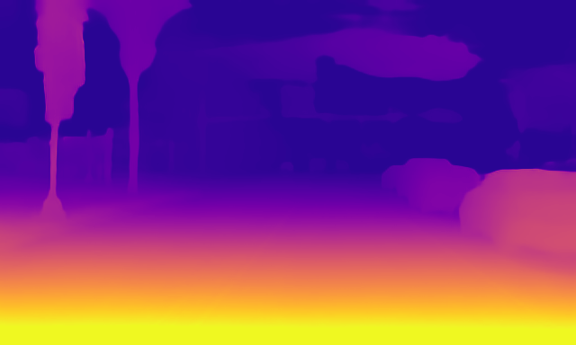
(b)

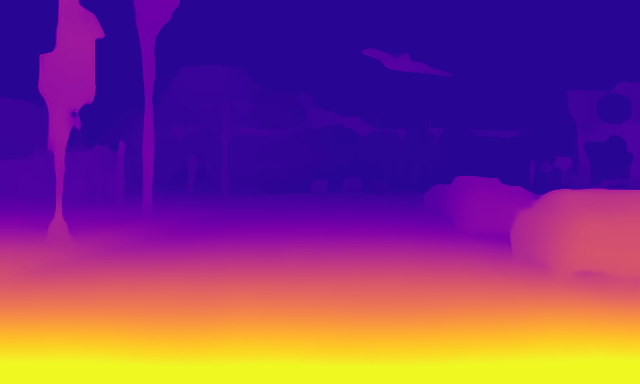
(c)

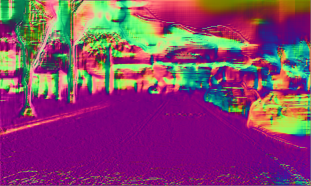
(a) Real-world
self-supervision

(b) Synthetic depth
supervision

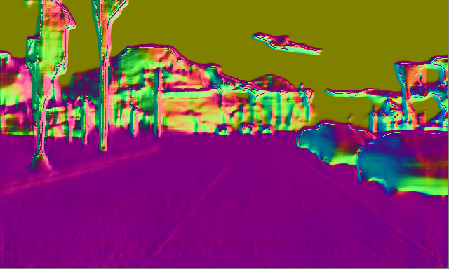
(c) Synthetic depth + normal supervision

Figure 3: Effects of surface normal regularization from synthetic datasets on a real-world sample. In (a) only self-supervision on the real images was used during training, in (b) a synthetic depth loss was added, and in (c) our proposed surface normal regularization loss was added.

3.2.2 Supervised Depth Loss

Our supervised objective loss is the Scale-Invariant Logarithmic loss (SILog) [15], composed by the sum of the variance and the weighted squared mean of the error in log space $\Delta d=\log d-\log\hat{d}$:

$$\mathcal{L}_{D}=\frac{1}{P}\sum_{d\in D}\Delta d^{2}-\frac{\lambda}{P^{2}}\left(\sum_{d\in D}\Delta d\right)^{2}$$ (8)

where $P$ is the number of pixels $d\in D$ with valid depth information. The coefficient $\lambda$ balances variance and error minimization, and following previous works [38] we use $\lambda=0.85$ in all experiments.

3.2.3 Surface Normal Regularization

Because depth estimates are produced on a per-pixel basis, it is common to enforce an additional smoothness loss [24] to maintain local consistency. Here we propose an alternative to the smoothness loss, that leverages the dense depth supervision available in synthetic datasets and minimizes instead the difference between surface normal vectors produced by ground-truth and predicted depth maps. Note that, differently from other methods [14, 43], we are not explicitly predicting surface normals as an additional task, but rather using them as regularization to enforce certain structural properties in the predicted depth maps. For any pixel $\mathbf{p}\in D$, its surface normal vector $\mathbf{n}\in\mathbb{R}^{3}$ is calculated as:

$$\mathbf{n}=\Big{(}\mathbf{P}_{u+1,v}-\mathbf{P}_{u,v}\Big{)}\times\Big{(}\mathbf{P}_{u,v+1}-\mathbf{P}_{u,v}\Big{)}$$ (9)

where $\mathbf{P}=\phi(\mathbf{p},d,K)$ is the point obtained by unprojecting $\mathbf{p}$ from the camera frame of reference into 3D space, given its depth value $d$ and intrinsics $K$. As a measure of proximity between two surface normal vectors we use the cosine similarity metric, defined as:

$$\mathcal{L}_{N}=\frac{1}{2P}\sum_{\mathbf{p}\in D}\Big{(}1-\frac{\hat{\mathbf{n}}\cdot\mathbf{n}}{||\hat{\mathbf{n}}||\hskip 1.99997pt||\mathbf{n}||}\Big{)}$$ (10)

where $\mathbf{n}$ and $\hat{\mathbf{n}}$ are unitary vectors representing respectively ground-truth and predicted surface normals for each pixel $\mathbf{p}\in D$. In Fig. 3 we show the impact that our proposed surface normal regularization has in the resulting predicted depth maps. While pure self-supervision on the target domain produces accurate depth maps, the surface normals are locally inconsistent and fail to properly capture object geometry. Introducing synthetic depth supervision significantly improves consistency, and our proposed regularization further sharpens object boundaries and enables the proper modeling of far away areas, including the sky.

3.2.4 Partially-Supervised Photometric Loss

If image sequences are also provided as part of the synthetic sample, we can use the same self-supervised photometric loss described in Sec. 3.1.1 as additional training signal for the depth and pose networks. Furthermore, because we have individual dense depth and pose supervision, we can decouple each task within the self-supervised photometric loss. This is achieved by modifying Eq. 3 to define $\hat{I}_{t}^{D}=I_{t^{\prime}}\Big{\langle}\pi\Big{(}D_{t},\hat{T}^{t^{\prime}}_{t},K\Big{)}\Big{\rangle}$ as the reconstructed target image obtained using ground-truth depth and predicted pose. Similarly, we can define $\hat{I}_{t}^{T}=I_{t^{\prime}}\Big{\langle}\pi\Big{(}\hat{D}_{t},T^{t^{\prime}}_{t},K\Big{)}\Big{\rangle}$ as the reconstructed target image obtained using predicted depth and ground-truth pose. The final partially-supervised photometric loss is calculated as:

$$\mathcal{L}_{PP}=\frac{1}{3}\Big{(}\mathcal{L}_{P}(I_{t},\hat{I}_{t})+\mathcal{L}_{P}(I_{t},\hat{I}_{t}^{D})+\mathcal{L}_{P}(I_{t},\hat{I}_{t}^{T})\Big{)}$$ (11)

4 Experimental Protocol

4.1 Implementation Details

Our models are implemented using Pytorch [46] and trained across eight V100 GPUs with a batch size $b=8$ (1 per GPU) for both source and target datasets. The shared depth and semantic encoder takes as input one RGB image (the middle frame), and the pose network takes three consecutive RGB images. We use the Adam optimizer [41], with $\beta_{1}=0.9$, $\beta_{2}=0.999$, and starting learning rate $lr=10^{-4}$. The length of each epoch is determined by the target dataset, and at each iteration samples are randomly selected from both source and target datasets. Our training schedule consists of $20$ epochs at half resolution, followed by $20$ epochs at full resolution, halving the learning rate for the final $10$ epochs. This multi-scale schedule is used to increase convergence speed and has no meaningful impact in final model performance, as shown in Tab. 2. If pseudo-labels are available, the model is refined for another $10$ epochs with the introduction of $\mathcal{L}_{PL}$, halving the learning rate for the final $5$ epochs. Through grid search we have determined the loss coefficients to be $\lambda_{V}=1$, $\lambda_{S}=0.001$, $\lambda_{N}=0.01$, $\lambda_{PP}=0.005$ and $\lambda_{PL}=0.01$. Results are stable, starting to vary with coefficient changes of around one order of magnitude.

4.2 Networks

Unless noted otherwise, we use a ResNet101 [30] with ImageNet [13] pre-trained weights as the shared backbone for the semantic and depth decoders. The depth decoder follows [26] and outputs inverse depth maps at four different resolutions. The semantic decoder is similar and outputs semantic logits at a single resolution, obtained by concatenating the four output scales (upsampled to the highest resolution) followed by a final convolution layer. Our pose network also follows [26] and uses a ResNet18 encoder (also pre-trained on ImageNet), followed by a series of convolutions that output a 6-dimensional vector containing translation and rotation in Euler angles. For more details we refer the reader to the supplementary material.

4.3 Datasets

4.3.1 Real Datasets

Cityscapes [10]

The Cityscapes dataset is a widely used benchmark for semantic segmentation evaluation. For self-supervision on the target domain, following [28], we use the $2975$ training images (without the labels) with their corresponding $30$-frame sequences, for a total of $2975\times 30=89250$ images. In Tab. 2 we ablate the impact of training with fewer frames, such as 2-frame sequences (the minimum required for monocular self-supervised learning). We evaluate our semantic segmentation performance on the official $500$ annotated validation set.

KITTI [20]

The KITTI dataset is considered the standard benchmark for depth evaluation. We use the Eigen split filtered according to [80], resulting in 39810 training, 888 validation and 697 test images, with corresponding LiDAR-projected depth maps (used only for evaluation). To evaluate semantic segmentation we use the 200 annotated frames found in [2], mapped to the Cityscapes ontology [10].

DDAD [28]

The Dense Depth for Automated Driving dataset is a challenging depth evaluation benchmark, with denser ground-truth depth maps and longer ranges of up to 250m. We consider only the front camera, resulting in $150$ training sequences with $12560$ images and $50$ validation sequences with $3950$ images, from which $50$ are semantically labeled (the middle frame in each sequence).

Method	Sty.Trans.	Advers.	Depth	Self-Sup.	Ps.-Label	mIoU	mIoU*
Source (SY)						31.7	36.7
Source (PD)						38.1	44.0
Target						72.9	77.8
(a) SYNTHIA $\rightarrow$ Cityscapes
SPIGAN [39]	✓	✓	✓			36.8	42.4
GIO-Ada [8]	✓	✓	✓			37.3	43.0
DADA [66]		✓	✓			42.6	49.8
GUDA			✓	✓		44.5	50.9
CLAN [42]		✓				—	47.8
Xu et al.[72]		✓		✓		38.8	—
CBST [83]					✓	42.5	48.4
CRST [82]					✓	43.8	50.1
ESL [55]					✓	43.5	50.7
FDA [75]	✓					—	52.5
CCMD [40]					✓	45.2	52.6
Yang el al. [74]	✓	✓				—	53.1
USAMR [78]				✓	✓	46.5	53.8
IAST [36]					✓	49.8	57.0
GUDA+PL			✓	✓	✓	51.0	57.9
(b) Varying Sources (G5, PD) $\rightarrow$ Cityscapes
UDAS (G5) [58]	✓	✓		✓		44.3	49.2
USAMR (G5) [78]				✓	✓	53.1	58.0
IAST (G5) [36]					✓	55.6	61.2
GUDA(PD)+PL(G5)			✓	✓	✓	57.2	63.2

Table 1: Semantic segmentation results on Cityscapes using different unsupervised domain adaptation (UDA) methods and synthetic datasets. mIoU considers all 16 classes, and mIoU* only the 13 SYNTHIA classes. Source shows results without any adaptation, and Target shows results with semantic supervision on the target domain. Synthetic datasets include: SYNTHIA (SY), Parallel Domain (PD), and GTA5 (G5). Detailed per class results are given in the supplementary material.

4.3.2 Synthetic Datasets

SYNTHIA [51]

The SYNTHIA dataset contains scenes generated from an autonomous driving simulator of urban scenes. For a fair comparison with other methods we used the SYNTHIA-RAND-CITYSCAPES subset, with $9400$ images and semantic labels compatible with Cityscapes.

VKITTI2 [4]

The VKITTI2 dataset was recently released as a more photo-realistic version of [17], containing reconstructions of five sequences found in the KITTI odometry benchmark [21] for a total of $2156$ samples.

Parallel Domain [1]

The Parallel Domain dataset is procedurally-generated and contains fully annotated photo-realistic renderings of urban driving scenes, including multiple cameras and LiDAR sensors. It contains $5000$ $10$-frame sequences, with $4200$/$800$ training and validation splits. More details and examples can be found in the supplementary material.

GTA5

[50] The GTA5 dataset is a street view synthetic dataset rendered from the GTA5 game engine, containing $24966$ images and semantic labels defined on $19$ classes compatible with Cityscapes.

5 Experimental Results

5.1 Semantic Segmentation

First, we evaluate our proposed GUDA framework on the task of unsupervised domain adaptation for semantic segmentation using the Cityscapes dataset. We consider three different scenarios, with results shown in Tab. 1. In (a) we use the SYNTHIA dataset as source and compare against other methods that use depth in the source domain as additional supervision, either as regularization [39], to reduce domain shift at different feature levels [8], or by sharing a lower-level representation like us. From these results, we see that GUDA outperforms all previous methods, even though it does not leverage additional translation networks or adversarial training. These results confirm that training the depth network in both domains thanks to self-supervised geometric constraints on target videos improves the generalization of the shared intermediate representation.

A more detailed analysis (available in the supplementary material) shows that GUDA excels in classes with well-defined geometries, such as road, sidewalk, and building. Interestingly, it also performs well on sky, most likely due to our proposed surface normal regularization (Sec. 3.2.3), which can properly model such areas (Fig. 3). We also note that GUDA’s smallest improvements are on rarer dynamic classes (e.g., motorcycle). This stems from the photometric loss being unable to model dynamic object motion due to a static world assumption [26, 29].

To overcome this limitation, we introduce pseudo-label supervision (Sec. 3.1.2) from USAMR [78], obtained by evaluating the official pre-trained model (mIoU 46.5) on our 89250 training images. In this configuration, GUDA achieves state-of-the-art results, outperforming UDA methods relying on style-transfer [75, 74], adversarial learning [42], self-training [83, 36, 40, 55], or other forms of (non-geometric) self-supervision [72, 58]. Fig. 4 analyzes the interplay between geometric self-supervision (GS) and pseudo-labels (PL), indicating an optimal pseudo-labeling loss weight $\lambda_{PL}=0.01$.

A detailed ablation study of our proposed architecture can be found in Tab. 2. It shows that (i) geometric supervision by itself improves performance, (ii) all components help, and (iii) the benefits of our method are not due simply to using more target data (video frames), although GUDA can benefit from them in contrast to other approaches.

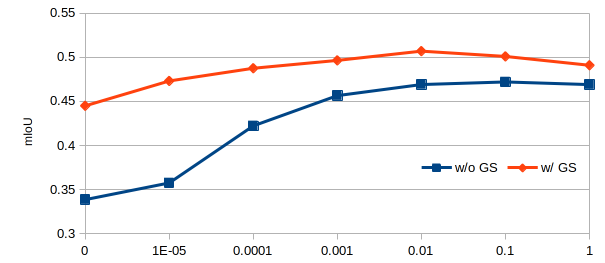
Figure 4: Effects of pseudo-label supervision, with and without our proposed geometric self-supervision (GS) for different values of $\lambda_{PL}$. When GS is not used (blue line), there is no benefit in adding virtual supervision, and as $\lambda_{PL}$ increases results converge to those using only pseudo-label supervision (Tab. 2). When GS is used (red line), results are consistently higher and start to degrade after $\lambda_{PL}=0.01$.

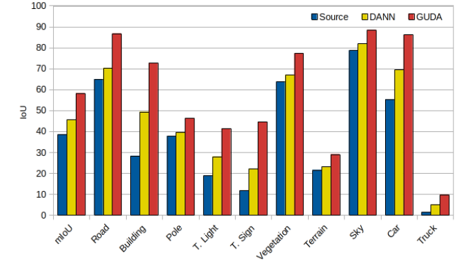
Figure 5: Semantic segmentation results on VKITTI2 $\rightarrow$ KITTI, using GUDA and DANN [18]. Detailed numbers are available in the supplementary material.

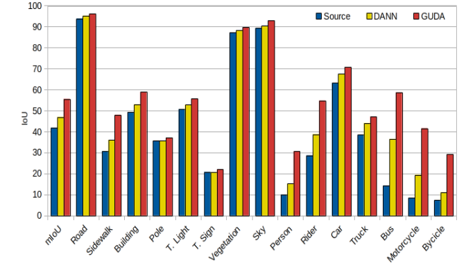
Figure 6: Semantic segmentation results on Parallel Domain $\rightarrow$ DDAD, using GUDA and DANN [18]. Detailed numbers are available in the supplementary material.

Finally, in Tab. 1 (b) we present results considering different source datasets. Because GTA5 [50] does not provide depth labels, we instead report results using the photorealistic Parallel Domain dataset, with GTA5 pseudo-labels (mIoU 53.1) from USAMR [78]. In this configuration, GUDA once more outperforms other considered methods, improving upon the state of the art when different source datasets are considered.

Variation	Real			Virtual
	GT	GS	PL	D	S	N	mIoU	mIoU*
DADA							42.6	49.8
DADA (2 frames)							42.5	49.3
DADA (30 frames)							42.4	49.5
Source only					✓		32.1	37.2
Target only (GT)	✓						73.9	78.7
Target only (PL)			✓				47.1	54.3
Virtual only				✓	✓	✓	33.8	38.8
GUDA - N		✓		✓	✓		43.4	48.0
GUDA (2 frames)		✓		✓	✓	✓	43.8	50.5
GUDA (single res.)		✓		✓	✓	✓	44.3	50.8
GUDA		✓		✓	✓	✓	44.5	50.9
GUDA + DANN		✓		✓	✓	✓	44.8	51.1
GUDA + PL - GS			✓	✓	✓	✓	46.8	54.1
GUDA + PL		✓	✓	✓	✓	✓	51.0	57.9

Table 2: Ablation study of our proposed method (SYNTHIA $\rightarrow$ Cityscapes). In the Real columns, GT refers to the use of ground-truth semantic labels, PL to the use of USAMR [78] semantic pseudo-labels (Sec. 3.1.2), and GS to the use of geometric self-supervision (Sec. 3.1.1). In the Virtual columns, D, S, and N refer respectively to semantic, depth, and surface normal supervision (Sec. 3.2). DANN refers to the use of an additional domain adversarial loss [18], and single res. to training only in full resolution. We also provide DADA results trained using 2 and 30 context frames (rather than 1), as well as GUDA results using only the minimum 2 context frames (rather than 30).

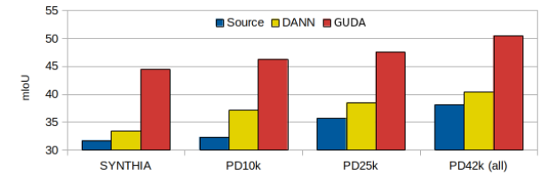
Figure 7: Performance improvement on Cityscapes with increasing data quality (SYNTHIA $\rightarrow$ PD) and quantity.

To evaluate how GUDA generalizes to other source and target datasets, we also provide semantic segmentation results from VKITTI2 to KITTI (Fig. 5) and Parallel Domain to DDAD (Fig. 6). To our knowledge, no current method reports results on these benchmarks for this task. Hence, we compare to the standard Domain Adversarial Neural Network (DANN) baseline [18], which uses a gradient reversal layer to learn discriminative features for the main task on the source domain while maximizing domain confusion.

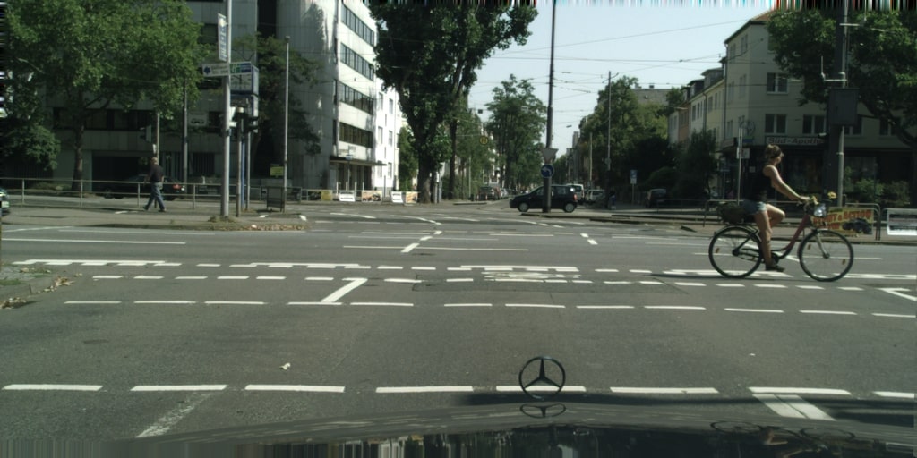
(a)

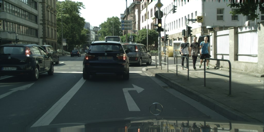
(b)

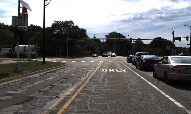
(c)

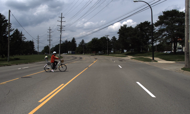
(d)

(e)

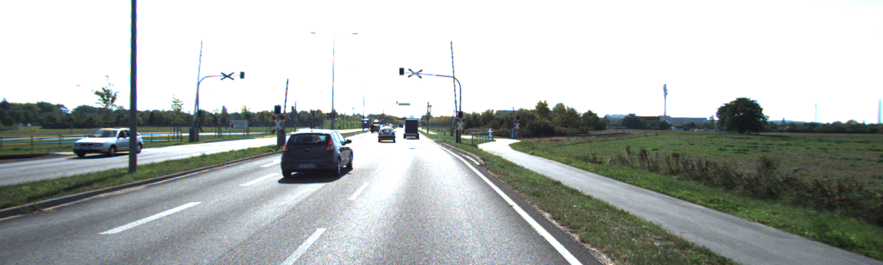
(f)

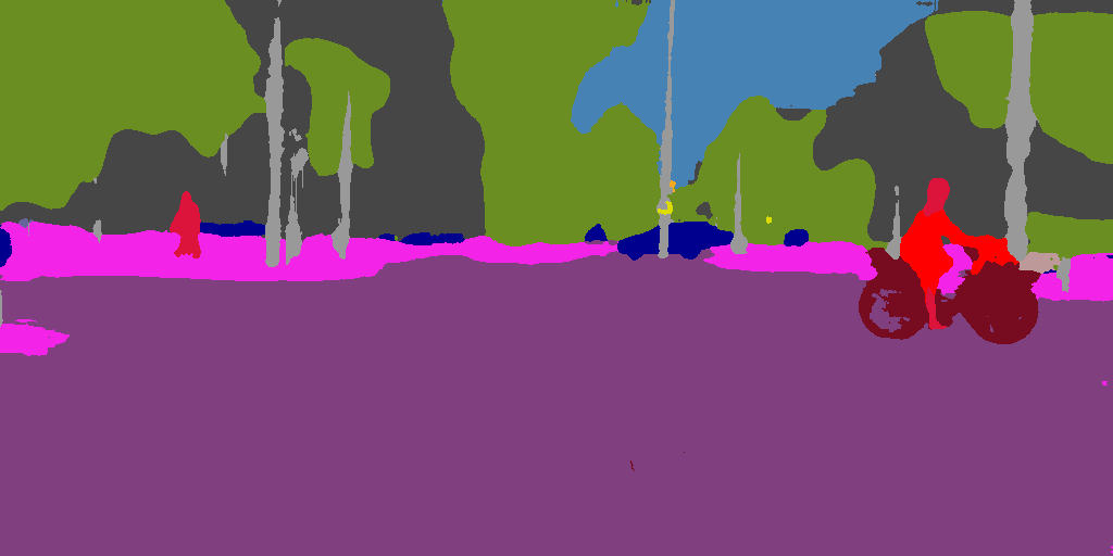
(g)

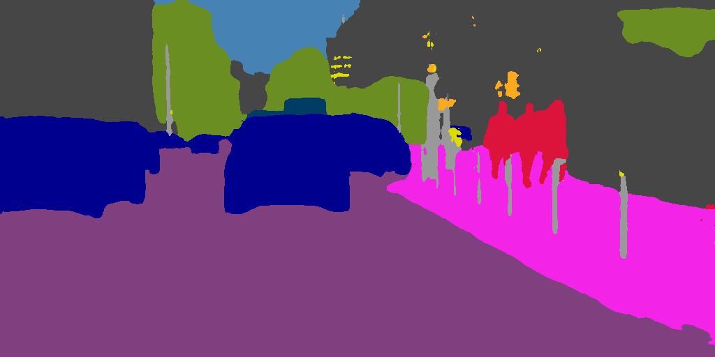
(h)

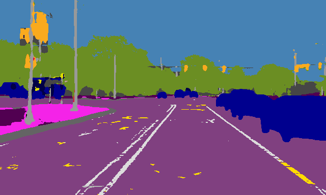
(i)

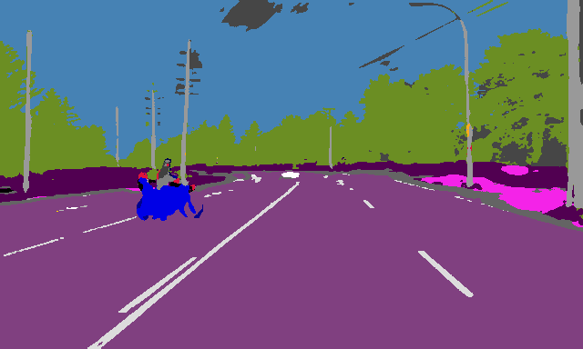
(j)

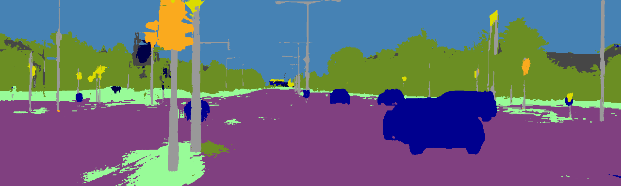
(k)

(l)

Figure 8: GUDA semantic segmentation results on Cityscapes, DDAD and KITTI.

	Method	Abs.Rel$\downarrow$	Sqr.Rel$\downarrow$	RMSE$\downarrow$	$\delta<1.25$$\uparrow$
KITTI	Source only$\dagger$ (R18)	0.191	2.078	7.233	0.699
	Target only (R18)	0.117	0.811	4.902	0.867
	Fine-tune (R18)	0.114	0.800	4.855	0.871
	GUDA$\dagger$ (R18) - PS	0.114	0.875	4.808	0.871
	GUDA$\dagger$ (R18)	0.109	0.762	4.606	0.879
	GUDA$\dagger$	0.107	0.714	4.421	0.883
DDAD	Source only$\dagger$ (R18)	0.233	7.429	18.498	0.620
	Target only (R18)	0.203	6.999	16.844	0.748
	Fine-tune (R18)	0.173	4.846	16.025	0.747
	GUDA$\dagger$ (R18) - PS	0.166	3.556	16.004	0.769
	GUDA$\dagger$ (R18)	0.158	3.332	15.112	0.778
	GUDA$\dagger$	0.147	2.922	14.452	0.809

Table 3: Depth estimation results on KITTI and DDAD. R18 indicates a ResNet18 [30] backbone, Source only and Target only indicate only synthetic or real-world, and Fine-tune indicates synthetic pre-training followed by real-world fine-tuning. PS indicates the removal of the partially-supervised photometric loss (Sec. 3.2.4). The symbol $\dagger$ indicates a scale-aware model (no test-time median-scaling).

As expected, DANN improves over source-only results by a significant margin ($+7.0/+5.1$ mIoU). Nevertheless, the stronger geometric supervision from GUDA still substantially outperforms DANN ($+12.65/+8.58$ mIoU), with similar trends as observed in previous experiments. In Fig. 7 we show how GUDA and DANN scale with improvements in data quality (from SYNTHIA to Parallel Domain) and data quantity (different subsets of Parallel Domain). Assuming linear improvement, GUDA would only require 200k synthetic samples to fully overcome the domain gap, whereas DANN would require 350k samples. We also show in Tab. 2 that GUDA and DANN can be combined, resulting in a $+0.2/0.3\%$ improvement.

5.2 Depth Estimation

As stated previously, GUDA achieves domain adaptation by jointly learning depth features in both domains, using a combination of dense synthetic supervision and geometric self-supervision on real-world images. To further demonstrate this property, in this section we analyze how GUDA impacts the task of monocular depth estimation itself and improves upon the standard approach of model fine-tuning. Similar to previous experiments, we evaluate on VKITTI2 to KITTI and Parallel Domain to DDAD, noting that each of these combinations have similar sensor configuration (intrinsics and extrinsics), which makes them particularly suitable for domain adaptation experiments. The same training schedule and architecture was used, with the inclusion of experiments using a ResNet18 backbone to facilitate comparison with other methods.

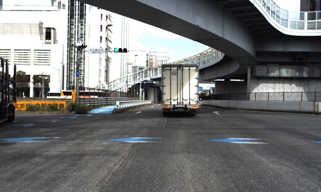
(a)

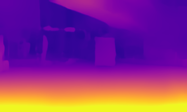
(b)

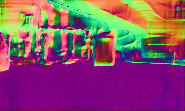
(c)

(d)

(e)

(f)

(g)

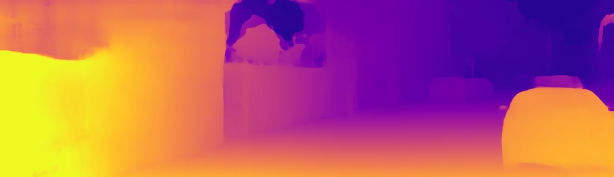
(h)

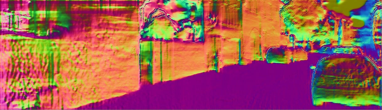
(i)

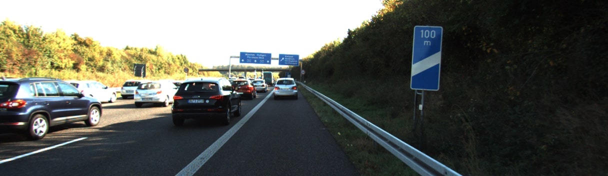
(a) Input image

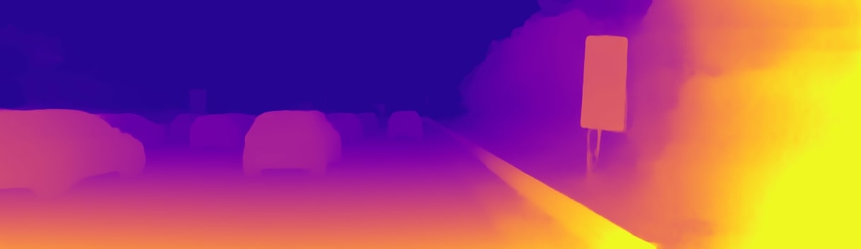
(b) Pred. depth

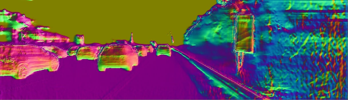
(c) Pred. normals

Figure 9: GUDA depth estimation results on KITTI and DDAD. Our proposed mixed-batch training schedule produces much sharper and consistent depth maps, especially at longer ranges and in “invalid” areas such as the sky.

Quantitative results are shown in Tab. 3, with qualitative examples in Fig. 9. The first noticeable aspect is that direct transfer (Source only) not only produces relatively accurate, but also scale-aware results, due to similarities in vehicle extrinsics and camera parameters. As expected, this behavior is not observed when only real-world information (Target only) is used, however it is also not observed when fine-tuning, indicating a catastrophic forgetting of the scale factor. In contrast, and although not our primary goal, GUDA preserves the scale learned from synthetic supervision and also significantly improves depth estimation performance relative to the standard fine-tuning approach. In alignment with recent observations [28], switching to a larger backbone improves results even further.

6 Conclusion

We introduce self-supervised monocular depth estimation as a proxy task for unsupervised sim-to-real transfer of semantic segmentation models. Our Geometric Unsupervised Domain Adaptation method, GUDA, combines dense synthetic labels with self-supervision from real-world unlabeled videos to bridge the sim-to-real domain gap. Although depth estimation is fundamentally a geometric task, we show it improves semantic representation transfer without any real-world semantic labels. Our multi-task self-supervised method outperforms other UDA approaches, while also improving monocular depth estimation. Furthermore, by introducing self-trained pseudo-labels as an extra source of supervision, we establish a new state of the art on this task. Finally, we show that our method scales well with both the quantity and quality of synthetic data, highlighting its potential to eventually close the sim-to-real gap in challenging visual conditions like driving scenes.

Appendix A Network Architectures

In Tab. 4 we describe in details the shared depth and semantic segmentation network used in our experiments. This architecture is based on recent developments in monocular depth estimation [26]. Note that our proposed algorithm can be generalized to any multi-scale backbones. We leave the exploration of architectures more suitable to jointly predict semantic segmentation [6, 7, 45] and monocular depth [26, 25] for future work. For the shared backbone we use a ResNet101 [30] encoder, that produces feature maps with varying number of channels at increasingly lower resolutions (#1, #2, #3, #4, #5 in Tab. 4). These feature maps are used as skip connections for both the depth and the semantic segmentation decoders, through a series of convolutional layers followed by bilinear upsampling. For the depth decoder, at the final four upsampling stages (#10, #13, #16, #19 in Tab. 4) an inverse depth layer is used to produce estimates within a minimum and maximum depth range:

$$\frac{1}{d_{u,v}}=\frac{1}{d_{max}}+\Big{(}\frac{1}{d_{min}}-\frac{1}{d_{max}}\Big{)}Sigmoid(f_{u,v})$$ (12)

All four scales are used to calculate the self-supervised photometric loss (with results averaged per-batch, per-scale and per-pixel), and only the final scale is used to calculate the supervised depth loss. During inference, only the final scale is used as depth prediction estimates. The semantic network is similar, with the difference that the outputs at each of the upsampling stages (#9, #11, #13, #15 in Tab. 4) are instead concatenated (after bilinear upsampling to the highest resolution) and processed using a final convolutional layer to produce a $C$-dimensional logits vector for each pixel.

	Layer Description	Out. Dimension
	RGB image	3$\times$H$\times$W
ResNet101 Encoder
#1	Intermediate Features #1	256$\times$H/2$\times$W/2
#2	Intermediate Features #2	256$\times$H/4$\times$W/4
#3	Intermediate Features #3	512$\times$H/8$\times$W/8
#4	Intermediate Features #4	1024$\times$H/16$\times$W/16
#5	Latent Features	2048$\times$H/32$\times$W/32
Depth Decoder
#6	Conv2d (#5) $\rightarrow$ ELU $\rightarrow$ Upsample	256$\times$H/16$\times$W/16
#7	Conv2d (#6 $\oplus$ #4) $\rightarrow$ ELU	256$\times$H/16$\times$W/16
#8	Conv2d (#7) $\rightarrow$ ELU $\rightarrow$ Upsample	128$\times$H/8$\times$W/8
#9	Conv2d (#8 $\oplus$ #3) $\rightarrow$ ELU	128$\times$H/8$\times$W/8
#10	Conv2d (#9) $\rightarrow$ InvDepth	1$\times$H/8$\times$W/8
#11	Conv2d (#9) $\rightarrow$ ELU $\rightarrow$ Upsample	64$\times$H/4$\times$W/4
#12	Conv2d (#11 $\oplus$ #2) $\rightarrow$ ELU	64$\times$H/4$\times$W/4
#13	Conv2d (#12) $\rightarrow$ InvDepth	1$\times$H/4$\times$W/4
#14	Conv2d (#12) $\rightarrow$ ELU $\rightarrow$ Upsample	32$\times$H/2$\times$W/2
#15	Conv2d (#14 $\oplus$ #1) $\rightarrow$ ELU	32$\times$H/2$\times$W/2
#16	Conv2d (#15) $\rightarrow$ InvDepth	1$\times$H/2$\times$W/2
#17	Conv2d (#15) $\rightarrow$ ELU $\rightarrow$ Upsample	16$\times$H$\times$W
#18	Conv2d (#17) $\rightarrow$ ELU	16$\times$H$\times$W
#19	Conv2d (#18) $\rightarrow$ InvDepth	1$\times$H$\times$W
Semantic Decoder
#6	Conv2d (#5) $\rightarrow$ ELU $\rightarrow$ Upsample	256$\times$H/16$\times$W/16
#7	Conv2d (#6 $\oplus$ #4) $\rightarrow$ ELU	256$\times$H/16$\times$W/16
#8	Conv2d (#7) $\rightarrow$ ELU $\rightarrow$ Upsample	128$\times$H/8$\times$W/8
#9	Conv2d (#8 $\oplus$ #3) $\rightarrow$ ELU	128$\times$H/8$\times$W/8
#10	Conv2d (#9) $\rightarrow$ ELU $\rightarrow$ Upsample	64$\times$H/4$\times$W/4
#11	Conv2d (#10 $\oplus$ #2) $\rightarrow$ ELU	64$\times$H/4$\times$W/4
#12	Conv2d (#11) $\rightarrow$ ELU $\rightarrow$ Upsample	32$\times$H/2$\times$W/2
#13	Conv2d (#12 $\oplus$ #1) $\rightarrow$ ELU	32$\times$H/2$\times$W/2
#14	Conv2d (#13) $\rightarrow$ ELU $\rightarrow$ Upsample	16$\times$H$\times$W
#15	Conv2d (#14) $\rightarrow$ ELU	16$\times$H$\times$W
#16	Conv2d (#9 $\oplus$ #11 $\oplus$ #13 $\oplus$ #15)	C$\times$H$\times$W

Table 4: Depth and semantic segmentation multi-task network. We use a ResNet101 backbone as encoder, that outputs intermediate features at different resolutions. These intermediate features are used as skip connections in different stages of the semantic and depth decoders. ELU are Exponential Linear Units [9], Upsample denotes bilinear interpolation, InvDepth is an inverse depth layer (Eq. 12), and $\oplus$ denotes feature concatenation.

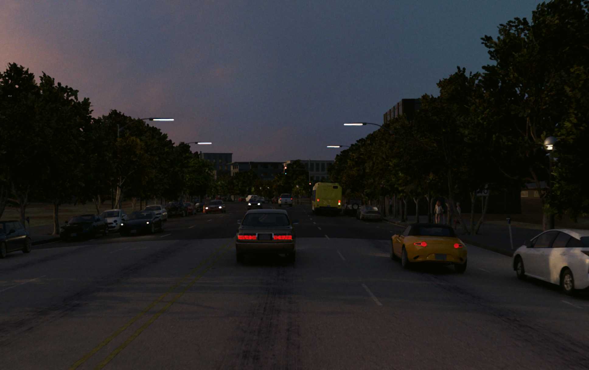
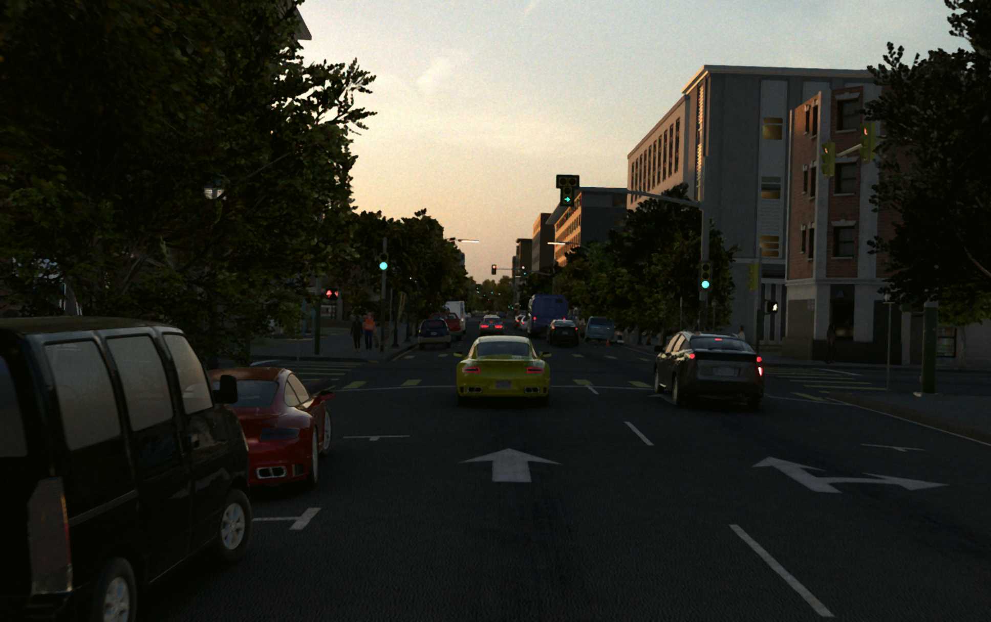
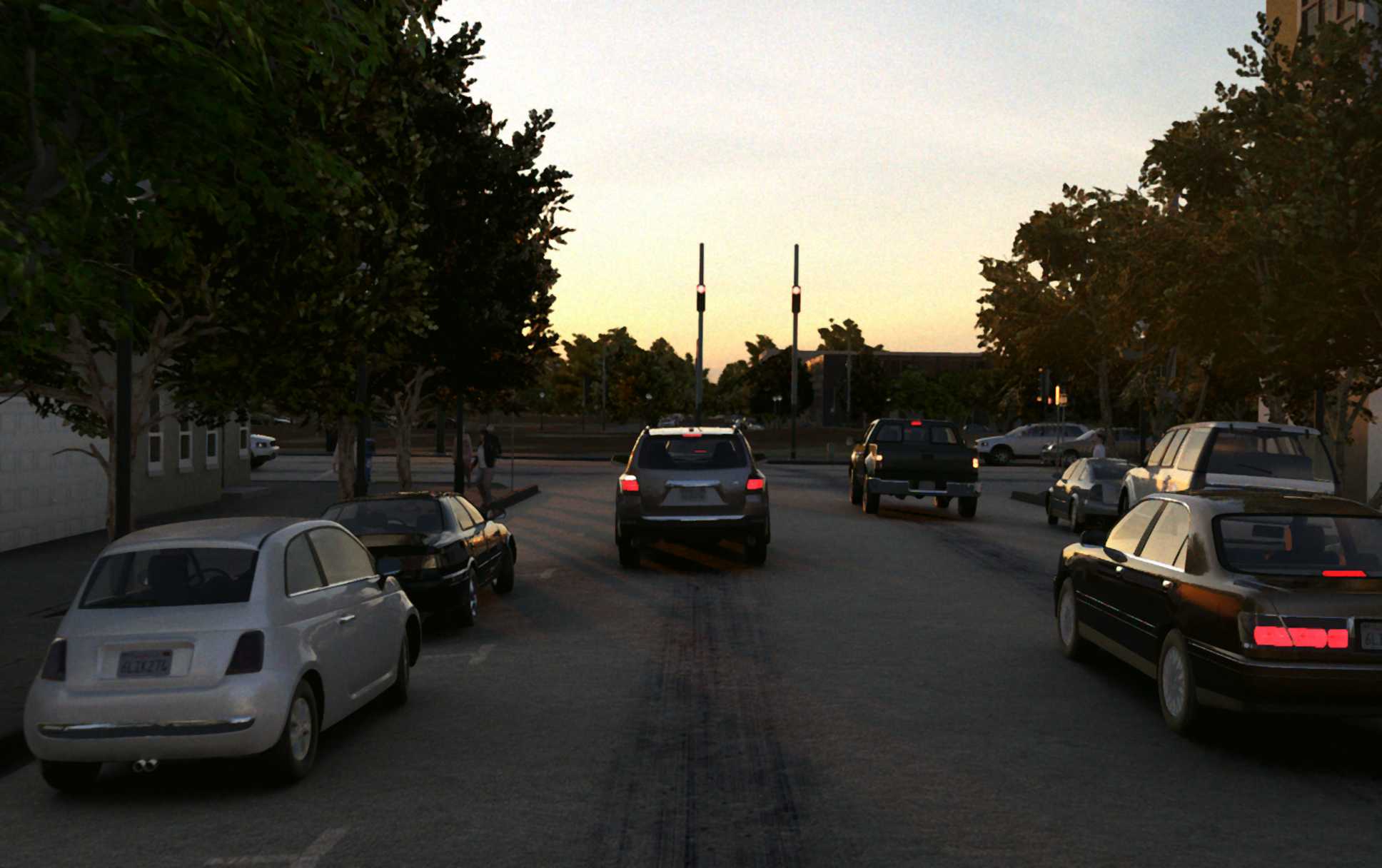
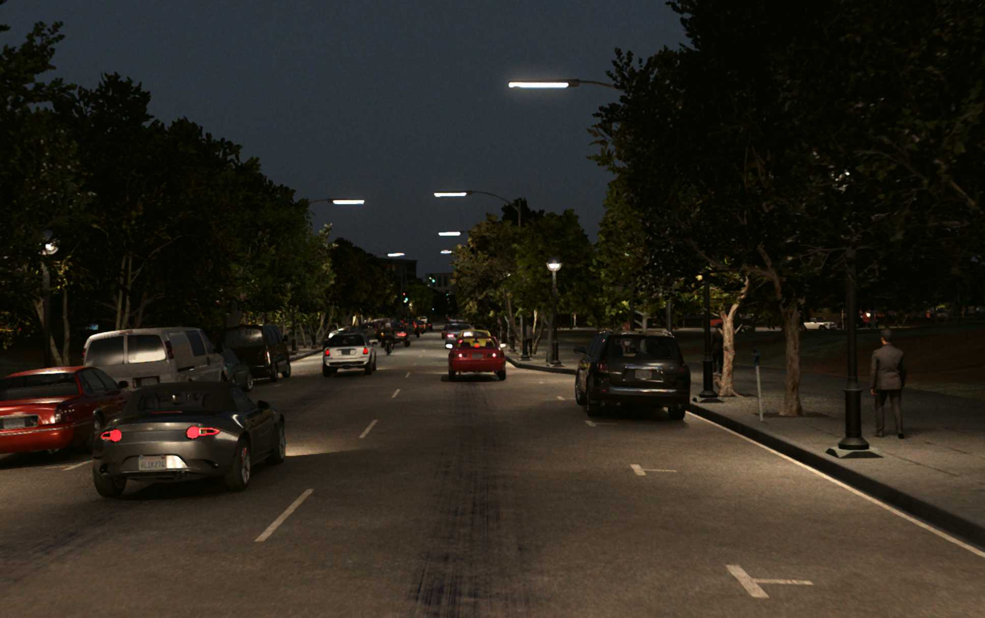
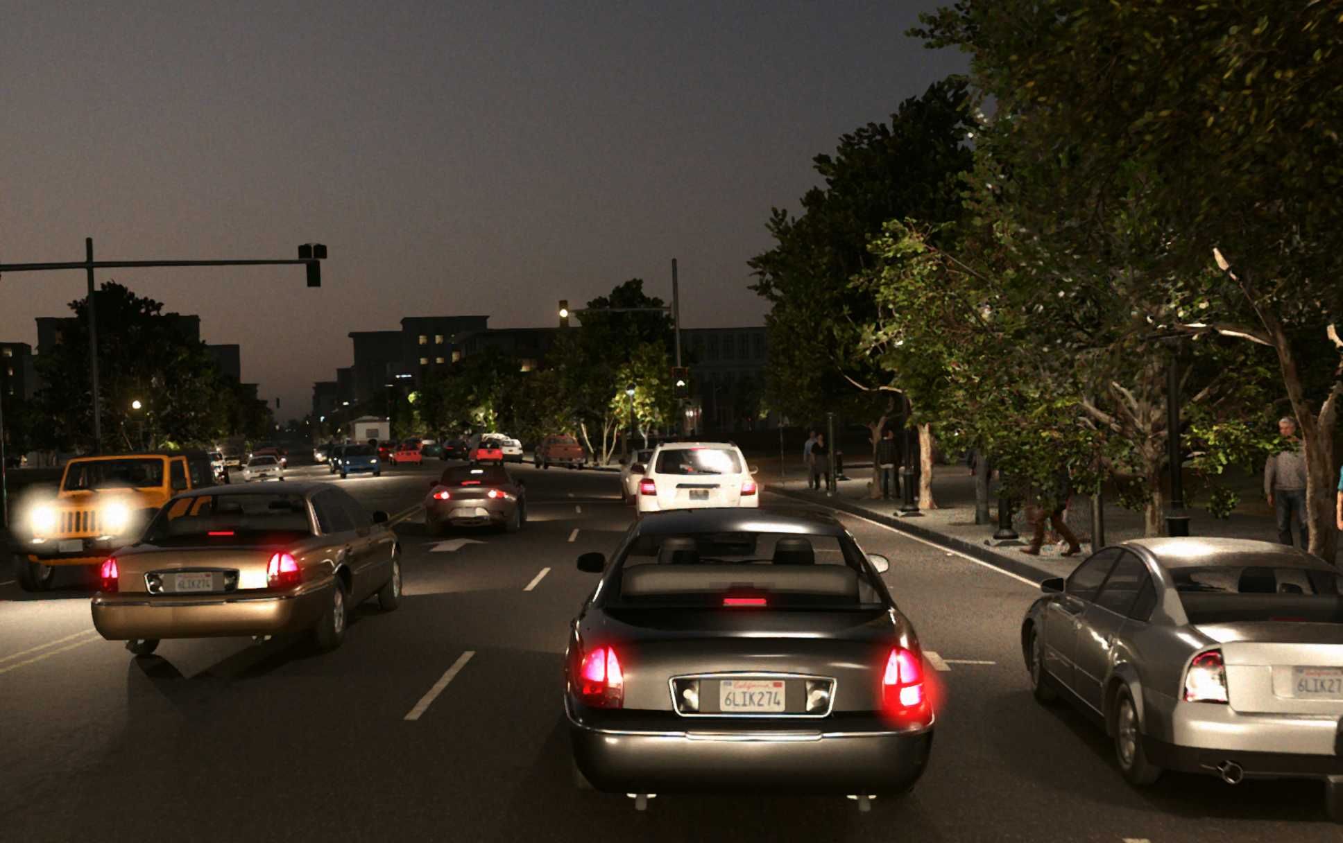
(a)

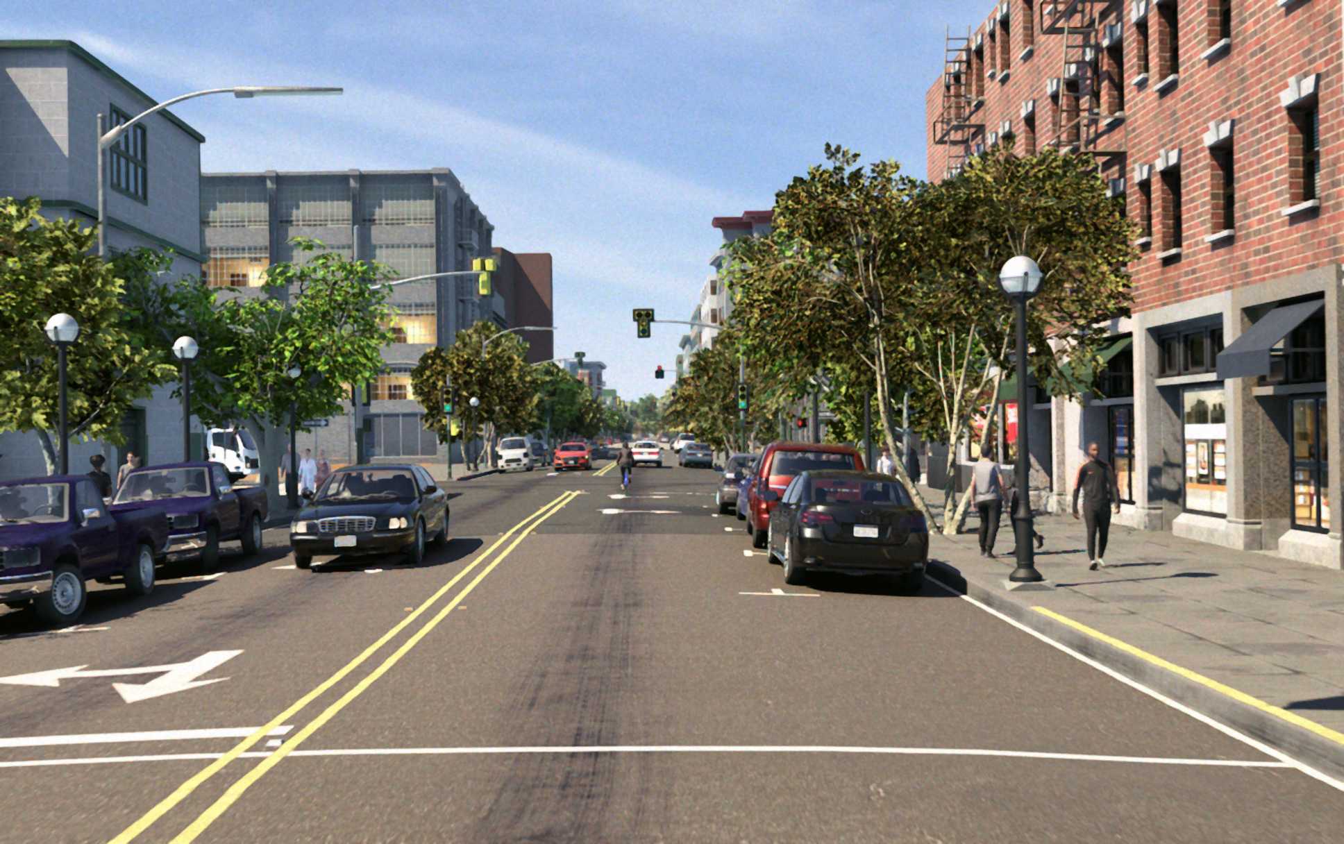
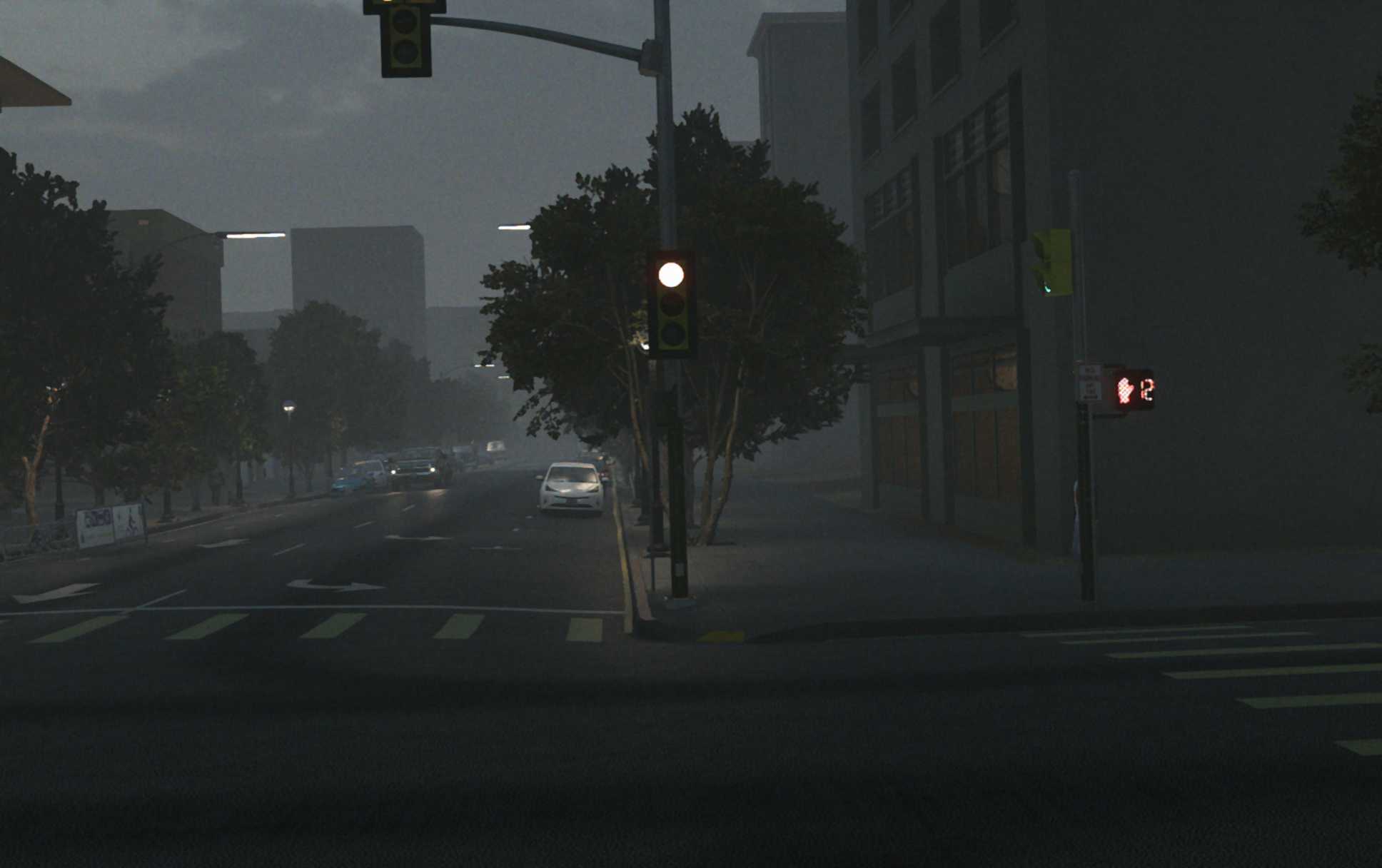
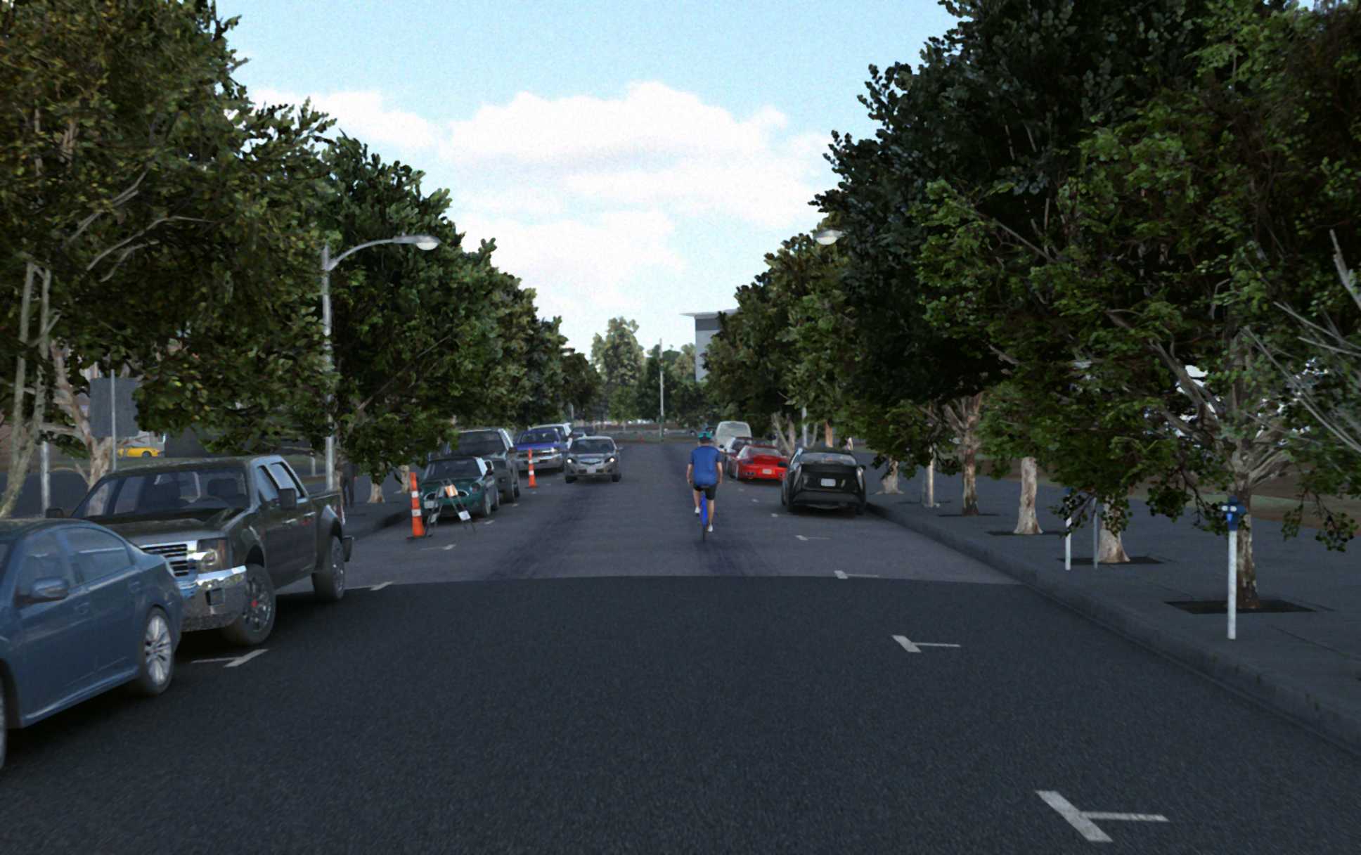
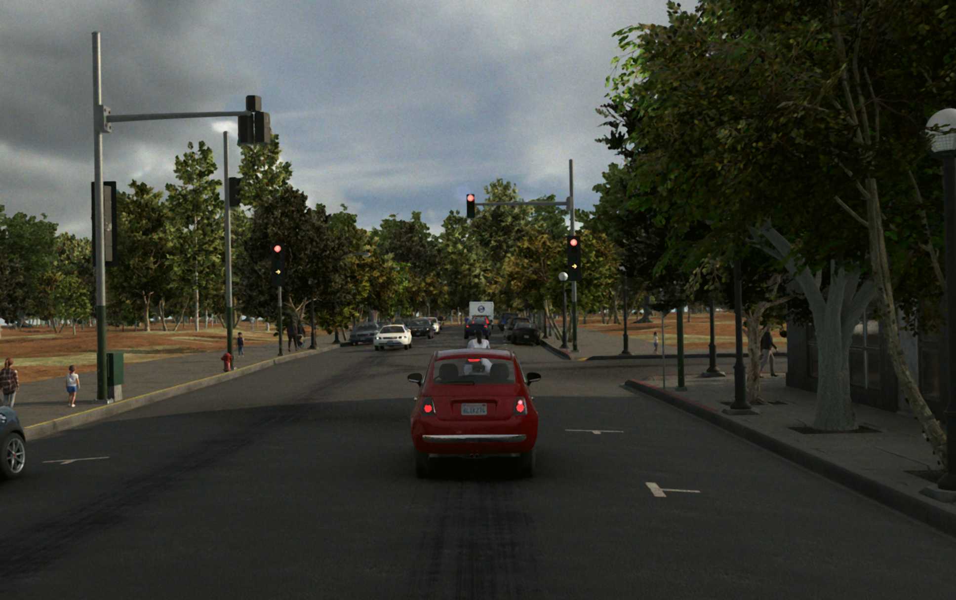
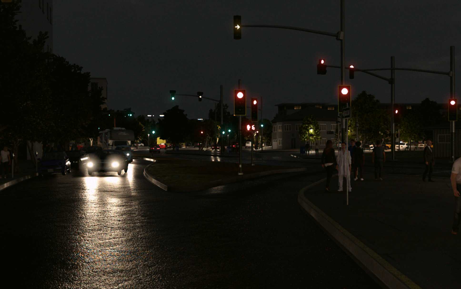
(b)

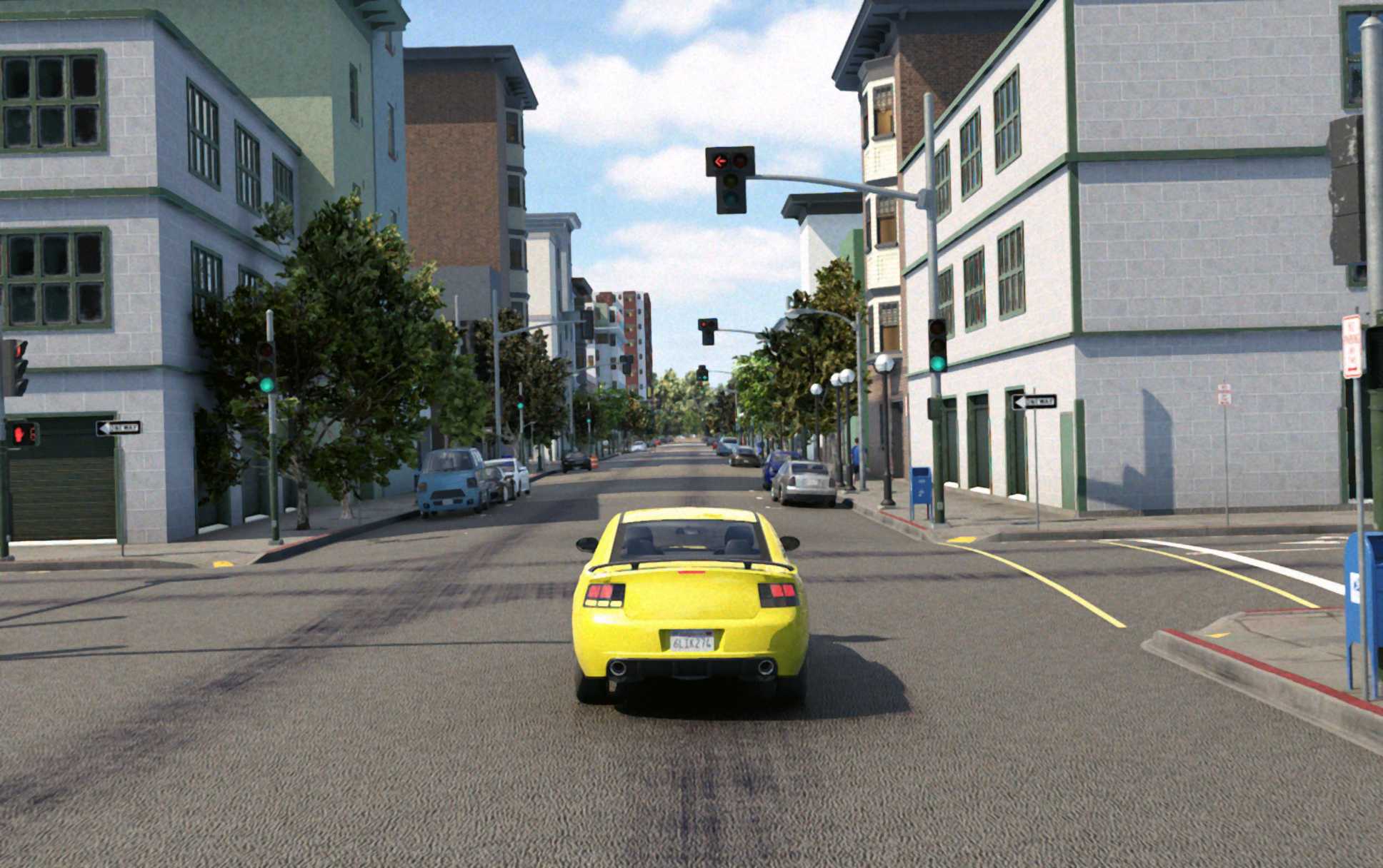
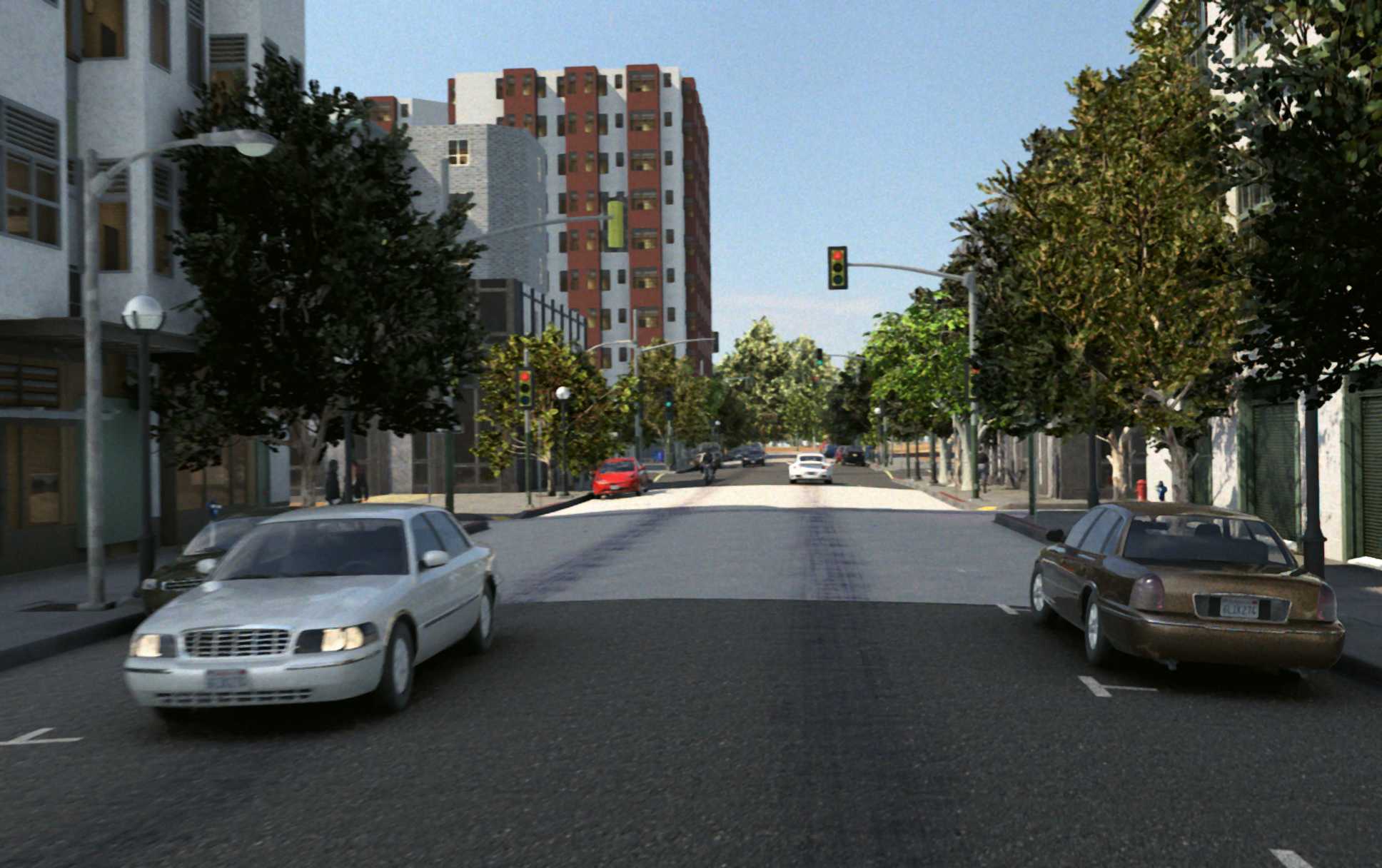
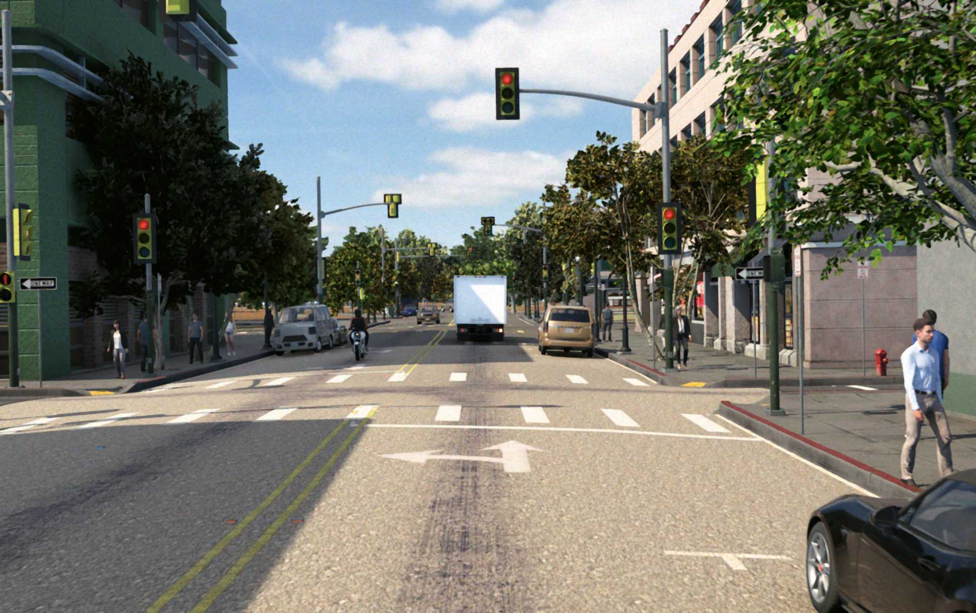
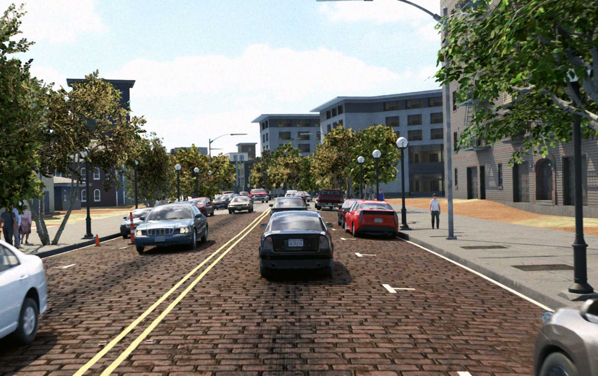
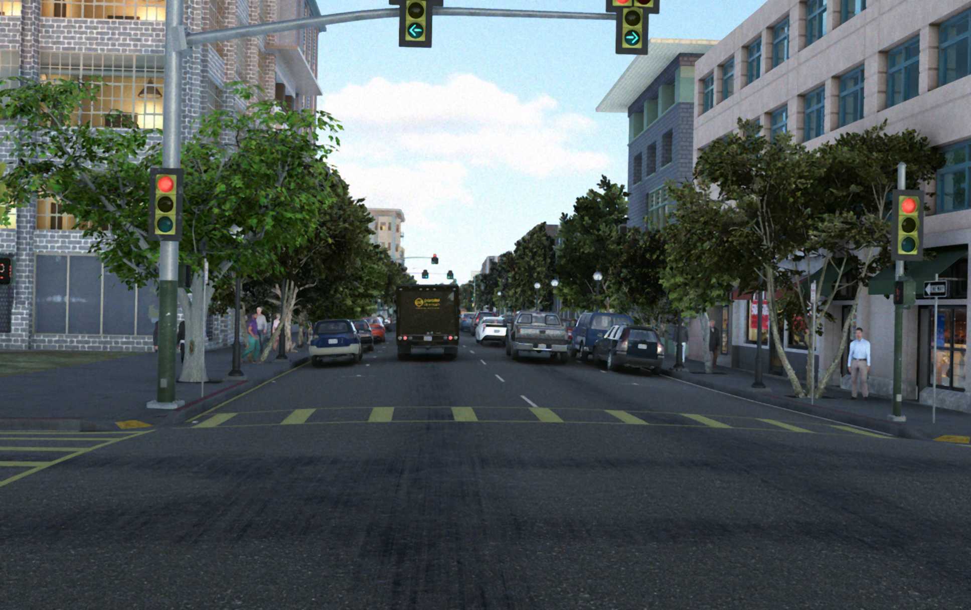
(c)

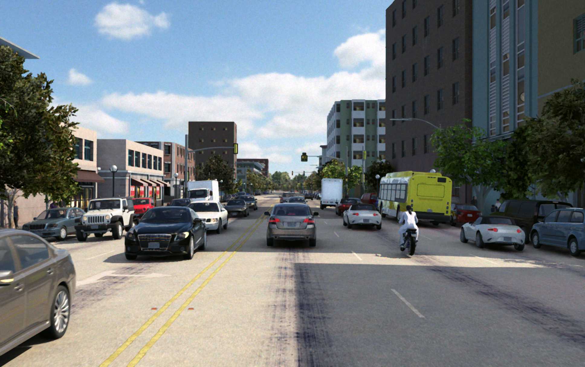
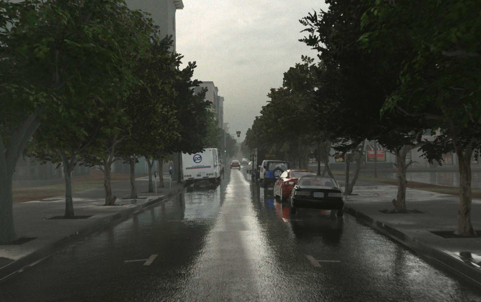
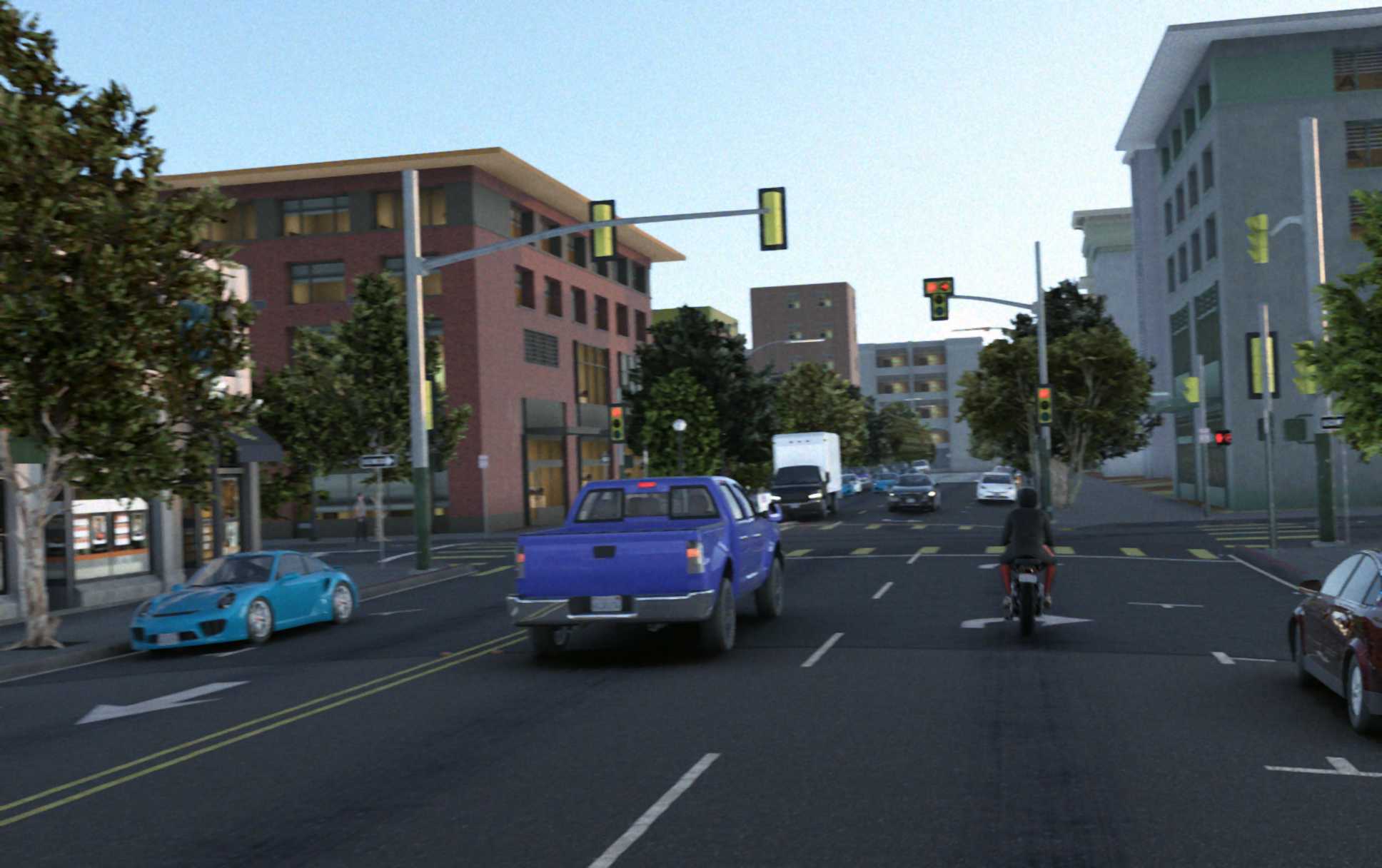
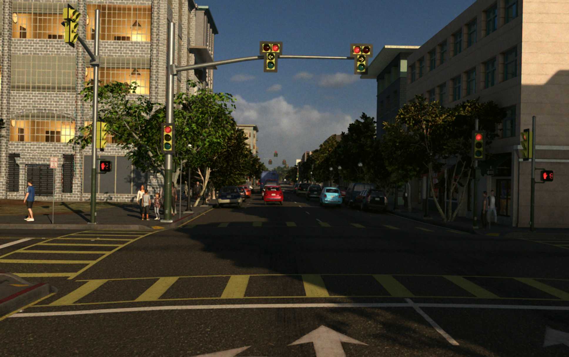
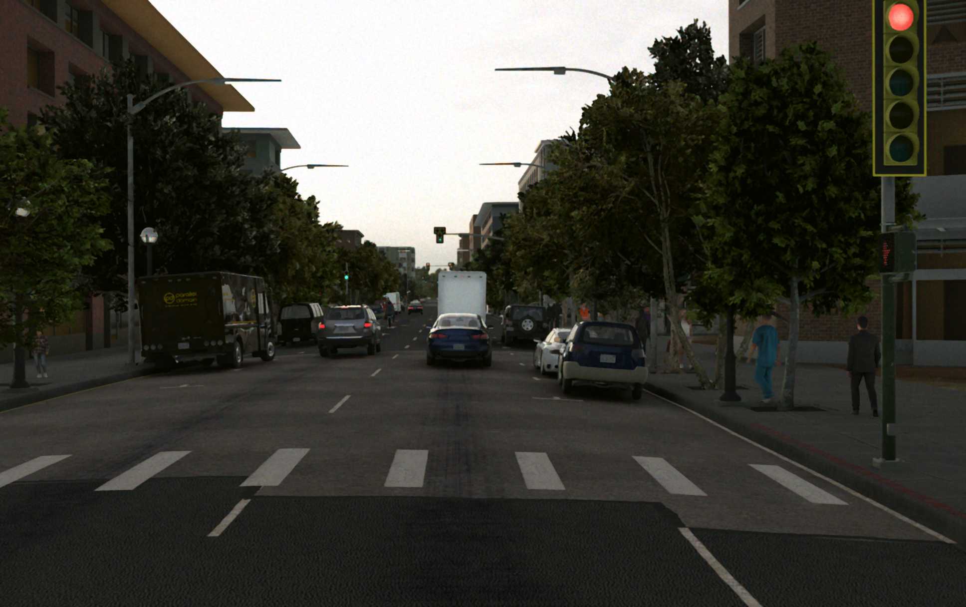
(d)

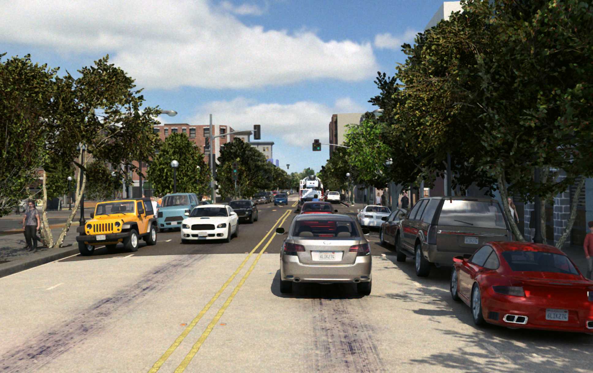
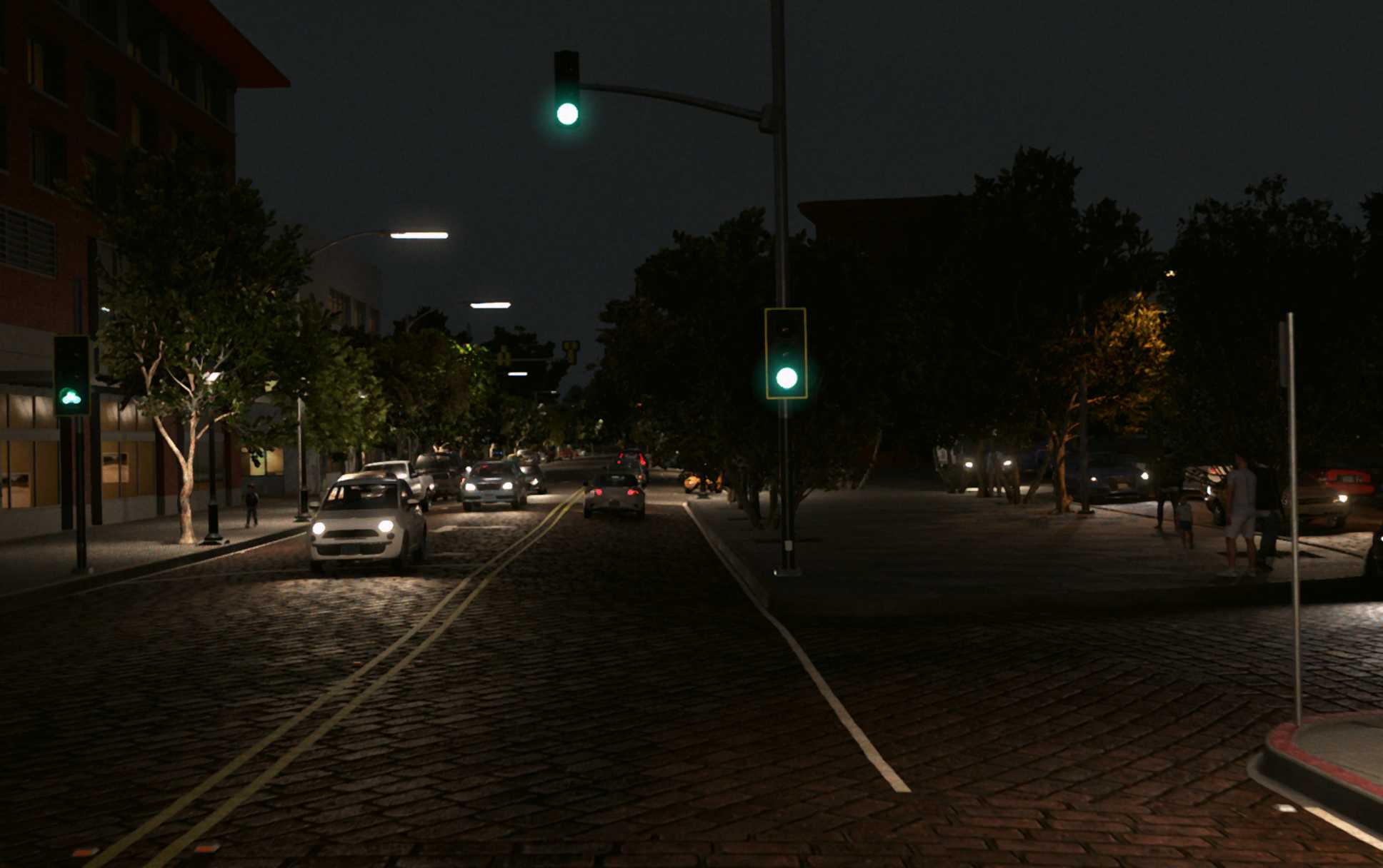
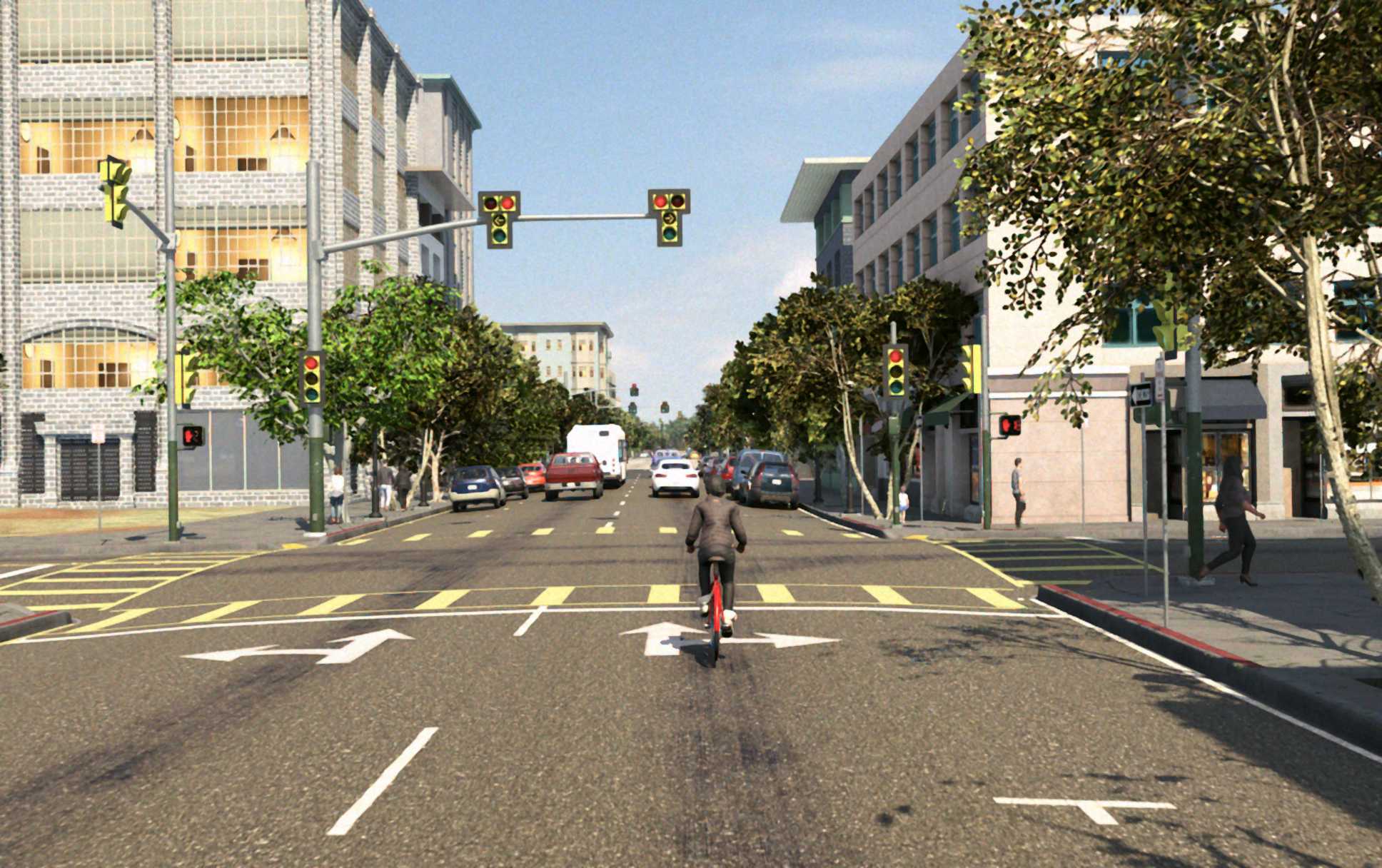
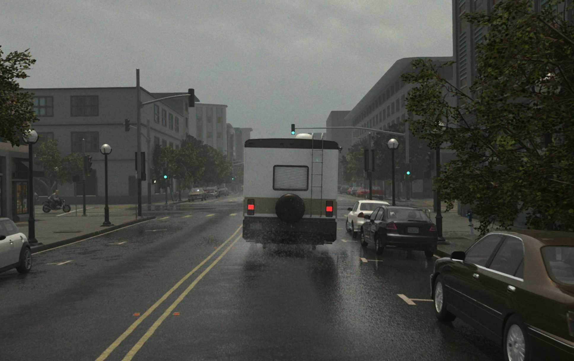
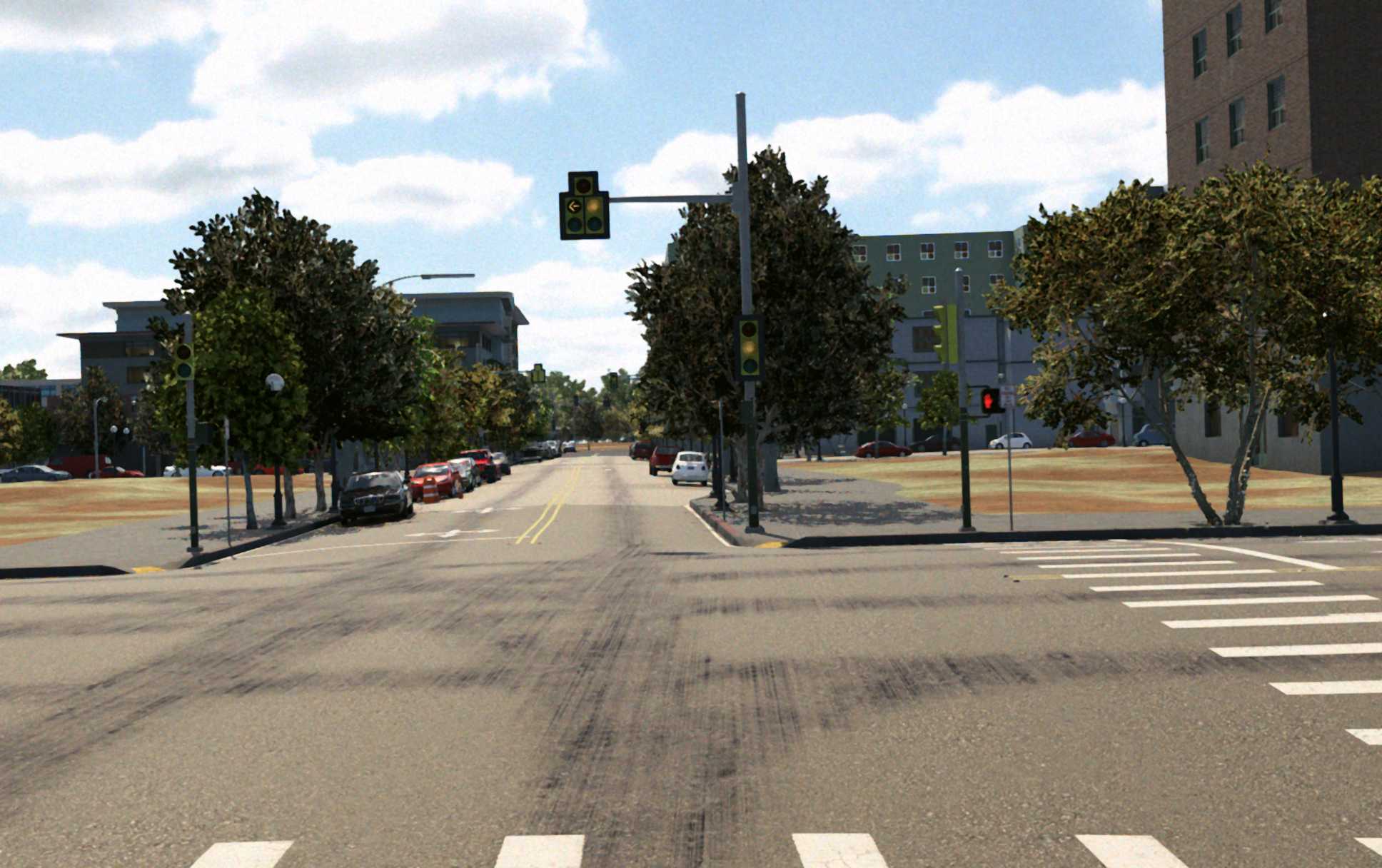
(e)

Figure 10: The Parallel Domain dataset: sample images.

	Layer Description	Out. Dimension
	2 Stacked RGB images	6$\times$H$\times$W
ResNet18 Encoder
#1	Latent Features	256$\times$H/8$\times$W/8
Pose Decoder
#2	Conv2d $\rightarrow$ ReLU	256$\times$H/8$\times$W/8
#3	Conv2d $\rightarrow$ ReLU	256$\times$H/8$\times$W/8
#4	Conv2d $\rightarrow$ ReLU	256$\times$H/8$\times$W/8
#5	Conv2d $\rightarrow$ Global Pooling	6

Table 5: Pose network. Two concatenated RGB images are used as input for a ResNet18 encoder (the first convolutional layer is duplicated to account for that). The output is a 6-dimensional vector estimating the rigid transformation between frames (translation and rotation in Euler angles).

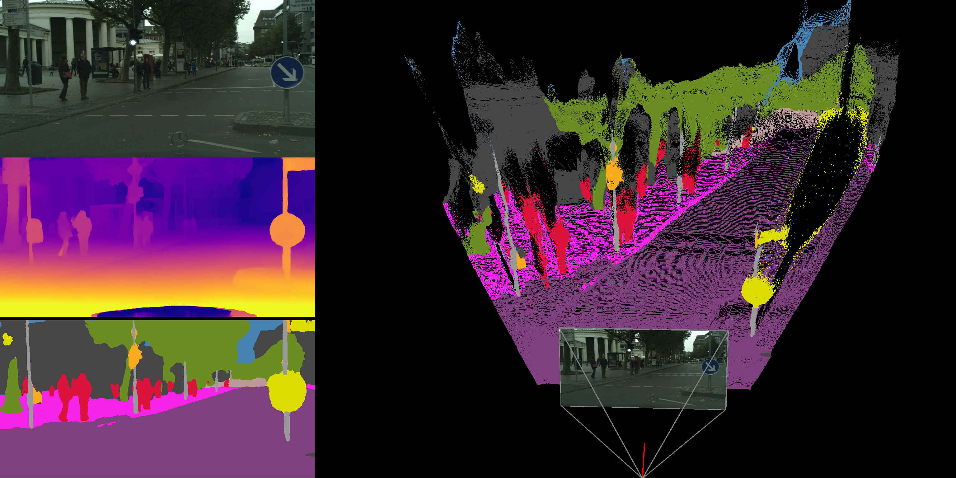
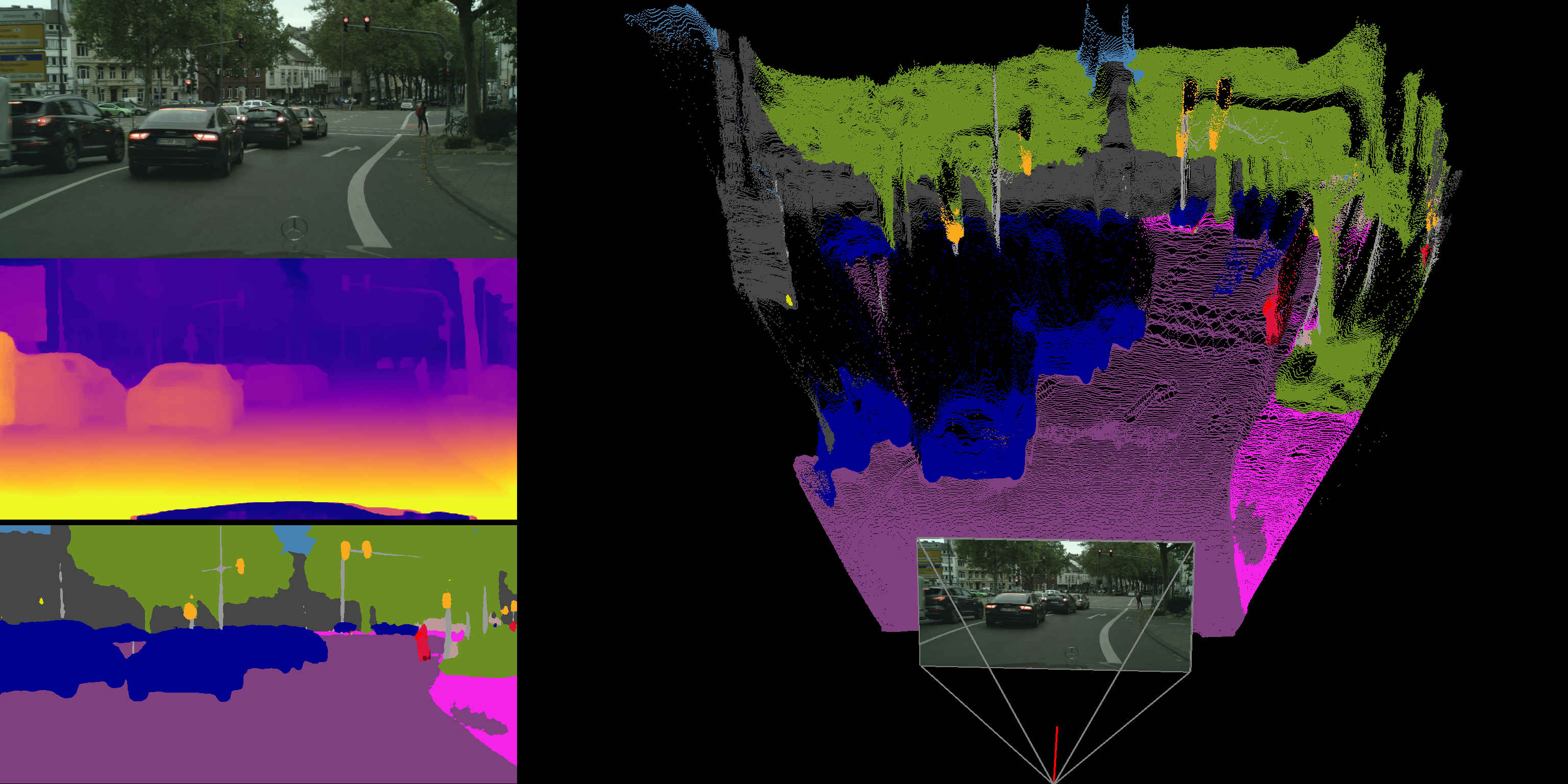
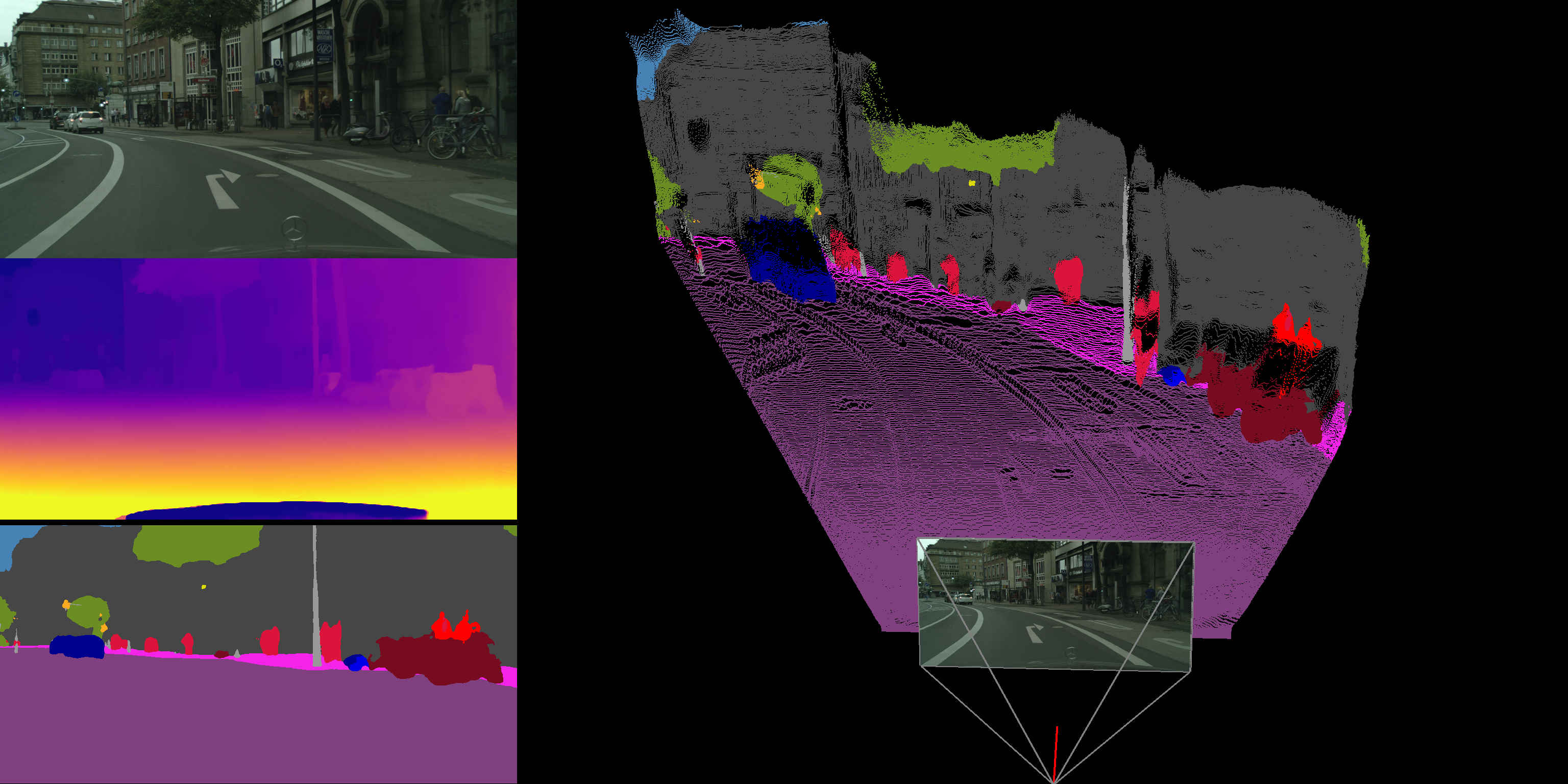
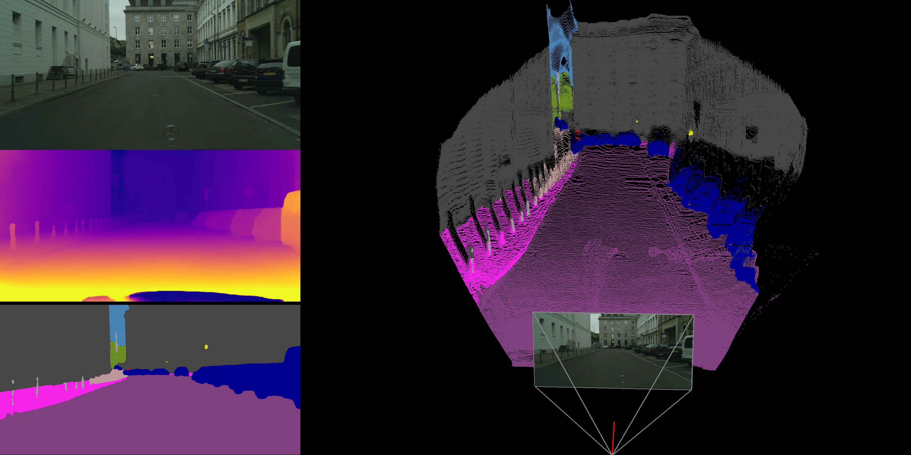
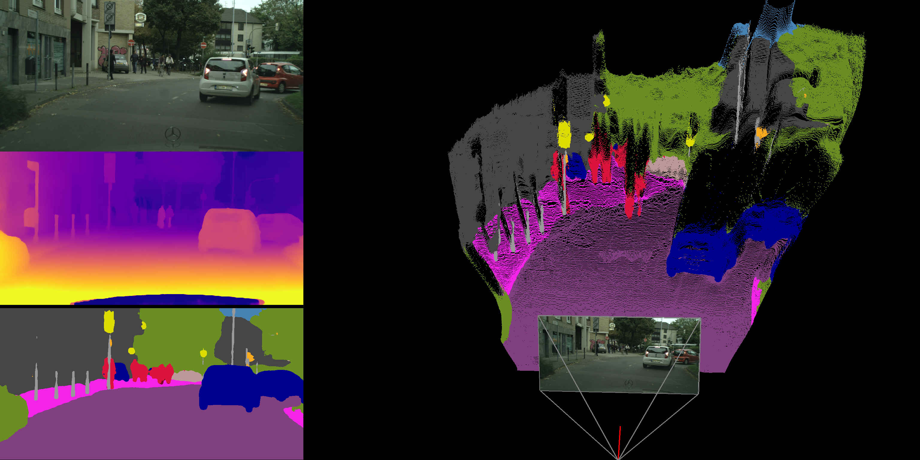
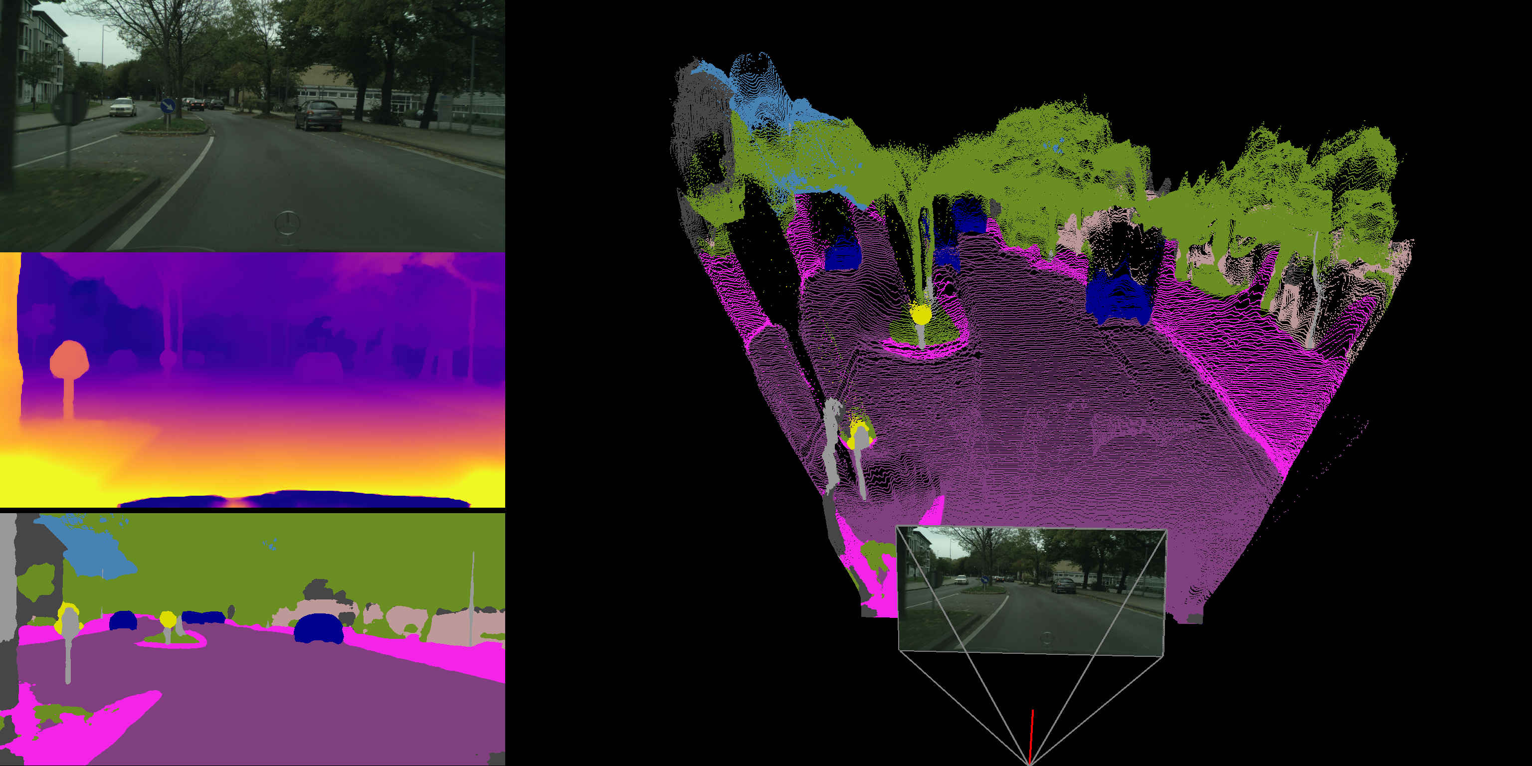
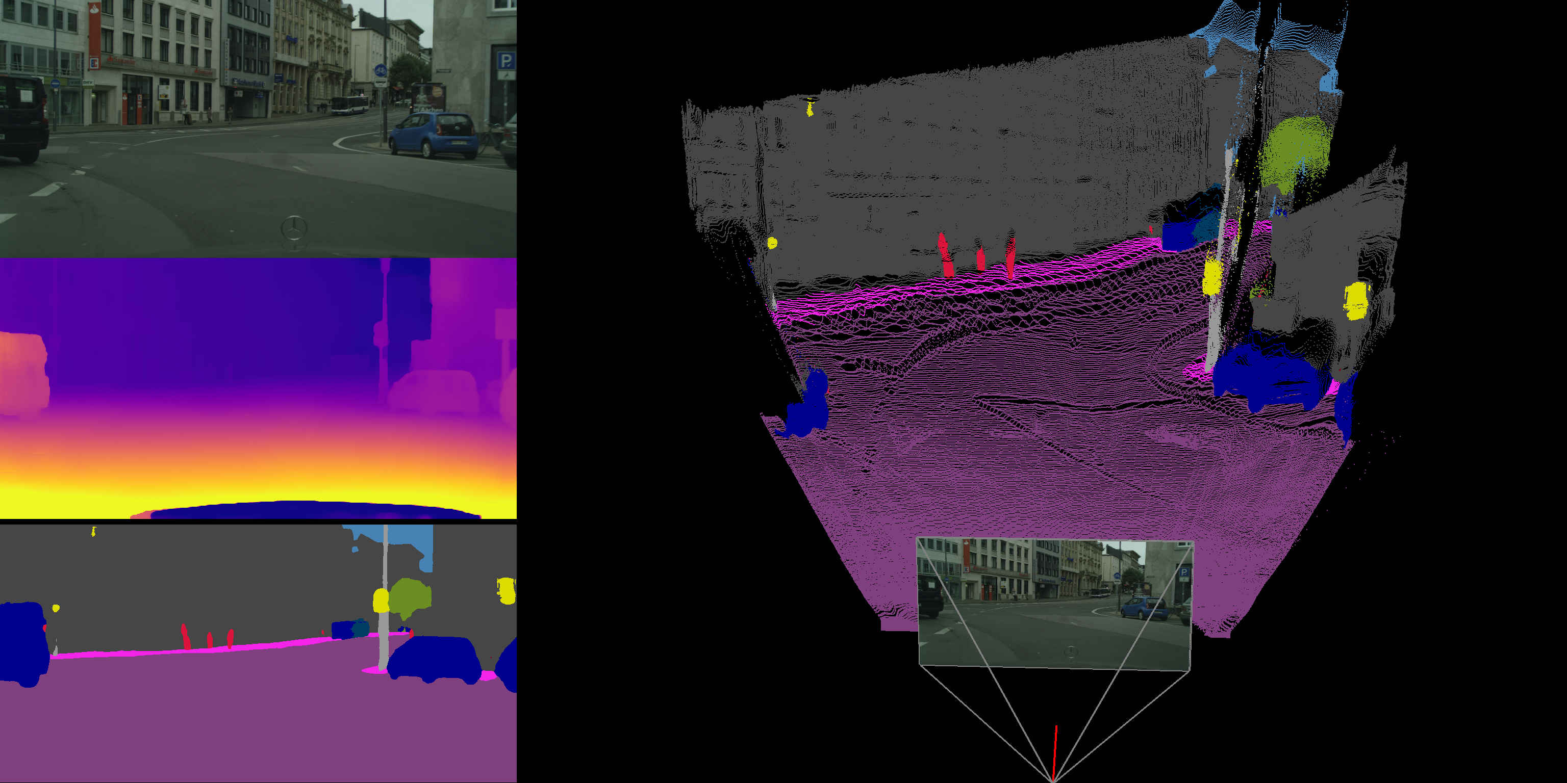
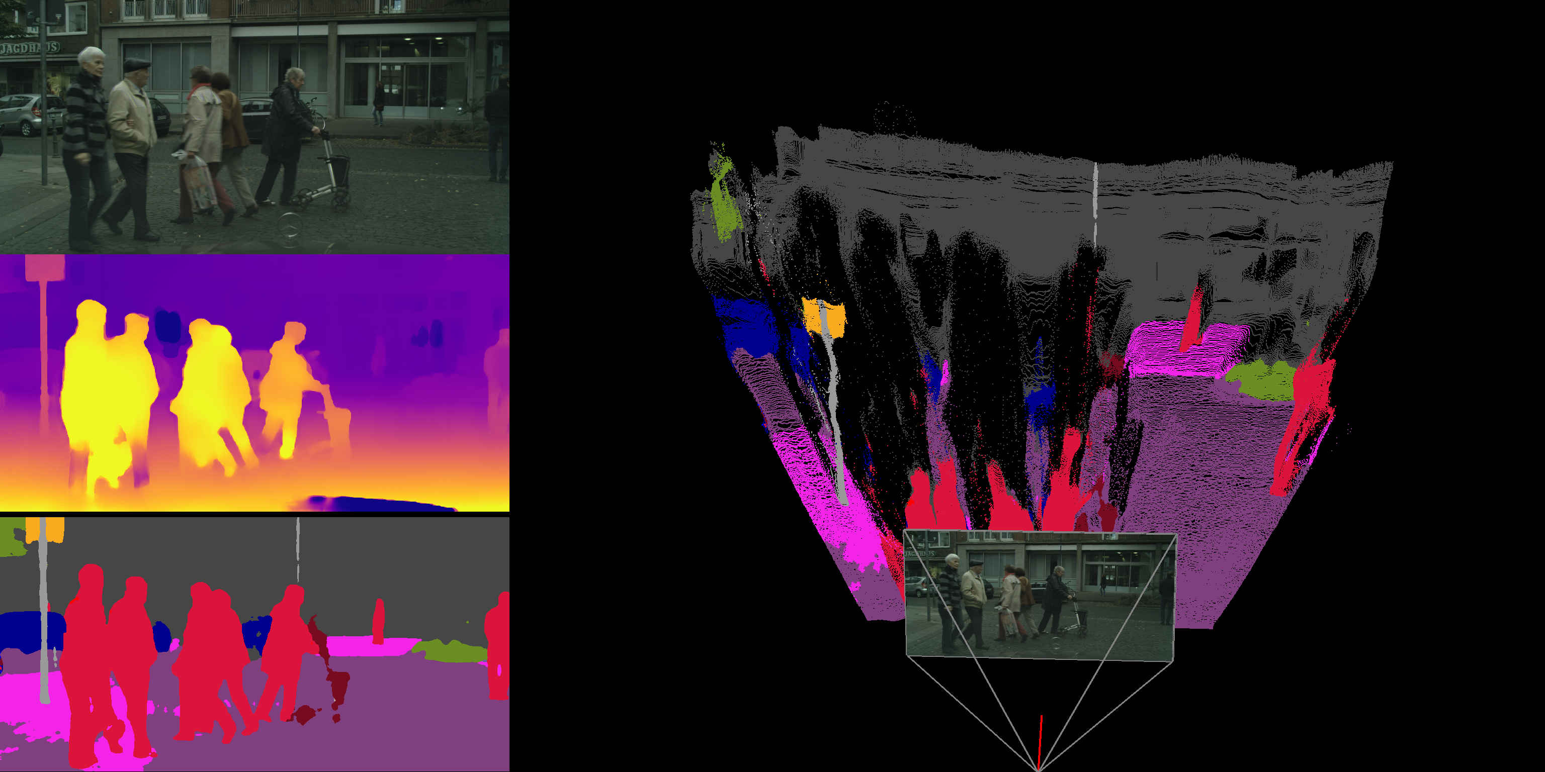
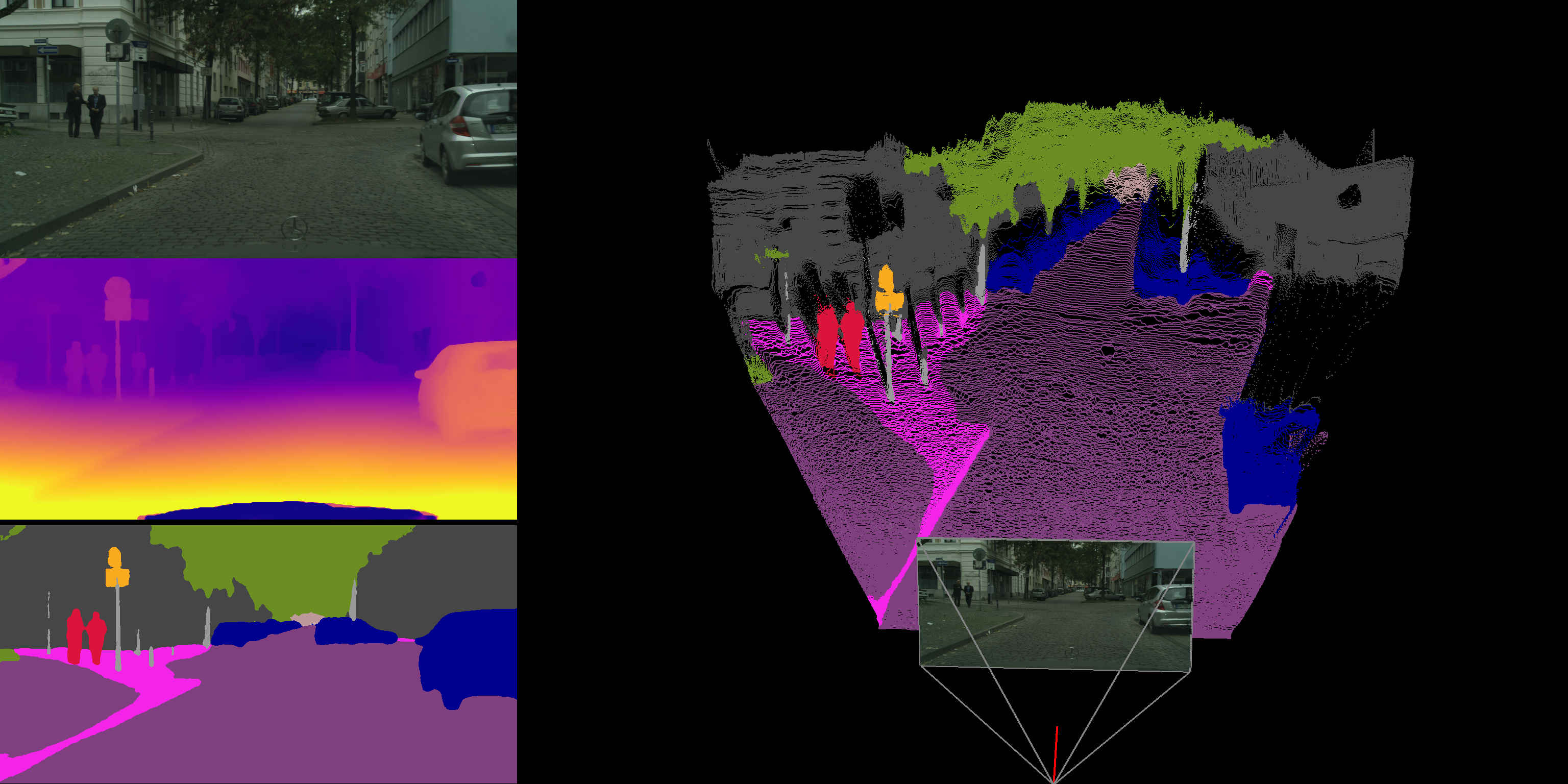
Figure 11: Qualitative depth and semantic segmentation results, using GUDA+PL to perform unsupervised domain adaptation from Parallel Domain to Cityscapes. The same multi-task network was used to generate depth and semantic segmentation estimates, that were combined into a 3D pointcloud using camera intrinsics. No real-world labels (depth or semantic) were used during training.

Our pose network is described in Tab. 5, and follows closely [26]. It uses a ResNet18 backbone as encoder, followed by four convolutional layers with 256 channels. Finally, a global pooling layer outputs a 6-dimensional vector, containing $(x,y,z)$ translation and (roll, pitch, yaw) rotation. We have experimented with a shared encoder for depth, semantic segmentation and pose, however as pointed out in [26] performance degraded in this configuration.

Appendix B Parallel Domain

This dataset is procedurally generated using the Parallel Domain synthetic data generation service [1]. It contains 5000 10-frame sequences, for a total of $50000$ frames. Each frame consists of an RGB image from a front-facing vehicle-mounted camera along with associated per-pixel depth and semantic segmentation labels. The dataset consists of urban and highway environments with varying number of agents, time of day, and weather conditions. We present reference images from the dataset in Fig. 10. Each image is rendered with a $1936\times 1216$ resolution. The high degree of fidelity and perceptual quality allows us to investigate the following questions: (i) how does the quality of the simulation affect the sim-to-real domain gap; and (ii) can we decrease the sim-to-real domain gap with additional synthetic data. As reported in the main paper, Tab. $\color[rgb]{1,0,0}1$ and Fig. $\color[rgb]{1,0,0}7$, we conclude that high quality synthetic data can indeed help narrow the sim-to-real gap, and the gap is further narrowed as additional data is made available.

Method	Road	S.walk	Build.	Wall*	Fence*	Pole*	T.Light	T.Sign	Vegt.	Sky	Person	Rider	Car	Bus	Motor.	Bike	mIoU	mIoU*
Source (SY)	70.2	35.0	74.7	2.1	0.2	27.8	1.7	4.4	76.9	83.4	44.4	9.9	51.3	7.9	4.0	12.8	31.7	36.7
Source (PD)	85.5	39.4	70.6	0.0	0.8	37.6	25.4	11.9	79.9	80.9	47.0	25.0	70.1	10.7	9.8	15.3	38.1	44.0
Target	97.1	82.9	90.6	47.3	51.7	57.1	60.8	72.5	91.6	93.3	75.8	54.3	93.4	77.5	48.5	71.9	72.9	77.8
(a) Comparison with other depth-based UDA methods (SYNTHIA $\rightarrow$ Cityscapes)
SPIGAN [39]	71.1	29.8	71.4	3.7	0.3	33.2	6.4	15.6	81.2	78.9	52.7	13.1	75.9	25.5	10.0	20.5	36.8	42.4
GIO-Ada [8]	78.3	29.2	76.9	11.4	0.3	26.5	10.8	17.2	81.7	81.9	45.8	15.4	68.0	15.9	7.5	30.4	37.3	43.0
DADA [66]	89.2	44.8	81.4	6.8	0.3	26.2	8.6	11.1	81.8	84.0	54.7	19.3	79.7	40.7	14.0	38.8	42.6	49.8
GUDA	85.4	49.5	80.8	13.8	0.9	36.2	21.8	35.2	78.8	84.7	59.9	13.5	84.0	33.8	2.8	30.9	44.5	50.9
(b) Comparison with other UDA methods (SYNTHIA $\rightarrow$ Cityscapes)
Xu et al. [72]	—	—	—	—	—	—	—	—	—	—	—	—	—	—	—	—	38.8	—
CLAN [42]	81.3	37.0	80.1	—	—	—	16.1	13.7	78.2	81.5	53.4	21.2	73.0	32.9	22.6	30.7	—	47.8
CBST [83]	53.6	23.7	75.0	12.5	0.3	36.4	23.5	26.3	84.8	74.7	67.2	17.5	84.5	28.4	15.2	55.8	42.5	48.4
CRST [82]	67.7	32.2	73.9	10.7	1.6	37.4	22.2	31.2	80.8	80.5	60.8	29.1	82.8	25.0	19.4	45.3	43.8	50.1
ESL[55]	84.3	39.7	79.0	9.4	0.7	27.7	16.0	14.3	78.3	83.8	59.1	26.6	72.7	35.8	23.6	45.8	43.5	50.7
FDA [75]	79.3	35.0	73.2	—	—	—	19.9	24.0	61.7	82.6	61.4	31.1	83.9	40.8	38.4	51.1	—	52.5
CCMD [40]	79.6	36.4	80.6	13.3	0.3	25.5	22.4	14.9	81.8	77.4	56.8	25.9	80.7	45.3	29.9	52.0	45.2	52.6
Yang et al. [74]	85.1	44.5	81.0	—	—	—	16.4	15.2	80.1	84.8	59.4	31.9	73.2	41.0	32.6	44.7	53.1
USAMR [78]	83.1	38.2	81.7	9.3	1.0	35.1	30.3	19.9	82.0	80.1	62.8	21.1	84.4	37.8	24.5	53.3	46.5	53.8
IAST [36]	81.9	41.5	83.3	17.7	4.6	32.3	30.9	28.8	83.4	85.0	65.5	30.8	86.5	38.2	33.1	52.7	49.8	57.0
GUDA+PL	88.1	53.0	84.0	22.0	1.4	39.6	28.2	24.8	82.7	81.5	65.5	22.7	89.3	50.5	25.1	57.5	51.0	57.9
(c) Comparison with the state of the art (Varying Sources $\rightarrow$ Cityscapes)
UDAS [58]	86.6	37.8	80.8	29.7	16.4	28.9	30.9	22.2	37.1	76.9	60.1	7.8	84.1	32.1	23.2	13.3	44.3	49.2
USAMR (G5) [78]	90.5	35.0	84.6	34.3	24.0	36.8	44.1	42.7	84.5	82.5	63.1	34.4	85.8	38.2	27.1	41.8	53.1	58.0
IAST (G5) [36]	94.1	58.8	85.4	39.7	29.2	25.1	43.1	34.2	84.8	88.7	62.7	30.3	87.6	50.3	35.2	40.2	55.6	61.2
GUDA(PD)+PL(G5)	92.9	50.5	86.0	17.9	24.0	45.4	50.9	44.5	87.7	87.0	66.6	36.9	89.5	52.1	28.5	54.0	57.2	63.2

Table 6: Semantic segmentation results on Cityscapes using different unsupervised domain adaptation (UDA) methods and synthetic datasets. The mIoU metric considers all 16 classes, and mIoU* considers only the 13 classes present in SYNTHIA (removing the ones marked with *). Source shows results without any adaptation, and Target shows results with semantic supervision on the target domain. Synthetic datasets include: SYNTHIA (SY), Parallel Domain (PD), and GTA5 (G5).

Method	Road	Building	Pole	T. Light	T. Sign	Vegetat.	Terrain	Sky	Car	Truck	mIoU
Source	64.9	28.3	37.8	18.8	11.7	63.7	21.6	78.7	55.3	1.5	38.6
DANN	70.3	49.4	39.5	28.0	22.2	67.0	23.1	82.0	69.4	5.1	45.6
GUDA	86.8	72.7	46.2	41.4	44.6	77.3	29.1	88.5	86.1	9.8	58.25

Table 7: Semantic segmentation results on VKITTI2 $\rightarrow$ KITTI, using GUDA and DANN [18].

Method	Road	S.walk	Build.	Pole	T.Light	T.Sign	Vegetat.	Sky	Person	Rider	Car	Truck	Bus	Motor.	Bike	mIoU
Source	93.9	30.7	49.3	35.7	50.7	20.8	87.2	89.3	10.0	28.7	63.2	38.4	14.3	8.5	7.3	41.9
DANN	95.3	36.1	53.0	35.6	52.8	20.7	88.3	90.3	15.2	38.7	67.5	44.1	36.5	19.5	11.1	47.0
GUDA	96.1	48.0	58.9	37.1	55.8	22.0	89.6	93.0	30.6	54.8	70.8	47.2	58.7	41.6	29.6	55.6

Table 8: Semantic segmentation results on Parallel Domain $\rightarrow$ DDAD, using GUDA and DANN [18].

Appendix C Qualitative Results

In Fig. 11 we present semantic pointclouds estimated using GUDA+PL for unsupervised domain adaptation from Parallel Domain to Cityscapes. Because our multi-task network (Tab. 4) produces both depth and semantic segmentation estimates, we can lift the predicted semantic labels to 3D space using depth estimates and camera intrinsics. Each pixel is assigned a 3D coordinate in the camera frame of reference, as well as RGB colors and semantic logits. We emphasize that no real-world labels (depth maps or semantic classes) were used at any point during the training of this network, only image sequences. All labeled information was obtained from synthetic datasets, and adapted to better align with real-world data using our proposed GUDA approach to geometric unsupervised domain adaptation.

Appendix D Detailed Tables

We also present detailed tables to complement some results from the main paper. In particular, Table 6 expands Table 1 from the main paper, showing per-class results on the Cityscapes dataset of the various methods we use as comparison to validate the improvements of our proposed GUDA approach. Similarly, Tables 7 and 8 expand Figures 5 and 6 from the main paper, showing respectively GUDA results from our VKITTI2 to KITTI and PD to DDAD experiments relative to source-only and DANN [18].

References

- [1] Parallel domain. https://paralleldomain.com/, March 2021.
- [2] Hassan Alhaija, Siva Mustikovela, Lars Mescheder, Andreas Geiger, and Carsten Rother. Augmented reality meets computer vision: Efficient data generation for urban driving scenes. International Journal of Computer Vision (IJCV), 2018.
- [3] Konstantinos Bousmalis, Nathan Silberman, David Dohan, Dumitru Erhan, and Dilip Krishnan. Unsupervised pixel-level domain adaptation with generative adversarial networks. In CVPR, 2017.
- [4] Yohann Cabon, Naila Murray, and Martin Humenberger. Virtual kitti 2, 2020.
- [5] Fabio M Carlucci, Antonio D’Innocente, Silvia Bucci, Barbara Caputo, and Tatiana Tommasi. Domain generalization by solving jigsaw puzzles. In Proceedings of the IEEE Conference on Computer Vision and Pattern Recognition, pages 2229–2238, 2019.
- [6] Liang-Chieh Chen, George Papandreou, Iasonas Kokkinos, Kevin Murphy, and Alan L. Yuille. Deeplab: Semantic image segmentation with deep convolutional nets, atrous convolution, and fully connected crfs. CoRR, 2016.
- [7] Liang-Chieh Chen, Yi Yang, Jiang Wang, Wei Xu, and Alan L Yuille. Attention to scale: Scale-aware semantic image segmentation. In CVPR, 2016.
- [8] Yuhua Chen, Wen Li, Xiaoran Chen, and Luc Van Gool. Learning semantic segmentation from synthetic data: A geometrically guided input-output adaptation approach. In Proceedings of the IEEE/CVF Conference on Computer Vision and Pattern Recognition (CVPR), June 2019.
- [9] Djork-Arné Clevert, Thomas Unterthiner, and Sepp Hochreiter. Fast and accurate deep network learning by exponential linear units (elus). In ICLR, 2016.
- [10] Marius Cordts, Mohamed Omran, Sebastian Ramos, Timo Rehfeld, Markus Enzweiler, Rodrigo Benenson, Uwe Franke, Stefan Roth, and Bernt Schiele. The cityscapes dataset for semantic urban scene understanding. In IEEE conference on computer vision and pattern recognition, pages 3213–3223, 2016.
- [11] Gabriela Csurka. Domain adaptation for visual applications: A comprehensive survey. arXiv preprint arXiv:1702.05374, 2017.
- [12] César Roberto de Souza, Adrien Gaidon, Yohann Cabon, Naila Murray, and Antonio Manuel López. Generating human action videos by coupling 3d game engines and probabilistic graphical models. IJCV, pages 1–32, 2019.
- [13] Jia Deng, Wei Dong, Richard Socher, Li jia Li, Kai Li, and Li Fei-fei. Imagenet: A large-scale hierarchical image database. In Proceedings of the IEEE Conference on Computer Vision and Pattern Recognition, 2009.
- [14] D. Eigen and R. Fergus. Predicting depth, surface normals and semantic labels with a common multi-scale convolutional architecture. In 2015 IEEE International Conference on Computer Vision (ICCV), pages 2650–2658, 2015.
- [15] David Eigen, Christian Puhrsch, and Rob Fergus. Depth map prediction from a single image using a multi-scale deep network. In Advances in neural information processing systems, pages 2366–2374, 2014.
- [16] John Flynn, Ivan Neulander, James Philbin, and Noah Snavely. Deepstereo: Learning to predict new views from the world’s imagery. In Proceedings of the IEEE Conference on Computer Vision and Pattern Recognition, pages 5515–5524, 2016.
- [17] Adrien Gaidon, Qiao Wang, Yohann Cabon, and Eleonora Vig. Virtual worlds as proxy for multi-object tracking analysis. In Proceedings of the IEEE conference on computer vision and pattern recognition, pages 4340–4349, 2016.
- [18] Yaroslav Ganin, Evgeniya Ustinova, Hana Ajakan, Pascal Germain, Hugo Larochelle, François Laviolette, Mario Marchand, and Victor Lempitsky. Domain-adversarial training of neural networks. JMLR, 17(1):2096–2030, Jan. 2016.
- [19] Ravi Garg, Vijay Kumar BG, Gustavo Carneiro, and Ian Reid. Unsupervised cnn for single view depth estimation: Geometry to the rescue. In European Conference on Computer Vision, pages 740–756. Springer, 2016.
- [20] Andreas Geiger, Philip Lenz, Christoph Stiller, and Raquel Urtasun. Vision meets robotics: The kitti dataset. The International Journal of Robotics Research, 32(11):1231–1237, 2013.
- [21] Andreas Geiger, Philip Lenz, and Raquel Urtasun. Are we ready for autonomous driving? the kitti vision benchmark suite. In Conference on Computer Vision and Pattern Recognition (CVPR), 2012.
- [22] Muhammad Ghifary, W Bastiaan Kleijn, Mengjie Zhang, David Balduzzi, and Wen Li. Deep reconstruction-classification networks for unsupervised domain adaptation. In European Conference on Computer Vision, pages 597–613. Springer, 2016.
- [23] Spyros Gidaris, Praveer Singh, and Nikos Komodakis. Unsupervised representation learning by predicting image rotations. arXiv preprint arXiv:1803.07728, 2018.
- [24] Clément Godard, Oisin Mac Aodha, and Gabriel J Brostow. Unsupervised monocular depth estimation with left-right consistency. In CVPR, volume 2, page 7, 2017.
- [25] Clément Godard, Oisin Mac Aodha, and Gabriel J. Brostow. Unsupervised monocular depth estimation with left-right consistency. In CVPR, 2017.
- [26] Clément Godard, Oisin Mac Aodha, Michael Firman, and Gabriel J. Brostow. Digging into self-supervised monocular depth prediction. In ICCV, 2019.
- [27] Ariel Gordon, Hanhan Li, Rico Jonschkowski, and Anelia Angelova. Depth from videos in the wild: Unsupervised monocular depth learning from unknown cameras. In Proceedings of the IEEE International Conference on Computer Vision, pages 8977–8986, 2019.
- [28] Vitor Guizilini, Rares Ambrus, Sudeep Pillai, Allan Raventos, and Adrien Gaidon. 3d packing for self-supervised monocular depth estimation. In International Conference on Computer Vision and Pattern Recognition (CVPR), 2020.
- [29] Vitor Guizilini, Rui Hou, Jie Li, Rares Ambrus, and Adrien Gaidon. Semantically-guided representation learning for self-supervised monocular depth. arXiv preprint arXiv:2002.12319, 2020.
- [30] Kaiming He, Xiangyu Zhang, Shaoqing Ren, and Jian Sun. Deep residual learning for image recognition. In Proceedings of the IEEE conference on computer vision and pattern recognition, pages 770–778, 2016.
- [31] Judy Hoffman, Eric Tzeng, Taesung Park, Jun-Yan Zhu, Phillip Isola, Kate Saenko, Alexei Efros, and Trevor Darrell. Cycada: Cycle-consistent adversarial domain adaptation. In International conference on machine learning, pages 1989–1998. PMLR, 2018.
- [32] Judy Hoffman, Dequan Wang, Fisher Yu, and Trevor Darrell. Fcns in the wild: Pixel-level adversarial and constraint-based adaptation. arXiv preprint arXiv:1612.02649, 2016.
- [33] Haoshuo Huang, Qixing Huang, and Philipp Krahenbuhl. Domain transfer through deep activation matching. In Proceedings of the European Conference on Computer Vision (ECCV), pages 590–605, 2018.
- [34] Junhwa Hur and Stefan Roth. Self-supervised monocular scene flow estimation. In CVPR, 2020.
- [35] SouYoung Jin, Aruni RoyChowdhury, Huaizu Jiang, Ashish Singh, Aditya Prasad, Deep Chakraborty, and Erik Learned-Miller. Unsupervised hard example mining from videos for improved object detection. In European Conference on Computer Vision (ECCV), 2018.
- [36] Jiaqi Zou Ke Mei, Chuang Zhu and Shanghang Zhang. Instance adaptive self-training for unsupervised domain adaptation. In European Conference on Computer Vision (ECCV), 2020.
- [37] Gustav Larsson, Michael Maire, and Gregory Shakhnarovich. Learning representations for automatic colorization. In European conference on computer vision, pages 577–593. Springer, 2016.
- [38] Jin Han Lee, Myung-Kyu Han, Dong Wook Ko, and Il Hong Suh. From big to small: Multi-scale local planar guidance for monocular depth estimation. arXiv preprint arXiv:1907.10326, 2019.
- [39] Kuan-Hui Lee, German Ros, Jie Li, and Adrien Gaidon. SPIGAN: privileged adversarial learning from simulation. In 7th International Conference on Learning Representations, ICLR 2019, New Orleans, LA, USA, May 6-9, 2019, 2019.
- [40] Guangrui Li, Guoliang Kang, Wu Liu, Yunchao Wei, and Yi Yang. Content-consistent matching for domain adaptive semantic segmentation. In European Conference on Computer Vision (ECCV), 2020.
- [41] Ilya Loshchilov and Frank Hutter. Decoupled weight decay regularization. In International Conference on Learning Representations, 2019.
- [42] Yawei Luo, Liang Zheng, Tao Guan, Junqing Yu, and Yi Yang. Taking a closer look at domain shift: Category-level adversaries for semantics consistent domain adaptation. In The IEEE Conference on Computer Vision and Pattern Recognition (CVPR), 2019.
- [43] I. Misra, A. Shrivastava, A. Gupta, and M. Hebert. Cross-stitch networks for multi-task learning. In 2016 IEEE Conference on Computer Vision and Pattern Recognition (CVPR), pages 3994–4003, 2016.
- [44] Mehdi Noroozi and Paolo Favaro. Unsupervised learning of visual representations by solving jigsaw puzzles. In European Conference on Computer Vision, pages 69–84. Springer, 2016.
- [45] George Papandreou, Liang-Chieh Chen, Kevin Murphy, and Alan L Yuille. Weakly- and semi-supervised learning of a dcnn for semantic image segmentation. In ICCV, 2015.
- [46] Adam Paszke, Sam Gross, Soumith Chintala, Gregory Chanan, Edward Yang, Zachary DeVito, Zeming Lin, Alban Desmaison, Luca Antiga, and Adam Lerer. Automatic differentiation in pytorch. In NIPS-W, 2017.
- [47] Xingchao Peng, Baochen Sun, Karim Ali, and Kate Saenko. Learning deep object detectors from 3d models. In Proceedings of the 2015 IEEE International Conference on Computer Vision (ICCV), ICCV ’15, page 1278–1286, 2015.
- [48] Tobias Pohlen, Alexander Hermans, Markus Mathias, and Bastian Leibe. Full-resolution residual networks for semantic segmentation in street scenes. In Proceedings of the IEEE Conference on Computer Vision and Pattern Recognition, pages 4151–4160, 2017.
- [49] A. Ranja, V. Jampani, K. Kim, D. Sun, J. Wulff, and M. Black. Adversarial collaboration: Joint unsupervised learning of depth, camera motion, optical flow and motion segmentation. arXiv preprint arXiv:1805.09806, 2018.
- [50] Stephan R. Richter, Vibhav Vineet, Stefan Roth, and Vladlen Koltun. Playing for data: Ground truth from computer games. In European Conference on Computer Vision (ECCV), volume 9906 of LNCS, pages 102–118. Springer International Publishing, 2016.
- [51] German Ros, Laura Sellart, Joanna Materzynska, David Vazquez, and Antonio M Lopez. The synthia dataset: A large collection of synthetic images for semantic segmentation of urban scenes. In Proceedings of the IEEE conference on computer vision and pattern recognition, pages 3234–3243, 2016.
- [52] Aruni RoyChowdhury, Prithvijit Chakrabarty, Ashish Singh, SouYoung Jin, Huaizu Jiang, Liangliang Cao, and Erik Learned-Miller. Automatic adaptation of object detectors to new domains using self-training. In IEEE Conference on Computer Vision and Pattern Recognition (CVPR), 2019.
- [53] Kuniaki Saito, Yoshitaka Ushiku, Tatsuya Harada, and Kate Saenko. Adversarial dropout regularization. arXiv preprint arXiv:1711.01575, 2017.
- [54] Kuniaki Saito, Kohei Watanabe, Yoshitaka Ushiku, and Tatsuya Harada. Maximum classifier discrepancy for unsupervised domain adaptation. In Proceedings of the IEEE conference on computer vision and pattern recognition, pages 3723–3732, 2018.
- [55] Antoine Saporta, Tuan-Hung Vu, M. Cord, and P. Pérez. Esl: Entropy-guided self-supervised learning for domain adaptation in semantic segmentation. ArXiv, 2020.
- [56] Chang Shu, Kun Yu, Zhixiang Duan, and Kuiyuan Yang. Feature-metric loss for self-supervised learning of depth and egomotion. In ECCV, 2020.
- [57] M. Naseer Subhani and Mohsen Ali. Learning from scale-invariant examples for domain adaptation in semantic segmentation. In European Conference on Computer Vision (ECCV), 2020.
- [58] Yu Sun, Eric Tzeng, Trevor Darrell, and Alexei A Efros. Unsupervised domain adaptation through self-supervision. arXiv preprint arXiv:1909.11825, 2019.
- [59] Hui Tang and Kui Jia. Discriminative adversarial domain adaptation. In Association for the Advancement of Artificial Intelligence (AAAI), 2020.
- [60] Yi-Hsuan Tsai, Kihyuk Sohn, Samuel Schulter, and Manmohan Chandraker. Domain adaptation for structured output via discriminative patch representations. In IEEE International Conference on Computer Vision (ICCV), 2019.
- [61] Eric Tzeng, Judy Hoffman, Ning Zhang, Kate Saenko, and Trevor Darrell. Deep domain confusion: Maximizing for domain invariance. arXiv preprint arXiv:1412.3474, 2014.
- [62] Abhinav Valada, Rohit Mohan, and Wolfram Burgard. Self-supervised model adaptation for multimodal semantic segmentation. International Journal of Computer Vision, 128, 07 2019.
- [63] Igor Vasiljevic, Vitor Guizilini, Rares Ambrus, Sudeep Pillai, Wolfram Burgard, Greg Shakhnarovich, and Adrien Gaidon. Neural ray surfaces for self-supervised learning of depth and ego-motion. In 3DV, 2020.
- [64] Riccardo Volpi, Pietro Morerio, Silvio Savarese, and Vittorio Murino. Adversarial feature augmentation for unsupervised domain adaptation. In The IEEE Conference on Computer Vision and Pattern Recognition (CVPR), June 2018.
- [65] Tuan-Hung Vu, Himalaya Jain, Maxime Bucher, Mathieu Cord, and Patrick Pérez. Advent: Adversarial entropy minimization for domain adaptation in semantic segmentation. In CVPR, 2019.
- [66] Tuan-Hung Vu, Himalaya Jain, Maxime Bucher, Mathieu Cord, and Patrick Pérez. Dada: Depth-aware domain adaptation in semantic segmentation. In ICCV, 2019.
- [67] Mei Wang and Weihong Deng. Deep visual domain adaptation: A survey. Neurocomputing, 312:135–153, 2018.
- [68] Zhou Wang, Alan C Bovik, Hamid R Sheikh, and Eero P Simoncelli. Image quality assessment: from error visibility to structural similarity. IEEE transactions on image processing, 13(4):600–612, 2004.
- [69] Garrett Wilson and Diane J Cook. A survey of unsupervised deep domain adaptation. ACM Transactions on Intelligent Systems and Technology (TIST), 11(5):1–46, 2020.
- [70] Zuxuan Wu, Xintong Han, Yen-Liang Lin, Mustafa Gokhan Uzunbas, Tom Goldstein, Ser Nam Lim, and Larry S Davis. Dcan: Dual channel-wise alignment networks for unsupervised scene adaptation. In Proceedings of the European Conference on Computer Vision (ECCV), pages 518–534, 2018.
- [71] Zifeng Wu, Chunhua Shen, and Anton van den Hengel. Bridging category-level and instance-level semantic image segmentation. arXiv preprint arXiv:1605.06885, 2016.
- [72] Jiaolong Xu, Liang Xiao, and Antonio M López. Self-supervised domain adaptation for computer vision tasks. IEEE Access, 7:156694–156706, 2019.
- [73] Ke Yan, Lu Kou, and David Zhang. Learning domain-invariant subspace using domain features and independence maximization. IEEE transactions on cybernetics, 48(1):288–299, 2017.
- [74] J. Yang, Weizhi An, S. Wang, Xin liang Zhu, Chao chao Yan, and Junzhou Huang. Label-driven reconstruction for domain adaptation in semantic segmentation. In ECCV, 2020.
- [75] Yanchao Yang and Stefano Soatto. Fda: Fourier domain adaptation for semantic segmentation. In Proceedings of the IEEE/CVF Conference on Computer Vision and Pattern Recognition (CVPR), June 2020.
- [76] Yiheng Zhang, Zhaofan Qiu, Ting Yao, Dong Liu, and Tao Mei. Fully convolutional adaptation networks for semantic segmentation. In Proceedings of the IEEE Conference on Computer Vision and Pattern Recognition, pages 6810–6818, 2018.
- [77] H. Zhao, O. Gallo, I. Frosio, and J. Kautz. Loss functions for image restoration with neural networks. IEEE Transactions on Computational Imaging, 3(1):47–57, 2017.
- [78] Zhedong Zheng and Yi Yang. Unsupervised scene adaptation with memory regularization in vivo. In IJCAI, 2020.
- [79] Tinghui Zhou, Matthew Brown, Noah Snavely, and David G Lowe. Unsupervised learning of depth and ego-motion from video. In CVPR, volume 2, page 7, 2017.
- [80] Tinghui Zhou, Philipp Krahenbuhl, Mathieu Aubry, Qixing Huang, and Alexei A Efros. Learning dense correspondence via 3d-guided cycle consistency. In Proceedings of the IEEE Conference on Computer Vision and Pattern Recognition, pages 117–126, 2016.
- [81] Tinghui Zhou, Richard Tucker, John Flynn, Graham Fyffe, and Noah Snavely. Stereo magnification: Learning view synthesis using multiplane images. arXiv preprint arXiv:1805.09817, 2018.
- [82] Yang Zou, Zhiding Yu, Xiaofeng Liu, B.V.K. Vijaya Kumar, and Jinsong Wang. Confidence regularized self-training. In The IEEE International Conference on Computer Vision (ICCV), October 2019.
- [83] Yang Zou, Zhiding Yu, BVK Vijaya Kumar, and Jinsong Wang. Unsupervised domain adaptation for semantic segmentation via class-balanced self-training. In Proceedings of the European conference on computer vision (ECCV), pages 289–305, 2018.