Evolution of Neutrino Mass-Mixing Parameters in Matter with Non-Standard Interactions

Abstract

We explore the role of matter effect in the evolution of neutrino oscillation parameters in the presence of lepton-flavor-conserving and lepton-flavor-violating neutral-current non-standard interactions (NSI) of the neutrino. We derive simple approximate analytical expressions showing the evolution/running of mass-mixing parameters in matter with energy in the presence of standard interactions (SI) and SI+NSI (considering both positive and negative values of real NSI parameters). We observe that only the NSI parameters in the (2,3) block, namely $\varepsilon_{\mu\tau}$ and $(\gamma-\beta)\equiv(\varepsilon_{\tau\tau}-\varepsilon_{\mu\mu})$ affect the running of $\theta_{23}$. Though all the NSI parameters influence the evolution of $\theta_{13}$, $\varepsilon_{e\mu}$ and $\varepsilon_{e\tau}$ show a stronger impact at the energies relevant for DUNE. The solar mixing angle $\theta_{12}$ quickly approaches to $\sim$ $90^{\circ}$ with increasing energy in both SI and SI+NSI cases. The change in $\Delta m^{2}_{21,m}$ is quite significant as compared to $\Delta m^{2}_{31,m}$ both in SI and SI+NSI frameworks for the energies relevant for DUNE baseline. Flipping the signs of the NSI parameters alters the way in which mass-mixing parameters run with energy. We demonstrate the utility of our approach in addressing several important features related to neutrino oscillation such as: a) unraveling interesting degeneracies between $\theta_{23}$ and NSI parameters, b) estimating the resonance energy in presence of NSI when $\theta_{13}$ in matter becomes maximal, c) figuring out the required baselines and energies to have maximal matter effect in $\nu_{\mu}$ $\rightarrow$ $\nu_{e}$ transition in the presence of different NSI parameters, and d) studying the impact of NSI parameters $\varepsilon_{\mu\tau}$ and $(\gamma-\beta)$ on the $\nu_{\mu}\to\nu_{\mu}$ survival probability.

1 Introduction and Motivation

The phenomenon of three-flavor neutrino oscillation is governed by the six fundamental mass-mixing parameters Zyla:2020zbs : a) three mixing angles: $\theta_{12},\theta_{13},\theta_{23}$, b) two independent mass-squared differences: $\Delta m_{21}^{2}\equiv m^{2}_{2}-m^{2}_{1}$, $\Delta m_{31}^{2}\equiv m^{2}_{3}-m^{2}_{1}$, and c) one Dirac CP phase $\delta_{\mathrm{CP}}$. After the discovery of neutrino oscillation at the Super-Kamiokande (Super-K) experiment in 1998 Fukuda:1998mi , fantastic data from the world-class accelerator, atmospheric, reactor, and solar neutrino experiments are pouring in day-by-day to commence the era of precision neutrino measurement science Marrone:2021 ; NuFIT ; Esteban:2020cvm ; deSalas:2020pgw , which will certainly provide crucial insights on the possible origin of neutrino mass and mixing Mohapatra:2005wg ; Strumia:2006db ; GonzalezGarcia:2007ib .

Marvelous data from several ongoing experiments such as Super-K Ashie:2004mr , IceCube-DeepCore Aartsen:2017nmd , ANTARES Albert:2018mnz , Daya Bay Adey:2018zwh , RENO Ahn:2012nd , Tokai to Kamioka (T2K) Abe:2019vii ; Abe:2021gky , and NuMI Off-axis $\nu_{e}$ Appearance (NO${\nu}$A) Acero:2019ksn have been improving our knowledge about the neutrino oscillation parameters beyond expectations. Because of this fascinating progress, we have been able to build a robust, simple, three-flavor neutrino oscillation paradigm which successfully accommodate most of the data Marrone:2021 ; NuFIT ; Esteban:2020cvm ; deSalas:2020pgw .

Future high-precision neutrino oscillation experiments such as the Deep Underground Neutrino Experiment (DUNE) Abi:2020evt ; Abi:2021arg , Tokai to Hyper-Kamiokande (T2HK) Abe:2015zbg , Tokai to Hyper-Kamiokande with a second detector in Korea (T2HKK) Abe:2016ero , European Spallation Source $\nu$ Super Beam (ESS$\nu$SB) Baussan:2013zcy , India-based Neutrino Observatory (INO) Devi:2014yaa ; Kumar:2017sdq ; Kumar:2020wgz , Jiangmen Underground Neutrino Observatory (JUNO) An:2015jdp , and THEIA Askins:2019oqj aim to determine the oscillation parameters with a precision around a few %. Therefore, these next generation experiments are potentially sensitive to various sub-leading beyond the Standard Model (BSM) effects Arguelles:2019xgp ; Agarwalla:2020 . One such interesting BSM scenario is non-standard neutrino interactions (NSI) Wolfenstein:1977ue ; Valle:1987gv ; Guzzo:1991hi ; Roulet:1991sm ; Grossman:1995wx ; Guzzo:2000kx ; Huber:2001zw ; Gago:2001si ; Escrihuela:2011cf ; GonzalezGarcia:2011my ; Ohlsson:2012kf ; Gonzalez-Garcia:2013usa ; Miranda:2015dra ; Farzan:2017xzy ; Khatun:2019tad ; Dev:2019anc ; Kumar:2021lrn which is the main focus of this paper.

Analytical understanding of neutrino oscillation probabilities over a wide range of energies and baselines becomes non-trivial in the presence of standard interactions (SI). Now, on top of that if NSI exit in Nature then the task becomes even more complex. Assuming the line-averaged constant Earth matter density for a given baseline, several authors have derived approximate analytical expressions for the neutrino oscillation probabilities in the presence of SI Petcov:1986qg ; Kim:1986vg ; Arafune:1996bt ; Arafune:1997hd ; Ohlsson:1999xb ; Freund:2001pn ; Cervera:2000kp ; Akhmedov:2004ny ; Asano:2011nj ; Agarwalla:2013tza ; Minakata:2015gra ; Denton:2016wmg and SI+NSI GonzalezGarcia:2001mp ; Ota:2001pw ; Yasuda:2007jp ; Kopp:2007ne ; Ribeiro:2007ud ; Blennow:2008eb ; Kikuchi:2008vq ; Meloni:2009ia ; Agarwalla:2015cta .

To obtain a better understanding of the neutrino oscillation probabilities as functions of baseline $L$ and/or neutrino energy $E$ in the presence of SI or SI+NSI, it is quite important in the first place to have a clear knowledge on how various mixing angles and mass-squared differences get modified in matter with energy for a given baseline. Simple approximate analytical expressions showing the evolution/running of mass-mixing parameters in matter with energy in the presence of SI and SI+NSI allow us to address several important features that show up in neutrino oscillation in a more general and transparent fashion. This simple and more intuitive way to understand the neutrino oscillation phenomena will likely pave a way to disentangle the various non-trivial correlations/degeneracies that may be present among the various oscillation and NSI parameters. This paper addresses several pressing issues along this direction.

There exist several studies in the literature investigating how the presence of SI and NSI affect the evolution of effective neutrino oscillation parameters (the mixing angles, mass-squared differences, and CP-violating phase) in matter with energy, and eventually how they modify the oscillation probabilities Barger:1980tf ; Zaglauer:1988gz ; Ohlsson:1999um ; Freund:2001pn ; Kimura:2002hb ; Kimura:2002wd ; Akhmedov:2004ny ; Kikuchi:2008vq ; Meloni:2009ia ; Agarwalla:2013tza ; Minakata:2015gra ; Agarwalla:2015cta ; Denton:2016wmg . In Refs. Barger:1980tf ; Zaglauer:1988gz ; Kimura:2002hb ; Kimura:2002wd , the authors diagonalize analytically the three-flavor propagation Hamiltonian in constant-density matter to obtain the exact expressions for the modified mass-mixing parameters in the presence of SI. The authors in Ref. Ohlsson:1999um make use of the Cayley-Hamilton approach with a plane wave approximation to derive the expressions for the modified mass-mixing parameters without performing the actual diagonalization of the Hamiltonian. They also briefly discuss how these oscillation parameters get modified with the strength of SI. In Ref. Freund:2001pn , the author diagonalizes the neutrino propagation Hamiltonian in the presence of SI by applying successive rotations and obtain the expressions for the modified mass-mixing parameters. In Ref. Kimura:2002wd , the authors make use of the relations between the Jarlskog invariants in vacuum and matter (Naumov-Harrison-Scott identities Jarlskog:1985ht ; Naumov:1991ju ; Harrison:1999df ) to derive the expressions for modified mass-mixing parameters in the presence of SI in constant-density matter. In Ref. Meloni:2009ia , the authors adopt a perturbative approach towards the SI and NSI effects and discuss the possible modifications of the mass-mixing parameters. In most of these studies, the authors extract the expressions for modified mass-mixing parameters in order to obtain approximate analytical expressions for the neutrino oscillation probabilities. Using the Jacobi method Jacobi:1846 , the authors in Ref. Agarwalla:2013tza show that the matter effect on neutrino oscillation due to SI could be assimilated into the evolution of the effective mixing angles $\theta_{12}$ and $\theta_{13}$, and the effective mass-squared differences in matter as functions of the Wolfenstein matter term $2\sqrt{2}G_{F}N_{e}E$, while the effective values of $\theta_{23}$ and $\delta_{\mathrm{CP}}$ remain unaltered. Here, $G_{F}$ is the Fermi muon decay constant, $N_{e}$ is the ambient electron number density, and $E$ is the energy of the neutrino. They obtain the approximate neutrino oscillation probabilities by simply replacing the mass-mixing parameters in the expressions for the probabilities in vacuum with their running in-matter counterparts. Similar approach is adopted by the authors in Ref. Agarwalla:2015cta to show the evolution of mass-mixing parameters in the presence of lepton-flavor-conserving, non-universal NSI of the neutrino.

In the present work, we perform successive rotations to almost diagonalize the propagation Hamiltonian in the presence of SI and SI+NSI and derive simple approximate analytical expression for the effective mass-mixing parameters in constant-density matter. While deriving our expressions, we retain the terms of all orders in $\sin\theta_{13}$ and $\alpha$ (the ratio of solar and atmospheric mass-squared differences, $\Delta m^{2}_{21}/\Delta m^{2}_{31}$) which are quite important in light of the large value of $\theta_{13}$. In our study, we also entertain all possible allowed values of $\theta_{23}$ in vacuum. As far as NSI are concerned, we consider all possible lepton-flavor-conserving and lepton-flavor-violating neutral-current (NC) NSI at-a-time in our analysis which affect the propagation of neutrino in matter. We discuss many salient features of the evolution of oscillation parameters with energy for some benchmark choices of baseline and study in detail how these mass-mixing parameters get affected by various combinations of NSI parameters. Our simple analytical expressions enables us to explore the possible degeneracies between $\theta_{23}$ (which still has large uncertainty) and NSI parameters for a given choice of neutrino mass ordering in a simple manner. For the first time, we show how the famous MSW-resonance condition ($\theta_{13}$ in matter becomes $45^{\circ}$) Wolfenstein:1977ue ; Wolfenstein:1979ni ; Mikheev:1986gs ; Mikheev:1986wj gets altered in the presence of NC-NSI. We demonstrate how the simple approximate analytical expressions for the running of oscillation parameters in matter help us to estimate the baselines and energies for which we have the maximal matter effect in $\nu_{\mu}\to\nu_{e}$ oscillation channel in the presence of various NSI parameters. For simplicity, we perform our calculations in a CP-conserving scenario where the standard Dirac CP phase $\delta_{\mathrm{CP}}$ and the phases associated with the lepton-flavor-violating NSI parameters are assumed to be zero. We consider both positive and negative values of real NSI parameters in our analysis.

We plan this paper in the following fashion. We start Sec. 2 with a brief discussion on the theoretical formalism of NSI. This is followed by a short summary of the existing bounds on the NC-NSI. In Sec. 3, we describe our method of approximately diagonalizing the effective neutrino propagation Hamiltonian in the presence of all possible NC-NSI in constant-density matter. Subsequently, we derive the expressions for the modified mass-mixing parameters. In Sec. 4, we study the evolution of $\theta_{23}$, $\theta_{13}$, and $\theta_{12}$ in matter with energy in detail for some benchmark choices of baseline and analyze the role of various NSI parameters on their running. We illustrate the impact of SI and various NSI parameters on the running of two modified mass-squared differences in Sec. 5. In Sec. 6, using the expressions for modified mass-mixing parameters, we estimate for the first time a simple and compact expression for the $\theta_{13}$-resonance energy in the presence of all possible NC-NSI parameters and identify the NSI parameters that significantly affect the $\theta_{13}$-resonance energy. We devote Sec. 7 to exhibit the utility of our approach in determining the baselines and energies for which we can achieve the maximal matter effect in $\nu_{\mu}\to\nu_{e}$ transition in the presence of various NSI parameters. Section 8 describes how the NSI parameters in the (2,3) block affect $\nu_{\mu}\to\nu_{\mu}$ disappearance channel. Finally, we summarize and draw our conclusions in Sec. 9.

2 Theoretical Formalism of NSI

NSI which arise naturally in most of the neutrino mass models can be of charged-current (CC) or neutral-current (NC) in nature. Both of them can be described with a dimension-six operator in the four-fermion effective Lagrangian Wolfenstein:1977ue ; Grossman:1995wx ; Ohlsson:2012kf ,

$$\mathcal{L}_{\mathrm{NC-NSI}}=-2\sqrt{2}G_{F}\sum_{\alpha,\beta,f,C}\varepsilon^{fC}_{\alpha\beta}({\bar{\nu}_{\alpha}}\gamma^{\mu}P_{L}\nu_{\beta})(\bar{f}\gamma_{\mu}P_{C}f),$$ (1)

$$\mathcal{L}_{\mathrm{CC-NSI}}=-2\sqrt{2}G_{F}\sum_{\alpha,\beta,f^{\prime},f,C}\varepsilon^{ff^{\prime}C}_{\alpha\beta}({\bar{\nu}_{\alpha}}\gamma^{\mu}P_{L}l_{\beta})(\bar{f}^{\prime}\gamma_{\mu}P_{C}f),$$ (2)

where, $P_{C}$ indicates the chiral projection operators $P_{L}$ or $P_{R}$. The dimensionless coefficients $\varepsilon^{fC}_{\alpha\beta}$ in Eq. 1 denote the strength of NC-NSI between the leptons of flavors $\alpha$ and $\beta$ ($\alpha,\beta=e,\mu,\tau$), and the first generation fermions $f\in\{e,u,d\}$. In Eq. 2, the dimensionless coefficients $\varepsilon^{ff^{\prime}C}_{\alpha\beta}$ indicate the strength of CC-NSI between the leptons of $\alpha$ and $\beta$ flavors ($\alpha,\beta=e,\mu,\tau$), and the first generation fermions $f\neq f^{\prime}\in\{u,d\}$. The hermiticity of these interactions imposes the following conditions:

$$\varepsilon_{\alpha\beta}^{fC}\;=\;(\varepsilon_{\beta\alpha}^{fC})^{*}\;,\;\;\;\;\;\;\varepsilon_{\alpha\beta}^{ff^{\prime}C}\;=\;(\varepsilon_{\beta\alpha}^{ff^{\prime}C})^{*}\;.$$ (3)

The CC-NSI modify the production and detection of neutrinos and may also lead to charged-lepton flavor violation. The NC-NSI, on the other hand, affect the propagation of neutrinos. Since the coupling strength $\varepsilon^{fC}_{\alpha\beta}$ enters into the Lagrangian only through vector coupling, we can write $\varepsilon^{f}_{\alpha\beta}=\varepsilon_{\alpha\beta}^{fL}+\varepsilon_{\alpha\beta}^{fR}$. It is worthwhile to mention here that models employing scalar mediators Ge:2018uhz or other spin structures AristizabalSierra:2018eqm are also available in the literature. Beyond a simplified model approach, many UV complete models for NSI have also been explored (see, for instance, Heeck:2011wj ; Farzan:2015hkd ; Farzan:2016wym ; Babu:2017olk ; Wise:2018rnb ). For a recent comprehensive review of the NSI, see Farzan:2017xzy . Using Eqs. 1 and 2 and the well-known relation $G_{F}/\sqrt{2}\simeq g_{W}^{2}/8m_{W}^{2}$, it can be shown that the effective NSI parameters ($\varepsilon$) are proportional to $m_{W}^{2}/m_{X}^{2}$ GonzalezGarcia:2001mp ; Kopp:2007ne ; Minakata:2008gv , where $g_{W}$ is the coupling constant of the weak interaction, $m_{W}$ is the W boson mass ($\simeq 80$ GeV $\sim 0.1$ TeV), and $m_{X}$ is the mass scale where NSI are generated. Thus it can easily be observed that for $m_{X}\sim 1$ TeV, the NSI parameters are of the order of $10^{-2}$.

In the present work, we concentrate on the NC-NSI which appear during neutrino propagation through matter. Here, the effective NSI parameter can be written in the following fashion

$$\varepsilon_{\alpha\beta}\;\equiv\;\sum_{f=e,u,d}\varepsilon_{\alpha\beta}^{f}\dfrac{N_{f}}{N_{e}}\;\equiv\;\sum_{f=e,u,d}\left(\varepsilon_{\alpha\beta}^{fL}+\varepsilon_{\alpha\beta}^{fR}\right)\dfrac{N_{f}}{N_{e}}\;.$$ (4)

Here, $N_{f}$ is the first generation ($e,u,d$) fermion number density in the ambient medium.

The effective Hamiltonian for neutrinos propagating in matter in presence of all the lepton-flavor-conserving and lepton-flavor-violating NC-NSI can be written as

$$H_{f}=\frac{1}{2E}\left[U\begin{pmatrix}0&0&0\\ 0&\Delta m^{2}_{21}&0\\ 0&0&\Delta m^{2}_{31}\\ \end{pmatrix}U^{\dagger}+2EV_{CC}\begin{pmatrix}1+\varepsilon_{ee}&\varepsilon_{e\mu}&\varepsilon_{e\tau}\\ \varepsilon^{\ast}_{e\mu}&\varepsilon_{\mu\mu}&\varepsilon_{\mu\tau}\\ \varepsilon^{\ast}_{e\tau}&\varepsilon^{\ast}_{\mu\tau}&\varepsilon_{\tau\tau}\\ \end{pmatrix}\right],$$ (5)

where, $\Delta m^{2}_{21}(\equiv m^{2}_{2}-m^{2}_{1})$ and $\Delta m^{2}_{31}(\equiv m^{2}_{3}-m^{2}_{1})$ are the solar and atmospheric mass-squared differences, respectively. $U$ is the $3\times 3$ unitary Pontecorvo-Maki-Nakagawa-Sakata (PMNS) matrix in vacuum Pontecorvo:1957qd ; Maki:1962mu ; Pontecorvo:1967fh , which can be parametrized using the three mixing angles: $\theta_{12}$, $\theta_{23}$, $\theta_{13}$, and one Dirac-type CP phase $\delta_{\mathrm{CP}}$ (ignoring Majorana phases) in the following fashion

$$U=R_{23}(\theta_{23},0)\;R_{13}(\theta_{13},\delta_{\mathrm{CP}})\;R_{12}(\theta_{12},0)\;.$$ (6)

In Eqn 5, $V_{CC}$ is the standard $W$-exchange interaction potential in matter which can be expressed as

$$V_{CC}\;=\;\sqrt{2}G_{F}N_{e}\approx 7.6\times Y_{e}\times 10^{-14}\left[\frac{\rho_{\text{avg}}}{\mathrm{g/cm^{3}}}\right]\;\mathrm{eV}\;,$$ (7)

where $Y_{e}\;=\;N_{e}/(N_{p}+N_{n})$ is the relative electron number density of the medium and $\rho_{\text{avg}}$ is the line-averaged constant matter density. For the Earth matter which is the focus of our paper, it is safe to assume neutral and isoscalar matter, i.e. $N_{n}\approx N_{p}=N_{e}$. Under these assumptions, the relative electron number density inside the Earth turns out to be $Y_{e}\approx 0.5$.

The (1,1) element of the effective Hamiltonian $H_{f}$ (see Eq. 5) contains the term $\varepsilon_{ee}V_{CC}$ which gets simply added to the standard matter effect term. Since it can mimic the role of standard interaction, it is a wise choice to subtract a common physical phase $I(\equiv\varepsilon_{ee}V_{CC})$ from the right-hand side (R.H.S.) of Eq. 5. Then, the effective Hamiltonian takes the form

$$H_{f}=\Delta_{31}\left[U\begin{pmatrix}0&0&0\\ 0&\alpha&0\\ 0&0&1\\ \end{pmatrix}U^{\dagger}+\hat{A}\begin{pmatrix}1&\varepsilon_{e\mu}&\varepsilon_{e\tau}\\ \varepsilon^{\ast}_{e\mu}&\beta&\varepsilon_{\mu\tau}\\ \varepsilon^{\ast}_{e\tau}&\varepsilon^{\ast}_{\mu\tau}&\gamma\\ \end{pmatrix}\right]\;,$$ (8)

where, $\Delta_{31}\equiv\Delta m^{2}_{31}/2E$, $\alpha\equiv\Delta m^{2}_{21}/\Delta m^{2}_{31}$, $\hat{A}\equiv 2EV_{CC}/\Delta m^{2}_{31}$. We define the effective lepton-flavor-conserving diagonal NC-NSI parameters as $\beta\equiv\varepsilon_{\mu\mu}-\varepsilon_{ee}$ and $\gamma\equiv\varepsilon_{\tau\tau}-\varepsilon_{ee}$.

NSI parameters	$2\sigma$ bounds
$\varepsilon_{e\mu}$	$[-0.372,+0.301]$
$\varepsilon_{e\tau}$	$[-1.657,+0.732]$
$\varepsilon_{\mu\tau}$	$[-0.076,+0.058]$
$\beta$ $(\varepsilon_{\mu\mu}-\varepsilon_{ee})$	$[-2.861,+0.144]$
$\gamma$ $(\varepsilon_{\tau\tau}-\varepsilon_{ee})$	$[-2.892,+0.836]$

Table 1: Bounds on the effective NC-NSI parameters from the neutrino oscillation experiments at 2$\sigma$ confidence level. Values of $\varepsilon^{f}_{\alpha\beta}$ in Eq. 9 is taken from the global fit analysis Esteban:2018ppq .

We now briefly discuss the present constraints on the effective NC-NSI parameters obtained from the global fit of neutrino oscillation data Esteban:2018ppq . Using Eq. 4, we can write,

$$\varepsilon_{\alpha\beta} =\varepsilon^{p}_{\alpha\beta}+Y_{n}\varepsilon^{n}_{\alpha\beta}$$

$$=(2+Y_{n})\varepsilon^{u}_{\alpha\beta}+(1+2Y_{n})\varepsilon^{d}_{\alpha\beta}\;,$$ (9)

where, $Y_{n}$ is the average neutron/proton ration inside the Earth. According to Ref. Esteban:2018ppq , $Y_{n}=1.051$. Here, we have taken into account the fact that $N_{u}=2N_{p}+N_{n}$ and $N_{d}=N_{p}+2N_{n}$, which in turn imply that $\varepsilon_{\alpha\beta}^{p}=2\varepsilon_{\alpha\beta}^{u}+\varepsilon_{\alpha\beta}^{d}$ and $\varepsilon_{\alpha\beta}^{n}=\varepsilon_{\alpha\beta}^{u}+2\varepsilon_{\alpha\beta}^{d}$. Note that the contribution from $\varepsilon^{e}_{\alpha\beta}$ is not considered in the global $3\nu$ analysis in the presence of NC-NSI parameters Esteban:2018ppq . Now, we use the bounds ($2\sigma$) on $\varepsilon_{\alpha\beta}^{u}$ and $\varepsilon_{\alpha\beta}^{d}$ from the global fit analysis Esteban:2018ppq and list the subsequent $2\sigma$ bounds on the effective NSI parameters $\varepsilon_{\alpha\beta}$ in Table 1.

3 Diagonalization of the Effective Hamiltonian in the presence of NSI

Here, we derive the approximate analytical expressions for the fundamental oscillation parameters in matter considering all possible lepton-flavor-conserving and lepton-flavor-violating NC-NSI which are real i.e., all the phases associated with the non-diagonal elements of the NSI matrix are assumed to be zero.

In order to simplify the subsequent calculations, we perform our analysis in the CP-conserving scenario i.e., we take the standard Dirac CP phase $\delta_{\mathrm{CP}}$ to be zero. The elements of the effective Hamiltonian $H_{f}$ in Eq. 8 are then given by,

$$(H_{f})_{11} \,=\,\Delta_{31}\,[\alpha s^{2}_{12}c^{2}_{13}+s^{2}_{13}+\hat{A}]$$ (10)

$$(H_{f})_{12} \,=\,\frac{\Delta_{31}}{2}\,[\sin{2\theta_{13}}s_{23}(1-\alpha s^{2}_{12})+\alpha\sin{2\theta_{12}}c_{13}c_{23}+2\varepsilon_{e\mu}\hat{A}]$$ (11)

$$(H_{f})_{13} \,=\,\frac{\Delta_{31}}{2}\,[\sin{2\theta_{13}}c_{23}(1-\alpha s^{2}_{12})-\alpha\sin{2\theta_{12}}c_{13}s_{23}+2\varepsilon_{e\tau}\hat{A}]$$ (12)

$$(H_{f})_{22} \,=\,\frac{\Delta_{31}}{2}\,[\alpha c^{2}_{12}+c^{2}_{13}+\alpha s^{2}_{12}s^{2}_{13}+\cos{2\theta_{23}}(\alpha c^{2}_{12}-\alpha s^{2}_{12}s^{2}_{13}-c^{2}_{13})$$

$$-\alpha\sin{2\theta_{12}}s_{13}\sin{2\theta_{23}}+2\beta\hat{A}]$$ (13)

$$(H_{f})_{23} \,=\,\frac{\Delta_{31}}{2}[\sin{2\theta_{23}}(c^{2}_{13}-\alpha c^{2}_{12}+\alpha s^{2}_{12}s^{2}_{13})-\alpha\sin{2\theta_{12}}s_{13}\cos{2\theta_{23}}+2\varepsilon_{\mu\tau}\hat{A}]$$ (14)

$$(H_{f})_{33} \,=\,\frac{\Delta_{31}}{2}[\alpha c^{2}_{12}+c^{2}_{13}+\alpha s^{2}_{12}s^{2}_{13}+\cos{2\theta_{23}}(c^{2}_{13}-\alpha c^{2}_{12}+\alpha s^{2}_{12}s^{2}_{13})$$

$$+\alpha\sin{2\theta_{12}}s_{13}\sin{2\theta_{23}}+2\gamma\hat{A}]$$ (15)

In the above expressions, we use the abbreviations: $\cos\theta_{ij}\rightarrow c_{ij}$, $\sin\theta_{ij}\rightarrow s_{ij}$, and retain the terms of all orders in $\sin\theta_{13}$ and $\alpha$ which are quite essential in light of the large value of $\theta_{13}$. To find the effective mixing angles and mass-squared differences in the presence of Earth matter potential ($V_{CC}$) and all possible NC-NSI parameters, we need to diagonalize the effective Hamiltonian $H_{f}$ in Eq. 8. We approximately diagonalize $H_{f}$ by applying three successive rotations $R_{23}(\theta^{m}_{23}),R_{13}(\theta^{m}_{13})$, and $R_{12}(\theta^{m}_{12})$, where $R_{ij}(\theta^{m}_{ij})$ is the rotation matrix for the $(i,j)$ block with the rotation angle $\theta^{m}_{ij}$. The product of these rotation matrices construct a $3\times 3$ unitary matrix

$$\tilde{U}\equiv R_{23}\left(\theta_{23}^{m}\right)R_{13}\left(\theta_{13}^{m}\right)R_{12}\left(\theta_{12}^{m}\right)\,,$$ (16)

such that it can almost diagonalize $H_{f}$

$$\tilde{U}^{T}H_{f}\tilde{U}\simeq\mathrm{Diag}\left(m_{1,m}^{2}/2E,\,m_{2,m}^{2}/2E,\,m_{3,m}^{2}/2E\right)\,,$$ (17)

where, the off-diagonal terms after the final rotation are quite small ($\sim 10^{-8}$) and can be safely neglected.

Below, we give the expressions for the mixing angles in matter that we derive by equating the small off-diagonal elements to zero after each rotation during the diagonalization process:

$$\tan 2\theta^{m}_{23}\simeq\frac{(c^{2}_{13}-\alpha c^{2}_{12}+\alpha s^{2}_{12}s^{2}_{13})\sin 2\theta_{23}-\alpha\sin 2\theta_{12}s_{13}\cos 2\theta_{23}+2\varepsilon_{\mu\tau}\hat{A}}{(c^{2}_{13}-\alpha c^{2}_{12}+\alpha s^{2}_{12}s^{2}_{13})\cos 2\theta_{23}+\alpha s_{13}\sin 2\theta_{12}\sin 2\theta_{23}+(\gamma-\beta)\hat{A}}\;,$$ (18)

$$\tan 2\theta^{m}_{13}\simeq\frac{\sin 2\theta_{13}(1-\alpha{s_{12}}^{2})\cos\Delta\theta_{23}-\alpha\sin 2\theta_{12}c_{13}\sin\Delta\theta_{23}+2(\varepsilon_{e\mu}s^{m}_{23}+\varepsilon_{e\tau}c^{m}_{23})\hat{A}}{(\lambda_{3}-\hat{A}-\alpha s^{2}_{12}c^{2}_{13}-s^{2}_{13})}\;,$$ (19)

$${\tan 2\theta^{m}_{12}}\simeq\frac{{c^{m}_{13}}[\alpha\sin 2\theta_{12}c_{13}\cos\Delta\theta_{23}+\sin 2\theta_{13}(1-\alpha s_{12}^{2})\sin\Delta\theta_{23}+2(\varepsilon_{e\mu}c^{m}_{23}-\varepsilon_{e\tau}s^{m}_{23})\hat{A}]}{(\lambda_{2}-\lambda_{1})}\;,$$ (20)

where, $\Delta\theta_{23}\equiv\theta_{23}-\theta^{m}_{23}$ is the deviation of the modified mixing angle $\theta_{23}$ from its vacuum value. In the above equations, $\lambda_{1}$, $\lambda_{2}$, and $\lambda_{3}$ take the following forms:

$$\lambda_{3}= \frac{1}{2}\Big{[}c^{2}_{13}+\alpha c^{2}_{12}+\alpha s^{2}_{12}s^{2}_{13}+(\beta+\gamma)\hat{A}$$

$$+\frac{(\gamma-\beta)\hat{A}+\alpha\sin 2\theta_{12}s_{13}\sin 2\theta_{23}+(c^{2}_{13}-\alpha c_{12}^{2}+\alpha s_{12}^{2}s_{13}^{2})\cos 2\theta_{23}}{\cos 2\theta^{m}_{23}}\Big{]}\;,$$ (21)

$$\lambda_{2}= \frac{1}{2}\Big{[}\alpha c^{2}_{12}+c^{2}_{13}+\alpha s^{2}_{12}s^{2}_{13}+(\beta+\gamma)\hat{A}$$

$$-\frac{(\gamma-\beta)\hat{A}+\alpha\sin 2\theta_{12}s_{13}\sin 2\theta_{23}+(c^{2}_{13}-\alpha c_{12}^{2}+\alpha s_{12}^{2}s_{13}^{2})\cos 2\theta_{23}}{\cos 2\theta^{m}_{23}}\Big{]}\;,$$ (22)

$$\lambda_{1}=\frac{1}{2}\Big{[}\lambda_{3}+\hat{A}+s^{2}_{13}+\alpha s^{2}_{12}c^{2}_{13}-\frac{\lambda_{3}-\hat{A}-s^{2}_{13}-\alpha s^{2}_{12}c^{2}_{13}}{\cos 2\theta^{m}_{13}}\Big{]}\;.$$ (23)

Note that throughout the entire paper, we consider the propagation of neutrinos inside the Earth and assume normal mass ordering (NMO). In case of antineutrino propagation, one has to reverse the sign of $V_{CC}$ in the above equations which in turn reverses the sign of $\hat{A}$. Similarly, to get the corresponding expressions for the inverted mass ordering (IMO), one has to flip the sign of $\alpha$ as well as the sign of $\hat{A}$ in Eqs. 18 to 23.

4 Evolution of Mixing Angles in the presence of NSI

$\theta_{23}$	$\theta_{13}$	$\theta_{12}$	$\delta_{\mathrm{CP}}$	$\Delta m^{2}_{21}[\mathrm{eV^{2}}]$	$\Delta m^{2}_{31}[\mathrm{eV^{2}}]$
$40^{\circ}$, $45^{\circ}$, $50^{\circ}$	$8.5^{\circ}$	$33^{\circ}$	0	$7.5\times 10^{-5}$	$2.44\times 10^{-3}$

Table 2: The values of the oscillation parameters used in our analysis. First column shows three benchmark values of $\theta_{23}$ that we consider in our study: maximal mixing ($45^{\circ}$), a possible value in the lower octant ($40^{\circ}$), and an allowed value in the higher octant ($50^{\circ}$). The values of the other parameters are consistent with the present best-fit values as obtained in various global fit studies Marrone:2021 ; NuFIT ; Esteban:2020cvm ; deSalas:2020pgw . We assume normal mass ordering (NMO) throughout the paper.

In the present section, we study in detail how the effective mixing angles in matter $\theta_{12}^{m}$, $\theta_{13}^{m}$, and $\theta_{23}^{m}$ (we derive their expressions in Sec. 3) get modified as functions of energy and baseline in the presence of all possible NC-NSI. For this study, we consider the three-flavor vacuum oscillation parameters as given in Table 2. To show our results, we consider two benchmark values of the NSI parameters: 0.2 and -0.2.

4.1 Running of $\theta_{23}^{m}$

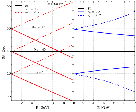
Figure 1: Evolution of $\theta^{m}_{23}$ in matter (given in Eq. 18) as a function of neutrino energy in the presence of SI and SI+NSI. Solid black curve in each panel represents the SI case while the other curves correspond to the SI+NSI cases with positive (solid lines) and negative (dashed lines) values of NSI parameters. In the left column, we show the running in the presence of NSI parameter $(\gamma-\beta)$, while the right column depicts the effect of $\varepsilon_{\mu\tau}$. We consider $L$ = 1300 km and assume NMO. We present results for three different values of $\theta_{23}$ in vacuum: $40^{\circ}$ (lower octant), $45^{\circ}$ (maximal value), $50^{\circ}$ (upper octant). The values of the other oscillation parameters in vacuum are taken from Table 2.

Approximate analytical expression describing the evolution of the effective mixing angle $\theta^{m}_{23}$ is given in Eq. 18. We can further simplify this expression by neglecting the small terms which are proportional to $\alpha s_{13}\sim 10^{-3}$ in Eq. 18, which enable us to extract the useful physics insights related to the running of $\theta^{m}_{23}$ in a more concise fashion. With this approximation, the expression showing the evolution of $\theta_{23}$ in matter in the presence of NSI takes the form

$$\tan 2\theta^{m}_{23}\simeq\frac{(c^{2}_{13}-\alpha c^{2}_{12})\sin 2\theta_{23}+2\varepsilon_{\mu\tau}\hat{A}}{(c^{2}_{13}-\alpha c^{2}_{12})\cos 2\theta_{23}+(\gamma-\beta)\hat{A}},$$ (24)

where, $\gamma-\beta=\varepsilon_{\tau\tau}-\varepsilon_{\mu\mu}$. Two important features emerge from this simplified expression.

• Only NSI parameters from the (2,3) block ($\varepsilon_{\mu\tau}$ and an effective NSI parameter $\gamma-\beta\equiv\varepsilon_{\tau\tau}-\varepsilon_{\mu\mu}$) of the NSI Hamiltonian contribute to the running of $\theta^{m}_{23}$.

• In the limiting case of all NSI parameters equal to zero (which in this case removes the standard matter effect $\hat{A}$ also), one would get back the vacuum mixing angle (i.e., $\theta_{23}^{m}=\theta_{23}$) irrespective of energy, baseline, and the octant of $\theta_{23}$. In other words, it implies that $\theta_{23}^{m}$ does not run in the presence of standard matter effect. Note that, in the exact expression of $\theta_{23}^{m}$ in Eq. 18, due to the presence of the tiny terms proportional to $\alpha s_{13}$, $\theta_{23}^{m}$ slightly deviates from its vacuum value even in the presence of SI.

In Fig. 1, we show the running of $\theta_{23}^{m}$ (using Eq. 18) with energy in presence of NSI parameters $(\gamma-\beta)$, $\varepsilon_{\mu\tau}$, taken one-at-a-time for a baseline corresponding to the DUNE experiment i.e. 1300 km. The left column shows the effect of NSI parameter $(\gamma-\beta)$ while the right column corresponds to the effect of $\varepsilon_{\mu\tau}$. The black curves in each column depict the SI case for three possible values of $\theta_{23}$ in vacuum, namely higher octant ($\theta_{23}=50^{\circ}$), maximal mixing ($\theta_{23}=45^{\circ}$), and lower octant ($\theta_{23}=40^{\circ}$). As discussed above, value of $\theta_{23}^{m}$ in SI case remains almost equal to the value of $\theta_{23}$ in vacuum. Only very small deviations from the vacuum value of $\theta_{23}$ can be observed due to the presence of terms proportional to $\alpha s_{13}$ in Eq. 18, which are neglected in Eq. 24. The solid (dashed) red curves in the left column of Fig. 1 illustrate the presence of $(\gamma-\beta)$ with a benchmark value of 0.2 (-0.2). We observe that for all the three values of $\theta_{23}$ mentioned above, $\theta_{23}^{m}$ monotonically decreases (increases) with energy when $(\gamma-\beta)$ is present with a positive (negative) value. In the right column, the solid (dashed) blue curves depict the case when only $\varepsilon_{\mu\tau}$ is present with a benchmark value of 0.2 (-0.2). Interestingly in lower (higher) octant, $\theta_{23}^{m}$ increases (decreases) for a positive value of $\varepsilon_{\mu\tau}$. For maximal mixing, the running of $\theta_{23}^{m}$ with energy is negligible in the presence of $\varepsilon_{\mu\tau}$ and remains almost equal to its vacuum value of $45^{\circ}$ (since the denominator of Eq. 24 vanishes). The dependence of $\theta_{23}^{m}$ running on the choice of octant of $\theta_{23}$ in vacuum can be understood from the fact that $\cos 2\theta_{23}$ in the denominator of the R.H.S. of Eq. 24 changes sign when $\theta_{23}$ lies in different octants.

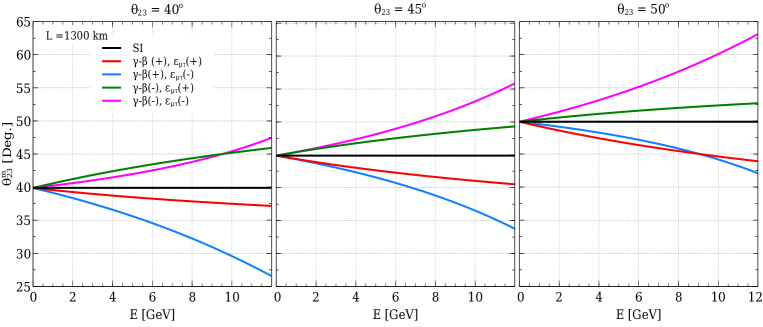
Figure 2: Evolution of $\theta^{m}_{23}$ (given in Eq. 18) with neutrino energy in matter with SI and NSI considering both $(\gamma-\beta)$ and $\varepsilon_{\mu\tau}$ non-zero at-a-time. Black curve in each column represents the SI case while the other curves show the cases with four possible combinations of the sign of $(\gamma-\beta)$ and $\varepsilon_{\mu\tau}$ with magnitude 0.2. The left, middle, and right column correspond to the evolution considering three values of $\theta_{23}$ in vacuum, $40^{\circ}$, $45^{\circ}$, and $50^{\circ}$, respectively. We consider $L$ = 1300 km and assume NMO. Values of the oscillation parameters in vacuum used in this plot are taken from Table 2.

Fig. 2 shows the running of $\theta^{m}_{23}$ when both the NSI parameters $\varepsilon_{\mu\tau}$ and $(\gamma-\beta)$ are non-zero. The four colored curves in each panel illustrate the effect of the four possible sign combinations of $(\gamma-\beta)$ and $\varepsilon_{\mu\tau}$ while the black curve shows the SI (with standard matter effect and no NSI) case, as shown in the legend. As before, three scenarios of the vacuum mixing angle $\theta_{23}$ are considered: higher octant ($\theta_{23}=50^{\circ}$), maximal mixing ($\theta_{23}=45^{\circ}$), and lower octant ($\theta_{23}=40^{\circ}$). We note from Fig. 2 that in the presence of $(\gamma-\beta)$ with a negative (positive) sign, $\theta_{23}^{m}$ monotonically increases (decreases) with energy irrespective of the sign of $\varepsilon_{\mu\tau}$ and the octant of $\theta_{23}$. We also observe that for lower (higher) octant, the decrease (increase) is the steepest when $(\gamma-\beta)$ is positive (negative) with negative value of $\varepsilon_{\mu\tau}$. For maximal mixing, the running of $\theta_{23}^{m}$ appears symmetric around the SI case since the term with $\cos 2\theta_{23}$ in the denominator of Eq. 18 vanishes.

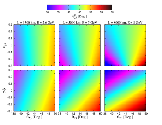
Figure 3: The evolution of of $\theta_{23}^{m}$ are shown in the plane of [$\theta_{23}-\varepsilon_{\mu\tau}$] (top row) and [$\theta_{23}-(\gamma-\beta)$] (bottom row). The left, middle, and right columns correspond to three sets of baseline and neutrino energy, namely (1300 km, 2.6 GeV), (5000 km, 5 GeV), and (8000 km, 8 GeV), respectively. Values of the oscillation parameters in vacuum used in this plot are taken from Table 2 and we assume NMO.

To show a correlation between NSI strength and the value of $\theta_{23}$ in vacuum, we have shown in Fig. 3, the evolution of $\theta_{23}^{m}$ in the plane of [$\theta_{23}-\varepsilon_{\mu\tau}$] (top panels) and [$\theta_{23}-(\gamma-\beta)$] (bottom panels). We demonstrate the effect of baseline by choosing three different baseline lengths as 1300 km, 5000 km, and 8000 km in the three columns, respectively. For each baseline, the energy is chosen as the corresponding value near the first oscillation maximum ($E_{\text{max}}$) for $\nu_{\mu}\to\nu_{e}$ oscillation. For the baseline of 1300 km, we see that $\theta_{23}^{m}$ decreases (increases) from the vacuum value ($\theta_{23}$) for a positive (negative) $\varepsilon_{\mu\tau}$ at higher octant. However, an opposite trend can be observed at lower octant. For maximal mixing, $\theta_{23}^{m}$ does not change in presence of $\varepsilon_{\mu\tau}$ only. These features are more pronounced for higher baselines since the NSI effect (proportional to matter density) gets enhanced. In the bottom row, in the presence of positive (negative) value of $(\gamma-\beta)$, $\theta_{23}^{m}$ decreases (increases) from the vacuum value, irrespective of the octant or maximal mixing. Larger baselines manifest it more clearly as evident from the steeper slant of the boundaries between different colors.

As mentioned earlier, we have assumed normal mass ordering (NMO) for our analysis. In case of inverted mass ordering (IMO) with neutrino ($\nu$, IMO), the effect of each NSI parameters in $\theta_{23}^{m}$ running is reversed (i.e., if $\theta^{m}_{23}$ increases with energy in presence of a particular NSI parameter with normal ordering of mass, in case of inverted mass ordering $\theta_{23}^{m}$ will decrease with energy). This happens since the term $\hat{A}$ associated with each NSI parameter changes its sign in case of IMO. Also, in case of antineutrino propagation with inverted mass ordering ($\bar{\nu}$, IMO), running of $\theta_{23}^{m}$ is almost the same as that of neutrino propagation with NMO ($\nu$, NMO). This is because of the fact that in both cases, sign of $\hat{A}$ is the same.

4.2 Running of $\theta_{13}^{m}$

Eq. 19 shows the running of $\theta_{13}^{m}$ in matter with NSI. We note that all five NSI parameters as well as the standard matter effect ($\hat{A}$) have impact on the running of $\theta_{13}^{m}$. It is observed that the value of $\theta_{23}$ in vacuum (when it is between $40^{\circ}$ and $50^{\circ}$) has a very small effect on the running of $\theta_{13}^{m}$. So, we simplify the expression for our understanding by assuming that the mixing angle $\theta_{23}$ in vacuum is maximal i.e., $45^{\circ}$. The relevant expression for the running of $\theta_{13}^{m}$ thus becomes,

$$\tan 2\theta^{m}_{13}\simeq\frac{\sin 2\theta_{13}(1-\alpha{s_{12}}^{2})(s^{m}_{23}+c^{m}_{23})-\alpha\sin 2\theta_{12}c_{13}(c^{m}_{23}-s^{m}_{23})+2\sqrt{2}(\varepsilon_{e\mu}s^{m}_{23}+\varepsilon_{e\tau}c^{m}_{23})\hat{A}}{\sqrt{2}(\lambda_{3}-\hat{A}-\alpha s^{2}_{12}c^{2}_{13}-s^{2}_{13})},$$ (25)

where,

$$\lambda_{3}=\frac{1}{2}\bigg{[}{c_{13}}^{2}+\alpha{c_{12}}^{2}+\alpha s^{2}_{12}s^{2}_{13}+(\beta+\gamma)\hat{A}+\frac{(\gamma-\beta)\hat{A}+\alpha\sin 2\theta_{12}s_{13}}{\cos 2\theta^{m}_{23}}\bigg{]}.$$ (26)

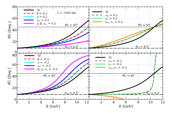
Figure 4: Evolution of $\theta_{13}^{m}$ (given in Eq. 25) with energy in presence of SI and NSI in matter. The solid black curve in each panel shows the SI case while the other curves correspond to the running in presence of SI+NSI. In the top (bottom) row, the NSI have been considered with a benchmark value of 0.2 (- 0.2). The left column depicts the presence of NSI parameters in (2,3) block while the right column shows the effect of $\varepsilon_{e\mu}$ and $\varepsilon_{e\tau}$. We have used $L$ = 1300 km and assumed NMO in the plot. Values of oscillation parameters in vacuum are given in Table 2 with $\theta_{23}=45^{\circ}$.

In Fig. 4, we show the running of $\theta_{13}^{m}$ with energy (by using Eqs. 25 and 26) in presence of NSI for a baseline of 1300 km and $\theta_{23}=45^{\circ}$. The SI case is depicted by the black curve in each panel and the other colored curves indicate the presence of NSI parameters in matter with a benchmark strength of 0.2 and -0.2. In the top row, we have shown the $\theta_{13}^{m}$ running when NSI are positive. The top left panel illustrates the presence of NSI parameters in (2,3) block while the right shows the effect of $\varepsilon_{e\mu}$ and $\varepsilon_{e\tau}$. We note that unlike the case of $\theta_{23}^{m}$, $\theta_{13}^{m}$ runs even in presence of only SI - its value rapidly rising with energy from the vacuum value of $\theta_{13}=8.5^{\circ}$. This can be understood from the fact that with an increase in energy, the term ($\lambda_{3}-\hat{A}$) in the denominator of the R.H.S. in Eq. 25 becomes smaller. The NSI parameters from (2,3) block suppress the rapid rise to some extent due to the modification in the value of $\lambda_{3}$ (see Eq. 26). Moreover, presence of $\beta$ or $\gamma$ only with the same strength, makes $\theta_{13}^{m}$ run in identical manner. On the other hand, $\varepsilon_{e\mu}$ and/or $\varepsilon_{e\tau}$ increases the magnitude of $\theta_{13}^{m}$ due to the additional contribution in the numerator of the R.H.S. in Eq. 25. For the case of maximal mixing of $\theta_{23}$, the impact of $\varepsilon_{e\mu}$ is identical to that of $\varepsilon_{e\tau}$ since $\theta_{23}^{m}\simeq\theta_{23}=45^{\circ}$. At lower energy, the gap between the curves showing running in presence of $\varepsilon_{e\mu}/\varepsilon_{e\tau}$ and the SI case increase with energy. However, as the value of $\theta_{13}^{m}$ approaches $45^{\circ}$, the gap becomes narrower and at $\theta_{13}^{m}=45^{\circ}$, these three curves intersect. It happens because, around value of $\theta_{13}^{m}\approx 45^{\circ}$ denominator of RHS in Eq. 25 becomes so small that the effect from the numerator which have $\varepsilon_{e\mu}/\varepsilon_{e\tau}$ is insignificant. In the bottom row, we have shown $\theta_{13}^{m}$ running for the negative values of the NSI parameters. It is clear from the bottom left panel that running of $\theta_{13}^{m}$ is enhanced when NSI from (2,3) block is present with negative strength. This happens since the presence of these negative NSI parameters decrease the value of $\lambda_{3}$, thereby decreasing the overall value of the denominator of R.H.S in Eq. 25. In the bottom right panel, some non-trivial effects are observed. We see that negative $\varepsilon_{e\mu}$ or $\varepsilon_{e\tau}$ highly suppresses the running of $\theta_{13}^{m}$ such that at lower energy ($E$ $\lesssim$ 6 GeV), it is almost constant when only one of them is present. It can be explained by the fact that both numerator and denominator of R.H.S. in Eq. 25 decreases with energy when $\varepsilon_{e\mu}$ and/or $\varepsilon_{e\tau}$ are negative, such that the overall value of $\theta_{13}^{m}$ remains almost constant at that energy range. However, at higher energy ($\sim$ 10 GeV) value of the denominator is so small that the overall effect led to the rapid increase in the magnitude of $\theta_{13}^{m}$ with energy. As we can see from Eq. 25, in presence of both $\varepsilon_{e\mu}$ and $\varepsilon_{e\tau}$ with a negative sign, the numerator decreases faster with energy compared to the previous case due to the additive effect of two NSI parameters. Consequently, value of $\theta_{13}^{m}$ decreases with energy from its vacuum value, and becomes negative (at $E$ $\gtrsim$ 6 GeV) when the numerator becomes negative.

In the case of IMO, the behavior of $\theta_{13}^{m}$ in SI as well as in SI+NSI case is significantly different from the NMO case for neutrino. It can be understood from the ($\lambda_{3}-\hat{A}$) term in the denominator of Eq. 25. Since $\hat{A}$ changes its sign, the denominator increases with energy, consequently the value of the $\theta_{13}^{m}$ decreases from its vacuum value. However, in case of antineutrino ($\bar{\nu}$) propagation and inverted mass ordering ($\bar{\nu}$, IMO), since $\hat{A}$ does not change its sign, running of $\theta_{13}^{m}$ is almost similar to neutrino ($\nu$, NMO) case.

4.3 Running of $\theta_{12}^{m}$

Similar to the case of $\theta_{13}^{m}$, value of $\theta_{23}$ in vacuum (when it is between $40^{\circ}$ and $50^{\circ}$) also has very small impact in the running of $\theta_{12}^{m}$. With the assumption of maximal mixing of $\theta_{23}$, the relevant expression for $\theta_{12}^{m}$ in Eq. 20 takes the form

$$\tan 2\theta^{m}_{12}\simeq\frac{{c^{m}_{13}}\big{[}\alpha\sin 2\theta_{12}c_{13}(c^{m}_{23}+s^{m}_{23})+\sin 2\theta_{13}(1-\alpha s_{12}^{2})(c^{m}_{23}-s^{m}_{23})+2\sqrt{2}(\varepsilon_{e\mu}c^{m}_{23}-\varepsilon_{e\tau}s^{m}_{23})\hat{A}\big{]}}{\sqrt{2}(\lambda_{2}-\lambda_{1})},$$ (27)

where,

$$\lambda_{2}=\frac{1}{2}\bigg{[}\alpha c^{2}_{12}+c^{2}_{13}+\alpha s^{2}_{12}s^{2}_{13}+(\beta+\gamma)\hat{A}-\frac{(\gamma-\beta)\hat{A}+\alpha\sin 2\theta_{12}s_{13}}{\cos 2\theta^{m}_{23}}\bigg{]},$$ (28)

$$\lambda_{1}=\frac{1}{2}\Big{[}\lambda_{3}+\hat{A}+s^{2}_{13}+\alpha s^{2}_{12}c^{2}_{13}-\frac{\lambda_{3}-\hat{A}-s^{2}_{13}-\alpha s^{2}_{12}c^{2}_{13}}{\cos 2\theta^{m}_{13}}\Big{]}.$$ (29)

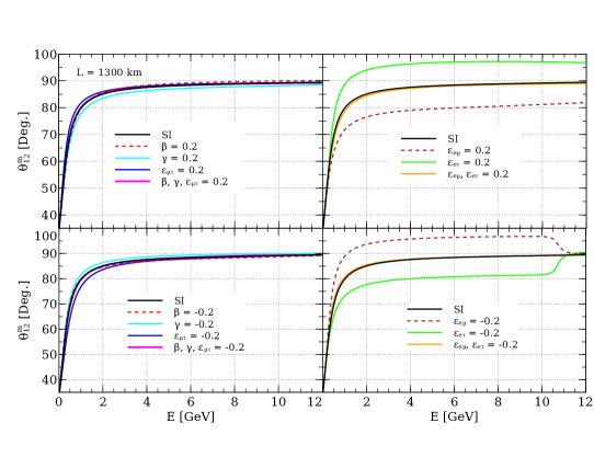
Figure 5: Evolution of $\theta_{12}^{m}$ (given in Eq. 27) with energy in presence of SI and NSI in matter. The solid black curve in each panel shows the SI case while the other curves correspond to the running in the presence of SI+NSI. In the top (bottom) row, the positive (negative) values of the NSI are considered with a benchmark value of 0.2 (-0.2). The left column depicts the presence of NSI parameters in (2,3) block while the right shows the effect of $\varepsilon_{e\mu}$ and $\varepsilon_{e\tau}$. We consider $L$ = 1300 km and assume NMO to prepare this plot. Values of oscillation parameters in vacuum used in this plot are taken from Table. 2 with $\theta_{23}=45^{\circ}$.

In Fig. 5, the running of $\theta_{12}^{m}$ with energy is shown both for SI (black curve) and for SI+NSI parameters (other curves) for a baseline of 1300 km and $\theta_{23}=45^{\circ}$. The left column shows the effect of the NSI parameters in (2,3) block, while the right column depicts the case of $\varepsilon_{e\mu}$ and $\varepsilon_{e\tau}$ with a strength of 0.2 or -0.2. For SI, at small energies ($E\lesssim 1.5-2$ GeV), $\lambda_{1}$ being close to $\lambda_{2}$, $\theta_{12}^{m}$ shows a very steep increase and then quickly saturates and approaches to $90^{\circ}$ approximately. Saturation occurs due to the following two reasons.

1. With increase in energy, $\lambda_{1}$ moves away from $\lambda_{2}$, resulting in a large denominator in the R.H.S. of Eq. 27.

2. $\theta_{13}^{m}$ rises with energy (see Fig. 4 and the relevant discussions in Subsec. 4.2) and so the overall factor $c_{13}^{m}$ in Eq. 27 decreases.

In the presence of NSI parameters in (2,3) block, $\lambda_{1}$, $\lambda_{2}$ and $c^{m}_{13}$ undergo mild change, - retaining almost the same features as that of SI. The presence of $\varepsilon_{e\mu}$ ($\varepsilon_{e\tau}$) however, adds up to the numerator of Eq. 27 and the value of $\theta_{12}^{m}$ at which it saturates, shifts down (up). When both $\varepsilon_{e\mu}$ and $\varepsilon_{e\tau}$ are present, they cancel their effect due to the relative sign between them and the running of $\theta_{12}^{m}$ almost coincides with SI scenario. In the bottom row, we have shown the running of $\theta_{12}^{m}$ for the NSI with negative strength. Since running of $\theta_{12}^{m}$ very mildly depend on NSI parameters from the (2,3) sector (bottom left panel), the sign of these NSI parameters do not have any significant effect. In the bottom right panel, we see that role of $\varepsilon_{e\mu}$ and $\varepsilon_{e\tau}$ is reversed when the sign of the NSI parameter is changed. Interestingly, at energies around 10 GeV, sudden decrease (increase) of $\theta_{12}^{m}$ can be observed in the presence of NSI parameter $\varepsilon_{e\mu}$ ($\varepsilon_{e\tau}$) with negative strength. It happens due to the presence of the term $\cos\theta_{13}^{m}$ in the numerator of the R.H.S. of Eq. 27, which reduces rapidly to a very small value around that energy (see Fig. 4 and related discussion in Subsec. 4.2).

Unlike $\theta_{13}^{m}$, the $\theta_{12}^{m}$ running shows similar behavior in SI as well as in SI+NSI cases for neutrino propagation with IMO ($\nu$, IMO). Also, it shows completely different behavior in case of antineutrino propagation with inverted mass ordering ($\bar{\nu}$, IMO). It can be understood from the fact that in case of IMO, sign of first and third terms in the numerator of Eq. 27 gets flipped, and in the denominator, the sign of $\lambda_{1}$ gets changed. Since the effect from other remaining terms are very small, both numerator and denominator change their sign, and as a result, $\theta_{12}^{m}$ remains the same as in the case of ($\nu$, NMO). In case of ($\bar{\nu}$, IMO), only first term in the numerator changes its sign, $\lambda_{1}$ in the denominator remains the same as in case of ($\nu$, NMO). As a result, we see a completely different behavior of $\theta_{12}^{m}$.

5 Evolution of Mass-Squared Differences in the presence of NSI

After the diagonalization of the effective propagation Hamiltonian $H_{f}$ in Sec. 2, we obtain the expressions for the eigenvalues $m^{2}_{i,m}/2E$ ($i=1,2,3$):

$$\frac{m^{2}_{3,m}}{2E}\simeq \frac{\Delta_{31}}{2}\Big{[}\lambda_{3}+\hat{A}+s^{2}_{13}+\alpha s^{2}_{12}c^{2}_{13}+\frac{\lambda_{3}-\hat{A}-s^{2}_{13}-\alpha s^{2}_{12}c^{2}_{13}}{\cos 2\theta^{m}_{13}}\Big{]}\,,$$ (30)

$$\frac{m^{2}_{2,m}}{2E}\simeq \frac{\Delta_{31}}{2}\Big{[}\lambda_{1}+\lambda_{2}-\frac{\lambda_{1}-\lambda_{2}}{\cos 2\theta^{m}_{12}}\Big{]}\,,$$ (31)

$$\frac{m^{2}_{1,m}}{2E}\simeq \frac{\Delta_{31}}{2}\Big{[}\lambda_{1}+\lambda_{2}+\frac{\lambda_{1}-\lambda_{2}}{\cos 2\theta^{m}_{12}}\Big{]}\,,$$ (32)

where, we assume $\theta_{23}=45^{\circ}$ and we are already familiar with the expressions of $\theta^{m}_{ij}$ and $\lambda_{i}$. Using the above equations, we can obtain the approximate analytical expressions for the modified mass-squared differences $\Delta m^{2}_{31,m}\equiv m^{2}_{3,m}-m^{2}_{1,m}$ and $\Delta m^{2}_{21,m}\equiv m^{2}_{2,m}-m^{2}_{1,m}$. The behavior of $\Delta m^{2}_{31,m}$ ($\Delta m^{2}_{21,m}$) is mainly governed by $m^{2}_{3,m}$ ($m^{2}_{2,m}$). This is due to the fact that in the approximation $\theta_{12}^{m}$ saturating to $90^{\circ}$ (see Subsec. 4.3), $m^{2}_{2,m}\approx\lambda_{1}\Delta_{31}$ and $m^{2}_{1,m}\approx\lambda_{2}\Delta_{31}$. Therefore, $\lambda_{2}$ being very small, $m^{2}_{1,m}$ is insignificant.

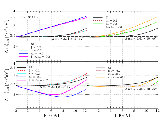
Figure 6: Variation of $\Delta m^{2}_{31,m}$ ($\equiv m^{2}_{3,m}-m^{2}_{1,m}$) as obtained from Eqs. 30-32 is shown with energy in SI case and SI+NSI cases. Top (bottom) row corresponds to the positive (negative) NSI with strength 0.2. The solid black curve in each panel shows the SI case while the other curves show the running in presence of NSI. The left column depicts the presence of various NSI parameters in (2,3) block while the right shows the effect of $\varepsilon_{e\mu}$ and $\varepsilon_{e\tau}$. We consider $L=1300$ km and the values of the oscillation parameters used in this plot are taken from Table 2. We assume $\theta_{23}=45^{\circ}$ and NMO.

In Fig. 6, we show the running of $\Delta m^{2}_{31,m}$ both for SI (black curve) and SI+NSI (other colored curves) scenarios. The top (bottom) row corresponds to the running in the presence of positive (negative) NSI with strength 0.2. The left column depicts the presence of various NSI parameters in (2,3) block while the right shows the effect of $\varepsilon_{e\mu}$ and $\varepsilon_{e\tau}$. A baseline of 1300 km and a maximal mixing for $\theta_{23}$ is considered. For the SI case, $\Delta m^{2}_{31,m}$ first increases very slowly with energy and then with a relatively steeper rate (around $E\gtrsim 9$ GeV). This is due to the additive contribution of the last term in Eq. 30 when $\theta_{13}^{m}$ increases rapidly with energy. In the top left panel, presence of $\beta$ or $\gamma$ shows a similar running of $\Delta m^{2}_{31,m}$ while the introduction of $\varepsilon_{\mu\tau}$ shows a steady and almost linear increase with energy due to the increase of $\lambda_{3}$ appearing in R.H.S. of Eq. 30. In the top right panel, the presence of $\varepsilon_{e\mu}$ or $\varepsilon_{e\tau}$ shows identical effects and makes $\Delta m^{2}_{31,m}$ rise with a steeper rate. Both $\varepsilon_{e\mu}$ and $\varepsilon_{e\tau}$ when present together generate an additive effect and further elevates the steepness of $\Delta m^{2}_{31,m}$. In the bottom row, we show the running in the presence of negative NSI with strength 0.2. Presence of $\beta$ or $\gamma$ with flipped signs reverse the behavior of $\Delta m^{2}_{31,m}$. In presence of negative $\varepsilon_{\mu\tau}$, initially, there is a steady decrease in the value of $\Delta m^{2}_{31,m}$ because of the decreasing behavior of $\lambda_{3}$. However, at higher energy ($E\gtrsim$ 7 GeV), we see sudden growth in the running of $\Delta m^{2}_{31,m}$ due to increase in the value of $\theta_{13}^{m}$ at a faster rate which in turn increase the value of $m^{2}_{3,m}$. In the bottom right panel, we show the running in the presence of $\varepsilon_{e\mu}$ and/or $\varepsilon_{e\tau}$ with negative strength. In the presence of negative $\varepsilon_{e\mu}$ or $\varepsilon_{e\tau}$, the value of $\Delta m^{2}_{31,m}$ becomes almost constant initially ($E\lesssim 10.5$ GeV), which can be understood from the running of $\theta_{13}^{m}$ in the presence of negative NSI (bottom right panel of Fig. 4) and the fact that $\lambda_{3}$ is constant in the presence of $\varepsilon_{e\mu}$ or $\varepsilon_{e\tau}$. At $E\gtrsim$ 10 GeV, a sudden increase in the value of $\theta_{13}^{m}$ leads to the increasing behavior of $\Delta m^{2}_{31,m}$ around that energy.

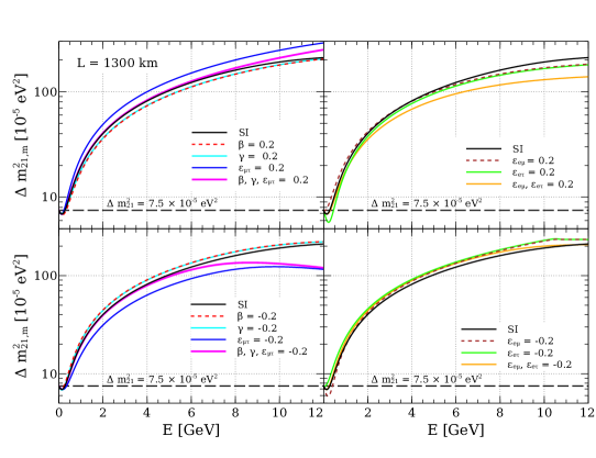
Figure 7: Variation of $\Delta m^{2}_{21,m}$ ($\equiv m^{2}_{2,m}-m^{2}_{1,m}$) as obtained from Eqs. 30-32 is shown with energy in SI case and SI+NSI cases. Top (bottom) row corresponds to the positive (negative) NSI with strength 0.2. The solid black curve in each panel shows the SI case while the other curves show the running in presence of NSI. The left column depicts the presence of various NSI parameters in (2,3) block while the right shows the effect of $\varepsilon_{e\mu}$ and $\varepsilon_{e\tau}$. We consider $L=1300$ km and the values of the oscillation parameters used in this plot are taken from Table 2. We assume $\theta_{23}=45^{\circ}$ and NMO.

In Fig. 7, we have shown the running of $\Delta m^{2}_{21,m}$ with energy for the baseline 1300 km and $\theta_{23}=45^{\circ}$. The black curve in each panel corresponds to the SI case while other curves show the running in presence of NSI. Top (Bottom) row corresponds to the running in the presence of positive (negative) NSI with strength 0.2. SI case shows steady increase with energy, - reaching a value of an order as high as $\gtrsim 10^{-3}\text{ eV}^{2}$ from its vacuum order of magnitude $10^{-5}\text{ eV}^{2}$. In other words, the running of $\Delta m^{2}_{21,m}$ can make itself comparable in magnitude with that of $\Delta m^{2}_{31,m}$. In the presence of positive (top row) or negative (bottom row) NSI (except for negative $\varepsilon_{\mu\tau}$ or taking negative $\beta,\gamma,\varepsilon_{\mu\tau}$ together), the behavior of $\Delta m^{2}_{21,m}$ does not show significant deviation in magnitude from SI case. But interestingly, depending on the sign of NSI parameter, the magnitude of $\Delta m^{2}_{21,m}$ in presence of NSI is slightly higher or lower than in presence of SI. In presence of negative $\varepsilon_{\mu\tau}$ (when present singly or together with negative $\beta$ and $\gamma$), we see a deviation from SI case at higher energy which can be understood from the variation of $\lambda_{1}$ with energy. With negative $\varepsilon_{e\mu}$ or $\varepsilon_{e\tau}$, however, at $E\gtrsim$ 10.5 GeV $\Delta m^{2}_{21,m}$ becomes almost constant. It happens due to a sudden increase in the value of $\theta_{13}^{m}$ around that energy which results in saturation of the value of $\lambda_{1}$.

In the case of IMO, running of $\Delta m^{2}_{21,m}$ is almost the same as ($\nu$, NMO) case for both neutrino and antineutrino propagation. However, IMO leads to a significant change in the running of $\Delta m^{2}_{31,m}$ for both neutrino and antineutrino propagation which is obvious because the vacuum value $\Delta m_{31}^{2}$ changes its sign.

6 $\theta_{13}$-Resonance in the presence of NSI

From the running of $\theta_{13}^{m}$ (Eq. 25), we see that interestingly there exists a resonance such that

$$\hat{A}=\lambda_{3}-\alpha s^{2}_{12}c^{2}_{13}-s^{2}_{13}\,.$$ (33)

Consequently, the denominator of the R.H.S. of Eq. 25 becomes close to zero and $\theta_{13}^{m}$ becomes maximal ($45^{\circ}$). We note that this resonance is independent of the value of $\varepsilon_{e\mu}$ or $\varepsilon_{e\tau}$ (as evident from the right panels of Fig. 4) but depends upon NSI parameters in the (2,3) block. We know that for the SI case, under the one mass scale dominance (OMSD) approximation ($\Delta m^{2}_{31}L/4E>>\Delta m^{2}_{21}L/4E$), the resonance occurs at an energy $E_{\text{res}}$ such that Akhmedov:2004ny ,

$$\left[E_{\text{res}}^{\text{SI}}\right]_{\text{OMSD}}=\frac{\Delta m^{2}_{31}\cos 2\theta_{13}}{2V_{CC}}\,,$$ (34)

where, $V_{CC}$ is the standard $W$-exchange interaction potential in matter (Eq. 7). In presence of NSI, we seek to find out the modifications in Eq. 34 considering $\theta_{23}=45^{\circ}$. After replacing $\cos 2\theta^{m}_{23}$ from Eq. 18 in the expression for $\lambda_{3}$ (Eq. 3), we obtain,

$$\lambda_{3} \simeq\frac{1}{2}\bigg{[}c^{2}_{13}+\alpha c^{2}_{12}+\alpha s^{2}_{12}s^{2}_{13}+(\beta+\gamma)\hat{A}$$

$$+\sqrt{\{\alpha s_{13}\sin 2\theta_{12}+(\gamma-\beta)\hat{A}\}^{2}+\{c^{2}_{13}-\alpha c^{2}_{12}+\alpha s^{2}_{12}s^{2}_{13}+2\varepsilon_{\mu\tau}\hat{A}\}^{2}}\bigg{]}\,.$$ (35)

In the above equation, we neglect the small terms proportional to $\alpha s^{2}_{13},(\gamma-\beta)^{2}\hat{A}^{2}$ and the cross-term proportional to $\alpha\hat{A}(\gamma-\beta)s_{13}$. Finally, we get the following simpler expression for $\lambda_{3}$,

$$\lambda_{3}\simeq c^{2}_{13}+\frac{1}{2}(\beta+\gamma+2\varepsilon_{\mu\tau})\hat{A}\,.$$ (36)

It is noteworthy to mention that for SI case, we get $\lambda_{3}\simeq c_{13}^{2}$. Putting this back in Eq. 33 and using OMSD approximation, we easily obtain the well-known expression for resonance in Eq. 34. Equating Eqs. 33 and 36, we obtain the following final expression for the resonance energy,

$$E_{\text{res}}^{\text{NSI}}\simeq\frac{\Delta m^{2}_{31}\cos 2\theta_{13}}{2V_{CC}}\bigg{[}\frac{1-(\alpha s^{2}_{12}c_{13}^{2}/\cos 2\theta_{13})}{1-\frac{1}{2}(\beta+\gamma+2\varepsilon_{\mu\tau})}\bigg{]}=\left[E_{\text{res}}^{\text{SI}}\right]_{\text{OMSD}}\bigg{[}\frac{1-(\alpha s^{2}_{12}c_{13}^{2}/\cos 2\theta_{13})}{1-\frac{1}{2}(\beta+\gamma+2\varepsilon_{\mu\tau})}\bigg{]}.$$ (37)

The term in the square bracket in the R.H.S. of Eq. 37 is the correction over Eq. 34. The term $\frac{1}{2}(\beta+\gamma+2\varepsilon_{\mu\tau})$ is the correction induced by the presence of NSI, while $\alpha s^{2}_{12}c_{13}^{2}/\cos 2\theta_{13}$ is the modification induced by relaxing the OMSD approximation. Thus it is now also clear analytically that $\theta_{13}^{m}$-resonance gets affected only by the NSI parameters in the (2,3) block and not by $\varepsilon_{e\mu}$ or $\varepsilon_{e\tau}$.

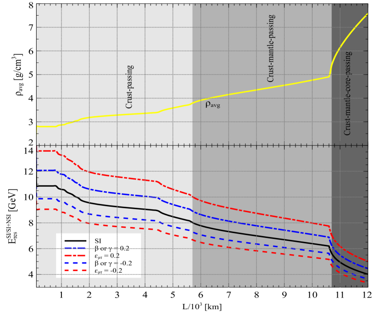
Figure 8: Behavior of the $\theta_{13}$-resonance energy (Eq. 37) with baseline length ($L$) inside the Earth. Upper panel shows the line-averaged constant Earth matter density for a given baseline obtained using the PREM profile. Lower panel shows the value of the resonance energy ($\theta_{13}^{m}=45^{\circ}$) corresponding to each baseline length $L$ inside the Earth in SI case (solid black line), SI + non-zero positive NSI case (dot-dashed lines), and SI + non-zero negative NSI case (dashed lines) considering one NSI parameters at-a-time as shown in the legends. The values of the oscillation parameters used in this plot are taken from Table 2. We assume $\theta_{23}=45^{\circ}$ and NMO.

Fig. 8 (bottom panel) shows $E^{\text{NSI}}_{\text{res}}$ as a function of baseline length for SI case (black solid curve) and in presence of NSI (other colored lines). The dot-dashed (dashed) curves depict the case of positive (negative) NSI parameters as indicated by the legends. The top panel of Fig. 8 shows the line-averaged constant Earth matter density ($\rho_{\text{avg}}$) for a given baseline $L$ obtained from the PREM profile Dziewonski:1981xy . In both the panels of Fig. 8, we indicate by three gray shades, the baselines when it touches the three interior layers of the Earth: crust, mantle, and core. Since $\rho_{\text{avg}}$ shows an increase in magnitude (thus increasing $V_{CC}$ in Eq. 37) with $L$, the values of $E_{\text{res}}^{\text{NSI}}$ itself decreases with $L$, following similar pattern (for both SI and NSI). As it is also clear from Eq. 37, a positive (negative) value of the NSI parameters $\beta,\gamma$, or $\varepsilon_{\mu\tau}$ shifts the magnitude of $E_{\text{res}}^{\text{NSI}}$ to a higher (lower) value than the SI case. Eq. 37 also tells us, if it turns out that the NSI parameters are present in Nature with such magnitudes that $\beta+\gamma=-2\varepsilon_{\mu\tau}$, then the correction due to NSI vanishes. In that case, if we ignore the minor correction induced by $\alpha s^{2}_{12}c_{13}^{2}/\cos 2\theta_{13}$ term we obtain, $E_{\text{res}}^{\text{NSI}}\simeq E_{\text{res}}^{\text{SI}}$.

7 Impact of NSI in $\nu_{\mu}-\nu_{e}$ appearance channel

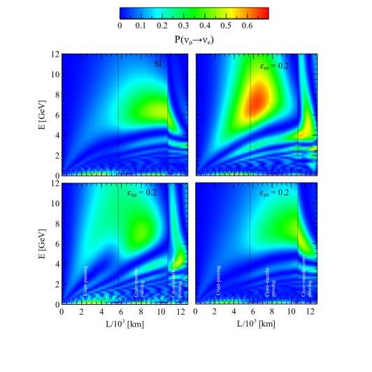
Figure 9: Oscillograms of $\nu_{\mu}\rightarrow\nu_{e}$ transition probability as a function of baseline $L$ and energy $E$. Top left panel corresponds to SI case and other three panels correspond to the cases in presence of non-zero positive NSI parameters (taken one-at-a-time with a strength of 0.2 as shown in the legends). The values of the oscillation parameters used in this plot are taken from Table 2 with $\theta_{23}=45^{\circ}$ and NMO.

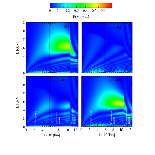
Figure 10: Oscillogram of $\nu_{\mu}\rightarrow\nu_{e}$ transition probability as a function of baseline $L$ and energy $E$. Top left panel corresponds to SI case and other three panels correspond to the cases in presence of non-zero negative NSI parameters (taken one-at-a-time with a strength of 0.2 as shown in the legends). The values of the oscillation parameters used in this plot are taken from Table 2 with $\theta_{23}=45^{\circ}$ and NMO.

One of the most important oscillation channel that is probed in LBL experiment is $\nu_{\mu}\rightarrow\nu_{e}$ appearance channel. This channel will play a significant role in determining the value of the CP phase, neutrino mass ordering, octant of $\theta_{23}$ from various upcoming neutrino oscillation experiments. So, in this section, we are interested in studying the effect of NSI on $\nu_{\mu}\to\nu_{e}$ transition probability maxima at various baselines ($L$) through the Earth-matter with neutrino beam having energy ($E$) in the GeV range. In order to study this, in Fig. 9, we plot the $\nu_{\mu}\rightarrow\nu_{e}$ transition probability in $(E$ - $L)$ plane in SI case and SI+NSI cases considering a benchmark value of 0.2 for the strength of the NSI parameters. We use the vacuum probability expression for $\nu_{\mu}\to\nu_{e}$ appearance Agarwalla:2013tza and replace the vacuum oscillation parameters with their modified counterparts in matter with SI and NSI (Eqs. 18-20 and Eqs. 30-32) and use this modified probability expression for plotting Fig. 9. $\theta_{23}$ in vacuum is considered to be maximal. We check that Fig. 9 shows very good agreement in both SI and SI+NSI cases with the exact three-flavor oscillation probabilities which are calculated numerically using the GLoBES software Huber:2004ka ; Huber:2007ji . Top left panel shows the SI case where no NSI are taken into account. Here, it is observed that the region of maximum appearance probability occurs for the baseline almost passing through the core and the mantle boundary. However, in presence of $\varepsilon_{e\mu}$ (bottom left panel) or $\varepsilon_{e\tau}$ (top right panel) this region shifts towards lower baselines. In case of $\varepsilon_{\mu\tau}$ (bottom right panel), this region remains almost the same as in the SI case. To show the effect of NSI with negative strength, we similarly plot the oscillograms in Fig. 10 in SI case and in the presence of negative NSI with strength 0.2. Huge differences in the oscillation patterns can be observed in case of $\varepsilon_{e\mu}$ and $\varepsilon_{e\tau}$. Unlike Fig. 9, there is no such region of the maximum transition probability in Fig. 10.

In Fig. 9, we notice that for positive values of $\varepsilon_{e\mu}$ and $\varepsilon_{e\tau}$, a significant enhancement in the $\nu_{\mu}\rightarrow\nu_{e}$ transition probability as compared to SI case, for some choices of $L$ and $E$ where we have large matter effects. On the other hand, in Fig. 10, for negative choices of $\varepsilon_{e\mu}$ and $\varepsilon_{e\tau}$, we see a large depletion in $\nu_{\mu}\rightarrow\nu_{e}$ transition probability for some choices of $L$ and $E$ where matter effect is suppressed. Now, we make an attempt to understand these features with the help of approximate analytical expressions. After replacing the vacuum oscillation parameters with their modified counterparts in the $\nu_{\mu}\to\nu_{e}$ transition probability as mentioned above, we simplify it further by using the approximation that $\theta_{12}^{m}$ almost saturates to $\pi/2$ (see Fig. 5 and the related discussion in Subsec. 4.3). As a result, we obtain the following simplified expression that helps us to explain the broad features observed in Figs. 9 and 10,

$$P^{m}_{\nu_{\mu}\rightarrow\nu_{e}}=\underbrace{\sin^{2}\theta_{23}^{m}}_{T_{1}}\,\,\underbrace{\sin^{2}2\theta^{m}_{13}}_{T_{2}}\,\,\underbrace{\sin^{2}\bigg{[}\frac{1.27\times\Delta m^{2}_{32,m}L}{E}\bigg{]}}_{T_{3}}\,.$$ (38)

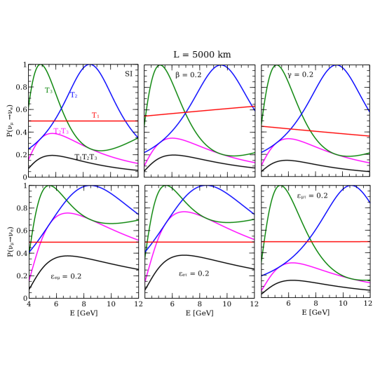
Figure 11: Variation of $\nu_{\mu}\rightarrow\nu_{e}$ transition probability (Eq. 38) with energy under the approximation $\theta_{12}^{m}\rightarrow 90^{\circ}$ for a baseline of $L$ = 5000 km. $T_{1}$ (red curve), $T_{2}$ (blue curve), and $T_{3}$ (green curve) are the three terms defined in Eq. 38. Various panels represent the SI case and SI+NSI cases as shown in the labels. To prepare this plot, the values of the three-flavor oscillation parameters are taken from Table 2. We assume $\theta_{23}=45^{\circ}$ and NMO.

In Fig. 11, we plot Eq. 38 with energy and also the contribution from each term $T_{1}$, $T_{2}$, and $T_{3}$, separately. It is clear from the figure that the variation of $T_{1}$ with energy is very less compared to the variation of $T_{2}$ and $T_{3}$. Thus, the energy at which maximum of $T_{1}T_{2}T_{3}$ occurs is the same as that of $T_{2}T_{3}$. In other words, the maximum of $P^{m}_{\nu_{\mu}\rightarrow\nu_{e}}$ occurs at an energy determined by $T_{2}$ and $T_{3}$, not $T_{1}$. This feature is also valid for any other baselines. So, $P^{m}_{\nu_{\mu}\rightarrow\nu_{e}}$ is maximum when both the following two conditions are satisfied simultaneously.

• $T_{2}\equiv\sin^{2}\theta^{m}_{13}=1$ i.e., $\theta_{13}^{m}=45^{\circ}$ ($\theta_{13}$-resonance condition). This condition is achieved in SI case when $E=E_{\text{res}}=\frac{\Delta m^{2}_{31}\cos 2\theta_{13}}{2V_{CC}}$ (see Eq. 34) with the OMSD approximation.

• $T_{3}\equiv\sin^{2}\bigg{[}\frac{1.27\times\Delta m^{2}_{32,m}L}{E}\bigg{]}=1$ for some energy $E=E^{m}_{\text{max}}$, such that

  $$E^{m}_{\text{max}}=\frac{1.27\times\Delta m^{2}_{32,m}L}{(2n+1)\pi/2}\quad\text{ with }n=0,1,2...$$ (39)

Thus, the maximum matter effect is obtained when the condition $E_{\text{res}}=E^{m}_{\text{max}}$ is satisfied Banuls:2001zn ; Gandhi:2004md ; Gandhi:2004bj .

In order to simplify the expression of $E^{m}_{\text{max}}$ in the presence of SI only, we use Eq. 30 and Eq. 31 to calculate $\Delta m^{2}_{32,m}$ considering all the NSI parameters to be zero. Applying the OMSD approximation and $\theta_{23}=45^{\circ}$, we obtain

$$\Delta m^{2}_{32,m}=\Delta m^{2}_{31}\sqrt{(\lambda_{3}-\hat{A}-s^{2}_{13})+\sin^{2}2\theta_{13}}\,.$$ (40)

Now, using Eq. 40 in the expression of $E^{m}_{\text{max}}$ in Eq. 39, the condition for the maximum matter effect $E_{\text{res}}=E^{m}_{\text{max}}$ gets further simplified. Ultimately, we obtain a simple and compact relation between the baseline ($L$) and the corresponding line-averaged constant matter density ($\rho_{\text{avg}}$) to have the maximum $\nu_{\mu}\rightarrow\nu_{e}$ transition probability in matter

$$\big{(}\rho_{\text{avg}}L\big{)}_{\text{SI}}=\frac{(2n+1)\times\pi\times 5.18\times 10^{3}}{\tan 2\theta_{13}}\hskip 2.84544pt\text{km g/cm${}^{3}$}\,.$$ (41)

Note that under the OMSD approximation, the resonance energy condition in Eq. 33 takes a very simple form: $(\lambda_{3}-\hat{A}-s^{2}_{13})=0$ and we make use of this expression in Eq. 40 to obtain Eq. 41, which exactly matches with the expression derived by the authors in Ref. Gandhi:2004md .

Now, we analyze how Eq. 41 gets modified in the presence of NC-NSI. First, we use Eqs. 3$-$23 and Eqs. 30$-$32 to derive the following two expressions for $m^{2}_{3,m}$ and $m^{2}_{2,m}$ under the OMSD approximation and assuming $\theta_{23}=45^{\circ}$.

$$m^{2}_{3,m} =\frac{\Delta m_{31}^{2}}{2}\big{[}\lambda_{3}+\hat{A}+s^{2}_{13}+T\big{]}\,,$$

$$m^{2}_{2,m} =\frac{\Delta m_{31}^{2}}{2}\big{[}\lambda_{3}+\hat{A}+s^{2}_{13}-T\big{]}\,,$$ (42)

where,

$$T=\frac{1}{\sqrt{2}}\sqrt{2\big{[}\lambda_{3}-\hat{A}-s^{2}_{13}\big{]}^{2}+\big{[}\sin 2\theta_{13}(c^{m}_{23}+s^{m}_{23})+2\sqrt{2}(\varepsilon_{e\mu}s^{m}_{23}+\varepsilon_{e\tau}c^{m}_{23})\big{]}^{2}}\,.$$ (43)

Using the resonance energy condition (Eq. 33), we now have

$$\Delta m^{2}_{32,m}=m^{2}_{3,m}-m^{2}_{2,m}=\Delta m_{31}^{2}\big{[}\frac{1}{\sqrt{2}}\sin 2\theta_{13}(c^{m}_{23}+s^{m}_{23})+2(\varepsilon_{e\mu}s^{m}_{23}+\varepsilon_{e\tau}c^{m}_{23})\big{]}\,.$$ (44)

Replacing $\Delta m^{2}_{32,m}$ in Eq. 39, we finally have the following condition for the maximal $\nu_{\mu}\rightarrow\nu_{e}$ transition probability in the presence of NC-NSI.

$$\big{(}\rho_{\text{avg}}L\big{)}_{\text{NSI}}$$

$$\simeq\frac{(2n+1)\pi\times 5.18\times 10^{3}}{\tan 2\theta_{13}\big{[}1-\big{\{}(\beta+\gamma+2\varepsilon_{\mu\tau})(\frac{c^{m}_{23}+s^{m}_{23}}{2\sqrt{2}})\big{\}}+\big{\{}2(\varepsilon_{e\mu}s^{m}_{23}+\varepsilon_{e\tau}c^{m}_{23})/\tan 2\theta_{13}\big{\}}\big{]}}\hskip 2.84544pt\text{km g/cm${}^{3}$}$$ (45)

$$=\big{(}\rho_{\text{avg}}L\big{)}_{\text{SI}}\bigg{[}\frac{1}{1-\big{\{}(\beta+\gamma+2\varepsilon_{\mu\tau})(\frac{c^{m}_{23}+s^{m}_{23}}{2\sqrt{2}})\big{\}}+\big{\{}2(\varepsilon_{e\mu}s^{m}_{23}+\varepsilon_{e\tau}c^{m}_{23})/\tan 2\theta_{13}\big{\}}}\bigg{]}\text{km g/cm${}^{3}$}.$$ (46)

The second factor in the R.H.S. of Eq. 7 is the correction introduced by the NSI parameters. As shown in Fig. 11, the modified $\theta_{23}^{m}$ does not run significantly and is also close to $45^{\circ}$ for maximal mixing of $\theta_{23}$. Using the approximation $\theta_{23}^{m}\simeq 45^{\circ}$, we simplify Eq. 7 to the following.

$$\big{(}\rho_{\text{avg}}L\big{)}^{max}_{\text{NSI}}\simeq\big{(}\rho_{\text{avg}}L\big{)}_{\text{SI}}\bigg{[}\frac{1}{1-\big{\{}(\beta+\gamma+2\varepsilon_{\mu\tau})\big{\}}/2+\big{\{}\sqrt{2}(\varepsilon_{e\mu}+\varepsilon_{e\tau})/\tan 2\theta_{13}\big{\}}}\bigg{]}\text{km g/cm${}^{3}$}\,.$$ (47)

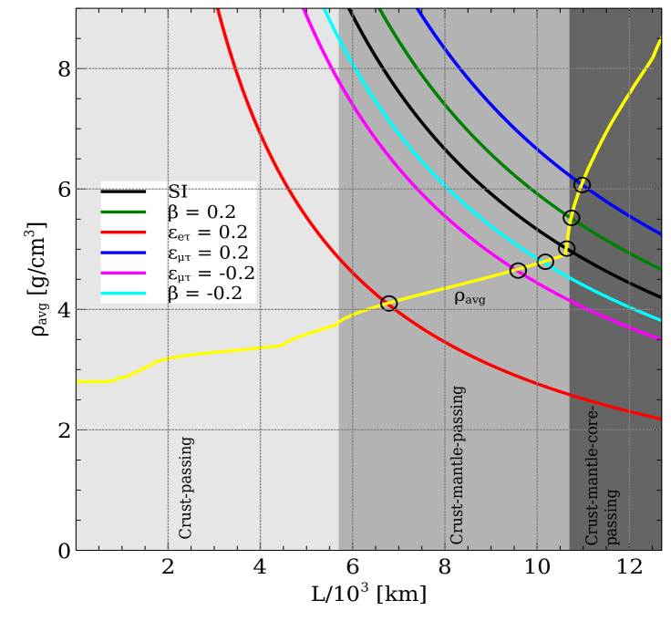
Figure 12: The solid yellow line shows the line-averaged constant Earth matter density (obtained using the PREM profile) for a given $L$. The intersection point of the solid black and yellow lines depict the value of $L$ and its corresponding $\rho_{avg}$ for which $\nu_{\mu}\rightarrow\nu_{e}$ transition probability attains the maximum value (see Eq. 41). The intersection points of the other solid lines with solid yellow line show the same considering one NSI parameter at-a-time (see the legends). The three-flavor oscillation parameters in vacuum are taken from Table 2 with a choice of $\theta_{23}=45^{\circ}$ and NMO.

In Fig. 12, we plot the R.H.S. of Eq. 47 in presence of SI and also in presence of NSI parameters ($\beta,\varepsilon_{\mu\tau},\varepsilon_{e\tau}$ taken one-at-a-time with a magnitude of 0.2) in the $\rho_{\text{avg}}$ and $L$ plane. In the presence of NSI parameter $\gamma$ ($\varepsilon_{e\mu}$), Eq. 47 is same as in the presence of $\beta$ ($\varepsilon_{e\tau}$). Again, three gray regions correspond to the baseline length passing through the crust, crust-mantle, and crust-mantle-core. In the same figure, we also show the line-averaged constant Earth matter density according to the PREM profile (yellow curve). The points of intersections of the hyperbolic curves (corresponding to Eq. 41 for the SI case and Eq. 47 for the SI+NSI cases) with the yellow curve give the baseline lengths, required to achieve the maximum of $P^{m}_{\nu_{\mu}\to\nu_{e}}$. When there are no NSI present in the scenario, the baseline length required for maximum transition probability is around 10600 km, which almost touches the core of the Earth. This same feature is also observed in the oscillogram plot in Fig. 9 which is plotted using full three-flavor $\nu_{\mu}\rightarrow\nu_{e}$ oscillation probability expression. When NSI parameters from (2,3) block with positive (negative) strength are present one-at-a-time, the required baseline length increases (decreases) slightly. But interestingly, when the NSI parameter $\varepsilon_{e\mu}$ or $\varepsilon_{e\tau}$ is present, the required baseline length for maximum $\nu_{\mu}\to\nu_{e}$ transition decreases drastically to around 6700 km (intersection between red and yellow curve in Fig. 12), which passes through only crust and mantle of the Earth.

It is evident from Eq. 47 that since the role of $\varepsilon_{e\mu}$ and $\varepsilon_{e\tau}$ are on the same footing, the presence of $\varepsilon_{e\mu}$ induces an effect identical to that of $\varepsilon_{e\tau}$ with the same magnitude. But the oscillograms (Figs. 9 and 10) for $\varepsilon_{e\mu}$ and $\varepsilon_{e\tau}$ look quite different. This is because of the fact that $\theta_{12}^{m}$ saturates to a value higher or lower than $90^{\circ}$ in the presence of $\varepsilon_{e\mu}$ or $\varepsilon_{e\tau}$ (see Fig. 5). Since $\theta_{12}^{m}$ is not exactly $90^{\circ}$, we have non-zero contributions from some other terms in $\nu_{\mu}\to\nu_{e}$ oscillation probability expression, which affect the oscillograms in the presence of $\varepsilon_{e\mu}$ and $\varepsilon_{e\tau}$ in a different fashion. In the presence of negative $\varepsilon_{e\mu}$ and $\varepsilon_{e\tau}$, we observe from Fig. 10 that we no longer achieve the maximum transition in $\nu_{\mu}\to\nu_{e}$ oscillation channel. It is because of the fact that in this case, the baseline length required for the maximum $\nu_{\mu}\rightarrow\nu_{e}$ appearance probability turns out to be longer than the Earth’s diameter (see Eq. 47). Therefore, it is not possible to attain the maximum $\nu_{\mu}\rightarrow\nu_{e}$ transition inside the Earth for negative values of $\varepsilon_{e\mu}$ and $\varepsilon_{e\tau}$ as evident from Fig. 10. We observe from Fig. 9 and Fig. 10 that in the presence of non-zero $\varepsilon_{\mu\tau}$, there are slight changes in $L$ and $E$ as compared to SI case for which we obtain maximum possible $\nu_{\mu}\rightarrow\nu_{e}$ transition.

8 Impact of NSI in $\nu_{\mu}\rightarrow\nu_{\mu}$ disappearance channel

So far, we have focused on $\nu_{\mu}\rightarrow\nu_{e}$ appearance channel which is one of the most important channel probed in LBL experiments. However, another crucial channel, $\nu_{\mu}\rightarrow\nu_{\mu}$ disappearance channel can be probed in LBL and atmospheric neutrino experiments. This channel can play an important role in precision measurement of the atmospheric oscillation parameters. In this section, we discuss the effect of NSI in $\nu_{\mu}\rightarrow\nu_{\mu}$ survival probability. Since NSI parameters from the (2,3) block have significant impact on this channel Kikuchi:2008vq ; Kopp:2007ai , only these NSI parameters have been considered. To get the broad feature, we simplify the analysis by assuming $\Delta_{21}\simeq 0$ and $\theta_{13}\simeq 0$. Under these approximations, $\nu_{\mu}\rightarrow\nu_{\mu}$ disappearance probability expression reduces to Mocioiu:2014gua ; GonzalezGarcia:2004wg

$$P_{{\nu_{\mu}\rightarrow\nu_{\mu}}}=1-\sin^{2}2\theta_{23}\sin^{2}\bigg{[}\frac{\Delta m^{2}_{31}L}{4E}\bigg{]}.$$ (48)

Now, we replace the vacuum oscillation parameters by the corresponding modified parameters in the presence of SI and NC-NSI assuming the line-averaged constant Earth matter density. Thus, Eq. 48 takes the form:

$$P^{m}_{\nu_{\mu}\rightarrow\nu_{\mu}}=1-\sin^{2}2\theta^{m}_{23}\sin^{2}\bigg{[}\frac{\Delta m^{2}_{31,m}L}{4E}\bigg{]}.$$ (49)

Using OMSD approximation ($\Delta m^{2}_{31}L/4E>>\Delta m^{2}_{21}L/4E$) and $\theta_{13}\simeq 0$ in Eq. 18, also implementing $\theta_{23}=45^{o}$, we get

$$\sin^{2}2\theta^{m}_{23}=\frac{(1+2\varepsilon_{\mu\tau}\hat{A})^{2}}{[(\gamma-\beta)\hat{A}]^{2}+[1+2\varepsilon_{\mu\tau}\hat{A}]^{2}}\simeq\bigg{[}1-\frac{(\gamma-\beta)^{2}\hat{A}^{2}}{(1+2\varepsilon_{\mu\tau}\hat{A})^{2}}\bigg{]}.$$ (50)

To calculate $\Delta m^{2}_{31,m}(=m^{2}_{3,m}-m^{2}_{1,m})$ in the last term of Eq. 49, we use Eq. 30 and Eq. 32 and implement all the approximations. After simplification, we obtain,

$$\Delta m^{2}_{31,m}=\Delta m_{31}^{2}[\lambda_{3}-\lambda_{2}]\simeq\Delta m_{31}^{2}\bigg{[}1+2\varepsilon_{\mu\tau}\hat{A}+\frac{1}{2}\frac{(\gamma-\beta)^{2}\hat{A}^{2}}{(1+\varepsilon_{\mu\tau}\hat{A})}\bigg{]},$$ (51)

where, we use the approximation $\theta^{m}_{12}\rightarrow\pi/2$ in the expression of $m^{2}_{1,m}$ in Eq. 32. So, using Eqs. 50 and 51, $\nu_{\mu}\rightarrow\nu_{\mu}$ disappearance probability in presence of NSI parameters from (2,3) sector can be written as,

$$P^{m}_{{\nu_{\mu}\rightarrow\nu_{\mu}}}= 1-\left[1-\frac{(\gamma-\beta)^{2}\hat{A}^{2}}{(1+2\varepsilon_{\mu\tau}\hat{A})^{2}}\right]\times\sin^{2}\left[\left\{1+2\varepsilon_{\mu\tau}\hat{A}+\frac{1}{2}\frac{(\gamma-\beta)^{2}\hat{A}^{2}}{(1+2\varepsilon_{\mu\tau}\hat{A})}\right\}\frac{\Delta m^{2}_{31}L}{4E}\right]$$

$$= \cos^{2}\left[\left\{1+2\varepsilon_{\mu\tau}\hat{A}+\frac{1}{2}\frac{(\gamma-\beta)^{2}\hat{A}^{2}}{(1+2\varepsilon_{\mu\tau}\hat{A})}\right\}\frac{\Delta m^{2}_{31}L}{4E}\right]$$

$$\hskip 142.26378pt+\frac{(\gamma-\beta)^{2}\hat{A}^{2}}{(1+2\varepsilon_{\mu\tau})^{2}}\times\sin^{2}\left[(1+2\varepsilon_{\mu\tau}\hat{A})\frac{\Delta m^{2}_{31}L}{4E}\right].$$ (52)

If we only consider the off-diagonal NSI parameter $\varepsilon_{\mu\tau}$, the expression boils down to the simplied expression already derived in Mocioiu:2014gua . From the approximate expression in Eq. 52, some broad features about the impact of NSI on the $\nu_{\mu}\rightarrow\nu_{\mu}$ survival channel can be observed. We see that the parameter $(\gamma-\beta)$ always appears in second order in Eq. 52, while other NSI parameter $\varepsilon_{\mu\tau}$ has a linear dependence. For the same reason, the sign of $(\gamma-\beta)$, unlike the sign of $\varepsilon_{\mu\tau}$, does not affect the disappearance probability. Since the strength of NSI parameters are not very large, it is expected that the impact of $(\gamma-\beta)$ will be always small compared to $\varepsilon_{\mu\tau}$.

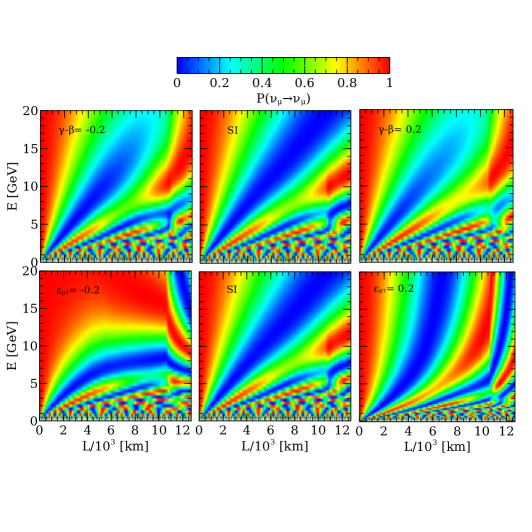
Figure 13: Oscillogram of $\nu_{\mu}\rightarrow\nu_{\mu}$ survival probability as a function of baseline $L$ and energy $E$. Top and bottom rows correspond to the oscillogram in presence of NSI parameter $(\gamma-\beta)$ and $\varepsilon_{\mu\tau}$, respectively. The middle column in both the rows shows the SI case. The first (third) column depicts the presence of negative (positive) NSI with a strength of 0.2. Values of the oscillation parameters are taken from Table 2. We assume $\theta_{23}=45^{\circ}$ and NMO.

To find out whether these features remain intact even if we assume non-zero $\theta_{13}$ and finite $\Delta m^{2}_{21}$, in Fig. 13, we have plotted the $\nu_{\mu}\rightarrow\nu_{\mu}$ survival probability as a function of baseline (x-axis) and energy (y-axis) commonly known as oscillogram plot. We first consider the full three-flavor vacuum expression of $\nu_{\mu}\rightarrow\nu_{\mu}$ survival probability without any approximation Agarwalla:2013tza and replace the vacuum parameters with their modified expressions in matter with NSI which we have derived in this work. As before, $\theta_{23}$ in vacuum is assumed to be $45^{\circ}$. In the top row, we compare the survival probabilities in presence of the parameter $(\gamma-\beta)$ with negative (left column) and positive (right column) values and compare with the SI case (middle column). We see that there is not any notable variation in oscillation pattern except for the magnitude of the survival probability, which decreases at high energies ($E$) and baselines ($L$). Some small differences in the pattern appear at some ($L,E$) region. It appears due to non-zero $\theta_{13}$ which brings the matter effect into the picture and the finite value of $\Delta_{21}$ which gives correction due to solar term. As predicted from Eq. 52, the sign of $(\gamma-\beta)$ does not affect the $\nu_{\mu}\rightarrow\nu_{\mu}$ disappearance probability.

In the bottom row of Fig. 13, we plot the same but in presence of $\varepsilon_{\mu\tau}$ with negative (positive) value in the extreme left (right) panel and show the results for SI case in the middle column. It is observed that the presence of $\varepsilon_{\mu\tau}$ can lead to significant differences in the pattern of $\nu_{\mu}\rightarrow\nu_{\mu}$ disappearance probability as compared to SI case. When $\varepsilon_{\mu\tau}$ is positive (negative), one can observe a significant shift in the oscillation dip (blue regions emerging from the origin) from the SI case towards higher (lower) energies in Fig. 13. This feature can be explained from the approximate expression in Eq. 52. In that expression, the value of $P^{m}_{\nu_{\mu}\rightarrow\nu_{\mu}}$ is mainly determined by the first term in R.H.S. since second term is suppressed by the NSI parameters appearing quadratically. At the first term in R.H.S. of Eq. 52, minimum occurs at higher (lower) energy compared to SI case for a given baseline $L$ when $\varepsilon_{\mu\tau}$ is present with positive (negative) strength. Depending on the sign of $\varepsilon_{\mu\tau}$, the regions representing the oscillation dip tend to bend upward or downward with increase in baseline length compared to SI case.

9 Summary and Concluding Remarks

In this work, we derive the expressions for the evolution of the fundamental mass-mixing parameters in the presence of SI and SI+NSI considering all possible lepton-flavor-conserving and lepton-favor-violating NC-NSI. In order to derive these expressions, we use a method of approximate diagonalization of the effective Hamiltonian by performing successive rotations in (2,3), (1,3), and (1,2) blocks. In our study, we present the results for the benchmark value of the DUNE baseline of 1300 km and also discuss the results for few other baselines. We consider both positive and negative values of real NSI parameters with benchmark values of $\pm~{}0.2$.

In the presence of SI only, the 2-3 mixing angle in matter ($\theta_{23}^{m}$) receives a tiny correction which is independent of energy and the strength of the matter potential. It is observed that only the NSI parameters in the (2,3) block, namely $\varepsilon_{\mu\tau}$ and $(\gamma-\beta)\equiv(\varepsilon_{\tau\tau}-\varepsilon_{\mu\mu})$ influence the evolution of $\theta_{23}^{m}$. In the presence of negative (positive) value of $(\gamma-\beta$), $\theta_{23}^{m}$ increases (decreases) with energy. For the maximal value of $\theta_{23}$ in vacuum, the change in $\theta_{23}^{m}$ is negligible in the presence of $\varepsilon_{\mu\tau}$. If $\theta_{23}$ belongs to the upper octant then $\theta_{23}^{m}$ increases (decreases) for negative (positive) choices of $\varepsilon_{\mu\tau}$. We notice a completely opposite behavior if $\theta_{23}$ lies in the lower octant. We also study the modification in $\theta_{23}^{m}$ as a function of energy when both the NSI parameters $\varepsilon_{\mu\tau}$ and $(\gamma-\beta)$ are present in the scenario with their all possible sign combinations. We unravel interesting degeneracies in $[\theta_{23}$ - $(\gamma-\beta)]$ and $[\theta_{23}$ - $\varepsilon_{\mu\tau}]$ planes for three different combination of $L$ and $E$ and discuss how our simple approximate analytical expression showing the evolution of $\theta_{23}^{m}$ plays an important role to understand these complicated degeneracy patterns.

In contrast to $\theta_{23}^{m}$, $\theta_{13}^{m}$ is more sensitive in matter in the presence of SI and SI+NSI. Therefore, an accurate understanding of the running of $\theta_{13}$ in matter is crucial to correctly assess the outcome of the oscillation experiments in the presence of NC-NSI. $\theta_{13}^{m}$ goes through an appreciable change even in SI case depending on the choice of mass ordering and whether we are dealing with neutrinos or antineutrinos. Compared to SI case, the relative change in $\theta_{13}^{m}$ for ($\nu$, NMO) is somewhat suppressed (enhanced) in the presence of positive (negative) NSI parameters in the (2,3) block, namely $\gamma\equiv(\varepsilon_{\tau\tau}-\varepsilon_{ee})$, $\beta\equiv(\varepsilon_{\mu\mu}-\varepsilon_{ee})$, and $\varepsilon_{\mu\tau}$. For positive $\varepsilon_{e\mu}$ and/or $\varepsilon_{e\tau}$, $\theta_{13}^{m}$ for ($\nu$, NMO) approaches the resonance ($\theta_{13}^{m}=45^{\circ}$) faster than SI case, but after crossing the resonance energy, SI takes over. For negative $\varepsilon_{e\mu}$ or $\varepsilon_{e\tau}$, running of $\theta_{13}^{m}$ is suppressed almost up to the resonance energy and then, it increases very steeply compared to SI case.

As far as the solar mixing angle is concerned, $\theta_{12}^{m}$ approaches to $90^{\circ}$ ($\sin\theta_{12}^{m}\to 1$, $\cos\theta_{12}^{m}\to 0$) very quickly as we increase the neutrino energy in SI case. While the NSI parameters in the (2,3) block ($\gamma,\beta,\varepsilon_{\mu\tau}$) have minimal impact on the running of $\theta_{12}^{m}$, $\varepsilon_{e\mu}$ and $\varepsilon_{e\tau}$ affect the evolution of $\theta_{12}^{m}$ substantially. In the presence of positive (negative) $\varepsilon_{e\mu}$, the change in $\theta_{12}^{m}$ with energy qualitatively remains the same with the saturation value turns out to be around $80^{\circ}$ ($100^{\circ}$). In the presence of positive (negative) $\varepsilon_{e\tau}$, the saturation happens around $100^{\circ}$ ($80^{\circ}$).

Out of the two mass-squared differences, the evolution of the solar $\Delta m^{2}_{21,m}$ is quite dramatic as compared to that of the atmospheric $\Delta m^{2}_{31,m}$ in matter. Both in SI and SI+NSI cases, as we increase the energy and go beyond 10 GeV, the value of $\Delta m^{2}_{21,m}$ increases to almost 20 times as compared to its vacuum value for 1300 km baseline. At the same time, the value of $\Delta m^{2}_{31,m}$ does not change much compared to its vacuum value.

We demonstrate the utility of our approach in addressing some interesting features that we observe in neutrino oscillation in presence of matter. It is well known that $\theta_{13}^{m}$ can attain the value of $45^{\circ}$ (MSW-resonance condition) for some choices of $L$ and $E$ in the presence of standard matter effect. Now, in this work, for the first time, we show how the $\theta_{13}$-resonance energy gets modified in the presence of NC-NSI with the help of simple, compact, approximate analytical expressions. We observe that only the NSI parameters in the $(2,3)$ block affects the $\theta_{13}$-resonance energy.

We study in detail how the NC-NSI parameters affect $\nu_{\mu}\rightarrow\nu_{e}$ oscillation probability which plays an important role to address the remaining unknown issues, namely CP violation, mass ordering, and the precision measurement of oscillation parameters. In this paper, for the first time, we derive a simple approximate analytical expression for $E$, $L$ and its corresponding $\rho_{\text{avg}}$ to have the maximal matter effect which in turn gives rise to maximum $\nu_{\mu}\rightarrow\nu_{e}$ transition in the presence of all possible NC-NSI parameters. This analytical expression reveals that in SI case, maximum $\nu_{\mu}\rightarrow\nu_{e}$ transition occurs around the baselines almost passing through the core of the Earth ($\simeq$ 10600 km) under the assumption that the $\theta_{13}$-resonance energy coincides with the energy that corresponds to the first oscillation maximum. However, in the presence of positive $\varepsilon_{e\mu}$ or $\varepsilon_{e\tau}$ in matter, it is observed that the baseline length for maximum $\nu_{\mu}\rightarrow\nu_{e}$ transition probability gets reduced to a much lower value ($L\approx$ 6700 km) for the benchmark choices of $\varepsilon_{e\mu}$ or $\varepsilon_{e\tau}$ equal to 0.2. On the other hand, if we consider negative $\varepsilon_{e\mu}$ or $\varepsilon_{e\tau}$, the required baseline for maximum transition probability increases to a value that exceeds the diameter of the Earth.

We also study in detail how the NSI parameters in the (2,3) block affect $\nu_{\mu}\to\nu_{\mu}$ disappearance channel which plays an important role in atmospheric neutrino experiments. We observe that the off-diagonal NSI parameter $\varepsilon_{\mu\tau}$ has the dominant effect as compared to the diagonal NSI parameter $(\gamma-\beta)$. It happens because $(\gamma-\beta)$ appears in the second-order in the approximate $\nu_{\mu}\rightarrow\nu_{\mu}$ oscillation probability expression, whereas $\varepsilon_{\mu\tau}$ shows a liner dependence. Also, the sign of $\varepsilon_{\mu\tau}$ has a significant impact on $\nu_{\mu}\rightarrow\nu_{\mu}$ disappearance channel. However, this oscillation channel is not sensitive to the sign of the NSI parameter $(\gamma-\beta)$. We hope that the analysis performed in this paper will take our understanding of the evolution of the oscillation parameters in the presence of all possible NC-NSI a step forward.

Acknowledgments

We would like to thank T. Takeuchi, P. Denton, and E. Esteban for useful discussions. S.D. is grateful to the organizers of the Neutrino 2020 Online Conference at Fermilab, Chicago, USA during 22nd June to 2nd July, 2020 for giving an opportunity to present a poster based on this work. S.D. would also like to thank the organizers of the XXIV DAE-BRNS High Energy Physics Online Symposium at NISER, Bhubaneswar, India during 14th to 18th December, 2020 for providing him an opportunity to give a talk based on this study. We thank the Department of Atomic Energy (DAE), Govt. of India for financial support. S.K.A. is supported by the INSPIRE Faculty Research Grant [IFA-PH-12] from the Department of Science and Technology (DST), Govt. of India. S.K.A. acknowledges the financial support from the Swarnajayanti Fellowship Research Grant (No. DST/SJF/PSA-05/2019-20) provided by the DST, Govt. of India and the Research Grant (File no. SB/SJF/2020-21/21) from the Science and Engineering Research Board (SERB) under the Swarnajayanti Fellowship by the DST, Govt. of India. S.K.A. and M.M. acknowledge the financial support from the Indian National Science Academy (INSA) Young Scientist Project [INSA/SP/YS/2019/269]. M.M. acknowledges the support of IBS under the project code IBS-R018-D1.

References

- (1) Particle Data Group Collaboration, P. Zyla et al., Review of Particle Physics, PTEP 2020 (2020), no. 8 083C01.
- (2) Super-Kamiokande Collaboration, Y. Fukuda et al., Evidence for oscillation of atmospheric neutrinos, Phys. Rev. Lett. 81 (1998) 1562, [hep-ex/9807003].
- (3) A. Marrone, Phenomenology of Three Neutrino Oscillations, 2021. Talk given at the XIX International Workshop on Neutrino Telescopes, 18th to 26th February, 2021, Padova, Italy, https://agenda.infn.it/event/24250/overview.
- (4) NuFIT 5.0 (2020), http://www.nu-fit.org/.
- (5) I. Esteban, M. C. Gonzalez-Garcia, M. Maltoni, T. Schwetz, and A. Zhou, The fate of hints: updated global analysis of three-flavor neutrino oscillations, JHEP 09 (2020) 178, [arXiv:2007.14792].
- (6) P. F. de Salas, D. V. Forero, S. Gariazzo, P. Martínez-Miravé, O. Mena, C. A. Ternes, M. Tórtola, and J. W. F. Valle, 2020 global reassessment of the neutrino oscillation picture, JHEP 02 (2021) 071, [arXiv:2006.11237].
- (7) R. N. Mohapatra et al., Theory of neutrinos: A White paper, Rept. Prog. Phys. 70 (2007) 1757–1867, [hep-ph/0510213].
- (8) A. Strumia and F. Vissani, Neutrino masses and mixings and…, hep-ph/0606054.
- (9) M. C. Gonzalez-Garcia and M. Maltoni, Phenomenology with Massive Neutrinos, Phys. Rept. 460 (2008) 1–129, [arXiv:0704.1800].
- (10) Super-Kamiokande Collaboration, Y. Ashie et al., Evidence for an oscillatory signature in atmospheric neutrino oscillation, Phys. Rev. Lett. 93 (2004) 101801, [hep-ex/0404034].
- (11) IceCube Collaboration, M. G. Aartsen et al., Measurement of Atmospheric Neutrino Oscillations at 6–56 GeV with IceCube DeepCore, Phys. Rev. Lett. 120 (2018), no. 7 071801, [arXiv:1707.07081].
- (12) ANTARES Collaboration, A. Albert et al., Measuring the atmospheric neutrino oscillation parameters and constraining the 3+1 neutrino model with ten years of ANTARES data, JHEP 06 (2019) 113, [arXiv:1812.08650].
- (13) Daya Bay Collaboration, D. Adey et al., Measurement of the Electron Antineutrino Oscillation with 1958 Days of Operation at Daya Bay, Phys. Rev. Lett. 121 (2018), no. 24 241805, [arXiv:1809.02261].
- (14) RENO Collaboration, J. Ahn et al., Observation of Reactor Electron Antineutrino Disappearance in the RENO Experiment, Phys. Rev. Lett. 108 (2012) 191802, [arXiv:1204.0626].
- (15) T2K Collaboration, K. Abe et al., Constraint on the matter–antimatter symmetry-violating phase in neutrino oscillations, Nature 580 (2020), no. 7803 339–344, [arXiv:1910.03887]. [Erratum: Nature 583, E16 (2020)].
- (16) T2K Collaboration, K. Abe et al., Improved constraints on neutrino mixing from the T2K experiment with protons on target, arXiv:2101.03779.
- (17) NOvA Collaboration, M. Acero et al., First Measurement of Neutrino Oscillation Parameters using Neutrinos and Antineutrinos by NOvA, Phys. Rev. Lett. 123 (2019), no. 15 151803, [arXiv:1906.04907].
- (18) DUNE Collaboration, B. Abi et al., Deep Underground Neutrino Experiment (DUNE), Far Detector Technical Design Report, Volume II DUNE Physics, arXiv:2002.03005.
- (19) DUNE Collaboration, B. Abi et al., Experiment Simulation Configurations Approximating DUNE TDR, arXiv:2103.04797.
- (20) Hyper-Kamiokande Proto-Collaboration Collaboration, K. Abe et al., Physics potential of a long-baseline neutrino oscillation experiment using a J-PARC neutrino beam and Hyper-Kamiokande, PTEP 2015 (2015) 053C02, [arXiv:1502.05199].
- (21) Hyper-Kamiokande Collaboration, K. Abe et al., Physics potentials with the second Hyper-Kamiokande detector in Korea, PTEP 2018 (2018), no. 6 063C01, [arXiv:1611.06118].
- (22) ESSnuSB Collaboration, E. Baussan et al., A very intense neutrino super beam experiment for leptonic CP violation discovery based on the European spallation source linac, Nucl. Phys. B 885 (2014) 127–149, [arXiv:1309.7022].
- (23) M. M. Devi, T. Thakore, S. K. Agarwalla, and A. Dighe, Enhancing sensitivity to neutrino parameters at INO combining muon and hadron information, JHEP 10 (2014) 189, [arXiv:1406.3689].
- (24) ICAL Collaboration, S. Ahmed et al., Physics Potential of the ICAL detector at the India-based Neutrino Observatory (INO), Pramana 88 (2017), no. 5 79, [arXiv:1505.07380].
- (25) A. Kumar, A. Khatun, S. K. Agarwalla, and A. Dighe, From oscillation dip to oscillation valley in atmospheric neutrino experiments, Eur. Phys. J. C 81 (2021), no. 2 190, [arXiv:2006.14529].
- (26) JUNO Collaboration, F. An et al., Neutrino Physics with JUNO, J. Phys. G 43 (2016), no. 3 030401, [arXiv:1507.05613].
- (27) Theia Collaboration, M. Askins et al., THEIA: an advanced optical neutrino detector, Eur. Phys. J. C80 (2020), no. 5 416, [arXiv:1911.03501].
- (28) C. A. Argüelles et al., New opportunities at the next-generation neutrino experiments I: BSM neutrino physics and dark matter, Rept. Prog. Phys. 83 (2020), no. 12 124201, [arXiv:1907.08311].
- (29) S. K. Agarwalla, BSM Searches in Neutrino Experiments, 2020. Talk given at the XXIX International Conference on Neutrino Physics and Astrophysics (Neutrino 2020), 22nd June to 2nd July, Fermilab, Chicago, USA, https://conferences.fnal.gov/nu2020/.
- (30) L. Wolfenstein, Neutrino Oscillations in Matter, Phys. Rev. D17 (1978) 2369–2374.
- (31) J. Valle, Resonant Oscillations of Massless Neutrinos in Matter, Phys. Lett. B 199 (1987) 432–436.
- (32) M. Guzzo, A. Masiero, and S. Petcov, On the MSW effect with massless neutrinos and no mixing in the vacuum, Phys. Lett. B 260 (1991) 154–160.
- (33) E. Roulet, MSW effect with flavor changing neutrino interactions, Phys. Rev. D 44 (1991) 935–938.
- (34) Y. Grossman, Nonstandard neutrino interactions and neutrino oscillation experiments, Phys. Lett. B 359 (1995) 141–147, [hep-ph/9507344].
- (35) M. M. Guzzo, H. Nunokawa, P. C. de Holanda, and O. L. G. Peres, On the massless ’just-so’ solution to the solar neutrino problem, Phys. Rev. D 64 (2001) 097301, [hep-ph/0012089].
- (36) P. Huber and J. W. F. Valle, Nonstandard interactions: Atmospheric versus neutrino factory experiments, Phys. Lett. B 523 (2001) 151–160, [hep-ph/0108193].
- (37) A. M. Gago, M. M. Guzzo, P. C. de Holanda, H. Nunokawa, O. L. G. Peres, V. Pleitez, and R. Zukanovich Funchal, Global analysis of the postSNO solar neutrino data for standard and nonstandard oscillation mechanisms, Phys. Rev. D 65 (2002) 073012, [hep-ph/0112060].
- (38) F. J. Escrihuela, M. Tortola, J. W. F. Valle, and O. G. Miranda, Global constraints on muon-neutrino non-standard interactions, Phys. Rev. D 83 (2011) 093002, [arXiv:1103.1366].
- (39) M. Gonzalez-Garcia, M. Maltoni, and J. Salvado, Testing matter effects in propagation of atmospheric and long-baseline neutrinos, JHEP 05 (2011) 075, [arXiv:1103.4365].
- (40) T. Ohlsson, Status of non-standard neutrino interactions, Rept. Prog. Phys. 76 (2013) 044201, [arXiv:1209.2710].
- (41) M. C. Gonzalez-Garcia and M. Maltoni, Determination of matter potential from global analysis of neutrino oscillation data, JHEP 09 (2013) 152, [arXiv:1307.3092].
- (42) O. G. Miranda and H. Nunokawa, Non standard neutrino interactions: current status and future prospects, New J. Phys. 17 (2015), no. 9 095002, [arXiv:1505.06254].
- (43) Y. Farzan and M. Tortola, Neutrino oscillations and Non-Standard Interactions, Front. in Phys. 6 (2018) 10, [arXiv:1710.09360].
- (44) A. Khatun, S. S. Chatterjee, T. Thakore, and S. Kumar Agarwalla, Enhancing sensitivity to non-standard neutrino interactions at INO combining muon and hadron information, Eur. Phys. J. C 80 (2020), no. 6 533, [arXiv:1907.02027].
- (45) Neutrino Non-Standard Interactions: A Status Report, vol. 2, 2019.
- (46) A. Kumar, A. Khatun, S. K. Agarwalla, and A. Dighe, A New Approach to Probe Non-Standard Interactions in Atmospheric Neutrino Experiments, arXiv:2101.02607.
- (47) S. P. Mikheyev and A. Yu. Smirnov, Resonance Amplification of Oscillations in Matter and Spectroscopy of Solar Neutrinos, Sov. J. Nucl. Phys. 42 (1985) 913–917.
- (48) S. P. Mikheev and A. Yu. Smirnov, Resonant amplification of neutrino oscillations in matter and solar neutrino spectroscopy, Nuovo Cim. C9 (1986) 17–26.
- (49) G. Barenboim, P. B. Denton, S. J. Parke, and C. A. Ternes, Neutrino Oscillation Probabilities through the Looking Glass, Phys. Lett. B 791 (2019) 351–360, [arXiv:1902.00517].
- (50) S. T. Petcov and S. Toshev, Three Neutrino Oscillations in Matter: Analytical Results in the Adiabatic Approximation, Phys. Lett. B 187 (1987) 120–126.
- (51) C. W. Kim and W. K. Sze, Adiabatic Resonant Oscillations of Solar Neutrinos in Three Generations, Phys. Rev. D 35 (1987) 1404.
- (52) J. Arafune and J. Sato, CP and T violation test in neutrino oscillation, Phys. Rev. D 55 (1997) 1653–1658, [hep-ph/9607437].
- (53) J. Arafune, M. Koike, and J. Sato, CP violation and matter effect in long baseline neutrino oscillation experiments, Phys. Rev. D 56 (1997) 3093–3099, [hep-ph/9703351]. [Erratum: Phys.Rev.D 60, 119905 (1999)].
- (54) T. Ohlsson and H. Snellman, Three flavor neutrino oscillations in matter, J. Math. Phys. 41 (2000) 2768–2788, [hep-ph/9910546]. [Erratum: J.Math.Phys. 42, 2345 (2001)].
- (55) M. Freund, Analytic approximations for three neutrino oscillation parameters and probabilities in matter, Phys. Rev. D 64 (2001) 053003, [hep-ph/0103300].
- (56) A. Cervera, A. Donini, M. Gavela, J. Gomez Cadenas, P. Hernandez, O. Mena, and S. Rigolin, Golden measurements at a neutrino factory, Nucl. Phys. B 579 (2000) 17–55, [hep-ph/0002108]. [Erratum: Nucl.Phys.B 593, 731–732 (2001)].
- (57) E. K. Akhmedov, R. Johansson, M. Lindner, T. Ohlsson, and T. Schwetz, Series expansions for three flavor neutrino oscillation probabilities in matter, JHEP 04 (2004) 078, [hep-ph/0402175].
- (58) K. Asano and H. Minakata, Large-Theta(13) Perturbation Theory of Neutrino Oscillation for Long-Baseline Experiments, JHEP 06 (2011) 022, [arXiv:1103.4387].
- (59) S. K. Agarwalla, Y. Kao, and T. Takeuchi, Analytical approximation of the neutrino oscillation matter effects at large , JHEP 04 (2014) 047, [arXiv:1302.6773].
- (60) H. Minakata and S. J. Parke, Simple and Compact Expressions for Neutrino Oscillation Probabilities in Matter, JHEP 01 (2016) 180, [arXiv:1505.01826].
- (61) P. B. Denton, H. Minakata, and S. J. Parke, Compact Perturbative Expressions For Neutrino Oscillations in Matter, JHEP 06 (2016) 051, [arXiv:1604.08167].
- (62) M. Gonzalez-Garcia, Y. Grossman, A. Gusso, and Y. Nir, New CP violation in neutrino oscillations, Phys. Rev. D 64 (2001) 096006, [hep-ph/0105159].
- (63) T. Ota, J. Sato, and N.-a. Yamashita, Oscillation enhanced search for new interaction with neutrinos, Phys. Rev. D 65 (2002) 093015, [hep-ph/0112329].
- (64) O. Yasuda, On the exact formula for neutrino oscillation probability by Kimura, Takamura and Yokomakura, arXiv:0704.1531.
- (65) J. Kopp, M. Lindner, T. Ota, and J. Sato, Non-standard neutrino interactions in reactor and superbeam experiments, Phys. Rev. D 77 (2008) 013007, [arXiv:0708.0152].
- (66) N. C. Ribeiro, H. Minakata, H. Nunokawa, S. Uchinami, and R. Zukanovich-Funchal, Probing Non-Standard Neutrino Interactions with Neutrino Factories, JHEP 12 (2007) 002, [arXiv:0709.1980].
- (67) M. Blennow and T. Ohlsson, Approximative two-flavor framework for neutrino oscillations with non-standard interactions, Phys. Rev. D 78 (2008) 093002, [arXiv:0805.2301].
- (68) T. Kikuchi, H. Minakata, and S. Uchinami, Perturbation Theory of Neutrino Oscillation with Nonstandard Neutrino Interactions, JHEP 03 (2009) 114, [arXiv:0809.3312].
- (69) D. Meloni, T. Ohlsson, and H. Zhang, Exact and Approximate Formulas for Neutrino Mixing and Oscillations with Non-Standard Interactions, JHEP 04 (2009) 033, [arXiv:0901.1784].
- (70) S. K. Agarwalla, Y. Kao, D. Saha, and T. Takeuchi, Running of Oscillation Parameters in Matter with Flavor-Diagonal Non-Standard Interactions of the Neutrino, JHEP 11 (2015) 035, [arXiv:1506.08464].
- (71) V. D. Barger, K. Whisnant, S. Pakvasa, and R. J. N. Phillips, Matter Effects on Three-Neutrino Oscillations, Phys. Rev. D 22 (1980) 2718.
- (72) H. Zaglauer and K. Schwarzer, The Mixing Angles in Matter for Three Generations of Neutrinos and the Msw Mechanism, Z. Phys. C 40 (1988) 273.
- (73) T. Ohlsson and H. Snellman, Neutrino oscillations with three flavors in matter: Applications to neutrinos traversing the Earth, Phys. Lett. B 474 (2000) 153–162, [hep-ph/9912295]. [Erratum: Phys.Lett.B 480, 419–419 (2000)].
- (74) K. Kimura, A. Takamura, and H. Yokomakura, Exact formula of probability and CP violation for neutrino oscillations in matter, Phys. Lett. B 537 (2002) 86–94, [hep-ph/0203099].
- (75) K. Kimura, A. Takamura, and H. Yokomakura, Exact formulas and simple CP dependence of neutrino oscillation probabilities in matter with constant density, Phys. Rev. D 66 (2002) 073005, [hep-ph/0205295].
- (76) C. Jarlskog, Commutator of the Quark Mass Matrices in the Standard Electroweak Model and a Measure of Maximal CP Violation, Phys. Rev. Lett. 55 (1985) 1039.
- (77) V. A. Naumov, Three neutrino oscillations in matter, CP violation and topological phases, Int. J. Mod. Phys. D 1 (1992) 379–399.
- (78) P. Harrison and W. Scott, CP and T violation in neutrino oscillations and invariance of Jarlskog’s determinant to matter effects, Phys. Lett. B 476 (2000) 349–355, [hep-ph/9912435].
- (79) C. G. J. Jacobi, Uber ein leichtes Verfahren, die in der Theorie der Säkularstörangenvorkommenden Gleichungen numerisch Aufzuloösen, Crelle’s Journal 30 (1846) 51–94.
- (80) L. Wolfenstein, Neutrino Oscillations and Stellar Collapse, Phys. Rev. D 20 (1979) 2634–2635.
- (81) S.-F. Ge and S. J. Parke, Scalar Nonstandard Interactions in Neutrino Oscillation, Phys. Rev. Lett. 122 (2019), no. 21 211801, [arXiv:1812.08376].
- (82) D. Aristizabal Sierra, V. De Romeri, and N. Rojas, COHERENT analysis of neutrino generalized interactions, Phys. Rev. D 98 (2018) 075018, [arXiv:1806.07424].
- (83) J. Heeck and W. Rodejohann, Gauged L_mu - L_tau Symmetry at the Electroweak Scale, Phys. Rev. D 84 (2011) 075007, [arXiv:1107.5238].
- (84) Y. Farzan and I. M. Shoemaker, Lepton Flavor Violating Non-Standard Interactions via Light Mediators, JHEP 07 (2016) 033, [arXiv:1512.09147].
- (85) Y. Farzan and J. Heeck, Neutrinophilic nonstandard interactions, Phys. Rev. D 94 (2016), no. 5 053010, [arXiv:1607.07616].
- (86) K. Babu, A. Friedland, P. Machado, and I. Mocioiu, Flavor Gauge Models Below the Fermi Scale, JHEP 12 (2017) 096, [arXiv:1705.01822].
- (87) M. B. Wise and Y. Zhang, Lepton Flavorful Fifth Force and Depth-dependent Neutrino Matter Interactions, JHEP 06 (2018) 053, [arXiv:1803.00591].
- (88) H. Minakata, Probing Non-Standard Neutrino Physics at Neutrino Factory and T2KK, in 4th International Workshop on Neutrino Oscillations in Venice: Ten Years after the Neutrino Oscillations, pp. 361–380, 5, 2008. arXiv:0805.2435.
- (89) B. Pontecorvo, Inverse beta processes and nonconservation of lepton charge, Sov. Phys. JETP 7 (1958) 172–173.
- (90) Z. Maki, M. Nakagawa, and S. Sakata, Remarks on the unified model of elementary particles, Prog.Theor.Phys. 28 (1962) 870–880.
- (91) B. Pontecorvo, Neutrino Experiments and the Problem of Conservation of Leptonic Charge, Sov.Phys.JETP 26 (1968) 984–988.
- (92) I. Esteban, M. Gonzalez-Garcia, M. Maltoni, I. Martinez-Soler, and J. Salvado, Updated Constraints on Non-Standard Interactions from Global Analysis of Oscillation Data, JHEP 08 (2018) 180, [arXiv:1805.04530].
- (93) S. S. Chatterjee, A. Dasgupta, and S. K. Agarwalla, Exploring Flavor-Dependent Long-Range Forces in Long-Baseline Neutrino Oscillation Experiments, JHEP 12 (2015) 167, [arXiv:1509.03517].
- (94) A. M. Dziewonski and D. L. Anderson, Preliminary reference earth model, Phys. Earth Planet. Interiors 25 (1981) 297–356.
- (95) P. Huber, M. Lindner, and W. Winter, Simulation of long-baseline neutrino oscillation experiments with GLoBES (General Long Baseline Experiment Simulator), Comput. Phys. Commun. 167 (2005) 195, [hep-ph/0407333].
- (96) P. Huber, J. Kopp, M. Lindner, M. Rolinec, and W. Winter, New features in the simulation of neutrino oscillation experiments with GLoBES 3.0: General Long Baseline Experiment Simulator, Comput. Phys. Commun. 177 (2007) 432–438, [hep-ph/0701187].
- (97) M. C. Banuls, G. Barenboim, and J. Bernabeu, Medium effects for terrestrial and atmospheric neutrino oscillations, Phys. Lett. B 513 (2001) 391–400, [hep-ph/0102184].
- (98) R. Gandhi, P. Ghoshal, S. Goswami, P. Mehta, and S. Sankar, Large matter effects in oscillations, Phys. Rev. Lett. 94 (2005) 051801, [hep-ph/0408361].
- (99) R. Gandhi, P. Ghoshal, S. Goswami, P. Mehta, and S. U. Sankar, Earth matter effects at very long baselines and the neutrino mass hierarchy, Phys. Rev. D 73 (2006) 053001, [hep-ph/0411252].
- (100) J. Kopp and M. Lindner, Detecting atmospheric neutrino oscillations in the ATLAS detector at CERN, Phys. Rev. D 76 (2007) 093003, [arXiv:0705.2595].
- (101) I. Mocioiu and W. Wright, Non-standard neutrino interactions in the – sector, Nucl. Phys. B 893 (2015) 376–390, [arXiv:1410.6193].
- (102) M. Gonzalez-Garcia and M. Maltoni, Atmospheric neutrino oscillations and new physics, Phys. Rev. D 70 (2004) 033010, [hep-ph/0404085].