A Framework for 3D Tracking of Frontal Dynamic Objects in Autonomous Cars

Abstract

Both recognition and 3D tracking of frontal dynamic objects are crucial problems in an autonomous vehicle, while depth estimation as an essential issue becomes a challenging problem using a monocular camera. Since both camera and objects are moving, the issue can be formed as a structure from motion (SFM) problem. In this paper, to elicit features from an image, the YOLOv3 approach is utilized beside an OpenCV tracker. Subsequently, to obtain the lateral and longitudinal distances, a nonlinear SFM model is considered alongside a state-dependent Riccati equation (SDRE) filter and a newly developed observation model. Additionally, a switching method in the form of switching estimation error covariance is proposed to enhance the robust performance of the SDRE filter. The stability analysis of the presented filter is conducted on a class of discrete nonlinear systems. Furthermore, the ultimate bound of estimation error caused by model uncertainties is analytically obtained to investigate the switching significance. Simulations are reported to validate the performance of the switched SDRE filter. Finally, real-time experiments are performed through a multi-thread framework implemented on a Jetson TX2 board, while radar data is used for the evaluation.

1 Introduction

3D tracking of frontal dynamic objects is highly lucrative to obtain rich information about the surrounding environment in an autonomous vehicle. Since the movement is in two directions, the main purpose is to obtain the lateral and longitudinal distances of the frontal dynamic objects while recognizing them, simultaneously. The depth, however, is not directly measurable by a single camera, due to the 3D projection, and therefore, it has to be estimated. Deep learning has been proved to be applicable to solve this issue. As reported in [1], a method based on deep fully convolutional residual networks may be used to formulate depth estimation as a pixel-wise classification task and the main concept is to discretize the continuous ground-truth depth into several bins and label them regarding their depth ranges. In [2], a deep convolutional neural field model is presented which may be used for depth estimation of general scenes without any extra information such as geometric priors. Furthermore, in [3] and [4], an unsupervised training approach is proposed that enables a CNN to estimate the depth, despite the absence of ground truth depth data. Even though these methods promise a depth map of both indoor and outdoor environments, their computational cost prevents to simply utilize them in real-time applications. Moreover, these approaches are appropriate for static scenes or when a dense depth map is needed [5]. In the application mentioned in this article, frontal dynamic objects are counted as a sparse depth map requirement with lateral distance estimation. To the best knowledge of the authors these two objectives are not addressed simultaneously in any of the presented approaches in the literature.

On the other hand, there are other approaches reported in the literature, which are based on obtaining structure from motion. In these methods, movements are used to estimate the depth  [6, 7]. Basically, an SFM problem can be solved via deep learning techniques or classic methods. As the state-of-the-art deep learning based solution, [8] may be mentioned which proposes a physical driven architecture regardless of the accurate camera poses. This contains two cost volume based architectures for depth and pose estimation. The second representative approach is [9] which is based on robust image retrieval for coarse camera pose estimation and robust local features for accurate pose refinement. Deep learning based methods such as this approach solve the SFM problem through obtaining a dense depth map or a dense 3D map while the focus of this paper is on estimating of the longitudinal and lateral distances to specific frontal objects, which may be seen as producing a sparse map. Classic approaches, however, are more relevant taking an observer along with a model that relates the observations of feature points in a 2D image to the corresponding Euclidean coordinates in the inertia frame [10, 11, 12]. To be more specific, consider a moving object Euclidean position is needed and a single moving camera is utilized to obtain it. The first step is to determine feature points of the object and to take their positions as observations in the image. Then, a motion model together with an observer can be exploited to estimate both the longitudinal and lateral distances of the feature points. Regarding the second step, methods such as particle filter [13], variable structure [14], high-order sliding-mode [15], extended Kalman Filter (EKF) [16] and methods based on SDRE [17] may be considered.

To specify the feature points automatically, deep CNNs may be applied to detect and recognize the objects  [18, 19, 20]. There are diverse architectures that provide the capability to recognize visual patterns directly from pixel images with negligible preprocessing. For instance, AlexNet, ZFNet, ResNet, VGGNet, and YOLO are introduced with a different number of convolutional, pooling and fully connected layers for various applications [21]. Furthermore, OpenCV trackers [22] such as tracking-learning-detection (TLD) [23] and Median-flow [24] may be implemented alongside CNNs to reduce the computational cost.

2 Related Works and Motivation

To further clarify the gap in the literature and how this paprer has addressed it, consider two main components in solving an SFM problem in a real-world application. For the first component, consider a classic nonlinear observer that is employed to estimate the state variables while using the environmental observations. To produce the observations, however, it is necessary to take a strong image processing algorithm as the second component when utilizing a camera as the sensor. In the first component, several methods are proposed among which the unknown input observer (UIO) may be considered as the state-of-the-art (SOTA) since it is widely used in the estimation problems where unknown inputs such as disturbances are present [25, 26, 27]. In an SFM problem, the intended object velocities are taken as unknown inputs which makes the UIO a beneficial approach [10, 28]. This observer basically eliminates the unknown input effects and is commonly used in the literature for various applications [29, 30]. The main assumption in employing a UIO approach is, however, to have a perfect model of the system which indeed is a limiting hypothesis. Thus, the first contribution of this paper is to propose a new discrete-time nonlinear observer to address the SFM problem in presence of model uncertainties. A comparison study is performed with respect to the UIO to reveal the capability of the presented estimator. According to the reported results, the UIO performs better when the model is perfect; however, the proposed nonlinear observer outperforms the UIO in the presence of modeling uncertainty. Besides, the SFM problem is not applicable to the autonomous vehicle field since it needs the movement of the camera in all the three directions based on some basic assumptions [10, 11]. In this regard, a new observation model is necessary to be added to the SFM problem to further generalize this approach to the autonomous vehicle area. Giving attention to the second component, almost all of the presented approaches employ a simple method to produce the observations such as utilizing a pre-mounted marker on the target or considering specific target features while focusing on the first component of the problem [11, 28, 29]. This, of course, is not applicable to the problem of estimating the distances to the frontal objects about which there is no a priori-knowledge. Consequently, a real-time image processing method is necessary to produce the observations robustly. Finally, all the previous approaches are presented to estimate the variables for short distances. This research, however, covers estimation of the lateral and longitudinal distances up to $80$ meters away from the host vehicle which is crucial in case of an autonomous vehicle application.
The SFM problem addressed in this paper includes the estimation of all the coordinates corresponding to a feature point. However, in the machine learning field, especially in the deep learning methods, the simplified problem of just estimating the depth is taken into consideration. In [31], it has been claimed that the first end-to-end learning-based model is developed to directly predict distances for given objects in the images. The mentioned research is associated with only the depth estimation, in the absense of lateral distance prediction. Furthermore, as the stringent requirement for this CNN model the object bounding boxes are needed, which in turns requires adding another deep CNN like YOLO, and thus downgrading its performance. The other similar work is presented in [32], where an RCNN [33] based architecture is used as the main model along with another shallow network to accomplish the task of the detection and distance estimation, simultaneously. Comparing this approach with the one presented in this paper, obviously, the RCNN architecture yields poor performance in terms of computation cost and execution speed, while the lateral distance is not considered at all. Finally, as a powerful approach, [34] proposes DisNet to estimate the depth up to $100$ meters while its accuracy reaches to $90\%$. It uses a deep neural network consisting of three hidden layers with $100$ neurons at each layer, while it is just evaluated on a number of specific static scenes, and not considering the lateral distance like other mentioned approaches. As a result, it can be remarked that this is the first time that the problem of both the lateral and longitudinal distances estimation is formulated and worked out for dynamic environment.

In this paper, a rigid body kinematic motion model as exploited in [11] is used alongside YOLOv3 [35], Median-flow tracker and a newly designed filter to estimate the longitudinal and the lateral distances of frontal objects. Since the dynamics of these two variables are not linear, nonlinear filters are preferable. SDRE filter high degree of freedom provides singularity avoidance making it a proper choice employed in various applications as the optimal solution for nonlinear estimation and control problems [36, 37, 38]. This filter incorporates the nonlinearity into the estimation equations based on a parameterization which compared to the EKF is counted as a significant advantage since the EKF linearizes the nonlinearity [39]. However, model uncertainty yields limitations in the SDRE filter implementation which can be further empowered based on a switching concept presented in this research. Consequently, a discrete time-dependent switching-based SDRE filter is proposed, to further improve the structural robustness of the common SDRE filter against model uncertainty. More accurately, incorporation of switching concepts and traditional SDRE filter increases the SDRE filter performance in the presence of uncertainties. It is worth noting that in this approach, the switching of estimation error covariance matrix with a predetermined frequency is considered in the filter dynamics. The main outcome of the proposed method is regulation of estimation error covariance matrix eigenvalues which result in more robustness and a lower amount of ultimate error bound. Note that, the concept of using switching is presented in the author’s previous research [40] for continuous-time systems. In this paper, the proposed estimator is extended to the discrete-time systems, while it is applied to the application of autonomous cars. The literature regarding the stability analysis and the equations of the estimator is far different of that of the continous-time. The theorems along with the lemmas derived in this article can be used in further theoretical developments in discrete-time related approaches. Considering the application of the proposed filter in estimation theory, stability analysis based on the Lyapunov theorem is performed on a class of nonlinear systems. Then robustness analysis is accomplished and the influence of switching on the ultimate bound of estimation error is investigated. Simulations are given to reveal the effectiveness of the proposed filter, and finally, real-time implementation results of the filter are reported to verify the theoretical developments in the application of autonomous vehicles.

The rest of this paper is arranged as follows. In section II the mathematical preliminaries are presented along with stability analysis of the proposed filter and ultimate error bound determination. Section III concentrates on the model utilized to estimate both longitudinal and lateral positions of frontal dynamic objects. In section IV, simulations are performed on the comparison of the proposed filter with other methods on solving the SFM problem. Experimental results are reported in section V to verify the applicability of the proposed approach. Finally, concluding remarks are presented in section VI.

3 The Designed Filter Theory

3.1 Preliminaries

Assume the general representation of a nonlinear system as follows.

$$x(t+1)=f(x(t),u(t))+\Delta f(x(t),u(t))+Gw_{0}(t)$$ (1)

$$y(t)=h(x(t),u(t))+\Delta h(x(t),u(t))+D_{1}v_{0}(t)$$ (2)

where $x(t)\in\Re^{n}$ represents the system state vector, $u(t)\in\Re^{m}$ is the input, $y(t)\in\Re^{p}$ indicates the observed output, $w_{0}(t)$ and $v_{0}(t)$, are the process and measurement noises with unknown statistical properties, respectively; furthermore, $\Delta f(x(t),u(t))$ and $\Delta h(x(t),u(t))$ are the model uncertainties. Note that, $t$ denotes the time-step.

SDRE method is based on a state dependent coefficient (SDC) formed state space. According to [41], most non-linear state equations can be transformed to this form. Thus, rewriting the system model in SDC form yields:

$$x(t+1)=A(x(t))x(t)+\Delta f(x(t))+B(x(t))u(t)$$

$$+\Delta B(x(t))u(t)+Gw_{0}(t)$$ (3)

$$y(t)=C(x(t))x(t)+\Delta h(x(t))+D(x(t))u(t)$$

$$+\Delta D(x(t))u(t)+D_{1}v_{0}(t)$$ (4)

considering the following assumption holds : $\Delta f(x,u)=\Delta f(x)+\Delta B(x)u$ and $\Delta h(x,u)=\Delta h(x)+\Delta D(x)u$.

Remark 1: SDC form is not unique for multivariable systems as if $A_{1}(x)$ and $A_{2}(x)$ are two distinct factor coefficients of $f(x)$, then, $A_{3}(x)=Z(x)A_{1}(x)+(I-Z(x))A_{2}(x)$ is a parameterizations of $f(x)$ for any matrix function $Z(x)\in\Re^{n\times n}$ as well. This flexibility is valid for $A(x)$, $B(x)$, $C(x)$ and $D(x)$.

This Remark shows a significant advantage of SDRE method, which results in design process efficiency such as singular and unobservable points avoidance, and Lipschitz condition realization. The main objective is to design a filter which estimates the state vector $x(t)$ robustly, through measurable output vector, $y(t)$. The proposed filter equation is presented as follows.

$$\hat{x}(t+1)=A(\hat{x})\hat{x}(t)+B(\hat{x})u(t)$$

$$+L(\hat{x},t)[y(t)-(C(\hat{x})\hat{x}(t)+D(\hat{x})u(t))]$$ (5)

where $\hat{x}(t)$ demonstrates estimated state variable vector and the filter gain $L(\hat{x},t)\in\Re^{n\times p}$, is defined as

$$L(\hat{x},t)=A(\hat{x})P(t)C^{T}(\hat{x})[C(\hat{x})P(t)C^{T}(\hat{x})+R(t)]^{-1}$$ (6)

in which, the symmetric matrix $P(t)\in\Re^{n\times n}$ satisfies the state dependent differential Riccati equation (SDDRE) (3.1) with positive definite matrices $Q(t)\in\Re^{n\times n}$ and $R\in\Re^{p\times p}$ [42].

$$P(t+1)=A(\hat{x})P(t)A^{T}(\hat{x})+Q-A(\hat{x})P(t)C^{T}(\hat{x})[$$

$$C(\hat{x})P(t)C^{T}(\hat{x})+R(t)]^{-1}C(\hat{x})P(t)A^{T}(\hat{x})$$ (7)

The estimation error is defined as following:

$$e(t)=x(t)-\hat{x}(t)$$ (8)

Subtract(3.1) from (3.1) and perform some simplifications to reach to:

$$e(t+1)=[A(\hat{x})-L(\hat{x},t)C(\hat{x})]e(t)+\alpha(x,\hat{x},u)$$

$$-L(\hat{x},t)\beta(x,\hat{x},u)-L(\hat{x},t)v(t)+\Gamma w(t)$$ (9)

where,

$$\alpha(x,\hat{x},u)=[A(x)-A(\hat{x})]x(t)+[B(x)-B(\hat{x})]u(t)$$ (10)

$$\beta(x,\hat{x},u)=[C(x)-C(\hat{x})]x(t)+[D(x)-D(\hat{x})]u(t)$$ (11)

and

$$w=(\Delta f(x)\quad\Delta B(x)u(t)\quad w_{0}(t))^{T},$$

$$\Gamma=(I\quad I\quad G),$$

$$v=(I\quad I\quad I)(\Delta h(x)\quad\Delta D(x)u(t)\quad D_{1}v_{0})^{T}.$$

As the final step to develop the proposed filter, the switching concept is incorporated. It is proposed to switch $P(t)$ to its initial value with a specific frequency that is obtained through estimation error stability and ultimate error bound analysis. As a result, the filter estimation is divided into a family of subsystems, that can be studied in switched systems domain.

3.2 Stability Analysis

In this subsection, the sufficient condition for the estimation error dynamic stability is obtained. Furthermore, the ultimate estimation error bound caused by the model uncertainties is analytically acquired to further investigate the switching effects. Since time dependent switching is applied, the following dwell-time theorem is proven here for the sake of stability analysis.

Theorem 1.

Consider the non-linear discrete-time system presented in equations (3.1) and (3.1), along with equations (3.1), (6) and (3.1), related to the proposed filter, and suppose the following assumptions hold:

1) There exist $\overline{a},\overline{c}>0$, which $A(x)$ and $C(x)$ are upper-bounded for any $k\geq 0$ as follows:

$$\|A(x)\|\leq\overline{a},\;\;\|C(x)\|\leq\overline{c}$$ (12)

2) The states and inputs are bounded such that

$$\|x(t)\|\leq\sigma,\;\;\|u(t)\|\leq\rho$$ (13)

where $\sigma,\rho>0$ for $t\geq 0$.

3) $P(t)$, the solution of Riccati differential equation is bounded as follows

$$\underline{p}I\leq P(t)\leq\overline{p}I$$ (14)

where $\overline{p}$, $\underline{p}$ are positive real numbers.

4) The SDC parameterizations is chosen such that matrices $A(x),B(x),C(x),D(x)$ are locally Lipschitz, i.e., there exist constants $k_{A},k_{B},k_{C},k_{D}>0$ such that

$$\|A(x)-A(\hat{x})\|\leq k_{A}\|x-\hat{x}\|$$ (15)

$$\|B(x)-B(\hat{x})\|\leq k_{B}\|x-\hat{x}\|$$ (16)

$$\|C(x)-C(\hat{x})\|\leq k_{C}\|x-\hat{x}\|$$ (17)

$$\|D(x)-D(\hat{x})\|\leq k_{D}\|x-\hat{x}\|$$ (18)

for any $x,\hat{x}\in\Re^{n}$ with $\|x-\hat{x}\|\leq\varepsilon_{A}$ and $\|x-\hat{x}\|\leq\varepsilon_{B}$ and $\|x-\hat{x}\|\leq\varepsilon_{C}$ and $\|x-\hat{x}\|\leq\varepsilon_{D}$, respectively.

Then, to have stable estimation error dynamic (3.1), the following condition is adequate to be hold for positive numbers $\kappa^{\prime}$ and $\lambda$.

$$2\kappa^{\prime}\|\Pi(t+1)[-L(\hat{x},t)v(t)+\Gamma w(t)]\|+(\lambda_{0}+\frac{\lambda}{2})\lambda_{max}^{\Pi(t)}\leq\lambda\lambda_{min}^{\Pi(t)}$$ (19)

where $\lambda_{0}$ is directly related to the switching frequency and $\Pi(t)=P^{-1}(t)$.

Remark 2: The maximum and minimum eigenvalues of $\Pi$ are represented by $\lambda_{max}^{\Pi}$ and $\lambda_{min}^{\Pi}$, respectively.

Before presenting the proof of theorem 1, some points have to be mentioned.

Remark 3: Inequality (14) is very important to be satisfied in estimation error stability. This is directly related to the system observability based on the following assumptions [43]:

1- The design matrix $Q$ and initial condition $P(0)$ are positive definite and $A(x)$ has a bounded norm.

2- The SDC form is chosen such that the pair of $\{A(x),C(x)\}$ is uniformly detectable through Definition 1.

Definition 1.

$\{A(x),C(x)\}$ satisfies the uniform observability condition, if there exist $\underline{m},\overline{m}>0$ and $a>0$ as an integer such that

$$\underline{m}I\leq\sum_{i=t}^{t+a}\chi^{-T}(i,t)C_{i}^{T}C_{i}\chi(i,t)\leq\overline{m}I$$ (20)

where $\chi(t,t)=I$ and for $i>t$ the following is valid

$$\chi(i,t)=A_{i-1}...A_{t}$$ (21)

Remark 4: Assumption 4 is commonly considered in researches [44] and compared to the previous SDRE filter studies, there is no new limiting condition for the mentioned SDC form.

Remark 5: Switching the covariance matrix yields to a family of subsystems which their stability can be analyzed by considering distinct Lyapunov functions for each subsystem based on direct Lyapunov method.

Proof.

Theorem 1 is proved within two steps through exploiting the following Lemma.

Lemma 1.

Consider (3.1) as a set of subsystems. Suppose there exist a Lyapunov candidate function $V_{p}$ for subsystem $p$ along with two $K_{\infty}$-class functions $\alpha_{1}$ and $\alpha_{2}$, and two constants $0<\lambda_{0}<1$ and $\mu>0$ such that

$$\alpha_{1}(\|x\|)\leq V_{p}(x)\leq\alpha_{2}(\|x\|)\quad\forall x,\quad\forall p\in\varrho$$ (22)

$$\Delta V_{p}(x)\leq-\lambda_{0}V_{p}(x)\quad\forall x,\quad\forall p\in\varrho$$ (23)

$$V_{p}(x)\leq\mu V_{q}(x)\quad\forall x,\quad\forall p,q\in\varrho$$ (24)

where, $\varrho$ denotes the set of all subsystems. Then, the non-linear discrete-time switched system (3.1) is stable for every switching signal with average dwell-time $\tau_{a}$ if

$$\tau_{a}>-\frac{\ln{\mu}}{\ln(1-\lambda_{0})}$$ (25)

Lemma1 is comprehensively studied along with its proof in [45]. Since inequality (22) holds due to assumption 3, the two following steps focus on ensuring conditions (23) and (24).

Step 1: To present the sufficient condition for (23), the following Lyapunov function candidate is considered:

$$V_{p}(e(t))=e^{T}(t)\Pi(t)e(t)$$ (26)

Furthermore, considering (14) results to:

$$\frac{1}{\overline{p}}{\|e(t)\|}^{2}\leq V(e(t))\leq\frac{1}{\underline{p}}{\|e(t)\|}^{2}$$ (27)

where $\overline{p}$ and $\underline{p}$ are the minimum and maximum eigenvalues of matrix $P$, respectively. Inequality (27) indicates that the selected Lyapunov function candidate is positive definite and decresent. Next, inequality (23) is investigated by considering (26) time-difference.

$$\Delta V_{p}(e)=e^{T}(t+1)\Pi(t+1)e(t+1)-e^{T}(t)\Pi(t)e(t)$$

$$=[\alpha-L\beta-Lv+\Gamma w]^{T}\Pi(t+1)[\alpha-L\beta-Lv+\Gamma w]$$

$$-e^{T}\Pi(t)e+e^{T}[A-LC]^{T}\Pi(t+1)[A-LC]e$$

$$+2[\alpha-L\beta-Lv+\Gamma w]^{T}\Pi(t+1)[A-LC]e$$ (28)

To simplify the above equation, the following two Lemmas are needed.

Lemma 2.

Under the four mentioned assumptions in theorem 1, there exist $0<\lambda<1$ such that the following inequality is satisfied if (6) is used:

$$(A-LC)^{T}\Pi(t+1)(A-LC)\leq(1-\lambda)\Pi(t)$$ (29)

Proof.

Employing (6) and (3.1) yields to

$$P(t+1)=(A-LC)P(A-LC)^{T}+Q+LCP(A-LC)^{T}$$ (30)

Considering (6) and $LCP(A-LC)^{T}$, it can be shown that

$$A^{-1}(A-LC)P=P-PC^{T}(CPC^{T}+R)^{-1}CP$$ (31)

Moreover, utilize the inverse matrix Lemma to reach

$$A^{-1}(A-LC)P=(P^{-1}+C^{T}R^{-1}C)^{-1}$$ (32)

Equation (32) is positive definite due to the fact that $P^{-1}(t)>0$ and

$$A^{-1}LC=PC^{T}(CPC^{T}+R)^{-1}C\geq 0$$ (33)

Then considering (32) along with (33) and $P^{T}=P$, it can be shown that

$$LCP(A-LC)^{T}=A(A^{-1}LC)(A^{-1}(A-LC)P)^{T}$$ (34)

Replace (34) in (30):

$$P(t+1)\geq(A-LC)[P+(A-LC)^{-1}Q(A-LC)^{-T}](A-LC)^{T}$$ (35)

On the other hand, taking (6) along with $\underline{q}I\leq Q$, $\underline{r}I\leq R$ yields to

$$\|L\|\leq\overline{apc}\frac{1}{\underline{r}}$$ (36)

Hence, the following inequality is obtained, by using (36) alongside (35) and (14).

$$(A-LC)^{T}\Pi(t+1)(A-LC)\leq(1+\frac{\underline{q}}{\overline{p}(\overline{a}+\overline{apc}^{2}/\underline{r})^{2}})^{-1}\Pi(t)$$ (37)

Finally, the inequality (29) is held with the following relation:

$$1-\lambda=(1+\frac{\underline{q}}{\overline{p}(\overline{a}+\overline{apc}^{2}/\underline{r})^{2}})^{-1}$$ (38)

∎

Lemma 3.

Consider that the above mentioned assumptions are satisfied, then there exist $\varepsilon^{\prime},k_{\varphi}>0$ such that for $\|e(t)\|\leq\varepsilon^{\prime}$, the following inequality holds.

$$[\alpha-L\beta]^{T}\Pi(t+1)[2(A-LC)e+\alpha-L\beta]\leq k_{\varphi}\|e\|^{3}$$ (39)

in which, $\alpha$ and $\beta$ are in accordance with (10) and (11), respectively.

Proof.

Utilizing (36) results in

$$\|\alpha-L\beta\|\leq\|\alpha\|+\overline{apc}\frac{1}{\underline{r}}\|\beta\|$$ (40)

Now consider the assumption four to reach to

$$\|\alpha\|\leq(k_{A}\sigma+k_{B}\rho)\|x-\hat{x}\|$$ (41)

$$\|\beta\|\leq(k_{C}\sigma+k_{D}\rho)\|x-\hat{x}\|$$ (42)

Then for $\varepsilon^{\prime}=min(\varepsilon_{A},\varepsilon_{B},\varepsilon_{C},\varepsilon_{D})$, (40) can be rewritten as

$$\|\alpha-L\beta\|\leq(k_{A}\sigma+k_{B}\rho)\|e\|^{2}+\overline{apc}\frac{1}{\underline{r}}(k_{C}\sigma+k_{D}\rho)\|e\|^{2}$$ (43)

to further simplify, for $\|e\|\leq\varepsilon^{\prime}$, the following inequality holds

$$\|\alpha-L\beta\|\leq k^{\prime}\|e\|^{2}$$ (44)

where

$$k^{\prime}=(k_{A}\sigma+k_{B}\rho)+\overline{apc}\frac{1}{\underline{r}}(k_{C}\sigma+k_{D}\rho)$$ (45)

Hence, inequality (39) is satisfied through exerting (46).

$$k_{\varphi}=\frac{k^{\prime}}{\underline{p}}[2(\overline{a}+\overline{apc}^{2}/\underline{r})+k^{\prime}\varepsilon^{\prime}]$$ (46)

∎

Applying the above two presented Lemmas to (3.2) yields to:

$$\Delta V_{p}(e)\leq k_{\varphi}\|e\|^{3}-(\lambda\lambda_{min}^{\Pi(t)})\|e\|^{2}+\lambda_{min}^{\Pi_{t+1}}\|-Lv+\Gamma w\|$$

$$+2\|[-Lv+\Gamma w]^{T}\Pi_{t+1}[A-LC]\|\|e\|$$

$$+2\|[\alpha-L\beta]^{T}\Pi_{t+1}[-Lv+\Gamma w]\|$$ (47)

On the other hand, taking (27) along with $\|e\|\leq\varepsilon$ yields to

$$k_{\varphi}\|e\|^{3}\leq\frac{\lambda}{2}V_{p}(e)$$ (48)

Finally, replacing (48) and (44) into (3.2) results

$$\Delta V_{p}(e)\leq\lambda_{min}^{\Pi_{t+1}}\|-Lv+\Gamma w\|$$

$$+(2k^{\prime}\|\Pi(t+1)[-Lv+\Gamma w]\|-\lambda(\lambda_{min}^{\Pi(t)}-\frac{\lambda_{max}^{\Pi(t)}}{2}))\|e\|^{2}$$

$$+2\|[-Lv+\Gamma w]^{T}\Pi(t+1)[A-LC]\|\|e\|$$ (49)

Thus, sufficient condition to have (23) is (19).
Remark 6: The following well-known inequality is utilized along the proofs.

$$\lambda_{min}^{A}\|e\|^{2}\leq e^{T}Ae\leq\lambda_{max}^{A}\|e\|^{2}$$ (50)

where $A$ is supposed to be an arbitrary matrix.

Step 2: Consider $V_{p}$ as the Lyapunov function of the subsystem $p$. Suppose that $V_{1}=e_{1}^{T}\Pi_{t_{1}}e_{1}$ and $V_{2}=e_{2}^{T}\Pi_{t_{2}}e_{2}$ are the considered $V_{p}$ values at times $t_{1}$ and $t_{2}$, respectively. Furthermore, assume that the inequality $\Pi_{t_{2}}>\Pi_{t_{1}}$ is valid. Consequently, if (19) holds, then the inequality $e_{1}>e_{2}$ is surely authentic for errors higher than the steady state error. Now if the switching happens at time $t_{3}$, taking $V_{3}=e_{3}^{T}\Pi_{t_{3}}e_{3}$ along with $e_{1}>e_{2}>e_{3}$ and $\Pi_{t_{1}}=\Pi{t_{3}}$ (as the result of switching), the inequality (24) is immediately satisfied. ∎

Here, the proof of theorem 1 is accomplished. However, the following remarks have to be considered.
Remark 7: Taking (14), assumption $\Pi_{t_{2}}>\Pi_{t_{1}}$ is logical.
Remark 8: Since the stability is analyzed in presence of model uncertainties, the estimation error is locally stable.
Remark 9: To determine the proper switching frequency, a comprehensive study on the switching effect is needed. To this end, the following points shall be considered:
1- The sufficient condition for (23) to be valid is (19); as it is seen, the first effect would be to hold $\lambda_{min}^{\Pi(t)}$ large and $\lambda_{max}^{\Pi(t)}$ small enough. Furthermore, there are two other parameters in (19) which are $k^{\prime}$ and $\lambda$. Since switching maintains $\overline{p}$ small, $k^{\prime}$ would be minimized according to (45). In addition, enlarging $\lambda$ can reduce the uncertainty term effect in (19), and by switching this conditions are fulfilled as a result of minimizing $\overline{p}$.
2- From the previous point, one can infer to set the switching frequency as large as it can. However, there is a significant compromise; considering (25), increasing switching frequency yields enhancement of $\lambda_{0}$ in (19) which may cause some problems. Thus, the switching frequency have to be specified in a certain interval.

3.3 Ultimate Error Bound Analysis

This section concentrates on obtaining analytic form of ultimate estimation error bound caused by the model uncertainties. To this end, consider (3.2) which is a quadratic function of $\|e(t)\|$. If (19) holds, this function attains its maximum value of

$$\epsilon=-[\frac{(\|[-Lv+\Gamma w]^{T}\Pi(t+1)[A-LC])^{2}}{(2k^{\prime}\|\Pi(t+1)[-Lv+\Gamma w]\|-\lambda(\lambda_{min}^{\Pi(t)}-\frac{\lambda_{max}^{\Pi(t)}}{2}))}]$$

$$+\lambda_{min}^{\Pi_{t+1}}\|-Lv+\Gamma w\|$$ (51)

at

$$\|e(t)\|=-\frac{\|[-Lv+\Gamma w]^{T}\Pi(t+1)[A-LC]\|}{(2k^{\prime}\|\Pi(t+1)[-Lv+\Gamma w]\|-\lambda(\lambda_{min}^{\Pi(t)}-\frac{\lambda_{max}^{\Pi(t)}}{2}))}$$ (52)

Hence, (3.2) can be rewritten as

$$\Delta V_{p}(e(t))\leq-\alpha_{3}(\|e(t)\|)+\epsilon$$ (53)

where $\alpha_{3}$ is a positive definite function. The following theorem determines the ultimate error bound in this case.

Theorem 2.

Consider the Lyapunov function defined in (26) along with inequalities (27) and (53); suppose that (19) is also satisfied, then the ultimate estimation error bound is given by:

$$\left(\frac{\overline{p}}{\underline{p}}\right)^{1/2}\cdot\|(\alpha_{3}^{-1}(\epsilon))\|$$ (54)

Proof.

Since (19) holds, setting $\Delta V_{p}$ equal to zero in (53) yields an equation which its solution is the ultimate error bound. Consequently, considering (3.2) beside (53) results to the following solution:

$$\frac{-b+|(b^{2}-4ac)^{1/2}|}{2a}$$ (55)

where

$$a=-2k^{\prime}\|\Pi(t+1)[-Lv+\Gamma w]\|+\lambda(\lambda_{min}^{\Pi(t)}-\frac{\lambda_{max}^{\Pi(t)}}{2})$$ (56)

$$b=-2\|[-Lv+\Gamma w]^{T}\Pi(t+1)[A-LC]\|$$ (57)

$$c=-\lambda_{min}^{\Pi_{t+1}}\|-Lv+\Gamma w\|$$ (58)

On the other hand, the following inequality is surely held [46]

$$\|e(t)\|\leq\alpha_{1}^{-1}(\alpha_{2}(\alpha_{3}^{-1}))\quad\forall t\geq kT+t_{0}$$ (59)

where $\alpha_{1}$ and $\alpha_{2}$ are obtained from (27) according to (22). Thus, the result is equal to (54) and the proof of theorem 2 is completed. ∎

Remark 10: As expressed in remark 9, the impact of switching is to reduce $\overline{p}$, and increase $\underline{p}$. Consequently, taking the ultimate bound of estimation error as (54), switching alleviates the steady state error through minimizing $\left(\frac{\overline{p}}{\underline{p}}\right)$.

4 The Employed Model

4.1 Kinematic Motion Model

The state space model utilized to implement the proposed filter is presented in this section. First, a general form is introduced along with a simple output model. Then, to ensure observability of the model in an autonomous vehicle motion plane, a modified output model is proposed based on the intercept theorem [47]. Fig. 1 delineates coordinate systems for a moving object observed by a moving camera. where $\mathcal{F}_{G}$ represents a fixed inertial reference frame and $\mathcal{F}_{C}$ denotes the camera fixed reference frame. The vectors $r_{q},r_{c}\in\Re^{3}$ are from the origin of $\mathcal{F}_{G}$ to the point on the object and the camera principle point, respectively. Consider $r_{q/c}\triangleq[X\quad Y\quad Z]^{T}\in\Re^{3}$ as the relative position vector represented in $\mathcal{F}_{C}$, the following expresses its kinematic

$$\dot{r}_{q/c}=v_{q}-v_{c}-\omega\times r_{q/c}$$ (60)

where $v_{q}\in\Re^{3}$ denotes the linear velocity of the point on the object, $v_{c}\in\Re^{3}$ is the linear camera velocity and $\omega\in\Re^{3}$ is the angular velocity of the camera, all represented in $\mathcal{F}_{C}$.

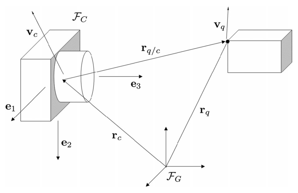
Figure 1: Schematic of the Model [10].

Taking $x=[x_{1},x_{2},x_{3}]^{T}=[\frac{X}{Z},\frac{Y}{Z},\frac{1}{Z}]^{T}\in\Re^{3}$ as the state vector, the continuous-time state space model is obtained as follows

$$\dot{x}_{1}=\Omega_{1}+\zeta_{1}+v_{q1}x_{3}-x_{1}v_{q3}x_{3}$$

$$\dot{x}_{2}=\Omega_{2}+\zeta_{2}+v_{q2}x_{3}-x_{2}v_{q3}x_{3}$$

$$\dot{x}_{3}=v_{c3}x_{3}^{2}-(\omega_{2}x_{1}-\omega_{1}x_{2})x_{3}-v_{q3}x_{3}^{2}$$ (61)

where it is assumed that $v_{q}\triangleq[v_{q1},v_{q2},v_{q3}]$, $v_{c}\triangleq[v_{c1},v_{c2},v_{c3}]$, $\omega\triangleq[\omega_{1},\omega_{2},\omega_{3}]$; besides, $\Omega_{1},\Omega_{2},\zeta_{1},\zeta_{2}:[0,\infty)\times\Re^{3}\rightarrow\Re$ are defined as follows

$$\Omega_{1}(t,x)=\omega_{3}x_{2}-\omega_{2}-\omega_{2}x_{1}^{2}+\omega_{1}x_{1}x_{2}$$

$$\Omega_{2}(t,x)=-\omega_{3}x_{1}+\omega_{1}-\omega_{2}x_{1}x_{2}+\omega_{1}x_{2}^{2}$$

$$\zeta_{1}(t,x)=(v_{c3}x_{1}-v_{c1})x_{3}$$

$$\zeta_{2}(t,x)=(v_{c3}x_{2}-v_{c2})x_{3}$$ (62)

To get comprehensive details about the presented model, refer to [10]. Since the images taken from camera are utilized as observations, the output model is simply $y=[x_{1},x_{2}]^{T}$ as well.

The following assumptions have to be made, in order to employ this model for the proposed filter:
1- Camera velocities $v_{c}$ and $\omega$ are measurable.
2- The first two state variables are bounded and observed continuously by the camera.
3- Object velocities are taken as unknown inputs to the system.
Remark 11: Utilizing projective geometry, the feature point coordinates of the image, $u,v$ are related to the normalized Euclidean one by the following equation:

$$[u\quad v\quad 1]^{T}=A_{c}[Y/Z\quad X/Z\quad 1]^{T}$$ (63)

where $A_{c}\in\Re^{3\times 3}$ is the invertible camera intrinsic parameter matrix [10]. Utilizing (63), the states $x_{1}$ and $x_{2}$ are measurable if assumption 2 holds. This model has a major limitation in 2D motion plane of an autonomous vehicle; having just one state variable, $x_{2}$ observed by the camera, estimating the depth ($x_{3}$) is not possible due to the resulted unobservable model. To solve this problem, a new output model is defined through employing the intercept theorem.

4.2 The Developed Model

In an autonomous vehicle motion plane, there are two degrees of freedom. Since the presented kinematic model is generally in 3D dimension, it has to be reduced to a 2D one which does not consider $x_{1}$. In this regard, $x_{1}$ can be set as a constant known value in (4.1). To have an observable state space, an output model is developed through applying the following theorem.

Theorem 3.

(Thales’ intercept theorem [47]). Consider an arbitrary triangle $ABC$ as in Fig. 2 and let $AC$ be extended to $C^{\prime}$ and $AB$ to $B^{\prime}$, so that $B^{\prime}C^{\prime}$ is parallel to $BC$. Then the lengths of the sides satisfy the relations

$$\frac{a^{\prime}}{a}=\frac{b^{\prime}}{b}=\frac{c^{\prime}}{c}$$ (64)

and hence

$$\frac{a^{\prime}}{c^{\prime}}=\frac{a}{c},\quad\frac{c^{\prime}}{b^{\prime}}=\frac{c}{b},\quad\frac{b^{\prime}}{a^{\prime}}=\frac{b}{a}$$ (65)

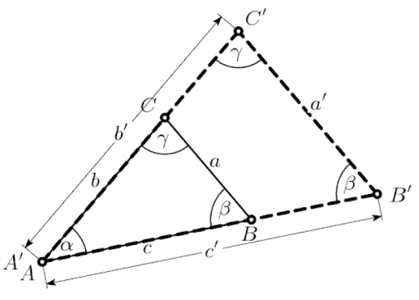
Figure 2: Thales’ intercept theorem [47].

Now consider Fig. 3 to carry on the output model expansion. The main purpose is to estimate $Z$, which is the distance from the object contact point with the ground to the camera pinhole $P$. In this regard, $Y$ is taken as an observation on the image plane and the following relation is obtained through employing theorem 3:

$$\frac{F}{F+Z}=\frac{\tilde{Y}}{\tilde{Y}+H}$$ (66)

where $F$ is the focal length of the camera, $H$ is the height of the camera with respect to the ground, and $Y_{1}=Y-VP$. Note that, $Y_{1}$ is not the observation since it is calculated with respect to the camera center point. Thus, $VP$ is used to modify $Y$. Furthermore, since $Y_{1}$ is in pixel unit, $\tilde{Y}=Y_{1}\frac{h_{f}}{h}$ is utilized as the vertical position of the object in the image plane in which $h$ and $h_{f}$ are the maximum amount of pixels along the height of the camera film and its real height, respectively. Thus, having $F$, $H$ and $Y_{1}$, the depth($Z$) is estimated. However, to utilize this equation as the output model, rewrite (66) as follows

$$F\left(\frac{H}{Z}\right)=\tilde{Y}$$ (67)

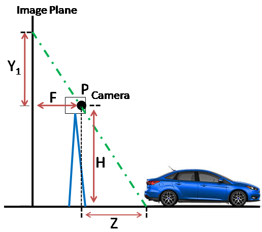
Figure 3: Concept of the developed output model

Remark 12: $h$ and $h_{f}$ are directly related to the sensor dimensions, and they are reported in the camera information. Besides, $VP$ is the vanishing point of the camera.

Since the state vector is defined as $x=(\frac{X}{Z},\frac{Y}{Z},\frac{1}{Z})$, it can be seen that $Z=\frac{1}{x_{3}}$. To obtain $\tilde{Y}$ in terms of the state variables, consider matrix $A_{c}$ in (63) as

$$A_{c}=\left[\begin{matrix}f_{x}&0&x_{0}\\ 0&f_{y}&y_{0}\\ 0&0&1\end{matrix}\right]$$ (68)

where $f_{x}$ and $f_{y}$ are equal to each other and representing the focal length of the camera. Moreover, $x_{0}$ and $y_{0}$ are determined from the distance between the image origin and its center. Then taking into account (68) along (63), $\tilde{Y}$ is obtained as follows:

$$\tilde{Y}=(f_{y}(x_{1})+y_{0})\frac{h_{f}}{h}$$ (69)

Consequently, the output model would be

$$x_{1}=((FHx_{3})\frac{h}{h_{f}}-y_{0})\frac{1}{f_{y}}$$ (70)

There is an important point to note; although $x_{1}$ is taken as a constant value in the state space, the output model can be defined as follows without loss of generality:

$$y=[x_{2},((FHx_{3})\frac{h}{h_{f}}-y_{0})\frac{1}{f_{y}}]^{T}$$ (71)

Note that $x_{1}$ is not considered in (71) due to the assumption made to take this state as a constant known parameter. This output model yields an observable state space which can be employed in the real implementation.

5 Simulation Results

This section is organized as follows: First, simulation results on state estimation based on the general state space form in (4.1) alongside $y=[x_{1},x_{2}]^{T}$ as observation model are analyzed in absence of model uncertainties. Then, the uncertainty in the model is added and its effects are studied. Finally, a Monte Carlo simulation is performed to analyze the robustness of the proposed approach with respect to the other approaches. All simulations are reported based on a comparison study of the proposed filter with an unknown input observer and the common SDRE filter. A point to ponder is that the UIO is a common approach in solving the SFM problem in the literature [10, 11]. Furthermore, this method is designed for estimations in the presence of unknown inputs [10]. Since in this paper the problem is discussed in the presence of unknown inputs in addition to model uncertainties, it is proposed to utilize the proposed switched SDRE method instead. Note that, simulation details are in accordance with [10].

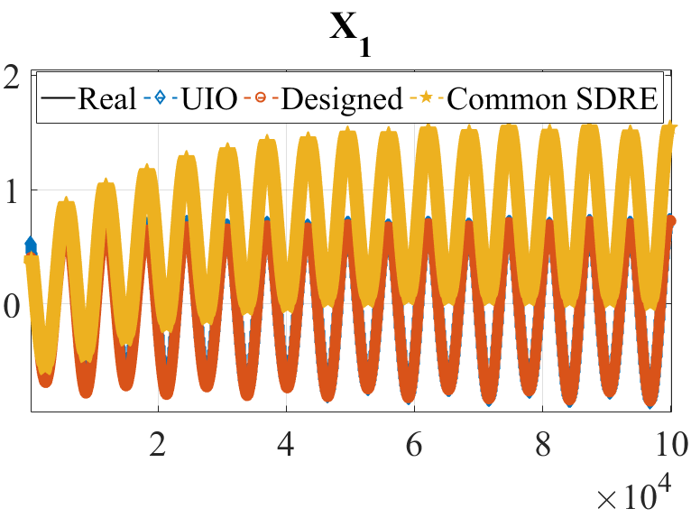
(a)

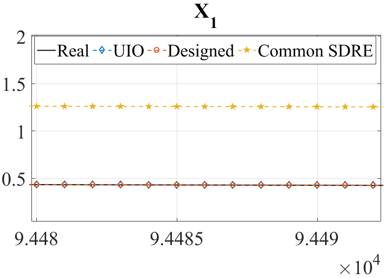
(b) Magnified

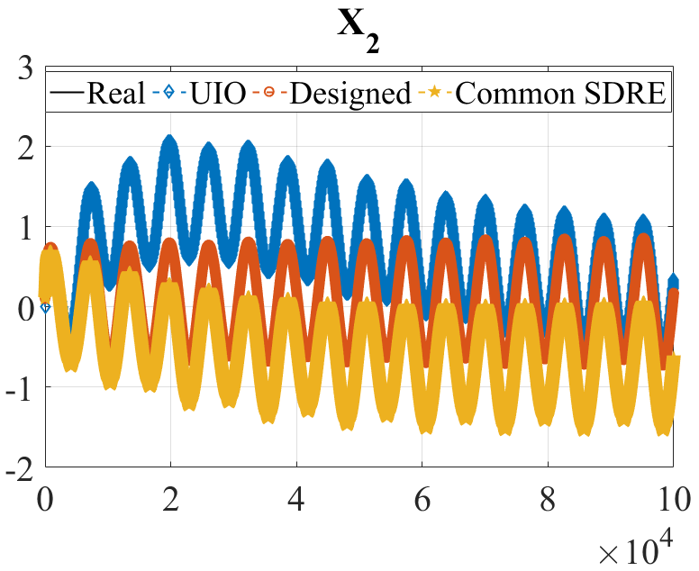
(c)

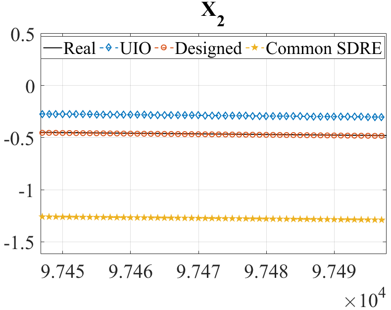
(d) Magnified

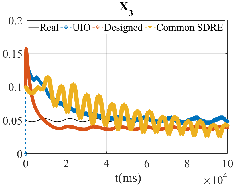
(e)

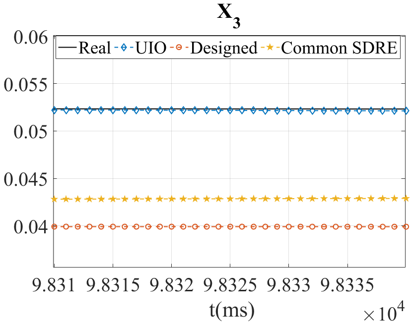
(f) Magnified

Figure 4: Estimation results in absence of uncertainties of the model

Remark 13: To discretize the continuous-time model in (4.1), Euler method [48] is employed to preserve stability in the conversion.

Fig. 4 displays the results of the three mentioned methods for estimation of an object Euclidean position where the uncertainties are not present. As it can be seen in the simulation results, especially looking into the magnified plots, the UIO performance is better compared to the other approaches due to the complete elimination of disturbance effects. This is reported to ensure the efficiency of the UIO method in an ideal condition. Furthermore, improvement in the common SDRE filter operation by utilizing the switching concept in the designed approach is also clear specially in $x_{1}$ and $x_{2}$ states. Note that although there is no uncertainty in the model, the external disturbance results in an error in estimations which can be minimized through switching of covariance matrix in the proposed filter. Next, to take into account the model uncertainties, process and measurement noises along with uncertainties in the camera, uncertainty in linear velocity is considered, in which it is assumed that the linear velocity of the camera, $V_{c}$ is $80\%$ of its real value. In other words, it is assumed that the $V_{c}$ exact value is not accessible and an approximation is taken. Furthermore, noises are considered to keep in view the existing vibration in the device in which the camera is mounted on. Likewise, the design parameters of the approaches are set to be the same as the previous simulation. As it is delineated in Fig. 5, the performance of the proposed filter is much better than the others. Both variance and mean value of estimation error are lower for the designed filter and it is clear that the proposed method has gained robust performance due to its switching essence.

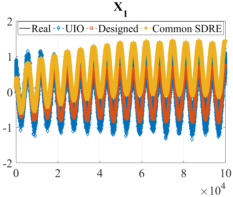
(a)

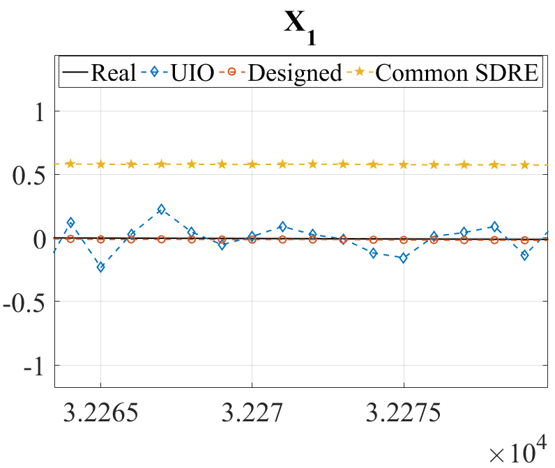
(b) Magnified

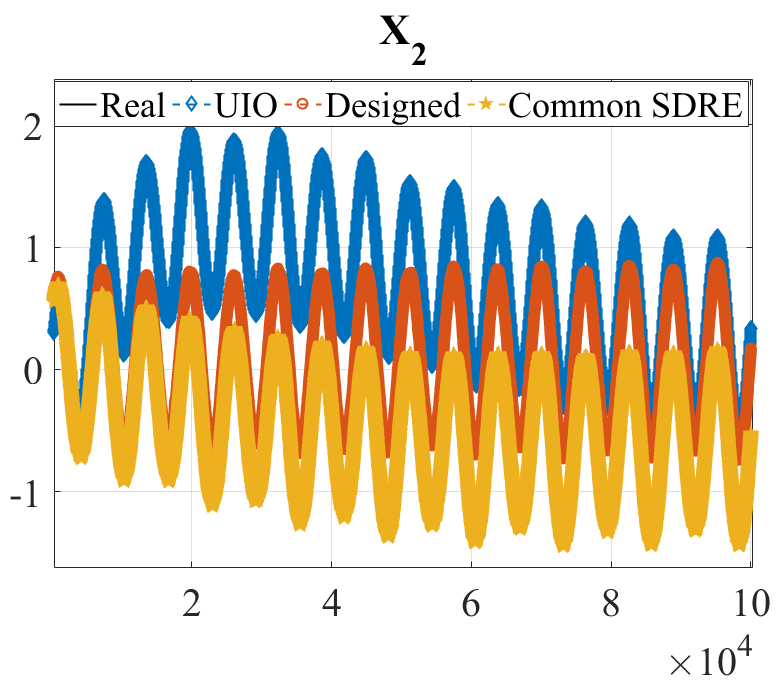
(c)

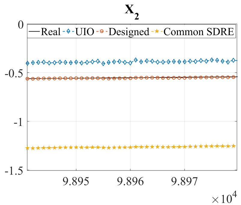
(d) Magnified

(e)

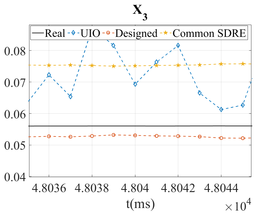
(f) Magnified

Figure 5: Estimation results in presence of uncertainties of the model, utilizing the same design parameters as in Fig. 4

To further investigate the robustness of the suggested approach, a Monte-Carlo simulation is performed in which the camera linear velocity is assumed to be partially known as an stochastic process in a range from $50\%$ to $150\%$ of its real value. To clarify, the simulation is accomplished on $1000$ different amounts of $V_{c}$ in the interval of $[0.5V_{c},1.5V_{c}]$ and for each simulation, the estimations are obtained through utilizing the three mentioned methods for about 10$sec$ with 1$ms$ sampling-rate.

Remark 14: To take $V_{c}$ as uncertainty, each of its elements is considered as a stochastic value independently.

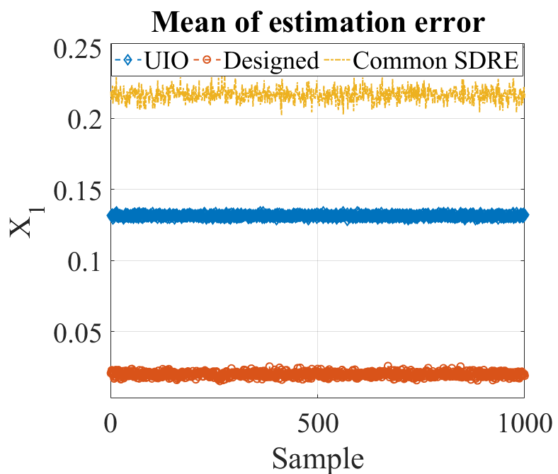
(a)

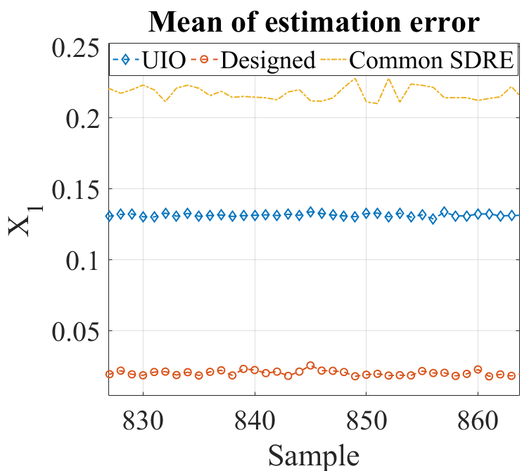
(b) Magnified

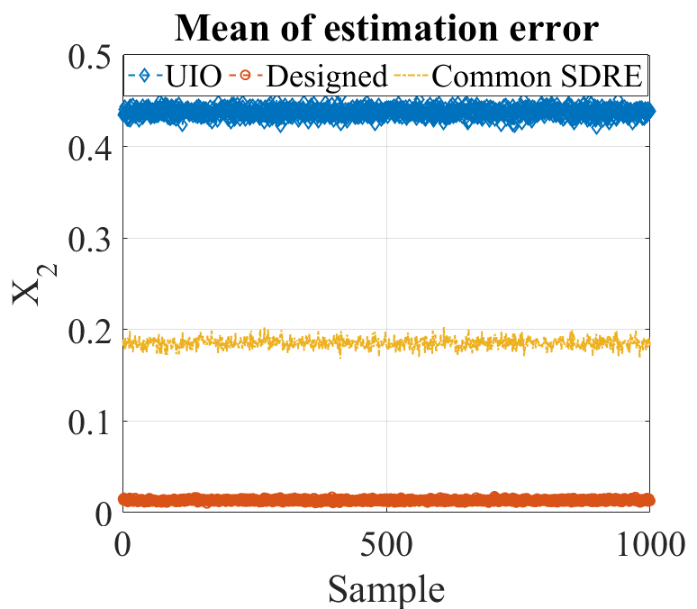
(c)

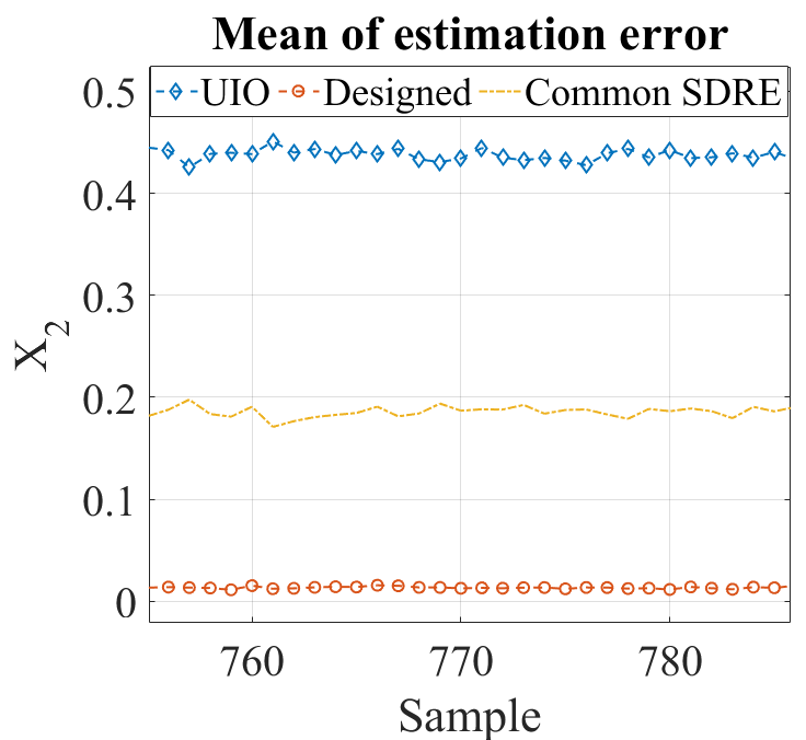
(d) Magnified

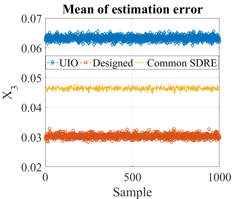
(e)

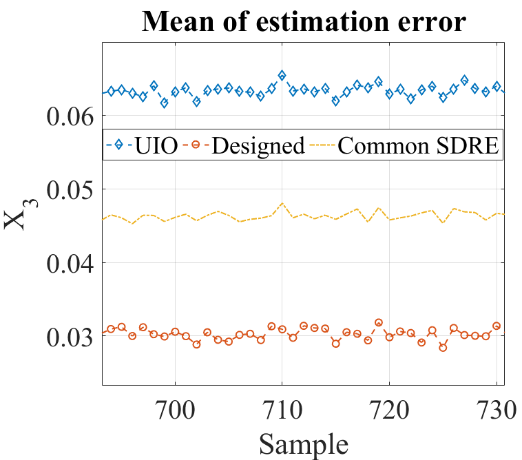
(f) Magnified

Figure 6: Mean value of estimation error as a result of Monte-Carlo simulation

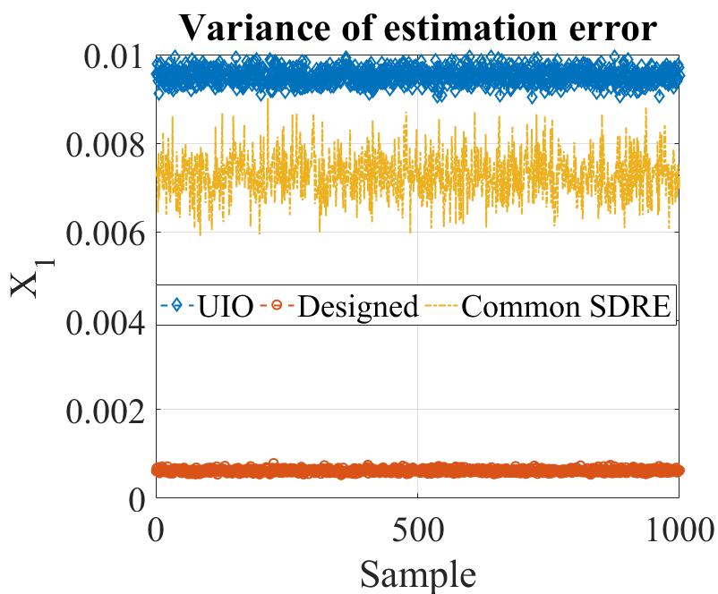
(a)

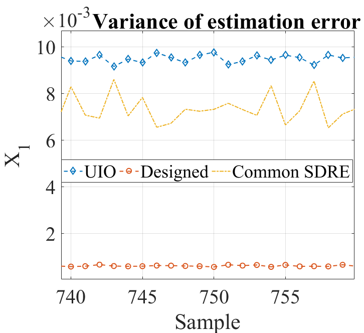
(b) Magnified

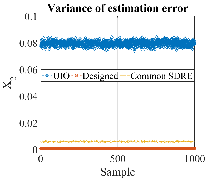
(c)

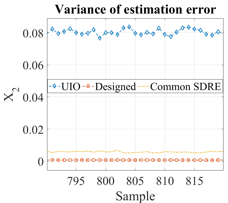
(d) Magnified

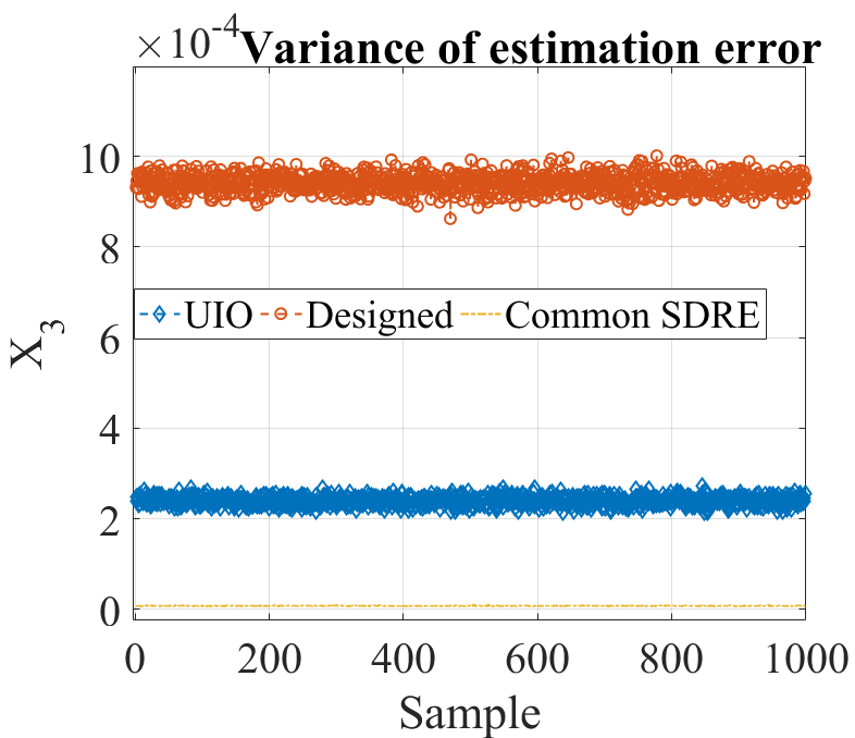
(e)

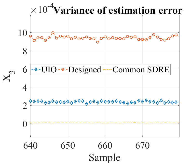
(f) Magnified

Figure 7: Variance of the estimation error as a result of Monte-Carlo simulation

As a result of the Monte-Carlo simulation, the estimation error mean value is shown in Fig. 6. This index is much lower for the designed filter in estimating all the three state variables. The other important touchstone is the variance of estimation error which is given in Fig .7. It is seen that the estimation error variance of the proposed method is much lower than the others in other two methods in $x_{1}$ and $x_{2}$ estimation. However, this is not the case for the third state $x_{3}$, but the amount of this variance is of order $10^{-4}$ and less important than the other two states estimation. Consequently, utilizing switching improves the robustness of the common SDRE and yields a robust performance in the presence of model uncertainties compared even to UIO filter.

6 Experimental Results

In this section, experimental results are presented in which both longitudinal and lateral distances of frontal dynamic objects are estimated for a host vehicle. The overall experimental setup is illustrated in Fig. 8. The camera is located as indicated on the right, while the Jetson Tx2 is seen on the left.

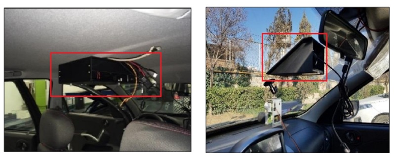
Figure 8: The experimental setup

In what follows, first, the concept of employing CNNs alongside an OpenCV tracker is presented. Later the mentioned model in (4.1) is reduced to a fourth-order state space due to having a 2D motion plane. Then the output model developed in (71) is analyzed for possible employment as an observable system. Finally, to verify the proposed algorithm, the radar data is utilized and the estimation values are compared to that of the radar measurements. To get a proper intuition on the proposed approach, the block diagram of the whole system implemented in the experiments is presented in Fig. 9. As it is seen in this figure, camera images are processed by a robust tracker that contains both YOLO CNN and the median flow OpenCV tracker. The outputs of this block are the observations that are used in the proposed estimator to estimate both longitudinal and lateral distances. In the literature, almost all researches reported using a pre-mounted sign on the object in performing experiments, although it is a serious limitation for these approaches when it comes to the real applications. To tackle this problem, in this paper a CNN is utilized to detect all potential moving objects through a single image. In addition, considering the reported results in [49], employing CNNs beside a Median-flow tracker yields a promising performance in tracking objects through image sequences. Consequently, after the initial detection and feeding of the tracker, every ’$n$’ frames the YOLO CNN is re-executed to detect new objects and modify the tracker, to result in a real-time and robust performance implementation. Furthermore, coordinates of the object contact point with the ground are utilized as observations and inputs to the proposed filter to estimate lateral and longitudinal distances. The reduced state space model to be used for the proposed filter is presented as:

$$x(k+1)=A(x(k))x(k)+B_{1}(x(k))V_{c}(k)+B_{2}(x(k))\omega(k)$$ (72)

in which $\omega$ and $V_{c}$ are the angular and linear velocities of the camera, respectively, and

$$A(x(k))=\left[\begin{matrix}1&-\frac{T}{2}(x_{2}x_{6})_{k}&\frac{T}{2}(x_{3})_{k}&0\\ 0&1&0&-\frac{T}{2}(x_{3}^{2})_{k}\\ 0&0&1&0\\ 0&0&0&1\end{matrix}\right]$$ (73)

$$B_{1}(x(k))=\left[\begin{matrix}0&-\frac{T}{2}(x_{3})_{k}&\frac{T}{2}(x_{2}x_{3})_{k}\\ 0&0&\frac{T}{2}(x_{3}^{2})_{k}\\ 0&0&0\\ 0&0&0\end{matrix}\right]$$ (74)

$$B_{2}(x(k))=\left[\begin{matrix}\frac{T}{2}(1+x_{2}^{2})_{k}&-\frac{T}{2}(x_{1}x_{2})_{k}&-\frac{T}{2}(x_{1})_{k}\\ \frac{T}{2}(x_{2}x_{3})_{k}&-\frac{T}{2}(x_{1}x_{3})_{k}&0\\ 0&0&0\\ 0&0&0\\ \end{matrix}\right]$$ (75)

while the output model is:

$$y(k)=h(x(k))x(k)$$ (76)

It is noteworthy to mention that here $x(k)$ is equal to $[x_{2},x_{3},x_{5},x_{6}]^{T}$ where $x_{5}$ and $x_{6}$ are $V_{q2}$ and $V_{q3}$, respectively. Note that, $x_{1}$ is taken as a constant value in these equations which yields $x_{4}$ to be zero.

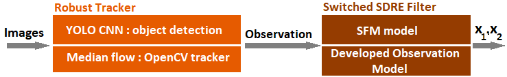
Figure 9: Block diagram of the suggested approach

Remark 15: A vital thing for having a practical approach is to optimize the framework as much as possible to further enhance the performance. Utilizing YOLO at each frame may result in better performance. However, the computational cost is far higher than that of the proposed algorithm of using YOLO alongside medianflow tracker.

Since the camera has some parameters which are used in (71), it is imperative to calibrate this observation model before the implementation. In this regard, a data set is used which consists of both radar and image data. This data set is gathered through a scenario in which a car has a sweeping movement. Applying YOLOv3 on the images results in the bounding boxes for each image, and this may be utilized to attain a function which relates the contact points of the objects with the ground, to the frontal distances.

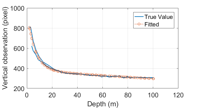
(a)

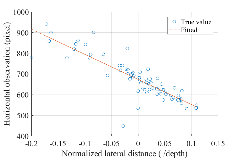
(b)

Figure 10: Nonlinear functions derived from plotting vertical and horizontal observations with respect to the true depth and the normalized lateral distance taken from the radar data

Fig. 10a indicates the nonlinear behavior of the practical vertical observations with respect to the ground truth longitudinal distances. As it is seen in this figure, due to the inherent nonlinear behavior of these states, a linear model would not be sufficient to be used as the observation model. Consequently, an alternative is to use multiple linear models considering (71), or to use a persistent nonlinear model to encapsulate this behavior. In this paper we propose using such model for the whole range of distances up to $100$ meters. To this end, the following nonlinear function is fitted on the ground truth data as shown in Fig. 10a.

$$y_{2}=588\exp{(-0.161\frac{1}{x_{3}})}+382.6\exp{(-0.002547\frac{1}{x_{3}})}$$ (77)

Using the same approach, Fig. 10b depicts the relation between normalized lateral distance and horizontal observations. Since there is no need to use a nonlinear function in here, the normalized lateral distance is employed in a linear function to fit the empirical observations as follows:

$$y_{1}=-1214x_{2}+673.6$$ (78)

Use (77), (78) into (76), to finalize the observation model as:

$$h(x(k))=\left[\begin{matrix}\frac{y_{1}}{x_{2}}&0&0&0\\ 0&\frac{y_{2}}{x_{3}}&0&0\end{matrix}\right].$$ (79)

Note that, since $x_{2}$ goes to zero when both the object and the host car are in a same line, it is essential to omit the constant term in (78), and to consider it as another input to the system.

To achieve real-time performance on an Nvidia Jetson Tx2 board, tiny YOLO [19] has been used, which yields a limitation in depth estimation range. Note that by utilizing YOLOv3, depth estimation is valid up to $100$ meters. However, in tiny YOLO this range is limited to about $40$ meters. In fact, the restriction is applied by the CNN structure, while more layers result in the detection of farther objects. Albeit both CNNs are employed in this research, the results of utilizing YOLOv3 are reported to evaluate the whole algorithm for the range of $100$ meters. Moreover, a multi-thread framework is designed to extend this algorithm to multi-object tracking applications in which there is a main thread responsible for producing observations, and for each object a thread is created which will be executed for the estimation of the lateral and longitudinal distances of that object. By this means the proposed method is generalized for any number of the objects in the scene.

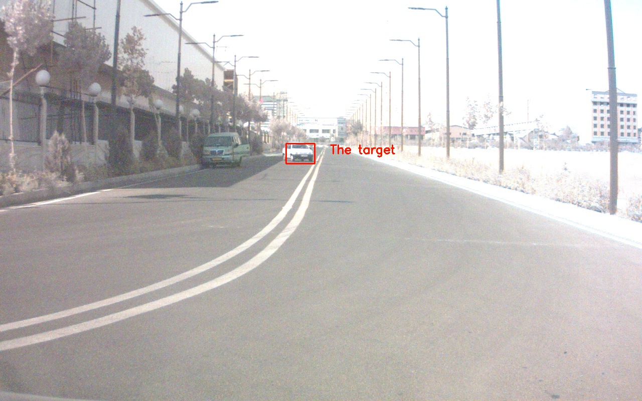
(a)

(b)

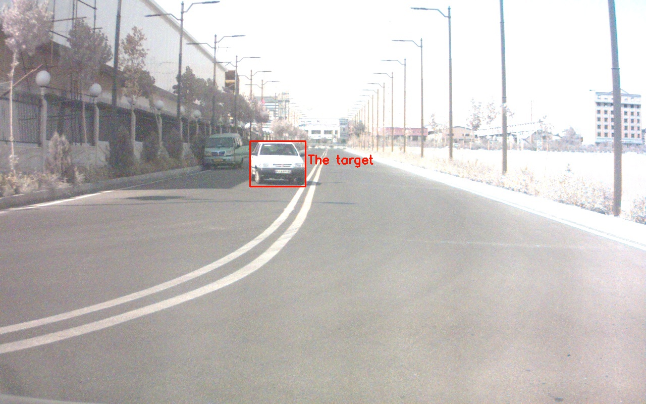
(c)

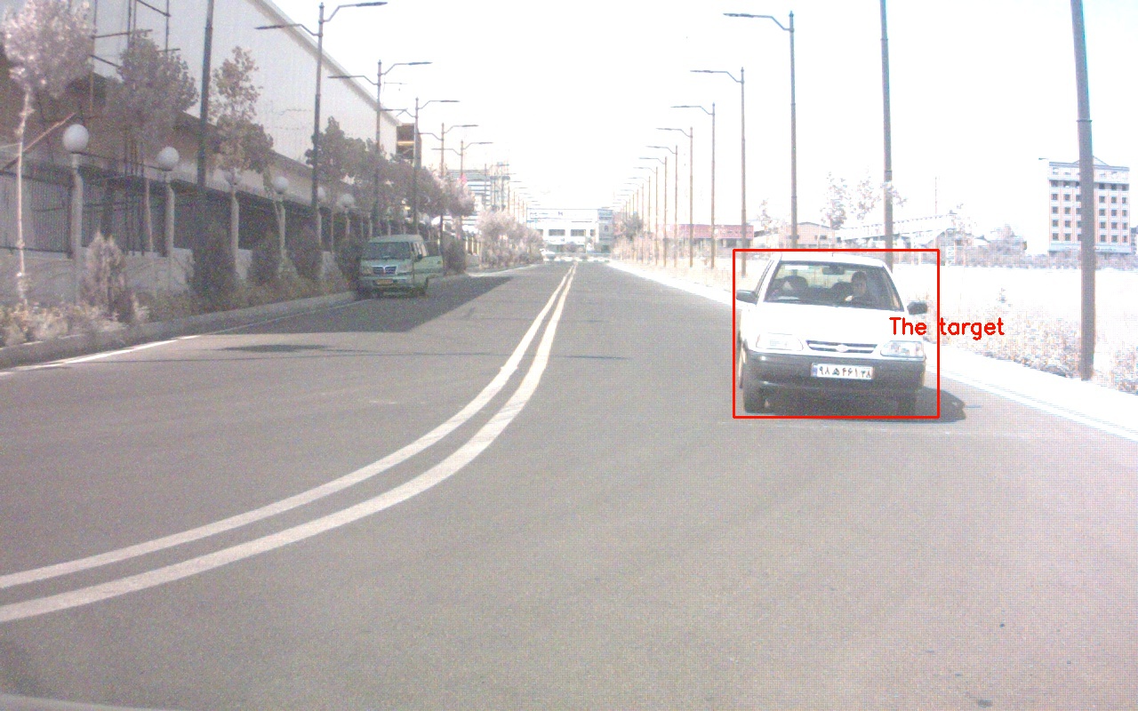
(d)

Figure 11: Sample images of the test scenario

Experiments are conducted on a video sequence utilizing the aforementioned model. The video encompasses $34$ frames which $4$ of them are reported in Fig. 11. The experiment scenario is designed such that a vehicle comes toward the host car with a curly maneuver, with the aim to estimate the lateral and longitudinal distances of the moving car by using a monocular camera. In fact, the scenario represents an exaggerated motion of the frontal car as a critical situation in which the driver has lost the vehicle control, and it comes to the left lane and in front of the host car.

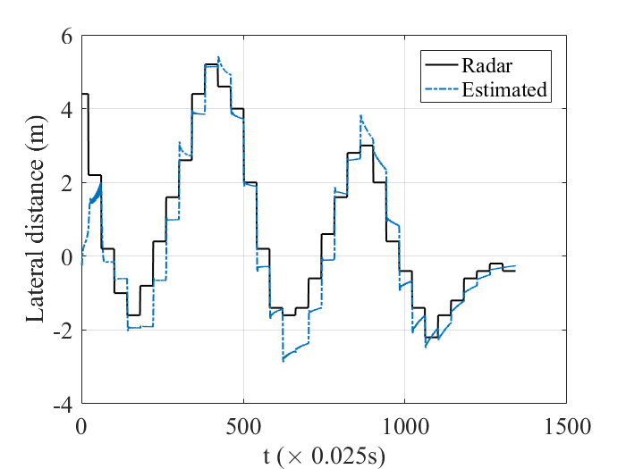
(a)

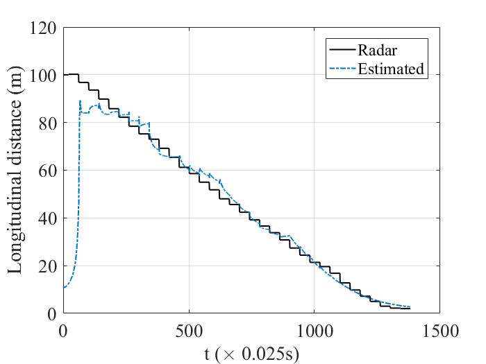
(b)

Figure 12: Estimated longitudinal and lateral distances

Fig. 12 depicts the proposed results in lateral and longitudinal distance estimation, while as mentioned earlier, radar data has been used to verify the accuracy of the results. As it can be seen, the proposed algorithm suitably determines the movement pattern of the object precisely, and furthermore, it estimates the absolute value of the lateral distance efficiently. In fact, according to this result, the estimation error for the longitudinal distance is impressively less than $3\%$ for the range below $50$ meters, and this increases to just $5\%$ for the range of $70$ meters. Compared to the results of the presented machine learning based approaches in the literature [34], the accuracy is at least two times higher while the estimation is performed in a dynamic scene. In fact, this is the first approach presented in the literature which covers the estimation problem of both longitudinal and lateral distances in a tracking scenario, and more importantly, for a practical application. Note that, the camera is not expected to yield very accurate results for farther objects, while this causes no problem in applications such as obstacle avoidance, since the suggested method performs well in the required operation range. Another important point to ponder is, regarding the estimation equations, any error in the longitudinal distance estimation directly effects on the lateral distance one which further demonstrate the applicability of the proposed approach since the results for the lateral distance are promising with almost no drift.

Remark 16: The main thread which produces the observations, is much slower compared to the other threads. Thus, results in Fig. 12 are prone to be in a zero-order hold (ZOH) form.

Remark 17: The framework has been implemented such that for each object in the image, a distinct thread is set. Each of these threads consists of an SFM module with about $1ms$ computation time. As a result, the proposed algorithm performs in real-time, and it is applicable in real-world applications.

7 Conclusions

In this article, a framework is suggested to detect and track frontal dynamic objects in an autonomous vehicle motion plane. First, a switched SDRE filter is proposed as an effective method to solve the general form of the SFM problem in the presence of uncertainties, compared to that of commonly used UIO method. To analyze the robustness of the proposed approach, a Monte Carlo simulation is performed and a comparative study on three filters reveals the effectiveness of the proposed method. By utilizing a newly developed observation model alongside the SFM, an observable model for an autonomous vehicle in motion plane is derived. Moreover, to obtain observations from a monocular camera, CNNs are employed beside the Median-flow tracker. Reported simulation results verify the theoretical development of the proposed filter. As a result, the Monte Carlo simulation indicates the superiority of the proposed switched SDRE filter among both the commonly used UIO approach and the common SDRE. Considering both the mean and the variance of the estimation error, the suggested estimator has lower indexes in the presence of uncertainties. In order to have a real-time implementation in practice, a multi-thread framework is implemented. Experimental results show a promising performance in frontal distance estimation. Our future research is focused on the expansion of the experiments to the cases with intermittent observations, in which recurrent neural networks may assist for better estimation of the frontal object positions.

References

References

- [1] Y. Cao, Z. Wu, C. Shen, Estimating depth from monocular images as classification using deep fully convolutional residual networks, IEEE Transactions on Circuits and Systems for Video Technology 28 (11) (2018) 3174–3182.
- [2] F. Liu, C. Shen, G. Lin, I. D. Reid, Learning depth from single monocular images using deep convolutional neural fields., IEEE Trans. Pattern Anal. Mach. Intell. 38 (10) (2016) 2024–2039.
- [3] C. Godard, O. Mac Aodha, G. J. Brostow, Unsupervised monocular depth estimation with left-right consistency, in: CVPR, Vol. 2, 2017, p. 7.
- [4] T. Zhou, M. Brown, N. Snavely, D. G. Lowe, Unsupervised learning of depth and ego-motion from video, in: CVPR, Vol. 2, 2017, p. 7.
- [5] C. Zhao, Q. Sun, C. Zhang, Y. Tang, F. Qian, Monocular depth estimation based on deep learning: An overview, Science China Technological Sciences (2020) 1–16.
- [6] J. L. Schonberger, J.-M. Frahm, Structure-from-motion revisited, in: Proceedings of the IEEE Conference on Computer Vision and Pattern Recognition, 2016, pp. 4104–4113.
- [7] M. Smith, J. Carrivick, D. Quincey, Structure from motion photogrammetry in physical geography, Progress in Physical Geography 40 (2) (2016) 247–275.
- [8] X. Wei, Y. Zhang, Z. Li, Y. Fu, X. Xue, Deepsfm: Structure from motion via deep bundle adjustment, in: European conference on computer vision, Springer, 2020, pp. 230–247.
- [9] M. Humenberger, Y. Cabon, N. Guerin, J. Morat, J. Revaud, P. Rerole, N. Pion, C. de Souza, V. Leroy, G. Csurka, Robust image retrieval-based visual localization using kapture, arXiv preprint arXiv:2007.13867.
- [10] D. Chwa, A. P. Dani, W. E. Dixon, Range and motion estimation of a monocular camera using static and moving objects., IEEE Trans. Contr. Sys. Techn. 24 (4) (2016) 1174–1183.
- [11] A. Parikh, T.-H. Cheng, H.-Y. Chen, W. E. Dixon, A switched systems framework for guaranteed convergence of image-based observers with intermittent measurements, IEEE Transactions on Robotics 33 (2) (2017) 266–280.
- [12] G. Hu, D. Aiken, S. Gupta, W. E. Dixon, Lyapunov-based range identification for paracatadioptric systems, IEEE Transactions on Automatic Control 53 (7) (2008) 1775–1781.
- [13] P. Yang, W. Wu, Efficient particle filter localization algorithm in dense passive rfid tag environment, IEEE Transactions on Industrial Electronics 61 (10) (2014) 5641–5651.
- [14] S. Sayeef, G. Foo, M. F. Rahman, Rotor position and speed estimation of a variable structure direct-torque-controlled ipm synchronous motor drive at very low speeds including standstill, IEEE Transactions on Industrial Electronics 57 (11) (2010) 3715–3723.
- [15] H. Kim, J. Son, J. Lee, et al., A high-speed sliding-mode observer for the sensorless speed control of a pmsm, IEEE Transactions on Industrial Electronics 58 (9) (2011) 4069–4077.
- [16] N. Davidson, A. Wixner, M. Majji, A. S. Blake, C. I. Restrepo, Extended kalman filtering for vision based terrain relative navigation, in: AIAA Scitech 2019 Forum, 2019, p. 1179.
- [17] T. Cimen, Survey of state-dependent riccati equation in nonlinear optimal feedback control synthesis, Journal of Guidance, Control, and Dynamics 35 (4) (2012) 1025–1047.
- [18] K. Zhang, N. Liu, X. Yuan, X. Guo, C. Gao, Z. Zhao, Z. Ma, Fine-grained age estimation in the wild with attention lstm networks, IEEE Transactions on Circuits and Systems for Video Technology.
- [19] J. Redmon, A. Farhadi, Yolov3: An incremental improvement, arXiv preprint arXiv:1804.02767.
- [20] K. Zhang, M. Sun, T. X. Han, X. Yuan, L. Guo, T. Liu, Residual networks of residual networks: Multilevel residual networks, IEEE Transactions on Circuits and Systems for Video Technology 28 (6) (2017) 1303–1314.
- [21] J. Huang, V. Rathod, C. Sun, M. Zhu, A. Korattikara, A. Fathi, I. Fischer, Z. Wojna, Y. Song, S. Guadarrama, et al., Speed/accuracy trade-offs for modern convolutional object detectors, in: IEEE CVPR, Vol. 4, 2017.
- [22] G. Bradski, The OpenCV Library, Dr. Dobb’s Journal of Software Tools.
- [23] Z. Kalal, K. Mikolajczyk, J. Matas, et al., Tracking-learning-detection, IEEE transactions on pattern analysis and machine intelligence 34 (7) (2012) 1409.
- [24] Z. Kalal, K. Mikolajczyk, J. Matas, Forward-backward error: Automatic detection of tracking failures, in: Pattern recognition (ICPR), 2010 20th international conference on, IEEE, 2010, pp. 2756–2759.
- [25] S. Nazari, The unknown input observer and its advantages with examples, arXiv preprint arXiv:1504.07300.
- [26] Y. Guan, M. Saif, A novel approach to the design of unknown input observers, IEEE Transactions on Automatic Control 36 (5) (1991) 632–635.
- [27] B. Marx, D. Ichalal, J. Ragot, D. Maquin, S. Mammar, Unknown input observer for lpv systems, Automatica 100 (2019) 67–74.
- [28] S. Jang, A. P. Dani, C. D. Crane III, W. E. Dixon, Experimental results for moving object structure estimation using an unknown input observer approach, in: Dynamic Systems and Control Conference, Vol. 45301, American Society of Mechanical Engineers, 2012, pp. 597–606.
- [29] A. P. Dani, Z. Kan, N. R. Fischer, W. E. Dixon, Structure estimation of a moving object using a moving camera: An unknown input observer approach, in: 2011 50th IEEE Conference on Decision and Control and European Control Conference, IEEE, 2011, pp. 5005–5010.
- [30] H. H. Alhelou, Fault detection and isolation in power systems using unknown input observer, Advanced condition monitoring and fault diagnosis of electric machines (2019) 38–58.
- [31] J. Zhu, Y. Fang, Learning object-specific distance from a monocular image, in: Proceedings of the IEEE/CVF International Conference on Computer Vision, 2019, pp. 3839–3848.
- [32] Y. Zhang, Y. Li, M. Zhao, X. Yu, A regional regression network for monocular object distance estimation, in: 2020 IEEE International Conference on Multimedia & Expo Workshops (ICMEW), IEEE, 2020, pp. 1–6.
- [33] R. Girshick, J. Donahue, T. Darrell, J. Malik, Rich feature hierarchies for accurate object detection and semantic segmentation, in: Proceedings of the IEEE conference on computer vision and pattern recognition, 2014, pp. 580–587.
- [34] M. A. Haseeb, J. Guan, D. Ristic-Durrant, A. Gräser, Disnet: a novel method for distance estimation from monocular camera, 10th Planning, Perception and Navigation for Intelligent Vehicles (PPNIV18), IROS.
- [35] J. Redmon, Darknet: Open source neural networks in c, http://pjreddie.com/darknet/ (2013–2016).
- [36] T.-s. Lou, X.-q. Wang, H.-m. Zhao, Z.-w. Chen, Robust partly strong tracking consider sdre filter for direct ins/gnss integration with biases, Measurement Science and Technology 31 (11) (2020) 115016.
- [37] H. Rouzegar, A. Khosravi, P. Sarhadi, Spacecraft formation flying control around l2 sun-earth libration point using on–off sdre approach, Advances in Space Research.
- [38] M. Wang, X. Dong, X. Ren, Q. Chen, Sdre based optimal finite-time tracking control of a multi-motor driving system, International Journal of Control (2020) 1–13.
- [39] A. Bavarsad, A. Fakharian, M. B. Menhaj, Nonlinear observer-based optimal control of an active transfemoral prosthesis, Journal of Central South University 28 (1) (2021) 140–152.
- [40] F. Lotfi, S. Ziapour, F. Faraji, H. D. Taghirad, A switched sdre filter for state of charge estimation of lithium-ion batteries, International Journal of Electrical Power and Energy Systems , https://authors.elsevier.com/c/1a84zWJH6PHhE.
- [41] T. Cimen, Systematic and effective design of nonlinear feedback controllers via the state-dependent riccati equation (sdre) method, Annual Reviews in Control 34 (1) (2010) 32–51.
- [42] D. Simon, Optimal state estimation: Kalman, H infinity, and nonlinear approaches, John Wiley & Sons, 2006.
- [43] J. Baras, A. Bensoussan, M. James, Dynamic observers as asymptotic limits of recursive filters: Special cases, SIAM Journal on Applied Mathematics 48 (5) (1988) 1147–1158.
- [44] H. Banks, B. Lewis, H. Tran, Nonlinear feedback controllers and compensators: a state-dependent riccati equation approach, Computational Optimization and Applications 37 (2) (2007) 177–218.
- [45] L. Zhang, Y. Zhu, P. Shi, Q. Lu, Time-dependent switched discrete-time linear systems: Control and filtering, Springer, 2016.
- [46] Z. Ding, G. Cheng, A new uniformly ultimate boundedness criterion for discrete-time nonlinear systems, Applied Mathematics 2 (11) (2011) 1323.
- [47] A. Ostermann, G. Wanner, Geometry by its history, Springer Science & Business Media, 2012.
- [48] J. C. Butcher, Numerical methods for ordinary differential equations, John Wiley & Sons, 2016.
- [49] F. Lotfi, V. Ajallooeian, H. Taghirad, Robust object tracking based on recurrent neural networks, in: 2018 6th RSI International Conference on Robotics and Mechatronics (IcRoM), IEEE, 2018, pp. 507–511.