A High-Gain Observer Approach to Robust Trajectory Estimation and Tracking for a Multi-rotor UAV

Abstract

We study the problem of estimating and tracking an unknown trajectory with a multi-rotor UAV in the presence of modeling error and external disturbances. The reference trajectory is unknown and generated from a reference system with unknown or partially known dynamics. We assume the only measurements that are available are the position and orientation of the multi-rotor and the position of the reference system. We adopt an extended high-gain observer (EHGO) estimation framework to estimate the unmeasured multi-rotor states, modeling error, external disturbances, and the reference trajectory. We design a robust output feedback controller for trajectory tracking that comprises a feedback linearizing controller and the EHGO. The proposed control method is rigorously analyzed to establish its stability properties. Finally, we illustrate our theoretical results through numerical simulation and experimental validation in which a multi-rotor tracks a moving ground vehicle with unknown trajectory and dynamics and successfully lands on the vehicle while in motion.

I Introduction

Multi-rotor UAVs are being deployed in an ever increasing variety of scenarios, from surveillance and remote infrastructure monitoring, to search and rescue and parcel delivery. With the broadening of use cases, performance improvements must be made through hardware, software, and control design to increase flight performance and robustness to unpredictable flight conditions. Much work has been devoted to studying multi-rotor UAV control design; see [2, 3] for a survey. Specifically, efforts have been focused on control advancements to enable aggressive maneuvers [4, 5, 6], react to external disturbances and potential modeling error [7, 8, 9, 10], and to design feasible flight trajectories [11, 12, 13].

Numerous linear and nonlinear control approaches have been applied to multi-rotors, including PID [6, 14], feedback linearization [9, 15, 16], backstepping [17, 18], adaptive control [8, 7, 19], and model predictive control (MPC) [4, 20] to name a few. Linear methods are effective near the hover configuration, but can experience degraded performance during aggressive maneuvers. Feedback linearization is sensitive to sensor noise as well as model uncertainty [16], but results in a linear system which is simple to analyze. Adaptive control and backstepping are often combined to enable a nonlinear adaptive control design [8, 10]. This enables unknown system parameters to be estimated during operation to reduce the effect of model uncertainty. MPC enables excellent tracking performance and can achieve aggressive maneuvers [4], but at the cost of computational complexity.

Additionally, many linear and nonlinear approaches are subject to reduced performance in the presence of model uncertainty and external disturbances [21]. This motivates the use of robust methods which can overcome certain classes of disturbances utilizing observers [21, 22] or adaptive approaches to estimate model parameters online [10, 19]. The magnitude of disturbance that can be canceled may depend on the control gains, which can be tuned using an adaptive gain scheduling approach [21].

Several methods of trajectory generation have also been developed for multi-rotors. Methods applying motion primitives to generate feasible trajectories [13, 12] have been explored and extended specifically to utilize reinforcement learning [12]. Computationally efficient methods which can be implemented and updated in real-time have been developed to design trajectories that also meet dynamic feasibility constraints [11].

While other methods may only address a subset of these challenges, we provide a unified framework which can ensure flight performance under model uncertainties, external disturbances, and unknown reference trajectory dynamics. We design a robust feedback linearizing control strategy that can achieve excellent transient tracking performance even in the presence of these disturbances. Our framework enables real-time trajectory generation based on position information of a reference system which may have partially known or completely unknown dynamics. Furthermore, the magnitude of disturbance this method can overcome is not dependent on control gains, but rather on observer gains. This allows total freedom in assigning control gains, which can be chosen to shape the transient response as we recover the performance of a desired linear system.

To showcase the performance of our method, we will apply our technique to the problem of landing a multi-rotor on a mobile platform [23, 24]. Multiple control methodologies have been applied to this problem, including model predictive control [25, 26], PI control [27, 28, 29], and feedback linearizing control [30]. Many approaches either do not consider modeling error and external disturbances, or consider them to be constant or slowly time-varying [27, 28]. In contrast, our approach only requires that any uncertainty be bounded and continuously differentiable.

State estimators such as a Kalman filter have been used to estimate the dynamic state of the mobile platform [29, 31] under the assumptions that the dynamic model of the mobile platform is known and it travels with unknown, but constant, velocity. Through our EHGO design, these assumptions are relaxed, requiring no information about the dynamics or input of the mobile platform. An alternative approach to estimate the state of the mobile platform uses optical flow data [27, 28], or visual cue data [32] in which a dynamic model of the mobile platform is not required. In these cases the relative velocity is estimated through the optical flow algorithms and is minimized in the control to ensure tracking. The proposed approach relies on relative position measurements and is complimentary to optical flow methods.

The contributions of this work include the design and rigorous analysis of an EHGO based feedback linearizing control method that incorporates estimation of a reference trajectory from an unknown, or partially known, reference dynamic system. The EHGO enables estimation of all states for output feedback control, as well as estimating modeling error and external disturbances, enabling the design of a robust feedback linearizing control strategy. The proposed method can recover performance of the desired linear system under a broad class of disturbances. Existing multi-rotor control techniques require the rotational dynamics to be sufficiently faster than the translational dynamics such that the tracked rotational trajectory can serve as virtual control for the translational subsystem. The proposed EHGO design treats the transient of the rotational subsystem as a disturbance, estimates it, and actively compensates for it in the rotational controller. Thus, the proposed controller does not require the timescale separation between rotational and translational subsystems. A key challenge in implementing an EHGO based output feedback controller is that the dynamics of commercial electronic speed controllers evolve at the same timescale as the EHGO and should be included in EHGO design. We illustrate the influence of inclusion/non-inclusion of these dynamics on output feedback performance. We illustrate the effectiveness of our output feedback controller through simulation and experimental results using the example of landing a multi-rotor on a moving ground vehicle.

The remainder of the paper is organized as follows. The system dynamics are introduced in Section II with the control and observer design in Section III. The controller is analyzed in Section IV and is validated through simulation in Section V with experimental results presented in Section VI. Conclusions are presented in Section VII. Detailed proofs of the technical results are provided in the appendix.

II System Dynamics

In this section, we review the dynamics of the different subsystems of a multi-rotor UAV and reference system.

II-A Rotational Dynamics

The rotational dynamics of the multi-rotor are

$$\boldsymbol{\tau}=J\dot{\Omega}+\Omega\times J\Omega,$$ (1)

where $J\in\mathbb{R}^{3\times 3}$ is the inertia matrix, $\boldsymbol{\tau}\in\mathbb{R}^{3}$ is the torque applied to the multi-rotor body and $\Omega\in\mathbb{R}^{3}$ is the angular velocity, each expressed in the body-fixed frame [33].

Consider the orientation of the multi-rotor expressed in terms of Z-Y-X Euler angles $\boldsymbol{\vartheta}_{1}=[\phi\ \theta\ \psi]^{\top}\in(-\frac{\pi}{2},\frac{\pi}{2})^{2}\times(-\pi,\pi]$. The angular velocity $\Omega$ is related to the Euler angle rates $\boldsymbol{\vartheta}_{2}=[\dot{\phi}\ \dot{\theta}\ \dot{\psi}]^{\top}\in\mathbb{R}^{3}$ in the inertial frame as

$$\boldsymbol{\vartheta}_{2}=\Psi\Omega,\quad\Psi=\left[\begin{matrix}1&s_{\phi}t_{\theta}&c_{\phi}t_{\theta}\\ 0&c_{\phi}&-s_{\phi}\\ 0&s_{\phi}/c_{\theta}&c_{\phi}/c_{\theta}\end{matrix}\right],\quad\Omega=\Psi^{-1}\boldsymbol{\vartheta}_{2},$$

where $c_{(\cdot)},s_{(\cdot)},t_{(\cdot)}$ denote $\cos(\cdot)$, $\sin(\cdot)$, $\tan(\cdot)$, respectively. The rotational dynamics can be equivalently written in terms of Euler angles as

$$\begin{split}\dot{\boldsymbol{\vartheta}}_{1}&=\boldsymbol{\vartheta}_{2},\\ \dot{\boldsymbol{\vartheta}}_{2}&=\dot{\Psi}\Psi^{-1}\boldsymbol{\vartheta}_{2}-\Psi J^{-1}(\Psi^{-1}\boldsymbol{\vartheta}_{2}\times J\Psi^{-1}\boldsymbol{\vartheta}_{2})\\ &\quad+\Psi J^{-1}\boldsymbol{\tau}+\boldsymbol{\sigma}_{\xi},\\ \end{split}$$ (2)

where $\boldsymbol{\sigma}_{\xi}\in\mathbb{R}^{3}$ is an added term to represent the lumped rotational disturbance and satisfies the following assumption.

Assumption 1 (Disturbance Properties)

For a control system with state $\boldsymbol{x}\in\mathbb{R}^{n}$, expressed in lower triangular form, such as (2), any disturbance term is assumed to enter only the $x_{n}$ dynamics. The disturbance term is also assumed to be continuously differentiable and its partial derivatives with respect to states are bounded on compact sets of those states for all $t\geq 0$.

Let $\boldsymbol{\vartheta}_{r}=[\phi_{r}\ \theta_{r}\ \psi_{r}]^{\top}\in(-\frac{\pi}{2},\frac{\pi}{2})^{2}\times(-\pi,\pi]$ and $\dot{\boldsymbol{\vartheta}}_{r}=[\dot{\phi}_{r}\ \dot{\theta}_{r}\ \dot{\psi}_{r}]^{\top}\in\mathbb{R}^{3}$ be the rotational reference signals. Define the rotational tracking error variables

$$\begin{gathered}\boldsymbol{\xi}_{1}=\boldsymbol{\vartheta}_{1}-\boldsymbol{\vartheta}_{r},\quad\boldsymbol{\xi}_{2}=\dot{\boldsymbol{\xi}_{1}}=\boldsymbol{\vartheta}_{2}-\dot{\boldsymbol{\vartheta}}_{r},\quad\boldsymbol{\xi}=[\boldsymbol{\xi}_{1}^{\top}\;\boldsymbol{\xi}_{2}^{\top}]^{\top}.\end{gathered}$$

The rotational dynamics (2) can now be written in terms of tracking error

$$\begin{split}\dot{\boldsymbol{\xi}}_{1}&=\boldsymbol{\xi}_{2},\\ \dot{\boldsymbol{\xi}}_{2}&=f(\boldsymbol{\xi},\boldsymbol{\vartheta}_{1},\dot{\boldsymbol{\vartheta}}_{r})+G(\boldsymbol{\vartheta}_{1})\boldsymbol{\tau}+\boldsymbol{\sigma}_{\xi}-\ddot{\boldsymbol{\vartheta}}_{r},\end{split}$$ (3)

where

$$\begin{split}f(\boldsymbol{\xi},\boldsymbol{\vartheta}_{1},\dot{\boldsymbol{\vartheta}}_{r})&=\dot{\Psi}\Psi^{-1}(\boldsymbol{\xi}_{2}+\dot{\boldsymbol{\vartheta}}_{r})\\ &\quad-\Psi J^{-1}(\Psi^{-1}(\boldsymbol{\xi}_{2}+\dot{\boldsymbol{\vartheta}}_{r})\times J\Psi^{-1}(\boldsymbol{\xi}_{2}+\dot{\boldsymbol{\vartheta}}_{r})),\\ G(\boldsymbol{\vartheta}_{1})&=\Psi J^{-1}.\end{split}$$

Suppose that only $\dot{\bar{\boldsymbol{\vartheta}}}_{r}$, an estimate of $\dot{\boldsymbol{\vartheta}}_{r}$, is known. Then (3) can be rewritten as

$$\begin{split}\dot{\boldsymbol{\xi}}_{1}&=\boldsymbol{\xi}_{2},\\ \dot{\boldsymbol{\xi}}_{2}&=f(\boldsymbol{\xi},\boldsymbol{\vartheta}_{1},\dot{\bar{\boldsymbol{\vartheta}}}_{r})+G(\boldsymbol{\vartheta}_{1})\boldsymbol{\tau}+\boldsymbol{\varsigma}_{\xi},\end{split}$$ (4)

where $\boldsymbol{\varsigma}_{\xi}=\boldsymbol{\sigma}_{\xi}-\ddot{\boldsymbol{\vartheta}}_{r}+[f(\boldsymbol{\xi},\boldsymbol{\vartheta}_{1},\dot{\boldsymbol{\vartheta}}_{r})-f(\boldsymbol{\xi},\boldsymbol{\vartheta}_{1},\dot{\bar{\boldsymbol{\vartheta}}}_{r})]$, which also satisfies Assumption 1 based on the properties of $f$ and by assuming the reference trajectory is third-order continuously differentiable.

II-B Translational Dynamics

Let $\boldsymbol{p}_{1}=[x\ y\ z]^{\top}\in\mathbb{R}^{3}$ and $\boldsymbol{p}_{2}=[\dot{x}\ \dot{y}\ \dot{z}]^{\top}\in\mathbb{R}^{3}$, respectively, be the position and velocity of the multi-rotor center of mass expressed in the inertial frame. Let the thrust generated by the $i$-th rotor be $\bar{f}_{i}\in\mathbb{R}$, and the total thrust force, $u_{f}=\sum_{i=1}^{n}{\bar{f}_{i}}\in\mathbb{R}$ serves as the input to the translational system. Let the mass of the aerial platform be $m\in\mathbb{R}$, $g$ be the gravitational constant, $\boldsymbol{e}_{z}=[0\ 0\ 1]^{\top}$, and $\boldsymbol{\sigma}_{\rho}\in\mathbb{R}^{3}$ be the lumped translational disturbance term which satisfies Assumption 1. Then, the translational dynamics [33] are

$$\begin{split}\dot{\boldsymbol{p}}_{1}&=\boldsymbol{p}_{2},\\ \dot{\boldsymbol{p}}_{2}&=-\frac{u_{f}}{m}R_{3}(\boldsymbol{\vartheta}_{1})+g\boldsymbol{e}_{z}+\boldsymbol{\sigma}_{\rho},\end{split}$$ (5)

where

$$R_{3}(\boldsymbol{\vartheta}_{1})=\left[\begin{matrix}c_{\phi}s_{\theta}c_{\psi}+s_{\phi}s_{\psi}\\ c_{\phi}s_{\theta}s_{\psi}-s_{\phi}c_{\psi}\\ c_{\phi}c_{\theta}\end{matrix}\right].$$

Let $\boldsymbol{p}_{r}=[x_{r}\ y_{r}\ z_{r}]^{\top}\in\mathbb{R}^{3}$ and $\dot{\boldsymbol{p}}_{r}=[\dot{x}_{r}\ \dot{y}_{r}\ \dot{z}_{r}]^{\top}\in\mathbb{R}^{3}$ be the translational reference signals. Define the translational error variables

$$\begin{gathered}\boldsymbol{\rho}_{1}=\boldsymbol{p}_{1}-\boldsymbol{p}_{r},\quad\boldsymbol{\rho}_{2}=\dot{\boldsymbol{\rho}_{1}}=\boldsymbol{p}_{2}-\dot{\boldsymbol{p}}_{r},\quad\boldsymbol{\rho}=[\boldsymbol{\rho}_{1}^{\top}\;\boldsymbol{\rho}_{2}^{\top}]^{\top}.\end{gathered}$$

The translational dynamics (5) can now be written in terms of tracking error as

$$\begin{split}\dot{\boldsymbol{\rho}}_{1}&=\boldsymbol{\rho}_{2},\\ \dot{\boldsymbol{\rho}}_{2}&=-\frac{u_{f}}{m}R_{3}(\boldsymbol{\vartheta}_{1})+g\boldsymbol{e}_{z}+\boldsymbol{\sigma}_{\rho}-\ddot{\boldsymbol{p}}_{r}.\end{split}$$ (6)

II-C Reference System Dynamics

We assume that the reference trajectory that the multi-rotor UAV will track is generated by the system

$$\begin{split}\dot{\boldsymbol{x}}_{c_{1}}&=\boldsymbol{x}_{c_{2}},\\ \dot{\boldsymbol{x}}_{c_{2}}&=f_{c}(\boldsymbol{x}_{c},\boldsymbol{u}_{c}),\\ \end{split}$$ (7)

where $\boldsymbol{x}_{c_{1}}=[x_{c}\ y_{c}\ z_{c}]^{\top}\in\mathbb{R}^{3}$ and $\dot{\boldsymbol{x}}_{c_{1}}=[\dot{x}_{c}\ \dot{y}_{c}\ \dot{z}_{c}]^{\top}\in\mathbb{R}^{3}$ are the position and velocity of the reference system, $\boldsymbol{x}_{c}=[\boldsymbol{x}_{c_{1}}^{\top},\boldsymbol{x}_{c_{2}}^{\top}]^{\top}$ is the system state, $\boldsymbol{u}_{c}$ is the unknown system input, and $f_{c}(\boldsymbol{x}_{c},\boldsymbol{u}_{c})$ is some unknown function. We take the system input $\boldsymbol{u}_{c}=g_{c}(t,\boldsymbol{x}_{c})$ and let $\bar{f}_{c}(t,\boldsymbol{x}_{c})=f_{c}(\boldsymbol{x}_{c},\boldsymbol{u}_{c})$. We assume that $\frac{\partial\bar{f}_{c}(t,\boldsymbol{x}_{c})}{\partial\boldsymbol{x}_{c}}\dot{\boldsymbol{x}}_{c}$ satisfies Assumption 1. In the case of tracking a moving ground vehicle, the reference signals will be taken as the reference system state, $\boldsymbol{x}_{c}$, and will be estimated using measurements of the ground vehicle position.

II-D Actuator Dynamics and Mapping to Inputs

The system dynamics, (3) and (6), take body-fixed torques, $\boldsymbol{\tau}$, and total thrust force, $u_{f}$, as inputs. The thrust and torques are generated by applying forces with each actuator. The force generated by rotor $i\in\{1,\dots,n\}$ is $\bar{f}_{i}=b\omega_{i}^{2}$, where $b\in\mathbb{R}_{>0}$ is a constant relating angular rate to force and $\omega_{i}\in\mathbb{R}_{>0}$ is the $i$-th rotor angular rate. These individual actuator forces are then mapped through a matrix, $M\in\mathbb{R}^{4\times n}$, based on the geometry of the multi-rotor aerial platform, allowing the squared rotor angular rates to be treated as the system input through

$$\left[\begin{matrix}u_{f}\\ \boldsymbol{\tau}\end{matrix}\right]=bM\boldsymbol{\omega}_{s},\quad\boldsymbol{\omega}_{s}=\left[\omega_{1}^{2},\dots,\omega_{n}^{2}\right]^{\top}.$$ (8)

The actuators typically used on multi-rotor UAVs are Brushless DC (BLDC) motors, which require electronic speed controllers (ESCs). Let the vector of desired rotor angular rates be $\boldsymbol{\omega}_{\text{des}}\in\mathbb{R}^{n}$ and $\boldsymbol{\omega}\in\mathbb{R}^{n}$ be the vector of rotor angular rates. Due to the internal use of PI control, the ESCs introduce dynamic delays [34] of the following form

$$\tau_{m}\dot{\boldsymbol{\omega}}=(\boldsymbol{\omega}_{\text{des}}-\boldsymbol{\omega}),$$ (9)

where $\tau_{m}\in\mathbb{R}_{>0}$ is the time constant of the actuator system. Typically the actuator dynamics are ignored in multi-rotor control design as they are sufficiently fast as compared with the rotational and translational dynamics and the control law. We also ignore the actuator dynamics in our control design, however, they are crucial in the dynamics of the EHGO used for output feedback control (see Remark 1 below). The actuator dynamics evolve on the same time-scale as the EHGO dynamics, and therefore cannot be ignored in EHGO design.

Since feedback of the rotor angular rates is not available, they can be simulated by the following system

$$\tau_{m}\dot{\hat{\boldsymbol{\omega}}}=(\boldsymbol{\omega}_{\text{des}}-\hat{\boldsymbol{\omega}}),\quad\hat{\omega}(0)=0_{n\times 1},$$ (10)

where $\hat{\boldsymbol{\omega}}\in\mathbb{R}^{n}$ is a vector of simulated rotor angular rates, and $0_{n\times 1}\in\mathbb{R}^{n\times 1}$ is a vector of zeros. We will show in Section IV that the use of simulated rotor speeds in place of measured rotor speeds still results in an exponentially stable closed-loop system.

III Control and Observer Design

A multi-rotor UAV is an underactuated mechanical system. While there can be $n\in\{4,6,8,...\}$ rotors, only four degrees of freedom can be controlled in the classic configuration with co-planar rotors. To overcome the underactuation, as discussed below, the rotational dynamics are controlled to create a virtual control input for the translational dynamics.

We begin by designing a trajectory tracking feedback linearizing controller for the rotational subsystem. The rotational trajectory is subsequently used to design a trajectory tracking controller for the translational subsystem in the presence of tracking errors in the rotational system. The controllers are designed under state feedback which requires the assumption that we not only have access to all states, but know the system disturbances exactly. This assumption is relaxed through the design of an EHGO to estimate states, disturbances, and the reference trajectory for use in output feedback control.

III-A Rotational Control

The rotational control feedback linearizes the rotational tracking error dynamics (3) by selecting the desired torque $\boldsymbol{\tau}$ as

$$\boldsymbol{\tau}_{d}=G^{-1}(\boldsymbol{\vartheta}_{1})[\boldsymbol{f}_{r}-f(\boldsymbol{\xi},\boldsymbol{\vartheta}_{1},\dot{\bar{\boldsymbol{\vartheta}}}_{r})],$$ (11)

where $\boldsymbol{f}_{r}=-\beta_{1}\boldsymbol{\xi}_{1}-\beta_{2}\boldsymbol{\xi}_{2}-\boldsymbol{\varsigma}_{\xi}$, and $\beta_{1},\beta_{2}\in\mathbb{R}_{>0}$ are constant gains. Using (11) results in the following closed-loop rotational tracking error system

$$\begin{split}\dot{\boldsymbol{\xi}}_{1}&=\boldsymbol{\xi}_{2},\\ \dot{\boldsymbol{\xi}}_{2}&=-\beta_{1}\boldsymbol{\xi}_{1}-\beta_{2}\boldsymbol{\xi}_{2}.\end{split}$$ (12)

III-B Translational Control

The translational control uses the total thrust, $u_{f}$, as the direct control input and the desired roll and pitch trajectories, $\phi_{r}$ and $\theta_{r}$, as virtual control inputs. The translational control is designed in view of potential roll and pitch trajectory tracking errors, leading to the following modification of the translational error dynamics (6)

$$\begin{split}\dot{\boldsymbol{\rho}}_{1}&=\boldsymbol{\rho}_{2},\\ \dot{\boldsymbol{\rho}}_{2}&=-\frac{u_{f}}{m}R_{3}(\boldsymbol{\vartheta}_{r}+\boldsymbol{\xi}_{1})+g\boldsymbol{e}_{z}+\boldsymbol{\sigma}_{\rho}-\ddot{\boldsymbol{p}}_{r}.\end{split}$$ (13)

Define the perturbation due to rotational tracking error by

$$\boldsymbol{e}_{\vartheta}(t,\boldsymbol{\xi}_{1})=-\frac{u_{f}}{m}(R_{3}(\boldsymbol{\vartheta}_{r}+\boldsymbol{\xi}_{1})-R_{3}(\boldsymbol{\vartheta}_{r})).$$ (14)

Then, (13) can be written as

$$\begin{split}\dot{\boldsymbol{\rho}}_{1}&=\boldsymbol{\rho}_{2},\\ \dot{\boldsymbol{\rho}}_{2}&=-\frac{u_{f}}{m}R_{3}(\boldsymbol{\vartheta}_{r})+g\boldsymbol{e}_{z}+\boldsymbol{\sigma}_{\rho}-\ddot{\boldsymbol{p}}_{r}+\boldsymbol{e}_{\vartheta}(t,\boldsymbol{\xi}_{1}).\end{split}$$ (15)

Let $\boldsymbol{f}_{t}=[f_{x}\ f_{y}\ f_{z}]^{\top}$ be defined by $\boldsymbol{f}_{t}=-\gamma_{1}\boldsymbol{\rho}_{1}-\gamma_{2}\boldsymbol{\rho}_{2}-\boldsymbol{\sigma}_{\rho}+\ddot{\boldsymbol{p}}_{r}-g\boldsymbol{e}_{z}$, where $\gamma_{1},\gamma_{2}\in\mathbb{R}_{>0}$ are constant gains. Define the desired rotational references and desired total thrust by

$$\begin{split}\phi_{r}&=\tan^{-1}\left(\dfrac{-f_{y}}{\sqrt{f_{x}^{2}+f_{z}^{2}}}\right),\quad\psi_{r}=0,\\ \theta_{r}&=\tan^{-1}\left(\dfrac{f_{x}}{f_{z}}\right),\quad u_{fd}=-\dfrac{mf_{z}}{c_{\phi_{r}}c_{\theta_{r}}}.\end{split}$$ (16)

Then, $-\frac{u_{f}}{m}R_{3}(\boldsymbol{\vartheta}_{r})=\boldsymbol{f}_{t}$. Thus, using (16) leads to the following closed-loop translational subsystem with the inclusion of tracking error (14) from the rotational subsystem

$$\begin{split}\dot{\boldsymbol{\rho}}_{1}&=\boldsymbol{\rho}_{2},\\ \dot{\boldsymbol{\rho}}_{2}&=-\gamma_{1}\boldsymbol{\rho}_{1}-\gamma_{2}\boldsymbol{\rho}_{2}+\boldsymbol{e}_{\vartheta}(t,\boldsymbol{\xi}_{1}).\end{split}$$ (17)

Note that the rotational controller (11) requires the estimate $\dot{\bar{\boldsymbol{\vartheta}}}_{r}$, however, only $\boldsymbol{\vartheta}_{r}$ is given by the translational controller (16). The derivative of the reference trajectory $\dot{\boldsymbol{\vartheta}}_{r}$ can be computed analytically from the translational controller as

$$\begin{split}\dot{\phi}_{r}&=\frac{f_{y}\left(\dot{f}_{x}f_{x}+\dot{f}_{z}f_{z}\right)-\dot{f}_{y}\left(f_{x}^{2}+f_{z}^{2}\right)}{\left(f_{x}^{2}+f_{z}^{2}\right)^{1/2}\left(f_{x}^{2}+f_{y}^{2}+f_{z}^{2}\right)},\\ \dot{\theta}_{r}&=\frac{\dot{f}_{x}f_{z}-f_{x}\dot{f}_{z}}{f_{x}^{2}+f_{z}^{2}},\\ \dot{\psi}_{r}&=0,\end{split}$$ (18)

where $\dot{\boldsymbol{f}}_{t}=\left[\dot{f}_{x}\ \dot{f}_{y}\ \dot{f}_{z}\right]^{\top}$ and

$$\begin{split}\dot{\boldsymbol{f}}_{t}&=-\gamma_{1}\boldsymbol{\rho}_{2}-\gamma_{2}\left[-\frac{u_{f}}{m}R_{3}(\boldsymbol{\vartheta}_{1})+g\boldsymbol{e}_{z}+\boldsymbol{\sigma}_{\rho}-\ddot{\boldsymbol{p}}_{r}\right]\\ &\quad-\dot{\boldsymbol{\sigma}}_{\rho}+\boldsymbol{p}_{r}^{(3)}.\end{split}$$ (19)

The estimate $\dot{\bar{\boldsymbol{\vartheta}}}_{r}$ is obtained by setting $\dot{\boldsymbol{\sigma}}_{\rho}=0$ in the expression for $\dot{\boldsymbol{\vartheta}}_{r}$. While the substitution (19) requires the third order derivative of the translational reference, it is shown in the EHGO design that the translational reference must be sixth order differentiable to be sufficiently smooth for estimation.

III-C Extended High-Gain Observer Design

A multi-input multi-output EHGO is designed similar to [35, 36] to estimate higher-order states of the error dynamic systems (3) and (6), uncertainties arising from modeling error and external disturbances, as well as the reference trajectory based on the reference system dynamics (7). It is shown in [37] that the actuator dynamics must be included in the dynamic model in the EHGO design.

The dynamics (2), (5), and (7) can be combined into one set of equations for the observer where the state space is extended to include unknown disturbance dynamics. Since the third derivative of the reference trajectory is required by (19), the dynamics of the reference system are extended to include the third derivative of its position for estimation

$$\begin{split}\dot{\boldsymbol{\rho}}_{1}&=\boldsymbol{\rho}_{2},\\ \dot{\boldsymbol{\rho}}_{2}&=-\frac{u_{f}}{m}R_{3}(\boldsymbol{\vartheta}_{1})+g\boldsymbol{e}_{z}+\boldsymbol{\sigma}_{\rho}-\ddot{\boldsymbol{p}}_{r},\\ \dot{\boldsymbol{\sigma}}_{\rho}&=\varphi_{\rho}(t,\boldsymbol{\rho}),\\ \dot{\boldsymbol{\xi}}_{1}&=\boldsymbol{\xi}_{2},\\ \dot{\boldsymbol{\xi}}_{2}&=f(\boldsymbol{\xi},\boldsymbol{\vartheta}_{1},\dot{\bar{\boldsymbol{\vartheta}}}_{r})+G(\boldsymbol{\vartheta}_{1})\boldsymbol{\tau}+\boldsymbol{\varsigma}_{\xi},\\ \dot{\boldsymbol{\varsigma}}_{\xi}&=\varphi_{\xi}(t,\boldsymbol{\xi}),\\ \dot{\boldsymbol{x}}_{c_{1}}&=\boldsymbol{x}_{c_{2}},\\ \dot{\boldsymbol{x}}_{c_{2}}&=\boldsymbol{x}_{c_{3}},\\ \dot{\boldsymbol{x}}_{c_{3}}&=\boldsymbol{\sigma}_{xc},\\ \dot{\boldsymbol{\sigma}}_{xc}&=\varphi_{xc}(t,\boldsymbol{x}_{c}),\\ \end{split}$$ (20)

where $\boldsymbol{\sigma}_{xc}=\frac{\partial\bar{f}_{c}(t,\boldsymbol{x}_{c})}{\partial\boldsymbol{x}_{c}}\dot{\boldsymbol{x}}_{c}$. Since the reference system dynamics may not be known, they have been absorbed by the disturbance term in their entirety. If the reference system dynamics are partially known, then the nominal component can be included in the $\dot{\boldsymbol{x}}_{c_{3}}$ expression. The estimated reference system states will be taken as the reference trajectory for the output feedback control.

We now define the state vectors

$$\begin{gathered}\boldsymbol{q}=[\boldsymbol{\rho}_{1}^{\top}\;\boldsymbol{\rho}_{2}^{\top}\;\boldsymbol{\xi}_{1}^{\top}\;\boldsymbol{\xi}_{2}^{\top}]^{\top},\quad\boldsymbol{\chi}_{1}=[\boldsymbol{\rho}_{1}^{\top}\;\boldsymbol{\rho}_{2}^{\top}\;\boldsymbol{\sigma}_{\rho}^{\top}]^{\top},\\ \boldsymbol{\chi}_{2}=[\boldsymbol{\xi}_{1}^{\top}\;\boldsymbol{\xi}_{2}^{\top}\;\boldsymbol{\varsigma}_{\xi}^{\top}]^{\top},\quad\boldsymbol{\chi}_{3}=[\boldsymbol{x}_{c_{1}}^{\top}\;\boldsymbol{x}_{c_{2}}^{\top}\;\boldsymbol{x}_{c_{3}}^{\top}\;\boldsymbol{\sigma}_{xc}^{\top}]^{\top},\\ \boldsymbol{\chi}=[\boldsymbol{\chi}_{1}^{\top}\;\boldsymbol{\chi}_{2}^{\top}\;\boldsymbol{\chi}_{3}^{\top}]^{\top}.\end{gathered}$$

Define $\varphi(t,\boldsymbol{q},\boldsymbol{x}_{c})=\left[\varphi_{\rho}(t,\boldsymbol{\rho})\ \varphi_{\xi}(t,\boldsymbol{\xi})\ \varphi_{xc}(t,\boldsymbol{x}_{c})\right]^{\top}$, a vector of unknown functions describing the disturbance dynamics.

Assumption 2 (Disturbance Dynamics)

It is assumed $\varphi(t,\boldsymbol{q},\boldsymbol{x}_{c})$ is continuous and bounded on any compact set containing $\boldsymbol{q}$ and $\boldsymbol{x}_{c}$.

Note that the second order derivative of the reference trajectory, $\ddot{\boldsymbol{\vartheta}}_{r}$, is lumped into the disturbance $\boldsymbol{\varsigma}_{\xi}$. To ensure $\boldsymbol{\varsigma}_{\xi}$ satisfies Assumption 1, $\ddot{\boldsymbol{\vartheta}}_{r}$ must be differentiable, therefore by (18) and (19) the translational reference signals must be sixth order differentiable to be sufficiently smooth, however our design only requires estimates up to the third derivative.

The observer system with extended states and a vector of simulated squared rotor speeds, $\hat{\boldsymbol{\omega}}_{s}=[\hat{\omega}_{1}^{2},\dots,\hat{\omega}_{n}^{2}]^{\top}$ from the system (10), as the control input through the mapping (8) is

$$\begin{split}\dot{\hat{\boldsymbol{\chi}}}&=A\hat{\boldsymbol{\chi}}+B\left[\bar{f}({\color[rgb]{0,0,0}\hat{\boldsymbol{\xi}},\hat{\boldsymbol{x}}_{c_{3}}},\boldsymbol{\vartheta}_{1},\dot{\bar{\boldsymbol{\vartheta}}}_{r})+\bar{G}(\boldsymbol{\vartheta}_{1})\hat{\boldsymbol{\omega}}_{s}\right]+H\hat{\boldsymbol{\chi}}_{e},\\ \hat{\boldsymbol{\chi}}_{e}&=C(\boldsymbol{\chi}-\hat{\boldsymbol{\chi}}),\end{split}$$ (21)

where

$$\begin{gathered}A=\oplus_{i=1}^{3}A_{i},\ B=\oplus_{i=1}^{3}B_{i},\ C=\oplus_{i=1}^{3}C_{i},\ H=\oplus_{i=1}^{3}H_{i},\end{gathered}$$

$$\begin{gathered}A_{i}=\left[\begin{smallmatrix}0_{3}&I_{3}&0_{3}\\ 0_{3}&0_{3}&I_{3}\\ 0_{3}&0_{3}&0_{3}\end{smallmatrix}\right],\ B_{i}=\left[\begin{smallmatrix}0_{3}\\ I_{3}\\ 0_{3}\end{smallmatrix}\right],\ H_{i}=\left[\begin{smallmatrix}\alpha_{1}/\epsilon I_{3}\\ \alpha_{2}/\epsilon^{2}I_{3}\\ \alpha_{3}/\epsilon^{3}I_{3}\end{smallmatrix}\right],\\ C_{i}=\left[\begin{smallmatrix}I_{3}&0_{3}&0_{3}\end{smallmatrix}\right],\ \text{for}\ i\in\{1,2\},\end{gathered}$$

$$\begin{gathered}A_{3}=\left[\begin{smallmatrix}0_{3}&I_{3}&0_{3}&0_{3}\\ 0_{3}&0_{3}&I_{3}&0_{3}\\ 0_{3}&0_{3}&0_{3}&I_{3}\\ 0_{3}&0_{3}&0_{3}&0_{3}\end{smallmatrix}\right],\ B_{3}=\left[\begin{smallmatrix}0_{3}\\ 0_{3}\\ 0_{3}\\ 0_{3}\end{smallmatrix}\right],\ H_{3}=\left[\begin{smallmatrix}\alpha_{1}/\epsilon I_{3}\\ \alpha_{2}/\epsilon^{2}I_{3}\\ \alpha_{3}/\epsilon^{3}I_{3}\\ \alpha_{4}/\epsilon^{4}I_{3}\end{smallmatrix}\right],\\ C_{3}=\left[\begin{smallmatrix}I_{3}&0_{3}&0_{3}&0_{3}\end{smallmatrix}\right],\end{gathered}$$

$$\bar{f}({\color[rgb]{0,0,0}\hat{\boldsymbol{\xi}},\hat{\boldsymbol{x}}_{c_{3}}},\boldsymbol{\vartheta}_{1},\dot{\bar{\boldsymbol{\vartheta}}}_{r})=\left[\begin{smallmatrix}g\boldsymbol{e}_{z}-\hat{\boldsymbol{x}}_{c_{3}}\\ f(\hat{\boldsymbol{\xi}},\boldsymbol{\vartheta}_{1},\dot{\bar{\boldsymbol{\vartheta}}}_{r})\\ 0_{3\times 1}\end{smallmatrix}\right],$$

$$\bar{G}(\boldsymbol{\vartheta}_{1})=b\left[\begin{smallmatrix}\frac{-R_{3}(\boldsymbol{\vartheta}_{1})}{m}&0_{3}\\ 0_{3\times 1}&G(\boldsymbol{\vartheta}_{1})\\ 0_{3\times 1}&0_{3}\end{smallmatrix}\right]M,$$

where $\oplus$ denotes the matrix direct sum, $I_{n}\in\mathbb{R}^{n\times n}$ is the identity matrix of dimension $n$, $0_{n}\in\mathbb{R}^{n\times n}$ is a square matrix of zeros, and $H$ is designed by choosing $\alpha_{j}^{i}$ such that

$$s^{\varrho_{i}}+\alpha_{1}^{i}s^{\varrho_{i}-1}+\dots+\alpha_{\varrho_{i}-1}^{i}s+\alpha_{\varrho_{i}},$$ (22)

is Hurwitz, $[\varrho_{1}\ \varrho_{2}\ \varrho_{3}]^{\top}=[3\ 3\ 4]^{\top}$, and $\epsilon\in\mathbb{R}_{>0}$ is a positive constant that is chosen small enough.

III-D Output Feedback Control

For use in output feedback control, the estimates, $\hat{\boldsymbol{\chi}}$, must be saturated outside a compact set of interest to overcome the peaking phenomenon (see Appendix -G). The following saturation function is used to saturate each estimate individually

$$\hat{\chi}_{is}=k_{\chi_{i}}\operatorname{sat}\left(\frac{\hat{\chi}_{i}}{k_{\chi_{i}}}\right),\ \ \operatorname{sat}(y)=\left\{\begin{array}[]{ll}{y,}&{\text{ if }|y|\leq 1},\\ {\operatorname{sign}(y),}&{\text{ if }|y|>1},\end{array}\right.$$ (23)

for $1\leq i\leq 30$, where the saturation bounds $k_{\chi_{i}}$ are chosen such that the saturation functions will not be invoked under state feedback.

The state feedback controllers (11) and (16) are rewritten as output feedback controllers using the saturated estimates

$$\hat{\boldsymbol{\tau}}_{d}=G^{-1}(\boldsymbol{\vartheta}_{1})\left[\hat{\boldsymbol{f}}_{r}-f(\hat{\boldsymbol{\xi}},\boldsymbol{\vartheta}_{1},\dot{\bar{\boldsymbol{\vartheta}}}_{r})\right],$$ (24)

where $\hat{\boldsymbol{f}}_{r}=-\beta_{1}\hat{\boldsymbol{\xi}}_{1}-\beta_{2}\hat{\boldsymbol{\xi}}_{2}-\hat{\boldsymbol{\varsigma}}_{\xi}$ and

$$\begin{split}\hat{\phi}_{r}&=\tan^{-1}\left(\dfrac{-\hat{f}_{y}}{\sqrt{\hat{f}_{x}^{2}+\hat{f}_{z}^{2}}}\right),\quad\hat{\psi}_{r}=0,\\ \hat{\theta}_{r}&=\tan^{-1}\left(\dfrac{\hat{f}_{x}}{\hat{f}_{z}}\right),\quad\hat{u}_{fd}=-\dfrac{m\hat{f}_{z}}{c_{\hat{\phi}_{r}}c_{\hat{\theta}_{r}}},\end{split}$$ (25)

where $\hat{\boldsymbol{f}}_{t}=-\gamma_{1}\hat{\boldsymbol{\rho}}_{1}-\gamma_{2}\hat{\boldsymbol{\rho}}_{2}-\hat{\boldsymbol{\sigma}}_{\rho}+\hat{\boldsymbol{x}}_{c_{3}}-g\boldsymbol{e}_{z}$.

Furthermore, these control inputs can be mapped to desired squared rotor speeds, $\boldsymbol{\omega}_{sd}\in\mathbb{R}^{n}$, from the output feedback linearizing control signals $\hat{u}_{fd}$ and $\hat{\boldsymbol{\tau}}_{d}$. For $n>4$, the inverse of (8) is an over-determined system which admits infinitely many solutions. In this case, we focus on the minimum energy solution

$$\boldsymbol{\omega}_{sd}=\frac{1}{b}M^{\dagger}\left[\begin{matrix}\hat{u}_{fd}\\ \hat{\boldsymbol{\tau}}_{d}\end{matrix}\right],\quad\text{where}\;M^{\dagger}=M^{\top}(MM^{\top})^{-1}.$$ (26)

The square root of each component of $\boldsymbol{\omega}_{sd}$ acts as the reference signal, $\boldsymbol{\omega}_{\text{des}}$, in (10) for the associated rotor, which in turn can be applied directly to the physical system.

Remark 1 (Inclusion of Actuator Dynamics in EHGO)

The actuator dynamics evolve on the same time-scale as the EHGO. Now, consider the case of an EHGO without actuator dynamics. While the actuators are changing their rotational rates according to (9) to apply the desired control input, the EHGO, with no knowledge of these relatively slow dynamics, will observe this delayed application of control as a large disturbance. In an effort to cancel this perceived disturbance, a larger control action is commanded. This causes the system to overshoot the reference dramatically. The opposite action occurs in trying to correct for the overshoot, resulting in aggressive oscillations that can destabilize the system.

An example of this behavior is shown in Fig. 1, where the rotational subsystem is simulated with and without actuator dynamics in the observer. There is no nominal disturbance applied to the system, however, the disturbance estimate from the observer without actuator dynamics oscillates quickly between its saturation bounds. In this case the saturation bounds were chosen small enough to prevent the system from becoming unstable to illustrate the oscillatory behavior induced by the omission of the actuator dynamics. When the EHGO has a model of how the actuators are dynamically applying the desired control action, there is no longer a perceived disturbance due to the actuator delay, and the system functions nominally.

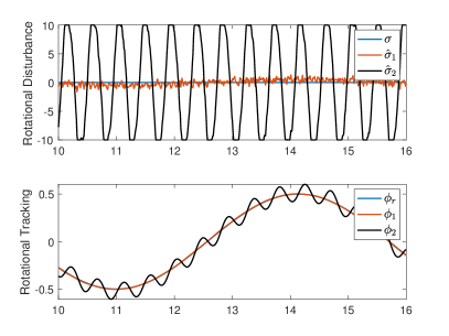
Figure 1: Simulated rotational system response with and without actuator dynamics included in the EHGO. The disturbance estimate, $\hat{\sigma}_{2}$, when actuator dynamics are omitted oscillates between the saturation bounds (top), inducing oscillations in the tracking performance of $\phi_{2}$ (bottom). The disturbance estimate, $\hat{\sigma}_{1}$, and tracking, $\phi_{1}$, show excellent performance when actuator dynamics are included in the EHGO for this example.

IV Stability Analysis

In this section, we will derive the requirements of the initial conditions that ensure that the proposed controller is well defined throughout operation. We then establish stability of the state feedback control, observer estimates, and output feedback control.

IV-A Restricting Domain of Operation

The domain of operation must be restricted in order to ensure that the rotational feedback linearizing control law remains well defined. To ensure the expressions in (16) are well-defined, we introduce the following assumption.

Assumption 3

The rotational reference signals remain in the set $\{|\phi_{r}|<\frac{\pi}{2}-\delta,|\theta_{r}|<\frac{\pi}{2}-\delta,{\color[rgb]{0,0,0}|\psi_{r}|<\frac{\pi}{2}-\delta}\}$, where $0<\delta<\frac{\pi}{2}$.

To ensure the rotational tracking error is well defined, i.e., the magnitude of each entry of $\boldsymbol{\xi}_{1}$ is smaller than $\frac{\pi}{2}$, and to ensure singularities of the Z-Y-X Euler angle representation at $\theta=\pm\frac{\pi}{2}$, the rotational states must remain in the set $\{|\phi|<\frac{\pi}{2},|\theta|<\frac{\pi}{2},{\color[rgb]{0,0,0}|\psi|<\frac{\pi}{2}},|\dot{\phi}|<a_{\theta},|\dot{\theta}|<a_{\theta},{\color[rgb]{0,0,0}|\dot{\psi}|<a_{\theta}}\}$, where $a_{\theta}$ is some positive constant. The magnitude of each entry of $\boldsymbol{\xi}_{1}$ should be smaller than $\frac{\pi}{2}$ to ensure that the rotational error is well-defined. We will now establish that for sufficiently small initial tracking error, $\boldsymbol{\xi}(0)$, the tracking error $\left\lVert\boldsymbol{\xi}_{1}(t)\right\rVert<\delta$ for all $t>0$. A Lyapunov function in the rotational error dynamics is

$$V_{\xi}=\boldsymbol{\xi}^{\top}P_{\xi}\boldsymbol{\xi},\quad\text{where}\ P_{\xi}A_{\xi}+A_{\xi}^{\top}P_{\xi}=-I_{6},$$ (27)

$$A_{\xi}=\left[\begin{smallmatrix}0_{3}&I_{3}\\ -\beta_{1}I_{3}&-\beta_{2}I_{3}\end{smallmatrix}\right].$$

A Lyapunov function in the translational error dynamics is

$$V_{\rho}=\boldsymbol{\rho}^{\top}P_{\rho}\boldsymbol{\rho},\quad\text{where}\ P_{\rho}A_{\rho}+A_{\rho}^{\top}P_{\rho}=-I_{6},$$ (28)

$$A_{\rho}=\left[\begin{smallmatrix}0_{3}&I_{3}\\ -\gamma_{1}I_{3}&-\gamma_{2}I_{3}\end{smallmatrix}\right].$$

Solving $P_{\xi}A_{\xi}+A_{\xi}^{\top}P_{\xi}=-I_{6}$ for $P_{\xi}$ and $P_{\rho}A_{\rho}+A_{\rho}^{\top}P_{\rho}=-I_{6}$ for $P_{\rho}$ yields

$$P_{\xi}=\left[\begin{smallmatrix}\frac{\beta_{1}^{2}+\beta_{1}+\beta_{2}^{2}}{2\beta_{1}\beta_{2}}I_{3}&\frac{1}{2\beta_{1}}I_{3}\\ \frac{1}{2\beta_{1}}I_{3}&\frac{\beta_{1}+1}{2\beta_{1}\beta_{2}}I_{3}\end{smallmatrix}\right],\quad P_{\rho}=\left[\begin{smallmatrix}\frac{\gamma_{1}^{2}+\gamma_{1}+\gamma_{2}^{2}}{2\gamma_{1}\gamma_{2}}I_{3}&\frac{1}{2\gamma_{1}}I_{3}\\ \frac{1}{2\gamma_{1}}I_{3}&\frac{\gamma_{1}+1}{2\gamma_{1}\gamma_{2}}I_{3}\end{smallmatrix}\right].$$

Let $c_{\xi}\in\mathbb{R}_{>0}$ be chosen such that $c_{\xi}<(\beta_{1}+1)\delta^{2}/(2\beta_{2})$, and let $\Omega_{\xi}=\{V_{\xi}<c_{\xi}\}$. Since $\boldsymbol{e}_{\vartheta}(t,\boldsymbol{\xi}_{1})$ and its partial derivatives are continuous on $\Omega_{\xi}$, and $\boldsymbol{e}_{\vartheta}$ is uniformly bounded in time, it is locally Lipschitz in $\Omega_{\xi}$ and let $L_{e}$ be the associated Lipschitz constant. Take $c_{\rho}>\lambda_{\text{max}}(P_{\rho})(2L_{e}\delta\lambda_{\text{max}}(P_{\rho}))^{2}$, where $\lambda_{\text{max}}(\cdot)$ is the maximum eigenvalue of the argument, and let $\Omega_{\rho}=\{V_{\rho}<c_{\rho}\}$. Define the domain of operation $\Omega_{q}=\Omega_{\xi}\times\Omega_{\rho}$.

Lemma 1 (Restricting Domain of Operation)

For the feedback linearized rotational error dynamics (12) with initial conditions $\boldsymbol{\xi}(0)\in\Omega_{\xi}$ the system state $\boldsymbol{\xi}(t)$ remains in the set $\left\lVert\boldsymbol{\xi}_{1}(t)\right\rVert<\delta$ for all $t>0$. Similarly, the feedback linearized translational error dynamics (17) with initial conditions $\boldsymbol{\rho}(0)\in\Omega_{\rho}$, the system state $\boldsymbol{\rho}(t)$ remains in $\Omega_{\rho}$, for all $t>0$.

Proof:

See Appendix -A. ∎

Remark 2

By Lemma 1 and Assumption 3, the rotational states remain in the set $\{|\phi|<\frac{\pi}{2},|\theta|<\frac{\pi}{2},|\dot{\phi}|<a_{\theta},|\dot{\theta}|<a_{\theta}\}$, where $a_{\theta}$ is some positive constant. Thereby ensuring singularities in the Euler angles are avoided and the feedback linearizing controllers (11) and (16) remain well defined.

Furthermore, we will restrict the domain of operation of the reference system by defining the set $\Omega_{x_{c}}=\{\|\boldsymbol{x}_{c_{1}}\|<a_{1},\|\boldsymbol{x}_{c_{2}}\|<a_{2},\|\boldsymbol{x}_{c_{3}}\|<a_{3}\}$ for $a_{1},a_{2},a_{3}\in\mathbb{R}_{>0}$.

IV-B Stability Under State Feedback

Theorem 1 (Stability Under State Feedback)

For the closed-loop state feedback rotational and translational subsystems, (12) and (17), if the initial conditions $(\boldsymbol{\xi}(0),\boldsymbol{\rho}(0))\in\Omega_{q}$, the system states $(\boldsymbol{\xi}(t),\boldsymbol{\rho}(t))\in\Omega_{q}$ for all $t>0$. Additionally, the states will exponentially converge to the origin.

Proof:

See Appendix -C. ∎

IV-C Convergence of Observer Estimates

The scaled error dynamics of the EHGO are written by making the following change of variables

$$\begin{gathered}{\eta}_{j}^{i}=\frac{({\chi}_{j}^{i}-\hat{{\chi}}_{j}^{i})}{\epsilon^{\varrho_{i}-j}},\quad\tilde{\boldsymbol{\omega}}_{s}=\boldsymbol{\omega}_{s}-\hat{\boldsymbol{\omega}}_{s},\end{gathered}$$ (29)

where $\chi_{j}^{i}$ is the $j$-th element of $\boldsymbol{\chi}_{i}$ for $1\leq i\leq 3$ and $1\leq j\leq\varrho_{i}$, and ${\hat{\chi}_{j}^{i}}$ is the estimate of $\chi_{j}^{i}$ obtained using the EGHO. In the new variables, the scaled EHGO estimation error dynamics become

$$\begin{split}\epsilon\dot{\boldsymbol{\eta}}^{i}&=F_{i}\boldsymbol{\eta}^{i}+B_{1}^{i}\left[\Delta\bar{f}^{i}+\bar{G}^{i}(\boldsymbol{\vartheta}_{1})\tilde{\boldsymbol{\omega}}_{s}\right]+\epsilon B_{2}^{i}\varphi^{i}(t,\boldsymbol{q},\boldsymbol{x}_{c}),\end{split}$$ (30)

where

$$F_{i}=\left[\begin{smallmatrix}{-\alpha_{1}^{i}}I_{3}&{I_{3}}&{\cdots}&{0_{3}}\\ {\vdots}&{}&{\ddots}&{\vdots}\\ {-\alpha^{i}_{\varrho_{i}-1}}I_{3}&{0_{3}}&{\cdots}&{I_{3}}\\ {-\alpha^{i}_{\varrho_{i}}}I_{3}&{0_{3}}&{\cdots}&{0_{3}}\end{smallmatrix}\right],\quad B_{1}^{i}=\left[\begin{smallmatrix}0_{3}\\ \vdots\\ I_{3}\\ 0_{3}\end{smallmatrix}\right],$$

$$B_{2}^{i}=\left[0_{3}\ \cdots\ 0_{3}\ I_{3}\right]^{\top},\quad\boldsymbol{\eta}^{i}=\left[{\boldsymbol{\eta}_{1}^{i}}^{\top}\ \cdots\ {\boldsymbol{\eta}_{\varrho_{i}}^{i}}^{\top}\right]^{\top},$$

and $\Delta\bar{f}^{i}=\bar{f}^{i}({\color[rgb]{0,0,0}\boldsymbol{\xi},\boldsymbol{x}_{c_{3}}},\boldsymbol{\vartheta}_{1},\dot{\bar{\boldsymbol{\vartheta}}}_{r})-\bar{f}^{i}({\color[rgb]{0,0,0}\hat{\boldsymbol{\xi}},\hat{\boldsymbol{x}}_{c_{3}}},\boldsymbol{\vartheta}_{1},\dot{\bar{\boldsymbol{\vartheta}}}_{r})$ and $\bar{f}^{i}$, $\bar{G}^{i}$, and $\varphi^{i}$ correspond to rows $3i-2$ to $3i$ of $\bar{f}$, $\bar{G}$, and $\varphi$, respectively. Note (30) is an $O(\epsilon)$ perturbation of

$$\epsilon\dot{\boldsymbol{\eta}}^{i}=F_{i}\boldsymbol{\eta}^{i}+B_{1}^{i}\left[\Delta\bar{f}^{i}+\bar{G}^{i}(\boldsymbol{\vartheta}_{1})\tilde{\boldsymbol{\omega}}_{s}\right].$$ (31)

The actuator error dynamics in terms of the error in squared rotor angular rate, $\tilde{\boldsymbol{\omega}}_{s}$, and rotor angular rate error, $\tilde{\boldsymbol{\omega}}=\boldsymbol{\omega}-\hat{\boldsymbol{\omega}}$ can be written as

$$\begin{split}\tau_{m}\dot{\tilde{\boldsymbol{\omega}}}_{s}&=-2\tilde{\boldsymbol{\omega}}_{s}+2W_{\text{des}}\tilde{\boldsymbol{\omega}},\\ \tau_{m}\dot{\tilde{\boldsymbol{\omega}}}&=-\tilde{\boldsymbol{\omega}},\end{split}$$ (32)

where $W_{\text{des}}=\text{diag}[\sqrt{\omega_{sd_{i}}}]\in\mathbb{R}^{n\times n}$ for $i\in\{1,\dots,n\}$ is time-varying. By exploiting the fact that $W_{\text{des}}$ is bounded, i.e., $\sqrt{\omega_{sd_{i}}}\leq\omega_{\max}$, for each i, where $\omega_{\max}\in\mathbb{R}$ is the maximum achievable rotor angular rate, the actuator error dynamics (32) can be analyzed as a cascaded system with the Lyapunov functions

$$V_{\tilde{\omega}_{s}}=\tilde{\boldsymbol{\omega}}_{s}^{\top}\tilde{\boldsymbol{\omega}}_{s},\quad V_{\tilde{\omega}}=\tilde{\boldsymbol{\omega}}^{\top}\tilde{\boldsymbol{\omega}},$$ (33)

and the composite Lyapunov function

$$V_{\omega}=d_{2}V_{\tilde{\omega}_{s}}+V_{\tilde{\omega}},\quad d_{2}>0,$$ (34)

where $d_{2}$ is sufficiently small (see Appendix -B for details). Define the set $\Omega_{\omega}=\{V_{\omega}\leq c_{\omega}\}$ where $c_{\omega}\in\mathbb{R}_{>0}$ is an arbitrary constant.

Lemma 2 (Stability of Actuator Dynamics)

For bounded input, $\sqrt{\boldsymbol{\omega}_{sd_{i}}}$ for $i\in\{1,\dots,n\}$, the actuator error dynamics (32) will globally exponentially converge to the origin. Therefore, the simulated rotor angular rates, $\hat{\boldsymbol{\omega}}$, exponentially converge to the actual rotor angular rates, $\boldsymbol{\omega}$.

Proof:

See Appendix -D. ∎

The systems (31) and (32) form the cascaded system

$$\begin{split}\epsilon\dot{\boldsymbol{\eta}}^{i}&=F_{i}\boldsymbol{\eta}^{i}+B_{1}^{i}\left[\Delta\bar{f}^{i}+\bar{G}^{i}(\boldsymbol{\vartheta}_{1})\tilde{\boldsymbol{\omega}}_{s}\right],\\ \tau_{m}\dot{\tilde{\boldsymbol{\omega}}}_{s}&=-2\tilde{\boldsymbol{\omega}}_{s}+2W_{\text{des}}\tilde{\boldsymbol{\omega}},\\ \tau_{m}\dot{\tilde{\boldsymbol{\omega}}}&=-\tilde{\boldsymbol{\omega}}.\end{split}$$ (35)

We now define the state vector of scaled observer error and actuator error as $\boldsymbol{\Delta}=[\boldsymbol{\eta}^{1}\;\boldsymbol{\eta}^{2}\;\boldsymbol{\eta}^{3}\;\tilde{\boldsymbol{\omega}}_{s}\;\tilde{\boldsymbol{\omega}}]^{\top}$. In comparison with a standard EHGO, (35) has additional vanishing perturbation terms with associated dynamics. In the following theorem, we establish that these perturbation terms do not affect the convergence of the EHGO. Furthermore, the perturbation term in (30) is continuous and can be bounded by $\epsilon\varphi(t,\boldsymbol{q},\boldsymbol{x}_{c})\leq\epsilon\kappa$ for $\kappa\in\mathbb{R}_{>0}$, and can be treated as a nonvanishing perturbation. Using [38, Lemma 9.2], it can be shown that the perturbed observer error dynamics converge to an $O(\epsilon\kappa)$ neighborhood of the origin.

A Lyapunov function for the EHGO error system (31) with the input, $\tilde{\boldsymbol{\omega}}_{s}$, set to zero is

$$\epsilon V_{\eta}=\sum_{i=1}^{3}(\boldsymbol{\eta}^{i})^{\top}P_{\eta}^{i}\boldsymbol{\eta}^{i},\quad P_{\eta}^{i}F_{i}+F_{i}^{\top}P_{\eta}^{i}=-I_{3\varrho_{i}}.$$ (36)

A composite Lyapunov function for (35) is

$$V_{\Delta}=d_{3}V_{\eta}+V_{\omega},\quad d_{3}>0,$$ (37)

where $d_{3}$ is sufficiently small (see Appendix -B for details).

Recall that $(\chi_{1}^{2},\chi_{2}^{2})=(\xi_{1},\xi_{2})$. Also, the estimates of $(\xi_{1},\xi_{2})$ can be expressed as $\hat{\xi}_{1}=\xi_{1}-\epsilon^{2}\eta^{2}_{1}$ and $\hat{\xi}_{2}=\xi_{2}-\epsilon\eta^{2}_{2}.$ Consider a strict subset of $\Omega_{\xi}$, defined by $\Omega^{\textup{sub}}_{\xi}\subset\Omega_{\xi}$. Define

$$\Omega_{\eta}=\{(\boldsymbol{\eta}^{1},\boldsymbol{\eta}^{2},\boldsymbol{\eta}^{3})\in\mathbb{R}^{10}\;|\;(\hat{\xi}_{1},\hat{\xi}_{2})\in\Omega_{\xi},\;\forall\boldsymbol{\xi}\in\Omega^{\textup{sub}}_{\xi}\}.$$

Let $c_{\Delta}\in\mathbb{R}_{>0}$ be the largest constant such that $\Omega_{\Delta}=\{V_{\Delta}\leq c_{\Delta}\}$ is contained in $\Omega_{\eta}\times\Omega_{\omega}$.

Theorem 2 (Convergence of EHGO Estimates)

There exists sufficiently small $\epsilon^{*}$ such that for all $\epsilon\in(0,\epsilon^{*})$, $\Omega_{\Delta}$ is positively invariant, and for each $\boldsymbol{\Delta}(0)\in\Omega_{\Delta}$, $\boldsymbol{\Delta}(t)$ converges exponentially to an $O(\epsilon\kappa)$ neighborhood of the origin.

Proof:

See Appendix -E. ∎

IV-D Stability Under Output Feedback

The system under output feedback is a singularly perturbed system which can be split into two time-scales. The multi-rotor dynamics and control reside in the slow time-scale while the observer and actuator dynamics reside in the fast time-scale. We now establish the stability of the overall output feedback system.

Theorem 3 (Stability Under Output Feedback)

For the output feedback system defined by (4), (6), (10), (21), (24), (25), and (26), the following statements hold

1. given any compact subset $\Omega_{A}\subset\Omega_{q}\times\Omega_{\Delta}$, there exists a sufficiently small $\epsilon^{*}$ such that for any $\epsilon\in(0,\epsilon^{*})$, $\Omega_{A}$ is a positively invariant set;

2. for $\epsilon\in(0,\epsilon^{*})$ the trajectories of the output feedback system exponentially converge to an $O(\epsilon\kappa)$ neighborhood of the origin with $\Omega_{A}$ as a subset of its region of attraction.

Proof:

See Appendix -F. ∎

V Numerical Simulation

The proposed method is simulated with the reference system taken as a moving ground vehicle on which the multi-rotor will land. However, since the multi-rotor may initially be far from the ground vehicle, i.e., $\boldsymbol{p}_{1}-\boldsymbol{x}_{c_{1}}$ may be large, we will bound the estimate of this error to prevent overly aggressive maneuvers by saturating $\hat{\boldsymbol{\rho}}_{1}$ as

$$\hat{\boldsymbol{\rho}}_{1_{s}}=\delta_{\rho}\operatorname{tanh}(\hat{\boldsymbol{\rho}}_{1}/\delta_{p}),$$ (38)

where $\delta_{\rho}\in\mathbb{R}$ is chosen to determine the rate of convergence of the multi-rotor position, $\boldsymbol{p}_{1}$, and the ground vehicle position, $\boldsymbol{x}_{c_{1}}$. The saturated estimate is then used in the output feedback control (25). The controller (25) using $\hat{\boldsymbol{\rho}}_{1_{s}}$ loses exponential stability outside a certain region around the origin. This can be avoided by scheduling the proportional gain, $\gamma_{1}$, in (25). However, saturation is a more natural choice and our simulations suggested that it yields superior performance.

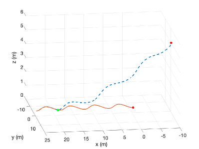
Figure 2: The trajectory of the multi-rotor UAV (dashed) and the trajectory of the ground vehicle (solid). The red points are the initial conditions and the green point signifies the occurrence of the landing.

The initial position of the multi-rotor is $\boldsymbol{p}_{1}(0)=[-10,\ 1,\ -5]^{\top}$ and the initial position of the ground vehicle is $\boldsymbol{x}_{c_{1}}(0)=[2,\ 0,\ -0.5]^{\top}$. The ground vehicle follows the trajectory $\boldsymbol{x}_{c_{1}}(t)=[t,\ 2\cos(t),\ -0.5]^{\top}$. While only having a position measurement of the ground vehicle, with added noise, the multi-rotor is able to track and land on the vehicle, as shown in Fig. 2. The multi-rotor is able to make this landing while canceling disturbances in both the rotational and translational subsystems, $\boldsymbol{\sigma}_{\xi}=[\sin(t)\ \cos(t)\ \sin(t)]^{\top}$ and $\boldsymbol{\sigma}_{\rho}=[\cos(t)\ \sin(t)\ \cos(t)]^{\top}$, respectively. Gaussian white noise is added to all measurement signals.

VI Experimental Validation

The proposed estimation and control method is implemented on an experimental platform to validate performance and show the practical application of this control methodology to landing a multi-rotor on a small moving ground vehicle.

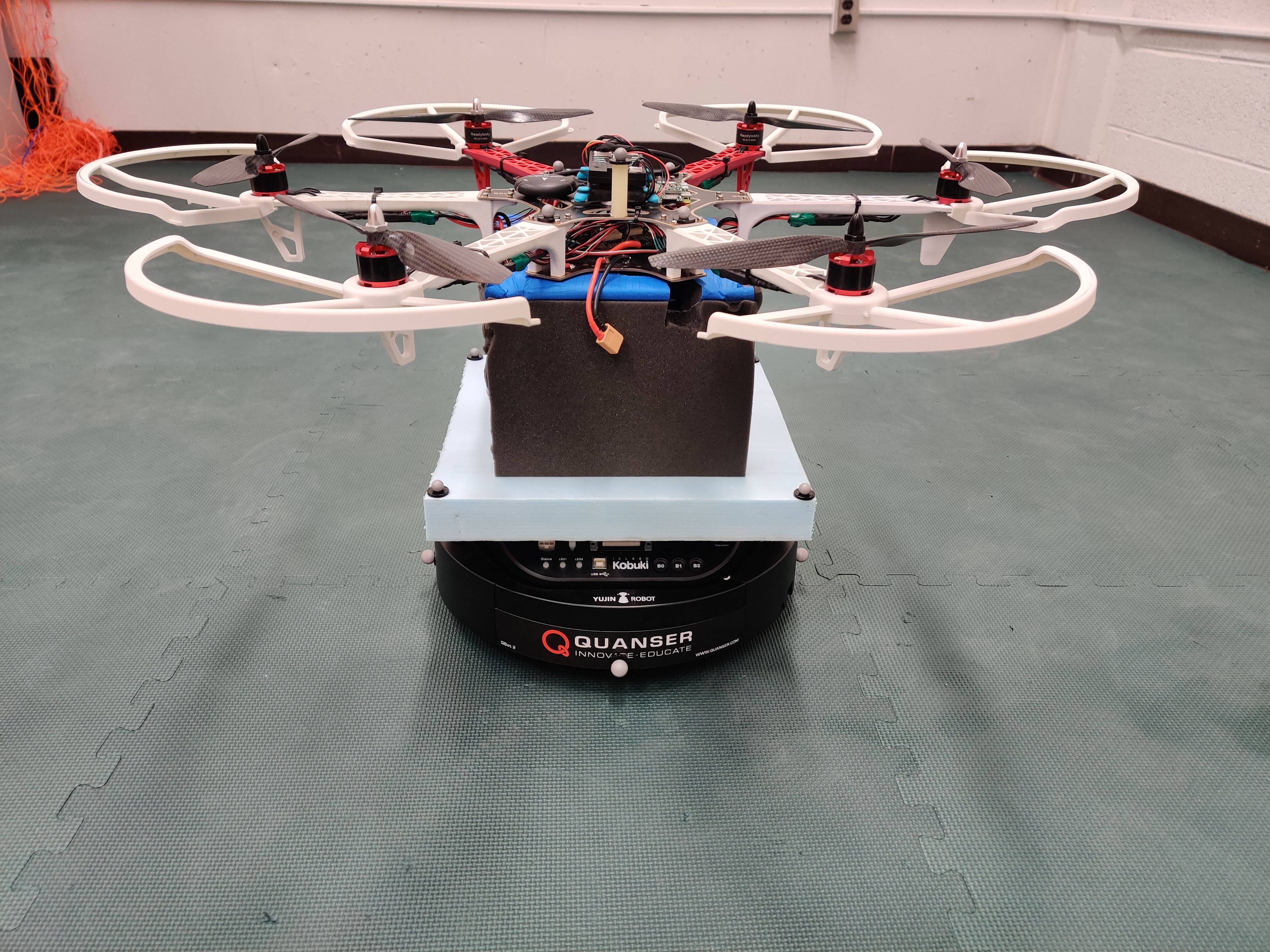
Figure 3: Experimental multi-rotor on ground vehicle landing platform.

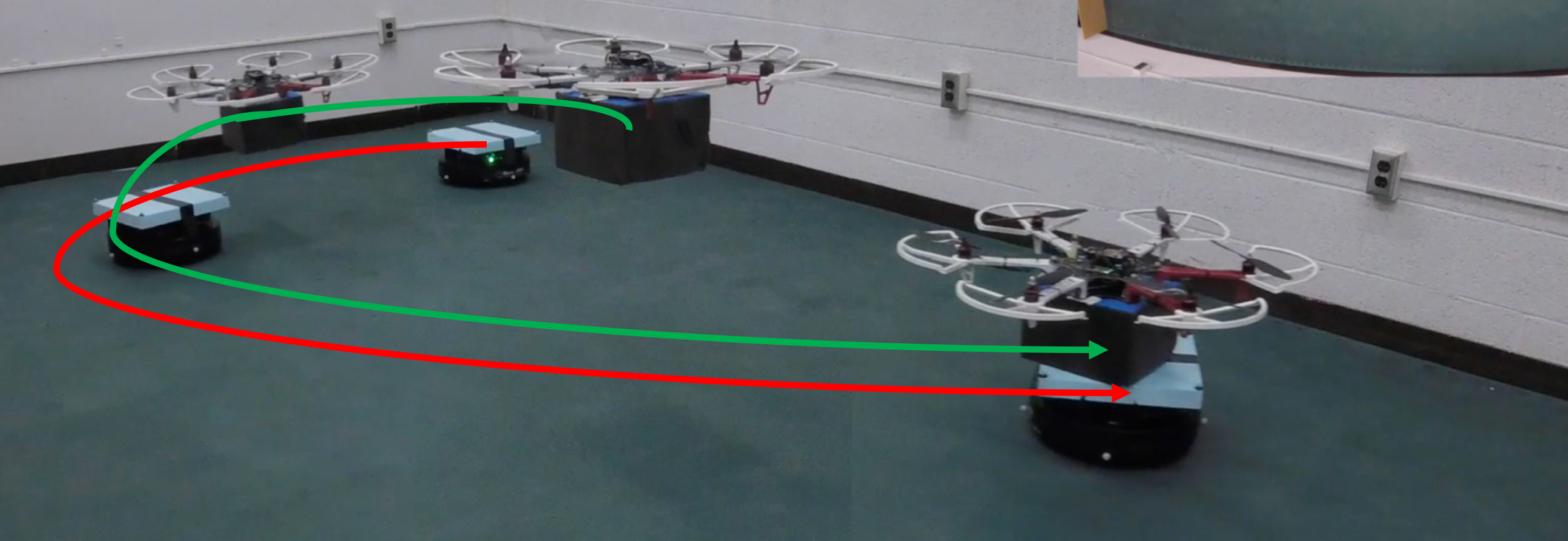
Figure 4: Experimental landing on moving ground vehicle.

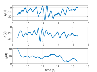
Figure 5: Estimates of the total rotational disturbance affecting the hexrotor during an experimental flight.

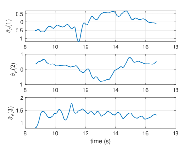
Figure 6: Estimates of the total translational disturbance affecting the hexrotor during an experimental flight.

VI-A Hardware

The experimental multi-rotor platform is built on a 550mm hexrotor frame with 920kV motors and 10x4.5 carbon fiber rotors. Six 30A electronic speed controllers (ESCs) are used for motor control and the system is powered by a 5000mAh 4s LiPo battery. The model parameters for the experimental platform were found to be

$$\begin{gathered}J=\text{diag}(0.0228\;0.0241\;0.0446),\quad m=1.824kg,\\ M=\left[\begin{smallmatrix}1&1&1&1&1&1\\ -\frac{r}{2}&-r&-\frac{r}{2}&\frac{r}{2}&r&\frac{r}{2}\\ \frac{r\sqrt{3}}{2}&0&-\frac{r\sqrt{3}}{2}&-\frac{r\sqrt{3}}{2}&0&\frac{r\sqrt{3}}{2}\\ c&-c&c&-c&c&-c\end{smallmatrix}\right],\quad c=0.1,\\ \quad b=1.8182e-05,\quad r=0.275m,\quad\tau_{m}=0.059.\end{gathered}$$

The moment of inertia matrix, $J$, was measured using the bifilar pendulum approach [39]. The mapping matrix, $M$, is derived from the geometry of the airframe, in this case a hexrotor with x geometry with rotors numbered clockwise starting from the front right. The aerodynamic drag of the rotors, $c$, and the constant mapping squared actuator speed to force, $b$, were obtained using a photo-tachometer to measure rotor angular rate and a load cell to measure the forces generated at a range of speeds. Similarly, the actuator time constant, $\tau_{m}$, was measured by applying several step inputs of varying magnitude to the rotor, measuring the response with the photo-tachometer, and fitting a first-order system to the data.

The control method is implemented on a Pixhawk 4 Flight Management Unit (FMU) in discrete time at 100Hz using Mathworks Simulink through the PX4 Autopilots Support from Embedded Coder package. This enables the control method to be integrated with the PX4 firmware to run on the Pixhawk 4 hardware. As a result, we can access fused estimates of the vehicle orientation from the EKF running in the PX4 firmware. The position estimates of both the multi-rotor and ground vehicle are pulled from a Vicon server at 100Hz. The estimates are sent over a UDP connection to a Raspberry Pi Zero that is running onboard the multi-rotor. The Raspberry Pi Zero then relays the position information to the FMU over a serial connection.

The ground vehicle is a Quanser QBot2 with a landing platform attached as shown with the multi-rotor on the landing platform in Fig. 3. The ground vehicle is manually teleoperated using a joystick through Simulink. This ensures that no prior information about the trajectory is known, as the trajectory is generated in real-time by the operator.

VI-B Experimental Procedure

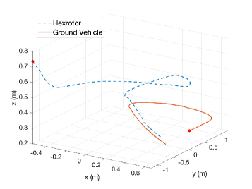
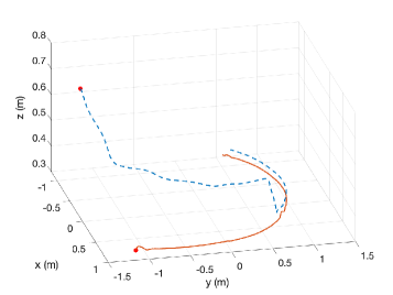
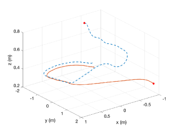
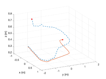
Figure 7: Multiple experimental landing trajectories showing the multi-rotor trajectory (dashed) and the ground vehicle trajectory (solid). The red dots correspond to the initial conditions of the system when a landing was commanded.

The hexrotor initially ascends to a fixed altitude and holds position until commanded to track and land on the ground vehicle. Once a landing command is sent, the hexrotor begins converging on the position of the ground vehicle while the ground vehicle is being manually teleoperated around the area until the hexrotor successfully lands.

To ensure the large initial position error does not result in overly aggressive control action, the same bounding function (38) is used to bound the position error vector $\boldsymbol{\rho}_{1}$. Furthermore, to ensure the multi-rotor approaches the ground vehicle from above, an offset is added to the $z$ component of the reference system. Once the multi-rotor is within some pre-defined radius of the center of the ground vehicle, in this case $4cm$, the offset is removed so the hexrotor will commence landing on the ground vehicle.

Multiple experimental test flights were conducted with different initial conditions for both the hexrotor and ground vehicle. Each test was also performed with different ground vehicle trajectories. These experiments show the ability of the algorithm to successfully land regardless of differences in initial conditions or different reference trajectories.

The ground vehicle trajectories and the hexrotor trajectories are shown for four different experimental flights in Fig. 7. The estimates of the disturbances affecting the system in the rotational and translational dynamics for one such flight are shown in Fig. 5 and Fig. 6, respectively. Notice that the translational disturbance estimate, specifically $\hat{\boldsymbol{\sigma}}_{\rho}(3)$ in Fig. 6, contains a constant offset. This offset is a result of the charge state of the battery. As the battery voltage decreases, the thrust applied by the rotors for a given commanded speed decreases. Also, large rotational disturbances arise in Fig. 5, which can be caused by unmodeled aerodynamic effects, inaccuracies in the inertia matrix, or differences between speed controllers. We do not model these discrepancies, however, the observer is able to estimate and compensate for these uncertainties in the control to result in excellent tracking performance. A video of the experiments can be found at https://youtu.be/oWcl4ydNLDs

VII Conclusions and Future Directions

We studied a real-time trajectory estimation and tracking problem for a multi-rotor in the presence of modeling error and external disturbances. The unknown trajectory is generated from a dynamical system with unknown or partially known dynamics. We designed and rigorously analyzed an EHGO-based output feedback controller to guarantee stable operation of the overall system.

The capability of the controller is illustrated using the example of a multi-rotor landing on a moving ground vehicle. The multi-rotor landing is shown in simulation with noise and disturbances added, as well as implemented experimentally on a hexrotor platform. Multiple initial conditions and unknown trajectories are tested experimentally and shown to result in successful landings.

We plan to extend this work to enable in-flight recovery from an actuator failure using multiple models and a family of EHGOs. This method can also be extended to consider control optimality. The feedback linearizing control could be replaced with an optimal control strategy, such as model predictive control. Furthermore, the estimates of disturbance from the EHGO could be used to parameterize a disturbance model online for use in control design.

VIII Acknowledgements

We would like to thank Professor Hassan K. Khalil for his invaluable insights on extended high-gain observer design and analysis.

-A Proof of Lemma 1 (Restricting Domain of Operation)

Substituting $P_{\xi}$ in (27), the rotational tracking error Lyapunov function can be written as

$$\small V_{\xi}=\frac{(\beta_{1}+1)\boldsymbol{\xi}_{1}^{\top}\boldsymbol{\xi}_{1}}{2\beta_{2}}+\frac{\beta_{1}\boldsymbol{\xi}_{2}^{\top}\boldsymbol{\xi}_{2}+(\beta_{2}\boldsymbol{\xi}_{1}+\boldsymbol{\xi}_{2})^{\top}(\beta_{2}\boldsymbol{\xi}_{1}+\boldsymbol{\xi}_{2})}{2\beta_{1}\beta_{2}}.$$

Taking the bound on the Lyapunov function

$$V_{\xi}\leq c_{\xi}\Rightarrow\frac{(\beta_{1}+1)\boldsymbol{\xi}_{1}^{\top}\boldsymbol{\xi}_{1}}{2\beta_{2}}\leq c_{\xi},$$

and choosing $c_{\xi}$ in the following manner

$$c_{\xi}<\frac{(\beta_{1}+1)\delta^{2}}{2\beta_{2}}\Rightarrow\left\lVert\boldsymbol{\xi}_{1}(t)\right\rVert<\delta,$$

over the set $\Omega_{\xi}$. The Lyapunov function (27) also satisfies the following inequalities

$$\lambda_{\min}(P_{\xi})\left\lVert\boldsymbol{\xi}\right\rVert^{2}\leq V_{\xi}\leq\lambda_{\max}(P_{\xi})\left\lVert\boldsymbol{\xi}\right\rVert^{2},\quad\dot{V}_{\xi}\leq-\left\lVert\boldsymbol{\xi}\right\rVert^{2},$$

where $\lambda_{\text{min}}(\cdot)$ is the minimum eigenvalue of the argument, showing that $\Omega_{\xi}$ is positively invariant.

In view of potential rotational tracking errors, the translational tracking error Lyapunov function (28) satisfies the following inequalities

$$\begin{gathered}\lambda_{\min}(P_{\rho})\left\lVert\boldsymbol{\rho}\right\rVert^{2}\leq V_{\rho}\leq\lambda_{\max}(P_{\rho})\left\lVert\boldsymbol{\rho}\right\rVert^{2},\\ \dot{V}_{\rho}\leq-\left\lVert\boldsymbol{\rho}\right\rVert^{2}+2[0_{3\times 1}\;e_{\vartheta}(t,\boldsymbol{\xi}_{1})^{\top}]^{\top}P_{\rho}\boldsymbol{\rho}.\end{gathered}$$

Since $e_{\vartheta}(t,\boldsymbol{\xi}_{1})$ and its partial derivatives are continuous on $\Omega_{\xi}$, and $e_{\vartheta}$ is uniformly bounded in time, $e_{\vartheta}$ is Lipschitz in $\boldsymbol{\xi}_{1}$ on $\Omega_{\xi}$. We can now define

$$\left\lVert e_{\vartheta}(t,\boldsymbol{\xi}_{1})-e_{\vartheta}(t,0)\right\rVert\leq L_{e}\left\lVert\boldsymbol{\xi}_{1}\right\rVert\leq L_{e}\delta,$$

for the Lipschitz constant, $L_{e}$. We can then bound the translational Lyapunov function derivative by

$$\dot{V}_{\rho}\leq-\left\lVert\boldsymbol{\rho}\right\rVert^{2}+2L_{e}\delta\lambda_{\text{max}}(P_{\rho})\left\lVert\boldsymbol{\rho}\right\rVert.$$

For $\left\lVert\boldsymbol{\rho}\right\rVert>2L_{e}\delta\lambda_{\text{max}}(P_{\rho})$, $\dot{V}_{\rho}<0$. Since $V_{\rho}\leq\lambda_{\text{max}}(P_{\rho})\left\lVert\boldsymbol{\rho}\right\rVert^{2}$ we can choose

$$c_{\rho}>\lambda_{\text{max}}(P_{\rho})(2L_{e}\delta\lambda_{\text{max}}(P_{\rho}))^{2}.$$ (39)

By this choice, $\dot{V}_{\rho}<0$ for $V_{\rho}\geq c_{\rho}$, hence $\Omega_{\rho}$ is compact and positively invariant. Thus, the domain of operation $\Omega_{q}=\Omega_{\xi}\times\Omega_{\rho}$ is positively invariant. $\hfill\blacksquare$

-B Stability of Generalized Cascade Systems

A generalized stability proof for cascade systems is adapted from Appendix C.1 of [40]. Consider the cascade connection of two systems

$$\dot{\eta}=f_{1}(t,\eta,\xi),\quad\dot{\xi}=f_{2}(\xi),$$ (40)

where $f_{1}$ and $f_{2}$ are locally Lipschitz and $f_{1}(t,0,0)=0$, $f_{2}(0)=0$. Assuming the origin of $\dot{\xi}=f_{2}(\xi)$ is exponentially stable, there is a continuously differentiable Lyapunov function, $V_{2}(\xi)$, that satisfies the following inequalities

$$c_{1}\left\lVert\xi\right\rVert^{2}\leq V_{2}(\xi)\leq c_{2}\left\lVert\xi\right\rVert^{2},$$ (41a)

$$\quad\frac{\partial V_{2}(\xi)}{\partial\xi}f_{2}(\xi)\leq-c_{3}\left\lVert\xi\right\rVert^{2},$$ (41b)

$$\left\lVert\frac{\partial V_{2}(\xi)}{\partial\xi}\right\rVert\leq c_{4}\left\lVert\xi\right\rVert,$$ (41c)

over the set $\Omega_{2}=\{V_{2}(\xi)<c_{5}\}$ for some $c_{5}\in\mathbb{R}_{>0}$.

Now, suppose there is a continuously differentiable Lyapunov function, $V_{1}(\eta)$, that satisfies the inequalities

$$\frac{\partial V_{1}(\eta)}{\partial\eta}f_{1}(t,\eta,0)\leq-c\left\lVert\eta\right\rVert^{2},\quad\left\lVert\frac{\partial V_{1}(\eta)}{\partial\eta}\right\rVert\leq k\left\lVert\eta\right\rVert,$$ (42)

over the set $\Omega_{1}=\{V_{1}(\eta)<c_{6}\}$ for some $c_{6}\in\mathbb{R}_{>0}$.

Take a composite Lyapunov function for the cascaded system as

$$V(\eta,\xi)=bV_{1}(\eta)+V_{2}(\xi),\quad b>0,$$ (43)

in which $b$ can be arbitrarily chosen. The derivative, $\dot{V}$, satisfies

$$\begin{split}\dot{V}(\eta,\xi)&=b\frac{\partial V_{1}(\eta)}{\partial\eta}f_{1}(t,\eta,0)+\\ &b\frac{\partial V_{1}(\eta)}{\partial\eta}\left[f_{1}(t,\eta,\xi)-f_{1}(t,\eta,0)\right]+\frac{\partial V_{2}(\xi)}{\partial\xi}f_{2}(\xi),\\ \dot{V}(\eta,\xi)&\leq-bc\left\lVert\eta\right\rVert^{2}+bkL\left\lVert\eta\right\rVert\left\lVert\xi\right\rVert-c_{3}\left\lVert\xi\right\rVert^{2},\end{split}$$

where $f_{1}$ is Lipschitz in $\xi$ on $\Omega_{2}$, and $L$ is the associated Lipschitz constant.

The inequality can be written in quadratic form as

$$\begin{split}\dot{V}(\eta,\xi)&\leq-\left[\begin{matrix}\left\lVert\eta\right\rVert\\ \left\lVert\xi\right\rVert\end{matrix}\right]^{\top}\left[\begin{matrix}bc&\frac{-bkL}{2}\\ \frac{-bkL}{2}&c_{3}\end{matrix}\right]\left[\begin{matrix}\left\lVert\eta\right\rVert\\ \left\lVert\xi\right\rVert\end{matrix}\right],\\ &=-\left[\begin{matrix}\left\lVert\eta\right\rVert\\ \left\lVert\xi\right\rVert\end{matrix}\right]^{\top}Q\left[\begin{matrix}\left\lVert\eta\right\rVert\\ \left\lVert\xi\right\rVert\end{matrix}\right]\leq-\lambda_{\min}(Q)\left\lVert\left[\begin{matrix}\left\lVert\eta\right\rVert\\ \left\lVert\xi\right\rVert\end{matrix}\right]\right\rVert^{2},\end{split}$$

where $b$ is chosen such that $b<4cc_{3}/(kL)^{2}$ to ensure $Q$ is positive definite. The foregoing analysis shows that the origin of (40) is exponentially stable on the set $\Omega=\Omega_{1}\times\Omega_{2}$.

-C Proof of Theorem 1 (Stability Under State Feedback)

The translational and rotational closed-loop systems can be written as a cascaded system in the following form

$$\begin{aligned} \dot{\boldsymbol{\rho}}_{1}&=\boldsymbol{\rho}_{2},\\ \dot{\boldsymbol{\rho}}_{2}&=-\gamma_{1}\boldsymbol{\rho}_{1}-\gamma_{2}\boldsymbol{\rho}_{2}+\boldsymbol{e}_{\vartheta}(t,\boldsymbol{\xi}_{1}),\\ \dot{\boldsymbol{\xi}}_{1}&=\boldsymbol{\xi}_{2},\\ \dot{\boldsymbol{\xi}}_{2}&=-\beta_{1}\boldsymbol{\xi}_{1}-\beta_{2}\boldsymbol{\xi}_{2},\end{aligned}\ \Rightarrow\ \begin{aligned} \dot{\boldsymbol{\rho}}_{1}&=\boldsymbol{\rho}_{2},\\ \dot{\boldsymbol{\rho}}_{2}&=f_{1}(t,\boldsymbol{\rho},\boldsymbol{\xi}),\\ \dot{\boldsymbol{\xi}}_{1}&=\boldsymbol{\xi}_{2},\\ \dot{\boldsymbol{\xi}}_{2}&=f_{2}(\boldsymbol{\xi}).\end{aligned}$$

Taking the Lyapunov functions for the rotational and translational subsystems, (27) and (28), a composite Lyapunov function can be written

$$V_{sf}=d_{1}V_{\rho}+V_{\xi},\quad d_{1}>0.$$ (44)

Since $V_{\rho}$ satisfies (42) on $\Omega_{\rho}$, $V_{\xi}$ satisfies (41) on $\Omega_{\xi}$, and $f_{1}(t,\boldsymbol{\rho},\boldsymbol{\xi})$ is Lipshitz in $\boldsymbol{\xi}$ on $\Omega_{\xi}$, it can be shown following the generalized proof in Appendix -B that for $d_{1}$ small enough, the entire closed-loop state feedback system converges exponentially to the origin for any trajectory starting within the domain of operation, $\Omega_{q}$. $\hfill\blacksquare$

-D Proof of Lemma 2 (Stability of Actuator Dynamics)

The Lyapunov functions for the actuator dynamics (32) are $V_{\tilde{\omega}_{s}}$ and $V_{\tilde{\omega}}$ from (33), with the composite Lyapunov function (34). Since $V_{\tilde{\omega}_{s}}$ satisfies (42) globally, $V_{\tilde{\omega}}$ satisfies (41) globally, and $\dot{\tilde{\boldsymbol{\omega}}}_{s}$ is globally Lipschitz in $\tilde{\boldsymbol{\omega}}$ since $W_{\text{des}}$ is bounded, using the general result for cascaded systems in Appendix -B, it can be shown that the origin is globally exponentially stable when $d_{2}$ is chosen small enough. $\hfill\blacksquare$

-E Proof of Theorem 2 (Convergence of EHGO Estimates)

The Lyapunov function for the actuator error system is (34) and the Lyapunov function for the EHGO error system with the input, $\tilde{\boldsymbol{\omega}}_{s}$, set to zero is (36). A composite Lyapunov function for the cascaded system (35) is (37). The function $\bar{f}^{i}({\color[rgb]{0,0,0}\boldsymbol{\xi},\boldsymbol{x}_{c_{3}}},\boldsymbol{\vartheta}_{1},\dot{\bar{\boldsymbol{\vartheta}}}_{r})$ is Lipschitz in $\boldsymbol{\xi}$ and $\boldsymbol{x}_{c_{3}}$ on $\Omega_{\xi}\times\Omega_{x_{c}}$ and $(\hat{\xi}_{1},\hat{\xi}_{2})\in\Omega_{\xi}$. Thus, $\Delta\bar{f}^{i}$ can be bounded by

$$\left\lVert\Delta\bar{f}^{i}\right\rVert\leq L_{\eta}\left\lVert\boldsymbol{\chi}_{i}-\hat{\boldsymbol{\chi}}_{i}\right\rVert\Rightarrow\left\lVert\Delta\bar{f}^{i}\right\rVert\leq\epsilon L_{\eta}\left\lVert\boldsymbol{\eta}^{i}\right\rVert,$$

leading to the following bound on the derivative of the Lyapunov function

$$\begin{split}\epsilon\dot{V}_{\eta}&\leq\sum_{i=1}^{3}\left(-\left\lVert\boldsymbol{\eta}^{i}\right\rVert^{2}+2\epsilon L_{\eta}\left\lVert\boldsymbol{\eta}^{i}\right\rVert^{2}\left\lVert P_{\eta}^{i}B_{1}^{i}\right\rVert\right),\\ \epsilon\dot{V}_{\eta}&\leq-\left\lVert\boldsymbol{\eta}\right\rVert^{2}+2\epsilon L_{\eta}\left\lVert N\right\rVert\left\lVert\boldsymbol{\eta}\right\rVert^{2},\end{split}$$

where the elements of the diagonal matrix $N$ are $N_{i}=\left\lVert P_{\eta}^{i}B_{1}^{i}\right\rVert$. Since $\alpha_{j}^{i}$ are tunable and $\epsilon$ is a design parameter, pick $\epsilon$ such that $2\epsilon L_{\eta}\left\lVert N\right\rVert\leq\frac{1}{2}$ resulting in the following inequality

$$\epsilon\dot{V}_{\eta}\leq-\frac{1}{2}\left\lVert\boldsymbol{\eta}\right\rVert^{2}.$$ (45)

The composite Lyapunov function (37) consists of $V_{\eta}$ and $V_{\omega}$, where $V_{\eta}$ satisfies (42) on $\Omega_{\eta}$, $V_{\omega}$ satisfies (41) on $\Omega_{\omega}$, and $\epsilon\dot{\boldsymbol{\eta}}$ is Lipschitz in $\tilde{\boldsymbol{\omega}}_{s}$ on $\Omega_{\omega}$. Following Appendix -B, the origin of (35) is exponentially stable for any trajectory starting in $\Omega_{\Delta}$. Furthermore, the cascade connection of the complete scaled observer error system (30) and the actuator error dynamics (32) is the same as (35) with perturbation. The perturbation is bounded by $\epsilon\varphi(t,\boldsymbol{q},\boldsymbol{x}_{c})<\epsilon\kappa$ and is continuous, therefore it can be treated as a nonvanishing perturbation. Following [38, Lemma 9.2], the estimation error of the EHGO converges exponentially to an $O(\epsilon\kappa)$ neighborhood of the origin. Furthermore, $\Omega_{\Delta}$ will remain invariant under the nonvanishing perturbation. $\hfill\blacksquare$

-F Proof of Theorem 3 (Stability Under Output Feedback)

The existence of sufficiently small $\epsilon^{*}$ such that $\Omega_{A}$ is invariant can be established analogously to [38, Theorem 14.6]. The entire output feedback closed-loop system can now be written in singularly perturbed form

$$\dot{\boldsymbol{q}} =A_{c}\boldsymbol{q}+\Delta(\boldsymbol{\eta}),$$ (46a)

$$\epsilon\dot{\boldsymbol{\eta}}^{i} =F_{i}\boldsymbol{\eta}^{i}+B_{1}^{i}\left[\Delta\bar{f}^{i}+\bar{G}^{i}(\boldsymbol{\vartheta}_{1})\tilde{\boldsymbol{\omega}}_{s}\right]+\epsilon B_{2}^{i}\varphi^{i}(t,\boldsymbol{q},\boldsymbol{x}_{c}),$$ (46b)

$$\tau_{m}\dot{\tilde{\boldsymbol{\omega}}}_{s} =-2\tilde{\boldsymbol{\omega}}_{s}+2W_{\text{des}}\tilde{\boldsymbol{\omega}},$$ (46c)

$$\tau_{m}\dot{\tilde{\boldsymbol{\omega}}} =-\tilde{\boldsymbol{\omega}},$$ (46d)

where

$$A_{c}=\left[\begin{smallmatrix}A_{\rho}&0_{6}\\ 0_{6}&A_{\xi}\end{smallmatrix}\right].$$

The term $\Delta(\boldsymbol{\eta})$ is due to estimation errors and is $O(\epsilon\kappa)$ and can be defined by

$$\Delta(\boldsymbol{\eta})=\left[\begin{smallmatrix}0_{3\times 1}\\ \gamma_{1}\epsilon^{2}\boldsymbol{\eta}_{1}^{1}+\gamma_{2}\epsilon\boldsymbol{\eta}_{2}^{1}+\boldsymbol{\eta}_{3}^{1}-\boldsymbol{\eta}_{3}^{3}\\ 0_{3\times 1}\\ \beta_{1}\epsilon^{2}\boldsymbol{\eta}_{1}^{2}+\beta_{2}\epsilon\boldsymbol{\eta}_{2}^{2}+\boldsymbol{\eta}_{3}^{2}+\epsilon L_{\eta}\left\lVert\boldsymbol{\eta}_{2}^{2}\right\rVert\end{smallmatrix}\right].$$

First, we ignore the last term, $\epsilon B^{i}\varphi^{i}(t,\boldsymbol{q},\boldsymbol{x}_{c})$, in the $\boldsymbol{\eta}$ dynamics. In this case, the closed-loop system has a two-time-scale structure because $\epsilon$ and $\tau_{m}$ are small. Since the effect of $\Delta(\boldsymbol{\eta})$ in (46a) vanishes as $\epsilon$ is pushed to zero, the boundary layer system can be taken as (46b)–(46d) and the slow dynamics can be taken as (46a). From Theorem 2, the origin of the boundary layer system is an exponentially stable equilibrium point as $\epsilon\to 0$, and from Theorem 1, the origin of the slow system is an exponentially stable equilibrium point.

With the inclusion of $\epsilon B^{i}\varphi^{i}(t,\boldsymbol{q},\boldsymbol{x}_{c})$ in the $\boldsymbol{\eta}$ dynamics, the overall system is an $O(\epsilon k)$ perturbation of an exponentially stable system. Therefore, similar to [38, Lemma 9.2], it can be shown that the entire closed-loop system with output feedback control (46) will converge to an $O(\epsilon\kappa)$ neighborhood of the origin for any trajectory starting in $\Omega_{q}\times\Omega_{\Delta}$. $\hfill\blacksquare$

-G Peaking Phenomenon

The EHGO estimation error $\tilde{\chi}_{i}=\chi_{i}-\hat{\chi}_{i}$ can be bounded by

$$|\tilde{\chi}_{i}|\leq\frac{b}{\epsilon^{\varrho-1}}\left\lVert\boldsymbol{\tilde{\chi}}(0)\right\rVert e^{-at/\epsilon},$$ (47)

for some positive constants $a$ and $b$, by Theorem 2.1 in [41]. Initially, the estimation error can be very large, i.e., $O(1/\epsilon^{\varrho-1})$, but will decay rapidly. To prevent the peaking of the estimates from entering the plant during the initial transient, the output feedback controller needs to be saturated. This is done by saturating the individual estimates outside a compact set of interest using (23).

There is some set $\{V_{\eta}\leq\epsilon^{2}c\}$ for some $c\in\mathbb{R}_{>0}$ that the estimation error will enter after some short time, $T(\epsilon)$, where $\lim_{\epsilon\rightarrow 0}T(\epsilon)=0$. Since the initial state $\boldsymbol{q}(0)$ resides on the interior of the modified compact set of Theorem 3, $\Omega_{A}$, choosing $\epsilon$ small enough will ensure that $\boldsymbol{q}$ will not leave $\Omega_{A}$ during the interval $[0,T(\epsilon)]$. This establishes the boundedness of all states.

References

• [1] C. J. Boss, V. Srivastava, and H. K. Khalil, “Robust tracking of an unknown trajectory with a multi-rotor UAV: A high-gain observer approach,” in American Control Conference, (Denver, CO), pp. 1429–1434, July 2020. Extended version available at: arXiv preprint arXiv:2003.06390.
• [2] C. Papachristos, T. Dang, S. Khattak, F. Mascarich, N. Khedekar, and K. Alexis, “Modeling, control, state estimation and path planning methods for autonomous multirotor aerial robots,” Foundations and Trends in Robotics, vol. 7, no. 3, pp. 180–250, 2018.
• [3] V. Kumar and N. Michael, “Opportunities and challenges with autonomous micro aerial vehicles,” The International Journal of Robotics Research, vol. 31, no. 11, pp. 1279–1291, 2012.
• [4] D. Tzoumanikas, Q. Yan, and S. Leutenegger, “Nonlinear MPC with motor failure identification and recovery for safe and aggressive multicopter flight,” in International Conference on Robotics and Automation (ICRA), pp. 8538–8544, 2020.
• [5] D. Mellinger, N. Michael, and V. Kumar, “Trajectory generation and control for precise aggressive maneuvers with quadrotors,” The International Journal of Robotics Research, vol. 31, no. 5, pp. 664–674, 2012.
• [6] H. Huang, G. M. Hoffmann, S. L. Waslander, and C. J. Tomlin, “Aerodynamics and control of autonomous quadrotor helicopters in aggressive maneuvering,” in International Conference on Robotics and Automation, pp. 3277–3282, IEEE, 2009.
• [7] Z. Fang and W. Gao, “Adaptive integral backstepping control of a micro-quadrotor,” in International Conference on Intelligent Control and Information Processing, vol. 2, pp. 910–915, IEEE, 2011.
• [8] M. Huang, B. Xian, C. Diao, K. Yang, and Y. Feng, “Adaptive tracking control of underactuated quadrotor unmanned aerial vehicles via backstepping,” in American Control Conference, pp. 2076–2081, IEEE, 2010.
• [9] A. Mokhtari, A. Benallegue, and B. Daachi, “Robust feedback linearization and GH controller for a quadrotor unmanned aerial vehicle,” in International Conference on Intelligent Robots and Systems, pp. 1198–1203, IEEE, 2005.
• [10] D. Lee, C. Nataraj, T. C. Burg, and D. M. Dawson, “Adaptive tracking control of an underactuated aerial vehicle,” in American Control Conference, pp. 2326–2331, IEEE, 2011.
• [11] D. Brescianini and R. D’Andrea, “Computationally efficient trajectory generation for fully actuated multirotor vehicles,” IEEE Transactions on Robotics, vol. 34, no. 3, pp. 555–571, 2018.
• [12] Y. Li, H. Eslamiat, N. Wang, Z. Zhao, A. K. Sanyal, and Q. Qiu, “Autonomous waypoints planning and trajectory generation for multi-rotor UAVs,” in Proceedings of the Workshop on Design Automation for CPS and IoT, pp. 31–40, 2019.
• [13] M. W. Mueller, M. Hehn, and R. D’Andrea, “A computationally efficient motion primitive for quadrocopter trajectory generation,” IEEE Transactions on Robotics, vol. 31, no. 6, pp. 1294–1310, 2015.
• [14] T. Sangyam, P. Laohapiengsak, W. Chongcharoen, and I. Nilkhamhang, “Autonomous path tracking and disturbance force rejection of UAV using fuzzy based auto-tuning PID controller,” in International Conference on Electrical Engineering/Electronics, Computer, Telecommunications and Information Technology, pp. 528–531, IEEE, 2010.
• [15] H. Voos, “Nonlinear control of a quadrotor micro-UAV using feedback-linearization,” in International Conference on Mechatronics, pp. 1–6, IEEE, 2009.
• [16] D. Lee, H. J. Kim, and S. Sastry, “Feedback linearization vs. adaptive sliding mode control for a quadrotor helicopter,” International Journal of Control, Automation and Systems, vol. 7, no. 3, pp. 419–428, 2009.
• [17] V. K. Chitrakaran, D. M. Dawson, J. Chen, and M. Feemster, “Vision assisted autonomous landing of an unmanned aerial vehicle.,” in Conference on Decision and Control, pp. 1465–1470, IEEE, 2005.
• [18] T. Madani and A. Benallegue, “Backstepping control with exact 2-sliding mode estimation for a quadrotor unmanned aerial vehicle,” in International Conference on Intelligent Robots and Systems, pp. 141–146, IEEE, 2007.
• [19] C. Diao, B. Xian, Q. Yin, W. Zeng, H. Li, and Y. Yang, “A nonlinear adaptive control approach for quadrotor UAVs,” in Asian Control Conference (ASCC), pp. 223–228, IEEE, 2011.
• [20] P. Bouffard, A. Aswani, and C. Tomlin, “Learning-based model predictive control on a quadrotor: Onboard implementation and experimental results,” in International Conference on Robotics and Automation, pp. 279–284, IEEE, 2012.
• [21] H. L. N. N. Thanh and S. K. Hong, “Quadcopter robust adaptive second order sliding mode control based on PID sliding surface,” IEEE Access, vol. 6, pp. 66850–66860, 2018.
• [22] S. Kim, S. Choi, H. Kim, J. Shin, H. Shim, and H. J. Kim, “Robust control of an equipment-added multirotor using disturbance observer,” Transactions on Control Systems Technology, vol. 26, no. 4, pp. 1524–1531, 2018.
• [23] W. Kong, D. Zhou, D. Zhang, and J. Zhang, “Vision-based autonomous landing system for unmanned aerial vehicle: A survey,” in International Conference on Multisensor Fusion & Information integration for Intelligent Systems, pp. 1–8, 2014.
• [24] A. Gautam, P. Sujit, and S. Saripalli, “A survey of autonomous landing techniques for UAVs,” in International Conference on Unmanned Aircraft Systems, pp. 1210–1218, 2014.
• [25] Y. Feng, C. Zhang, S. Baek, S. Rawashdeh, and A. Mohammadi, “Autonomous landing of a UAV on a moving platform using model predictive control,” Drones, vol. 2, no. 4, p. 34, 2018.
• [26] J. A. Macés-Hernández, F. Defaÿ, and C. Chauffaut, “Autonomous landing of an UAV on a moving platform using model predictive control,” in Asian Control Conference, pp. 2298–2303, 2017.
• [27] B. Herissé, T. Hamel, R. Mahony, and F.-X. Russotto, “Landing a VTOL unmanned aerial vehicle on a moving platform using optical flow,” IEEE Transactions on Robotics, vol. 28, no. 1, pp. 77–89, 2011.
• [28] P. Serra, R. Cunha, T. Hamel, D. Cabecinhas, and C. Silvestre, “Landing of a quadrotor on a moving target using dynamic image-based visual servo control,” IEEE Transactions on Robotics, vol. 32, no. 6, pp. 1524–1535, 2016.
• [29] J. L. Sanchez-Lopez, J. Pestana, S. Saripalli, and P. Campoy, “An approach toward visual autonomous ship board landing of a VTOL UAV,” Journal of Intelligent & Robotic Systems, vol. 74, no. 1-2, pp. 113–127, 2014.
• [30] T. Hoang, E. Bayasgalan, Z. Wang, G. Tsechpenakis, and D. Panagou, “Vision-based target tracking and autonomous landing of a quadrotor on a ground vehicle,” in American Control Conference, pp. 5580–5585, 2017.
• [31] J. Kim, Y. Jung, D. Lee, and D. H. Shim, “Outdoor autonomous landing on a moving platform for quadrotors using an omnidirectional camera,” in International Conference on Unmanned Aircraft Systems, pp. 1243–1252, 2014.
• [32] F. Kendoul, “Four-dimensional guidance and control of movement using time-to-contact: Application to automated docking and landing of unmanned rotorcraft systems,” The International Journal of Robotics Research, vol. 33, no. 2, pp. 237–267, 2014.
• [33] T. Lee, M. Leok, and N. H. McClamroch, “Geometric tracking control of a quadrotor UAV on SE(3),” in Conference on Decision and Control, pp. 5420–5425, IEEE, 2010.
• [34] A. Franchi and A. Mallet, “Adaptive closed-loop speed control of BLDC motors with applications to multi-rotor aerial vehicles,” in International Conference on Robotics and Automation (ICRA), pp. 5203–5208, IEEE, 2017.
• [35] J. Lee, R. Mukherjee, and H. K. Khalil, “Control design for a helicopter using dynamic inversion and extended high gain observers,” in ASME Dynamic Systems and Control Conference, pp. 653–660, 2012.
• [36] J. Lee, R. Mukherjee, and H. K. Khalil, “Output feedback performance recovery in the presence of uncertainties,” Systems & Control Letters, vol. 90, pp. 31–37, 2016.
• [37] C. J. Boss, J. Lee, and J. Choi, “Uncertainty and disturbance estimation for quadrotor control using extended high-gain observers: Experimental implementation,” in ASME Dynamic Systems and Control Conference, pp. V002T01A003–V002T01A003, 2017.
• [38] H. K. Khalil, Nonlinear Systems. Upper Saddle River, 2002.
• [39] M. Jardin and E. Mueller, “Optimized measurements of UAV mass moment of inertia with a bifilar pendulum,” in AIAA Guidance, Navigation and Control Conference, p. 6822, 2007.
• [40] H. K. Khalil, Nonlinear Control. Pearson New York, 2015.
• [41] H. K. Khalil, High-Gain Observers in Nonlinear Feedback Control. Society for Industrial and Applied Mathematics, 2017.