Cosmological constraints of interacting phantom dark energy models

Abstract

In this paper, we consider three phantom dark energy models, in the context of interaction between the dark components namely cold dark matter (CDM) and dark energy (DE). The first model, known as $w_{\textrm{d}}$CDM can induce a big rip singularity (BR) while the two remaining induce future abrupt events known as the Little Rip (LR) and Little Sibling of the Big Rip (LSBR). These phantom DE models can be distinguished by their equation of state. We invoke a new phenomenon such as the interaction between CDM and DE given that it could solve or alleviate some of the problems encountered in standard cosmology. We aim to find out the effect of such an interaction on the cosmological parameters of the studied models, as well as, the persistence or the disappearance of the singularity and the abrupt events induced by the models under study. We choose an interaction term proportional to DE density, i.e. $Q=\lambda H\rho_{\textrm{d}}$, since the case where $Q\propto\rho_{\textrm{m}}$ could lead to a large scale instability at early time. We also do not claim at all that $Q=\lambda H\rho_{\textrm{d}}$ is the ideal choice since it suffers from a negative CDM density in the future. By the use of a Markov Chain Monte Carlo (MCMC) approach, and by assuming a flat FLRW Universe, we constrain the cosmological parameters of each of the three phantom DE models studied. Furthermore, by the aid of the corrected Akaike Information Criterion ($\text{AIC}_{c}$) tool, we compare our phantom DE models. Finally, a perturbative analysis of phantom DE models under consideration is performed based on the best fit background parameters.

I INTRODUCTION

The observations of distant type Ia supernovae (SNIa), the Cosmic Microwave Background measurements (CMB) and the Baryon acoustic Oscillations (BAO) Riess:1998cb ; Perlmutter:1998np ; Ade:2015rim indicate that the expansion of the Universe is presently accelerating. The origin behind this acceleration is still a mystery up to date. One of the most accepted explanations to this phenomenon is the suggestion that the Universe is filled with a dark component known as dark energy (DE). The most popular model up to now to explain accurately the data is $\Lambda$CDM, where $\Lambda$ is the cosmological constant and it plays the role of dark energy. Even though, $\Lambda$CDM explains the observational data almost on all scales, it suffers from many problems, such as the coincidence problem Cai:2004dk , the age problem caused by old quasars Duran:2010ky . Over the years, while researchers suggested many models that are basically extensions of $\Lambda$CDM model in the context of general relativity for different types of scalar fields, like quintessence Ratra:1987rm , k-essence ArmendarizPicon:2000ah or for different kind of equations of state such as the Chaplygin gas Kamenshchik:2001cp , other extensions based on modified theories of gravity like f(R)-gravity Sotiriou:2008rp ; DeFelice:2010aj , f(T)-gravity Ferraro:2006jd ; Ferraro:2008ey ; Bengochea:2008gz and f(R,T)-gravity Harko:2011kv ; Nojiri:2004bi ; Allemandi:2005qs ; Nojiri:2006gh ; Nojiri:2009kx have been also proposed as an alternative mechanism to describe the current acceleration of the Universe. In this paper, we will focus on the first aforementioned class of DE.

Our knowledge about the dark components and their features is still very limited, since they are only detected indirectly via their gravitational effects, which makes their nature very secretive. One of the innovative ideas in modern cosmology is to consider an interaction between the dark components i.e. CDM and DE, which allows an energy transfer between them. Suggesting DE models that include new effects like interaction between DE and CDM will provide not only the possibility to investigate the dark sector on a completely new level, but also could help us to discriminate between different theoretical models. Furthermore, such interactions could help to solve or alleviate the standard cosmology problems cited above.

The discovery that our Universe is accelerating has motivated theorists to infer the best theoretical model from observations. As a result, hundreds of theoretical models have been proposed to this aim based on different theories. Some of these models present singularities i.e. cosmological quantities that go to infinity at a finite cosmic time, while others present abrupt events, i.e. cosmological quantities that diverge at an infinite cosmic time. The equation of state (EoS) of DE models which is the ratio between the pressure and the energy density can lead to different fates of the Universe. In general, we can classify DE models in two classes: the first class corresponds to an EoS larger than -1, this type of models is known as quintessence, the second class corresponds to models having an EoS smaller than -1 and are known as phantom models. Surprisingly, and even though they violate the null energy condition, these models are the most supported by cosmological observations Aghanim:2018eyx ; Caldwell:1999ew ; Jimenez:2016sgs ; Sahni:2014ooa ; Vagnozzi:2018jhn ; Alam:2016wpf rather than being ruled out as it was expected. In the current paper, we will focus on three phantom DE models, that induce different doomsday known as Big Rip (BR) Caldwell:1999ew ; Dabrowski:2003jm ; Starobinsky:1999yw ; Caldwell:2003vq ; Carroll:2003st ; Chimento:2003qy ; GonzalezDiaz:2003rf ; GonzalezDiaz:2004vq ; Sahni:2002dx Little Rip (LR) Ruzmaikina ; Bouhmadi-Lopez:2013nma ; Nojiri:2005sx ; Nojiri:2005sr ; Stefancic:2004kb ; BouhmadiLopez:2005gk ; Frampton:2011sp ; Brevik:2011mm ; Contreras:2018two and Little Sibling of the Big Rip (LSBR) Bouhmadi-Lopez:2014cca ; Morais:2016bev ; Morais:2016bev ; Bouhmadi-Lopez:2018lly .

In absence of interaction between DE and CDM the BR model induces a true singularity while the two remnants induce a future abrupt events. In a previous work Bouali:2019whr ; Albarran:2016mdu , we have studied the same set of models without interaction between DE and CDM components, the analysis was done at the background and the perturbative levels by means of a Markov Chain Monte Carlo (MCMC) at the background level Sagredo:2018ahx . In the current paper, we study the same models by taking into account an interaction between DE and CDM in order to find out how the exchange of energy density between the dark components could modify the models suitability according to observations. Furthermore, it may enhances the statistical evidence of the models, in particular, as compared to $\Lambda$CDM. In addition, general relativity could describe the background dynamics of the Universe even when such kind of interactions is taken into account. The interaction between CDM and DE densities is usually introduced phenomenologically given the absence of a theory determining the choice of such form. Among the years many forms have been tested such as $Q=3\lambda H\rho_{\textrm{m}}$, $Q=3\lambda H\rho_{\textrm{d}}$ and $Q=3\lambda H\frac{\rho_{\textrm{d}}\rho_{\textrm{m}}}{\rho_{\textrm{d}}+\rho_{\textrm{m}}}$ among others Amendola:1999qq ; Billyard:2000bh ; Zimdahl:2001ar ; Farrar:2003uw ; Chimento:2003iea ; Olivares:2005tb ; Koivisto:2005nr ; Sadjadi:2006qp ; Guo:2007zk ; Zhang:2007uh ; Boehmer:2008av ; Pereira:2008at ; He:2010ta ; Li:2011ga ; Clemson:2011an ; Xu:2013jma ; Cheng:2019bkh ; epjc2018 ; ijmp2020 . In this paper, we consider the following interaction $Q=\lambda H\rho_{\textrm{d}}$, where a positive coupling $\lambda>0$ ensures an energy transfer from CDM to DE density, while a negative coupling $\lambda<0$ ensures an energy transfer from DE to CDM density. Thus, the continuity equations are written as follows:

$$\left\{\begin{array}[]{l}\dot{\rho}_{\textrm{m}}+3H\rho_{\textrm{m}}=-Q,\\ \dot{\rho}_{\textrm{d}}+3H(1+w_{\textrm{d}})\rho_{\textrm{d}}=Q,\end{array}\right.$$ (1)

where $\rho_{\textrm{m}}$, $\rho_{\textrm{d}}$ and $\lambda$ are the CDM, DE energies densities and the strength of the interaction, respectively, where for simplicity we choose $Q=\lambda H\rho_{\textrm{d}}$. The standard form of the dimensionless Friedmann equation is

$$E(a)^{2}=\Omega_{\textrm{r}}+\Omega_{\textrm{m}}+\Omega_{\textrm{d}},$$ (2)

where $E(a)=H/H_{0}$ and

$$\Omega_{\textrm{r}}=\frac{8\pi G}{3H_{0}^{2}}\rho_{\textrm{r}},\;\Omega_{\textrm{m}}=\frac{8\pi G}{3H_{0}^{2}}\rho_{\textrm{m}}\;\text{and}\;\Omega_{\textrm{d}}=\frac{8\pi G}{3H_{0}^{2}}\rho_{\textrm{d}},$$ (3)

are the fractional energy densities of radiation, CDM and DE, respectively. From now on, the subindex $0$ will stand for values fixed at present, therefore, $\Omega_{\textrm{r0}}+\Omega_{\textrm{m0}}+\Omega_{\textrm{d0}}=1$ is satisfied.

The combination of observational probes we use to constraint our phantom DE models are the Pantheon compilation of SNIa dataset Scolnic:2017caz , Planck 2018 distance priors of CMB Zhai:2018vmm ; Aghanim:2018eyx , BAO measurements including 6dFGS, SDSS DR7 MGS, BOSS-LOWZ, BOSS-DR12, WiggleZ, BOSS-CMASS, Lya and DES Anderson:2013zyy ; Beutler:2011hx ; Ross:2014qpa ; Kazin:2014qga ; Alam:2016hwk and the direct measurements of the Hubble parameter Anderson:2013zyy ; Zhang:2012mp ; Stern:2009ep ; Moresco:2012jh ; Chuang:2012qt ; Moresco:2015cya ; Moresco:2016mzx ; Stocker:2018avm . After extracting the best fit parameters and their corresponding minimal $\chi^{2}$ values, we classify our models according to their ability to fit the observational data by using the so called Akaike Information Criterion ($\text{AIC}_{c}$), the results of this analysis are summarised in table 2.

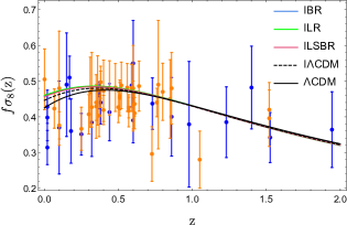
Figure 6: This plot shows the evolution of the predicted $f\sigma_{8}$ of IBR, ILR, ILSBR and $\Lambda$CDM model against the observational growth rate data shown in table 5 . The black curve corresponds to the $\Lambda$CDM, while the light blue, the green and the pink curves correspond to IBR, ILR and ILSBR models, respectively. The blue points correspond to RSD-22 compilation while the remaining points of RSD-63 are plotted in orange color.

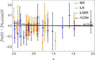
Figure 7: This plot shows the difference of the predicted $f\sigma_{8}$ of IBR, ILR and ILSBR model with respect to that of the $\Lambda$CDM. The black curve corresponds to the $\Lambda$CDM, while the light blue, the green and the pink curve correspond to IBR, ILR and ILSBR models, respectively. The blue points correspond to RSD-22 compilation while the remaining points of RSD-63 are plotted in orange color.

The paper is structured as follows: in Section II we review the induced singularities and abrupt events without interaction for a generalised EoS which unifies the models addressed in the present work. In section III we give a short description of the three phantom DE models studied in this work and the observational constraints through the MCMC confidence contours for each of them. In section IV, we analyse the asymptotic behaviour of $\dot{H}$ in order to classify the induced future abrupt event when considering interaction between DE and CDM. In section V, we present the MCMC results in the table 2, we show also the evolution of the EoS of these three models with respect to that of $\Lambda$CDM. Section VI is dedicated to the first order perturbation analysis where the results are shown in table 4. We show also in the same section (see figures 6 and 7) the theoretical predictions of $f\sigma_{8}$ for each models, and compare them with those corresponding to $\Lambda$CDM. Finally, section VII is dedicated to the conclusions.

II Non-interacting DE

In this section we analyse a generalised EoS that unifies the DE models considered in the present work, these paradigms, obey the following EoS:

• Model A: $p_{\textrm{d}}=w_{\textrm{d}}\rho_{\textrm{d}}$.

• Model B: $p_{\textrm{d}}=-\left(\rho_{\textrm{d}}+B\rho_{\textrm{d}}^{\frac{1}{2}}\right)$.

• Model C: $p_{\textrm{d}}=-\left(\rho_{\textrm{d}}+\frac{C}{3}\right).$

Therefore, we could write a generalised EoS that gathers the above mentioned models in a single equation:

$$p_{\textrm{d}}=-\left(\rho_{\textrm{d}}+A\rho_{\textrm{d}}^{\alpha}\right),$$ (4)

where the constants $A$ and $\alpha$ characterise the model. We assume a positive value for $A$ for the fluid to be a phantom type of DE. Our models A, B and C correspond to, $A=-(w_{\textrm{d}}+1),B,C/3$ and $\alpha=1,1/2,0$ respectively. We will consider a single DE component. Using the conservation equation $\dot{\rho_{\textrm{d}}}+3H\left(p_{\textrm{d}}+\rho_{\textrm{d}}\right)=0$, where dot stands for derivative with respect the cosmic time, we get:

$$\frac{d\rho_{\textrm{d}}}{da}=\frac{3A}{a}\rho_{\textrm{d}}^{\alpha}.$$ (5)

Solving the equation (5) and choosing $\rho(a_{0})=\rho_{0}$, where $a_{0}=1$, we get

$$\rho_{\textrm{d}}=\left[3A\left(1-\alpha\right)x+\rho_{\textrm{d}0}^{1-\alpha}\right]^{\frac{1}{1-\alpha}},$$ (6)

where we have defined $x\equiv\ln{(a)}$, therefore, $\dot{x}\equiv H$ and derivatives over time transform as $\dot{\left\{\phantom{a}\right\}}=H{\left\{\phantom{a}\right\}}_{x}$, where the subindex $x$ stands for derivatives over $x$. Therefore, the Hubble parameter and its cosmic time derivatives could be written as:

$$H =\left(\frac{8\pi G}{3}\right)^{\frac{1}{2}}\left[3A\left(1-\alpha\right)x+\rho_{\textrm{d}0}^{1-\alpha}\right]^{\frac{1}{2\left(1-\alpha\right)}},$$ (7)

$$\dot{H} =\left(\frac{8\pi G}{3}\right)\left(\frac{3A}{2}\right)\left[3A\left(1-\alpha\right)x+\rho_{\textrm{d}0}^{1-\alpha}\right]^{\frac{2\alpha}{2\left(1-\alpha\right)}},$$ (8)

$$\ddot{H} =\left(\frac{8\pi G}{3}\right)^{\frac{3}{2}}\left(\frac{3A}{2}\right)^{2}2\alpha\left[3A\left(1-\alpha\right)x+\rho_{\textrm{d}0}^{1-\alpha}\right]^{\frac{4\alpha-1}{2\left(1-\alpha\right)}},$$ (9)

$$\vdots$$

$$H^{(n)} =\left(\frac{8\pi G}{3}\right)^{\frac{n+1}{2}}\left(\frac{3A}{2}\right)^{n}\prod^{n-1}_{j=0}\left(2\alpha j-j+1\right)$$

$$\times\left[3A\left(1-\alpha\right)x+\rho_{\textrm{d}0}^{1-\alpha}\right]^{\frac{n\left(2\alpha-1\right)+1}{2\left(1-\alpha\right)}},$$ (10)

where $H^{(n)}$ denotes the $n^{\textrm{th}}$ derivatives of the Hubble parameter with respect to the cosmic time. Finally, we solve equation (7) to get the dependence of $x$ with respect to the cosmic time

$$x=\frac{1}{3A\left(1-\alpha\right)}\left\{\left[\left(6\pi G\right)^{\frac{1}{2}}A\left(1-2\alpha\right)(t-t_{0})\right.\right.$$

$$\left.\left.+\rho_{\textrm{d}0}^{\frac{1-2\alpha}{2}}\right]^{\frac{2\left(1-\alpha\right)}{1-2\alpha}}-\rho_{\textrm{d}0}^{\left(1-\alpha\right)}\right\}.\$$ (11)

We next analyse the phenomenology of the model (4) described by different values of $\alpha$:

• If $\alpha\leq 0$, the Hubble parameter diverges at large scales and at an infinite cosmic time but its cosmic time derivative vanishes at that point. We could identify this event as a LSBR wherein the first cosmic time derivative of the Hubble parameter vanishes at an infinite cosmic time instead of being a non-vanishing finite constant. This event is even smoother than the usual LSBR event ($\alpha=0$). We could consider the limit $\alpha\rightarrow-\infty$, in which we recover the $\Lambda$CDM paradigm, (it is equivalent to choosing $A\rightarrow 0$). In that case the Hubble parameter stands constant at large scales and the Universe approaches asymptotically a de Sitter (dS) space time.

• If $0<\alpha\leq 1/2$, first, we deduce that $H$ and $\dot{H}$ diverge at an infinite cosmic time and an infinite scale factor, therefore, this event corresponds to a LR. Second, we should distinguish between two different cases: i) if $\alpha=\alpha_{n}\equiv(n-1)/2n$, then the $n^{\textrm{th}}$ cosmic time derivative of the Hubble parameter is finite while the lower order derivatives blow up at an infinite cosmic time and an infinite scale factor. ii) if $\alpha_{n-1}<\alpha<\alpha_{n}$, then the $n^{\textrm{th}}$ derivative of $H$ vanishes while the lower order derivatives blow up at an infinite cosmic time. Hence, we deduce that between the LSBR abrupt event and the BR singularity there is a range of different LR abrupt events that could be characterised by the order in which the cosmic time derivative of Hubble parameter is finite (or vanishes). Therefore, we could coin these types of events as “$n^{\textrm{th}}$ order LR” abrupt event when $\alpha=\alpha_{n}$ and “$n^{\textrm{th}}$ zero order LR” abrupt event when $\alpha_{n-1}<\alpha<\alpha_{n}$. For example, in the “second order LR” abrupt event ($n=2,\alpha_{2}=1/4$), $H$ and $\dot{H}$ blow up at an infinite cosmic time and an infinite scale factor but the second order derivative, $\ddot{H}$, stands finite. We could move towards higher orders, where for $n\rightarrow\infty$ we get $\alpha=1/2$, that is, in the strongest version of the LR abrupt event, the Hubble parameter and all its successive cosmic time derivatives blow up at an infinite cosmic time and an infinite scale factor. We could name this event as the “infinite order LR” abrupt event.

• If $1/2<\alpha\leq 1$, the scale factor, the Hubble parameter and its cosmic time derivatives blow up at a finite cosmic time. Therefore, we identify this event with a BR.

• If $1<\alpha$, the Hubble parameter and its cosmic time derivatives blow up not only at a finite cosmic time but also at a finite scale factor as well. Therefore, we identify this event with a Big Freeze (BF).

In summary, when $\alpha\rightarrow-\infty$ we recover the cosmological constant model and the Universe is asymptotically dS. When $\alpha\leq 0$, the Universe faces a LSBR abrupt event. If $0<\alpha\leq 1/2$, the Universe faces a LR abrupt event. If $1/2<\alpha\leq 1$, the induced singularity is a BR while for $1<\alpha$ is a BF. We sumarise the discussed abrupt events and singularities in table 1.

Event	$t$	$a$	$H$	$\dot{H}$	$H^{(n)}$	$\alpha$
dS	$\infty$	$\infty$	$H_{\Lambda}$	$0$	$0$	$\alpha\rightarrow-\infty$
LSBR⋆	$\infty$	$\infty$	$\infty$	$0$	$0$	$\alpha<0$
LSBR${}^{\phantom{a}}$	$\infty$	$\infty$	$\infty$	$\dot{H}_{ls,1}$	$0$	$\alpha=0$
$n^{\textrm{th}}$ zero order LR	$\infty$	$\infty$	$\infty$	$\infty$	$0$	$\alpha_{n-1}<\alpha<\alpha_{n}$
$n^{\textrm{th}}$ order LR	$\infty$	$\infty$	$\infty$	$\infty$	$H^{(n)}_{ls,n}$	$\alpha=\alpha_{n}$
infinite order LR	$\infty$	$\infty$	$\infty$	$\infty$	$\infty$	$\alpha=1/2$
BR	$t_{br}$	$\infty$	$\infty$	$\infty$	$\infty$	$1/2<\alpha\leq 1$
BF	$t_{bf}$	$a_{bf}$	$\infty$	$\infty$	$\infty$	$1<\alpha$

Table 1: This table shows some of the features of the main cosmological events achieved with a EoS as given in Eq. (4). The first column refers to the cosmological event, the second column resumes the set of diverging cosmological parameters while the third column shows the value of $\alpha$ for which the event occurs, where $\alpha_{n}=(n-1)/2n$ for $1<n$.

We conclude that for $1/2<\alpha$, the singularity occurs at a finite cosmic time while for $1<\alpha$ it also occurs at a finite scale factor. Note that asymptotically the EoS parameter goes as $w_{\textrm{d}}\rightarrow-1$ as far as $\alpha<1$, it is constant, $w=-(1+A)$, when $\alpha=1$ and diverges for $1<\alpha$. On the other hand, we could identify the limit $\alpha\rightarrow-\infty$ with the $\Lambda$CDM paradigm. However, we emphasise that while in a LSBR abrupt event all the bound structures are unavoidably destroyed, this is not the case in a Universe dominated by a cosmological constant. The specific set of values of $\alpha$ such that the acceleration is strong enough to induce the destruction of the bound structures will involve further calculations (see, for example, section 4 in Bouhmadi-Lopez:2014cca ). At least, for $0\leq\alpha$ we expect an effective destruction of the structures to occur at a finite cosmic time Bouhmadi-Lopez:2014cca .

Finally, we trust that the values of $\alpha$ chosen to describe the three phantom DE models addressed in the present work are the most representative in their own species. First, $\alpha=0$ represents the smoother model inducing a LS where we know that the bound structures are ripped apart. Second, $\alpha=1/2$ is the particular value that induces the strongest version of a LR. Third, $\alpha=1$ is the largest value wherein a BR occurs. By the way, $\alpha=1/2$ and $\alpha=1$ are special cases which need a careful analysis. We will not consider a model inducing a BF as it leads to a singularity at a finite scale factor unlike the BR, LR, and LSBR. We will regard $\Lambda$CDM model as a guideline to compare our results. Nevertheless, we emphasise that an appropriate fitting of an interacting model should constrain the parameters $A$, $\alpha$ and $\lambda$ simultaneously rather than constraining $A$ and $\lambda$ with a previously chosen $\alpha$, as we do in the present work. The motivation of focusing on these representative models consists on understanding how the interaction affects the fate of the Universe in each case. As we will show in section IV, once the interaction between DE and DM is switched on all the abrupt events turn into a BR singularity. We emphasise that the analysis followed in this section only considers phantom models ($0<A$). Standard models, ($A<0$), would require a further analysis that will be done elsewhere.

III Interacting DM-DE

In this section we describe three phantom DE models under study. We solve the continuity equation to get the DE and CDM densities for each model. We also show their confidence contours of the MCMC analysis using the data corresponding to Bouali:2019whr .

Using the conservation equation (1) and the generalised EoS (4), the energy density of DE and CDM can be written as

$$\rho_{\textrm{d}}=\left[\left(\frac{3A}{\lambda}+\rho_{\textrm{d}0}^{1-\alpha}\right)e^{\lambda\left(1-\alpha\right)x}-\frac{3A}{\lambda}\right]^{\frac{1}{1-\alpha}},$$ (12)

$$\rho_{\textrm{m}}= D_{0}e^{-3x}-\frac{\lambda}{3}\left(-\frac{3A}{\lambda}\right)^{\frac{1}{1-\alpha}}{}_{2}F_{1}\left[\beta,\gamma,\delta,f(x)\right],$$ (13)

where $D_{0}$ is a constant such that $\rho_{\textrm{m}}(0)=\rho_{\textrm{m}0}$, where the subscript $0$ denotes present values and ${}_{2}F_{1}\left[\beta,\gamma;\delta;f(x)\right]$ is the Hypergeometric function. In addition, the parameters $\beta,\gamma,\delta$ and the argument $f(x)$ read

$$\beta \equiv\frac{1}{\alpha-1},$$ (14)

$$\gamma \equiv\frac{3}{\lambda\left(1-\alpha\right)},$$ (15)

$$\delta \equiv 1+\frac{3}{\lambda\left(1-\alpha\right)},$$ (16)

$$f(x) \equiv\left(1+\frac{\lambda}{3A}\rho_{\textrm{d}0}^{1-\alpha}\right)e^{\lambda\left(1-\alpha\right)x}.$$ (17)

We next show the results for the special cases $\alpha=1$ (model A) and $\alpha=1/2$ (model B), and we analyse as well the particular value $\alpha=0$ (model C).

III.1 MODEL A: $\alpha=1$

The model A of the present work coincides with the widely known $w_{\textrm{d}}$CDM model. Without interaction between DE and CDM its EoS reads as follows:

$$p_{\textrm{d}}=w_{\textrm{d}}\rho_{\textrm{d}}.$$ (18)

This model induces a BR singularity. When considering interaction, we use the conservation equation (1) and the EoS (18) to get the expression with respect to the scale factor of both energy densities of DE and DM,

$$\rho_{\textrm{d}}(a)=\rho_{\textrm{d0}}a^{(\lambda-3(1+w_{\textrm{d}}))},$$ (19)

$$\rho_{\textrm{m}}(a)=\left(\rho_{m0}+\frac{\lambda\rho_{\textrm{d0}}}{\lambda-3w_{\textrm{d}}}\right)a^{-3}-\frac{\lambda\rho_{\textrm{d0}}}{\lambda-3w_{\textrm{d}}}a^{(\lambda-3(1+w_{\textrm{d}}))}.$$ (20)

We label this model as IBR. The $\Lambda$CDM model can be recovered by fixing $w_{\textrm{d}}=-1$ and $\lambda=0$. The BR singularity continue to exist if the condition $3(1+w_{\textrm{d}})<\lambda$ is satisfied.

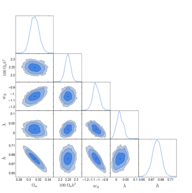
Figure 1: This figure corresponds to 1$\sigma$, 2$\sigma$ and 3$\sigma$ confidence contours obtained from SNIa+CMB+BAO+$\textrm{H}(z)$ data for the IBR model.

III.2 MODEL B: $\alpha=1/2$

The second DE model under consideration is characterised by the following EoS Nojiri:2005sx ; Stefancic:2004kb

$$p_{\textrm{d}}=-\left(\rho_{\textrm{d}}+B\rho_{\textrm{d}}^{\frac{1}{2}}\right),$$ (21)

where $B$ is a positive constant. Without interaction, it induces the abrupt event known as LR. Under interaction, the evolutions of DE and CDM densities are obtained by solving the conservation equation Eq. (1) and Eq. (21)

$$\rho_{\textrm{d}}(a)=\rho_{\textrm{d0}}\left[a^{\lambda/2}+\frac{3}{\lambda}\sqrt{\frac{\Omega_{\textrm{lr}}}{\Omega_{\textrm{d0}}}}\left(a^{\lambda/2}-1\right)\right]^{2},$$ (22)

$$\rho_{\textrm{m}}(a)= \Big{\{}\rho_{m0}+\lambda\rho_{\textrm{d0}}\Big{(}\frac{1}{\lambda+3}-\frac{6}{(\lambda+3)(\lambda+6)}\sqrt{\frac{\Omega_{\textrm{lr}}}{\Omega_{\textrm{d0}}}}-\frac{3(6-\lambda)}{\lambda^{2}(\lambda+6)}\frac{\Omega_{\textrm{lr}}}{\Omega_{\textrm{d0}}}\Big{)}\Big{\}}a^{-3}$$ (23)

$$- \frac{\lambda}{\lambda+3}\rho_{\textrm{d0}}\Big{(}1+\frac{3}{\lambda}\sqrt{\frac{\Omega_{\textrm{lr}}}{\Omega_{\textrm{d0}}}}\Big{)}^{2}a^{\lambda}+\frac{3}{\lambda+6}\rho_{\textrm{d0}}\sqrt{\frac{\Omega_{\textrm{lr}}}{\Omega_{\textrm{d0}}}}\Big{(}1+\frac{3}{\lambda}\sqrt{\frac{\Omega_{\textrm{lr}}}{\Omega_{\textrm{d0}}}}\Big{)}^{2}a^{\lambda/2}-\frac{3}{\lambda}\rho_{\textrm{d0}}{\frac{\Omega_{\textrm{lr}}}{\Omega_{\textrm{d0}}}},$$

where we have defined the dimensionless parameters $\Omega_{\textrm{lr}}$ and $\Omega_{\textrm{d0}}$ as

$$\Omega_{\textrm{lr}}=\frac{8\pi G}{3H^{2}_{0}}B^{2},\qquad\Omega_{\textrm{d0}}=\frac{8\pi G}{3H_{0}^{2}}\rho_{\textrm{d0}}.$$ (24)

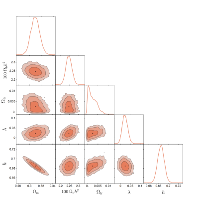
Figure 2: This figure corresponds to 1$\sigma$, 2$\sigma$ and 3$\sigma$ confidence contours obtained from SNIa+CMB+BAO+$\textrm{H}(z)$ data for the ILR model.

III.3 MODEL C: $\alpha=0$

The third model deviates from the $\Lambda$CDM’s EoS by a positive constant parameter $C/3$ as Bouhmadi-Lopez:2014cca

$$p_{\textrm{d}}=-\left(\rho_{\textrm{d}}+\frac{C}{3}\right).$$ (25)

Without interaction, this model induces the abrupt event known as LSBR. When considering interaction, we use the conservation equation (1) and Eq. (25) to obtain the evolution of DE and CDM densities

$$\rho_{\textrm{d}}(a)=\rho_{\textrm{d0}}\left(\Big{(}1+\frac{\Omega_{\textrm{lsbr}}}{\lambda\Omega_{\textrm{d0}}}\Big{)}a^{\lambda}-\frac{\Omega_{\textrm{lsbr}}}{\lambda\Omega_{\textrm{d0}}}\right),$$ (26)

$$\rho_{\textrm{m}}(a) = \left\{\rho_{m0}+\frac{\lambda\rho_{\textrm{d0}}}{\lambda+3}\left(1-\frac{\Omega_{\textrm{lsbr}}}{3\Omega_{\textrm{d0}}}\right)\right\}a^{-3}$$ (27)

$$- \frac{\lambda\rho_{\textrm{d0}}}{\lambda+3}\Big{(}1+\frac{\Omega_{\textrm{lsbr}}}{\lambda\Omega_{\textrm{d0}}}\Big{)}a^{\lambda}+\rho_{\textrm{d0}}\frac{\Omega_{\textrm{lsbr}}}{3\Omega_{\textrm{d0}}},$$

where the dimensionless quantity $\Omega_{\textrm{lsbr}}$ is related to the positive parameter $C$ as $\Omega_{\textrm{lsbr}}\equiv(8\pi G/3H_{0}^{2})C$.

IV The cosmological events induced by models under interaction

In a scenario where matter and DE are separately conserved, the models introduced in III.1, III.2 and III.3 induce the cosmological events known as BR, LR and LSBR, respectively. Nevertheless, the end of the Universe would not be the same when an interaction between matter and DE is considered. The cosmological singularities are often classified according to the divergence of some of the cosmological magnitudes, as for example, the Hubble parameter and its cosmic time derivatives Bouhmadi-Lopez:2019zvz . In addition, we refer to a singularity when it occurs at a finite cosmic time (as it is the case of BR) while we coin it as an abrupt event when it occurs at an infinite cosmic time (as it is the case of LR and LSBR) Albarran:2016mdu .

In this section, we analyse the asymptotic behaviour of the first cosmic time derivative of the Hubble parameter, $\dot{H}$, in order to appropriately classify the cosmic event induced by each model under DE and CDM interaction. Before proceeding with the calculations some comments are in order. From a first glance, the expressions for the energy density of CDM and DE (see Eqs. (19) and (20) for the model IBR, Eqs.(19) and (23) for the model ILR and Eqs. (26) and (27) for the model ILSBR) show a power law with respect to the scale factor. If the highest power of the scale factor is positive, which is indeed our case in all the interaction models considered here, the scale factor diverges at a finite cosmic time. Therefore, we are dealing with true curvature singularities rather than abrupt events.

In order to get the first cosmic time derivative of the Hubble parameter, we first derive the Friedmann equation with respect to the cosmic time,

$$2H\dot{H}=\frac{\kappa}{3}\left(\dot{\rho}_{\textrm{m}}+\dot{\rho}_{\textrm{d}}\right),$$ (28)

where $\kappa=8\pi G$. Then, we replace the conservation equation (1) to get

$$\dot{H}=-\frac{\kappa}{2}\left(\rho_{\textrm{m}}+\rho_{\textrm{d}}+p_{\textrm{d}}\right).$$ (29)

Finally, it just remains to replace the equations (18)-(27) above. We next show the asymptotic behaviour of $\dot{H}$ for the models with interaction considered in the present work.

• Model IBR

  $$\dot{H}\approx-\frac{3}{2}H_{0}^{2}\Omega_{\textrm{d}0}\left(\frac{\lambda}{\lambda-3w_{\textrm{d}}}+1+w_{\textrm{d}}\right)a^{\lambda-3\left(1+w_{\textrm{d}}\right)},$$ (30)

• Model ILR

  $$\dot{H}\approx\frac{3}{2}H_{0}^{2}\Omega_{\textrm{d}0}\frac{\lambda}{\lambda+3}\left(1+\frac{3}{\lambda}\sqrt{\frac{\Omega_{\textrm{lr}}}{\Omega_{\textrm{d}0}}}\right)^{2}a^{\lambda},$$ (31)

• Model ILSBR

  $$\dot{H}\approx\frac{3}{2}H_{0}^{2}\frac{\Omega_{\textrm{d}0}}{1+\lambda}\left(\lambda+\frac{\Omega_{\textrm{lsbr}}}{\Omega_{\textrm{d}0}}\right)a^{\lambda}.$$ (32)

We remind that the parameter $\lambda$ is positive and $\kappa\rho_{\textrm{i}0}\equiv 3\Omega_{\textrm{i}0}H_{0}^{2}$ (i=r,d,m) following the definitions given in the expression (3). As can be seen, for all the interacting scenarios considered in the present work $\dot{H}$ diverges at very large scale factors. Consequently, it follows that the induced singularities are like BR type. Surprisingly, phantom DE models in absence of interaction induce a smoother versions of the BR (LR and LSBR). However, they lead to a true BR singularity when switching on the interaction with matter.

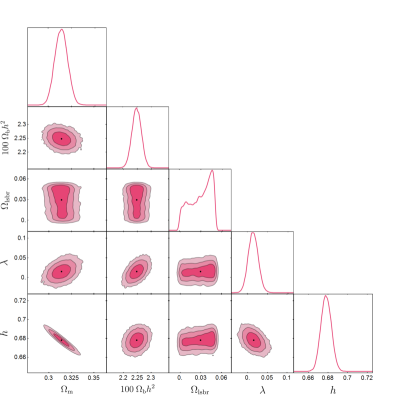
Figure 3: This figure corresponds to 1$\sigma$, 2$\sigma$ and 3$\sigma$ confidence contours obtained from SNIa+CMB+BAO+$\textrm{H}(z)$ data for the ILSBR model.

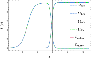
Figure 4: This figure shows the energy tranfer between CDM and DE densities. The plot shows the decaying process of CDM density into DE density. The three models IBR, ILR and ILSBR show almost a perfect overlap. The black vertical line denotes the present. We remind that $x=\ln(a)$ and $a=1$; i.e. $x=0$, at present.

V RESULTS

In order to discuss the results carried out by this analysis, we present as a first step the priors used to constrain the cosmological parameters. For all models, we have allowed matter density, the product of baryons density times the square of the Hubble rate, the Hubble rate and the strength of the interaction to vary as $\Omega_{\textrm{m}}\in\left\{0.001,0.5\right\}$, $\Omega_{\textrm{b}}h^{2}\in\left\{0.001,0.08\right\}$, $h\in\left\{0.4,1\right\}$ and $\lambda\in\left\{-1,1\right\}$, respectively . Besides the dimensionless parameters $\Omega_{lr}$ and $\Omega_{lsbr}$ vary in $\left\{0,1.7\times 10^{-3}\right\}$ and $\left\{0,5.025\times 10^{-2}\right\}$, respectively. The choice of the dimensionless parameters $\Omega_{lr}$ and $\Omega_{lsbr}$ is done to compare our interacting models with the non interacting ones Bouali:2019whr . Indeed, in the non interacting case this choice is mandatory to avoid negative values of the DE density in the past, in particular, from the beginning of our numerical integration, i.e. $a_{\textrm{ini}}=10^{-6}$. From table 2, we observe that for I$\Lambda$CDM model the amount of matter i.e. $\Omega_{\textrm{m}}$ increases, while the Hubble rate $h$ decreases slightly when compared to $\Lambda$CDM. From the confidence contours in figures 1, 2 and 3, we remark that the couple ($\omega_{\textrm{d}}$,$\lambda$) presents a negative correlation, while the couples ($\Omega_{\textrm{lr}}$,$\lambda$) and ($\Omega_{\textrm{lsbr}}$,$\lambda$) present a positive correlation. We notice as well that our results of $H_{0}$ are far away from the one given by local measurements, e.g by Riess et al Riess:2019cxk . This mismatch between the $H_{0}$ values has become very troublesome and dubbed as the $H_{0}$ tension problem. As an attempt to solve this issue, physics beyond the standard model must be advocated, for example higher number of effective relativistic species and non-zero curvature can be helpful to smooth this problem (see the interesting review DiValentino:2021izs for further information on this topic).

In order to classify the phantom DE models studied in this paper, based on their statistical ability to fit observational points, we use the corrected Akaike Information Criterion ($AIC_{c}$) defined as AIC

$$AIC_{c}=-2\ln{\cal{L}}_{max}+2k+\frac{2k(k+1)}{N_{\textrm{d}}-k-1},$$ (33)

where $k$ and $N_{\textrm{d}}$ denote the number of free parameters and the total number of observational data, respectively. For a random Gaussian distributions chi squared takes the following form

$$\chi^{2}_{min}=-2\ln{\cal{L}}_{max}.$$

The $AIC_{c}$ is a powerful tool to compare models having a different number of free parameters, as well as a different number of data. Indeed, the model corresponding to the minimal value of $AIC_{c}$ is the most favoured by the observational data and it is considered as the reference model ($\Lambda$CDM is often the case). Once the reference model is determined, we calculate $AIC_{c}$ difference of each model with respect to it, i.e. $\Delta AIC_{c}=AIC_{c,model}-AIC_{c,min}$. In general, models with $0<\Delta\textrm{AIC}_{c}<2$ have substantial support, those with $4<\Delta\textrm{AIC}_{c}<7$ have considerably less support, and models with $\Delta\textrm{AIC}_{c}>10$ have essentially no support, with respect to the reference model.

Model	Par	Best fit	Mean
$\Lambda$CDM	$\Omega_{\textrm{m}}$	$0.312308_{-0.00607812}^{+0.00607812}$	$0.312583_{-0.00607362}^{+0.00607362}$
	$h$	$0.678603_{-0.00447778}^{+0.00447778}$	$0.678435_{-0.00447417}^{+0.00447417}$
	$\Omega_{b}h^{2}$	$0.0224102_{-0.000134672}^{+0.000134672}$	$0.0224002_{-0.00013449}^{+0.00013449}$
I$\Lambda$CDM	$\Omega_{\textrm{m}}$	$0.314738_{-0.00663245}^{+0.00663245}$	$0.315252_{-0.00663212}^{+0.00663212}$
	$h$	$0.676461_{-0.00504971}^{+0.00504971}$	$0.675976_{-0.005048282}^{+0.005048282}$
	$\lambda$	$0.00992076_{-0.0116578}^{+0.0116578}$	$0.011897_{-0.011643}^{+0.011643}$
	$\Omega_{b}h^{2}$	$0.0224698_{-0.000159949}^{+0.000159949}$	$0.0224845_{-0.000159746}^{+0.000159746}$
IBR	$\Omega_{\textrm{m}}$	$0.310664_{-0.00830269}^{+0.00830269}$	$0.31219_{-0.00828119}^{+0.00828119}$
	$w_{\textrm{d}}$	$-1.03248_{-0.0482072}^{+0.0482072}$	$-1.03728_{-0.0482912}^{+0.0482912}$
	$\lambda$	$0.0168888_{-0.0154053}^{+0.0154053}$	$0.0193522_{-0.0155017}^{+0.0155017}$
	$h$	$0.682033_{-0.0092436}^{+0.0092436}$	$0.681365_{-0.00922296}^{+0.00922296}$
	$\Omega_{b}h^{2}$	$0.0224867_{-0.000166489}^{+0.000166489}$	$0.0224764_{-0.000166426}^{+0.000166426}$
ILR	$\Omega_{\textrm{m}}$	$0.310516_{-0.00726847}^{+0.00726847}$	$0.309924_{-0.00726091}^{+0.00726091}$
	$\Omega_{\textrm{lr}}$	$0.00105782_{-0.00182933}^{+0.00182933}$	$0.00252318_{-0.0018261}^{+0.0018261}$
	$\lambda$	$0.017768_{-0.0129577}^{+0.0129577}$	$0.0231745_{-0.0129438}^{+0.0129438}$
	$h$	$0.682915_{-0.00661987}^{+0.00661987}$	$0.684813_{-0.00661268}^{+0.00661268}$
	$\Omega_{b}h^{2}$	$0.0224682_{-0.00016143}^{+0.00016143}$	$0.0224685_{-0.000161631}^{+0.000161631}$
ILSBR	$\Omega_{\textrm{m}}$	$0.313552^{+0.00671554}_{-0.00671554}$	$0.314018^{+0.00670695}_{-0.00670695}$
	$\Omega_{lsbr}$	$0.0458419_{-0.0144588}^{+0.0144588}$	$0.0295684_{-0.0145073}^{+0.0145073}$
	$\lambda$	$0.0154082_{-0.0120793}^{+0.0120793}$	$0.0148823_{-0.0120577}^{+0.0120577}$
	$h$	$0.679071_{-0.00524713}^{+0.00524713}$	$0.678149_{-0.00524195}^{+0.00524195}$
	$\Omega_{b}h^{2}$	$0.0224517_{-0.000162054}^{+0.000162054}$	$0.0224808_{-0.000161849}^{+0.000161849}$

Table 2: Summary of the best fit and the mean values of the cosmological parameters.

Model	$\bf{{\chi}^{2}_{red}}$	$\bf{{\chi}^{2}_{tot}}^{min}$	$AIC_{c}$	$\Delta AIC_{c}$
$\Lambda$CDM	0.981699	1073.9795	1080.0014	0
I$\Lambda$CDM	0.981800	1073.1076	1081.1443	1.1429
IBR	0.982314	1072.6870	1082.7420	2.7406
ILR	0.982278	1072.6477	1082.7027	2.7013
ILSBR	0.982289	1072.6576	1082.7126	2.7111

Table 3: Summary of the ${\chi}^{2}_{min}$, $AIC$, and $\Delta AIC$.

In table 2 , we present a summary of the MCMC analysis of our phantom DE models $\Lambda$CDM, I$\Lambda$CDM, IBR, ILR and ILSBR. The model corresponding to the smallest value of $AIC_{c}$ is the most favoured by observations i.e. $\Lambda$CDM in this case. Thus, we take $\Lambda$CDM as reference model by fixing its corresponding $\Delta AIC_{\Lambda\textrm{CDM}}$ to 0. Models are classified with respect to the reference model. By calculating the $\Delta AIC$ quantity for each models, we can see that I$\Lambda$CDM is the closest model to $\Lambda$CDM followed by ILR, ILSBR and IBR, respectively. This classification is in discordance with that of the case without interaction Bouali:2019whr .

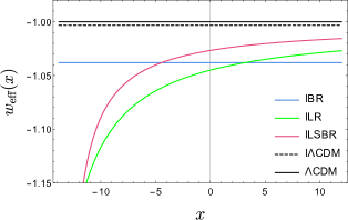
Figure 5: This figure shows the evolution of the effective EoS i.e. $w_{\textrm{eff}}=w_{\textrm{d}}-Q/3H\rho$ of $\Lambda$CDM, I$\Lambda$CDM, IBR, ILR and ILSBR models with respest to $x=\ln(a)$. The black vertical line denotes the present. We remind that $x=\ln(a)$ and $a=1$; i.e. $x=0$, at present.

We bring to the attention of the reader that in the case of a constant EoS i.e. $w_{\textrm{d}}=const$, one has to choose the coupling strength $\lambda$ and the EoS carefully. In Valiviita:2008iv ; Clemson:2011an ; Gavela:2010tm , the authors pointed out that for $w_{\textrm{d}}$CDM model, the interaction strength $\lambda$ and the quantity (1+$w_{\textrm{d}}$) must have the same signs for $Q\propto\rho_{d}$. A positive coupling is favoured by observations. Thus, our results are in agreement with Clemson:2011an ; Gavela:2009cy ; Gavela:2010tm ; Salvatelli:2013wra . In addition, models that are the object of this study have a phantom behaviour. This combination could give rise to some instabilities at the perturbative level. Even though, fitting observationally the cosmological perturbations is not the purpose of this paper, a perturbative analysis is considered qualitatively in order to compare the models under study and determine which model is the most favoured by observations.

VI PERTURBATIONS

In this section, we present a brief summary of the analysis of the linear cosmological perturbations of our interacting DE models. To this aim, we consider only scalar perturbations and the perturbed metric reads in the conformal time as

$$ds^{2}=a^{2} \left\{-\left(1+2\Phi\right)d\eta^{2}\right.$$

$$\left.+\left[\left(1-2\Psi\right)\delta_{ij}\right]dx^{i}dx^{j}\right\},$$ (34)

where $\eta$ is the conformal time, i.e. $d\eta=dt/a$. From now on, a prime will denote the derivative with respect to this conformal time. The physical quantities $\Phi$ and $\Psi$ are known as the Bardeen potentials. In the next step, we adopt the longitudinal (Newtonian) gauge, as can be seen by (VI) and we assume that none of the A-fluid introduces anisotropies at the linear perturbative level, i.e. the anisotropic stress $\pi_{A}=0$, which leads to the metric potentials equality $\Phi=\Psi$. Hence, the evolution equations of the dimensionless density perturbation $\delta_{A}=\delta\rho_{A}/\rho_{A}$ and the velocity perturbation $\theta_{A}$ are given by Valiviita:2008iv

$$\delta^{\prime}_{A}+3\mathcal{H}(c^{2}_{sA}-w_{\textrm{A}})\delta_{A}+(1+w_{\textrm{A}})\theta_{A}$$ (35)

$$+3\mathcal{H}[3\mathcal{H}(1+w_{\textrm{A}})(c^{2}_{sA}-c^{2}_{aA})]\frac{\theta_{A}}{k^{2}}-3(1+w_{\textrm{A}})\Psi^{\prime}$$

$$=\frac{aQ_{A}}{\rho_{A}}\left[\Psi-\delta_{A}+3\mathcal{H}(c^{2}_{sA}-c^{2}_{aA})\frac{\theta_{A}}{k^{2}}\right]+\frac{a}{\rho_{A}}\delta Q_{A},$$

$$\theta^{\prime}_{A}+\mathcal{H}(1-3c^{2}_{sA})\theta_{A}-\frac{c^{2}_{sA}}{\left(1+w_{\textrm{A}}\right)}k^{2}\delta_{A}-k^{2}\Psi$$ (36)

$$=\frac{aQ_{A}}{(1+w_{\textrm{A}})\rho_{A}}\left[\theta-(1+c^{2}_{sA})\theta_{A}\right]-\frac{a}{(1+w_{\textrm{A}})\rho_{A}}k^{2}f_{A}\hskip 2.84544pt,$$

where $A$ stands for radiation, CDM or DE fluid. The parameter $f_{A}$ describes the intrinsic momentum transfer of the fluid A and $c^{2}_{sA}$ is the sound speed in the A-fluid rest frame (r.f) defined as

$$\left.c_{sA}^{2}\equiv\frac{\delta p_{A}}{\delta\rho_{A}}\right|_{\textrm{r.f}}.$$ (37)

In the case of barotropic fluids $p_{A}(\rho_{A})$, the A-fluid speed of sound, $\frac{\delta p_{A}}{\delta\rho_{A}}$, coincides with the A-fluid adiabatic speed of sound, $c_{a\textrm{A}}^{2}$, which in the case of time varying EoS is defined as follows:

$$c_{a\textrm{A}}^{2}\equiv\frac{p^{\prime}_{A}}{\rho^{\prime}_{A}}=w_{\textrm{A}}+\frac{w_{\textrm{A}}^{\prime}\rho_{A}}{\rho_{\textrm{A}}^{\prime}}.$$ (38)

That is, barotropic fluids are completely adiabatic. Nevertheless, when dealing with DE fluids, given that $c^{2}_{\textrm{ad}}<0$ instabilities are induced at the perturbation level Gordon:2004ez . Therefore, in order to avoid those instabilities, it is convenient to consider a non adiabatic contribution on the DE pressure perturbation Bean:2003fb ; Valiviita:2008iv ,

$$\delta p_{\textrm{d},non-adiabatic}=\left(c^{2}_{s\textrm{d}}-c^{2}_{a\textrm{d}}\right)\delta\rho_{\textrm{d}}|_{\textrm{r.f}}\ ,$$ (39)

where the DE rest-frame speed of sound parameter, $c^{2}_{s\textrm{d}}$, it is a free parameter within the interval $[0,1]$ while the DE adiabatic speed of sound parameter, $c^{2}_{a\textrm{d}}$, could be time dependent.

The continuity equations can be rewritten as

$$\left\{\begin{array}[]{l}\dot{\rho}_{\textrm{m}}+3H\rho_{\textrm{m}}=Q_{\textrm{m}}\\ \dot{\rho}_{\textrm{d}}+3H(\rho_{\textrm{d}}+p_{\textrm{d}})=Q_{\textrm{d}},\end{array}\right.$$ (40)

where

$$aQ_{\textrm{d}}=-aQ_{\textrm{m}}=aQ=\lambda\mathcal{H}\rho_{\textrm{d}}\hskip 5.69046pt\textrm{and}\hskip 5.69046ptaQ_{\textrm{r}}=0.$$ (41)

The perturbation of the interaction term Q is given by

$$\delta Q=Q\left[\frac{\delta H}{H}+\delta_{\textrm{d}}\right],$$ (42)

note that, when the interaction term is proportional to $H$, i.e. $Q\propto H$, we must deal with the perturbation Hubble rate in order to get gauge invariant equations for the dark sector coupled models. The expression of the perturbation of $H$ in the longitudinal gauge is written as Gavela:2010tm

$$\frac{\delta H}{H}\equiv\frac{1}{\mathcal{H}}\left[\frac{\theta}{3}-\mathcal{H}\Psi-\Psi^{\prime}\right],$$ (43)

where $\theta$ is the volume expansion rate given by the partial contributions of each A-fluid

$$\theta=\sum_{A}\frac{1+w_{A}}{1+w}\Omega_{A}\theta_{A},\qquad\textrm{where}\qquad w=\sum_{A}\Omega_{A}w_{A}.$$ (44)

Finally, we can write the perturbation of the interaction term $Q=\lambda H\rho_{\textrm{d}}$ as

$$a\delta Q_{\textrm{m}} =-a\delta Q_{\textrm{d}}$$

$$=-\lambda\mathcal{H}\rho_{\textrm{d}}\left[\frac{\theta}{3\mathcal{H}}-\Psi-\frac{\Psi^{\prime}}{\mathcal{H}}+\delta_{d}\right],$$ (45)

In order to evaluate the growth rate, i.e. $f\sigma_{8}$, for the models under consideration we rewrite Eqs. (35) and (36) as follow Albarran:2016mdu :

$$\left(\delta_{\textrm{r}}\right)_{x} =\frac{4}{3}\left(\frac{k^{2}}{\mathcal{H}}v_{\textrm{r}}+3\Psi_{x}\right),$$ (46a)

$$\left(v_{\textrm{r}}\right)_{x} =-\frac{1}{\mathcal{H}}\left(\frac{1}{4}\delta_{\textrm{r}}+\Psi\right),$$ (46b)

$$\left(\delta_{\textrm{m}}\right)_{x} =\left(\frac{k^{2}}{\mathcal{H}}v_{\textrm{m}}+3\Psi_{x}\right)$$

$$+\frac{\lambda\rho_{\textrm{d}}}{\rho_{\textrm{m}}}\left[\frac{k^{2}v}{3\mathcal{H}}+\Psi_{x}-\delta_{\textrm{d}}+\delta_{\textrm{m}}\right],$$ (46c)

$$\left(v_{\textrm{m}}\right)_{x} =-\left(v_{\textrm{m}}+\frac{\Psi}{\mathcal{H}}\right),$$ (46d)

$$\left(\delta_{\textrm{d}}\right)_{x} =\left(1+w_{\textrm{d}}\right)\left\{\left[\frac{k^{2}}{\mathcal{H}}+9\mathcal{H}(c_{s\textrm{d}}^{2}-c_{a\textrm{d}}^{2})\right]v_{\textrm{d}}+3\Psi_{x}\right\}$$

$$+3\left(w_{\textrm{d}}-c_{s\textrm{d}}^{2}\right)\delta_{\textrm{d}}$$

$$-\lambda\left(\frac{k^{2}v}{3\mathcal{H}}+\Psi_{x}+3\mathcal{H}(c_{s\textrm{d}}^{2}-c_{a\textrm{d}}^{2})v_{\textrm{d}}\right),$$ (46e)

$$\left(v_{\textrm{d}}\right)_{x} =-\frac{1}{\mathcal{H}}\left(\frac{c_{s\textrm{d}}^{2}}{1+w_{\textrm{d}}}\delta_{\textrm{d}}+\Psi\right)+(3c_{s\textrm{d}}^{2}-1)v_{\textrm{d}}$$

$$+\frac{\lambda}{1+w_{\textrm{d}}}(v_{\textrm{m}}-(1+c_{s\textrm{d}}^{2})v_{\textrm{d}}),$$ (46f)

where $v$ is the total velocity potential related to $\theta$ as

$$v=-\frac{\theta}{k^{2}},$$ (47)

$x=\ln a$ and $(\;)_{x}$ is the derivative with respect to $x$. We have also used $(\;)^{\prime}=\mathcal{H}(\;)_{x}$ and $\theta_{A}=-k^{2}v_{A}$. In this work, we assume $c^{2}_{s\textrm{d}}=1$ as it is the case in the scalar field representation Bean:2003fb ; Valiviita:2008iv . In addition, we have chosen the momentum transfer parallel to the four velocity of DM, i.e. $f_{A}=Q_{A}\left(v_{\textrm{m}}-v\right)$, in such a way that the momentum transfer vanishes on the rest frame of DM Li:2013bya .

VI.1 Growth rate

In this section, we analyse the growth rate theoretical predictions i.e. $f\sigma_{8}$ of each studied model. These predictions will be then confronted to the observational data. To this aim, two compilations are used, namely RSD-63 which contains 63 data points published since 2006 until 2018 and the RSD-22 data which is the most robust 22 data compilation considered by the authors of Sagredo:2018ahx after analysing combinations of subsets in RSD-63 data points.

The evolution of these theoretical curves depend strongly on the best fit parameters deduced from the background analysis. The minimised $\chi^{2}_{f\sigma_{8}}$ of the growth rate is given by

$$\chi^{2}_{f\sigma_{8}}=\sum_{i=1}^{N}\left(\frac{f\sigma_{8,th}(z_{i})-f\sigma_{8}(z_{i})}{\sigma_{f\sigma_{8}}}\right)^{2},$$ (48)

where $N=63$ $(22)$ for RSD-63 (RSD-22) data.

	$\chi^{2}_{f\sigma_{8}}$
Model	$\bf RSD22$	$\bf RSD63$
$\Lambda$CDM	0.8181	0.7762
I$\Lambda$CDM	0.9993	0.9045
IBR	1.1439	1.0236
ILR	1.1713	1.0485
ILSBR	1.1208	1.00343

Table 4: This table presents the reduced $\chi^{2}_{f\sigma_{8}}$ values of the perturbative analysis. These results are obtained after the confrontation of models with the growth dataset RSD-63 and RSD-22 shown in table 5.

Table 4, shows the reduced $\chi^{2}_{f\sigma_{8}}$ values for all models studied. The reduced $\chi^{2}$ is a powerful tool to test the goodness of fit, it takes into account, the minimal value of $\chi^{2}$, the number of free parameters and the total number of data points. If we compare models, the best one is that whose $\chi^{2}_{red}$ value is closest to 1. $\Lambda$CDM model presents an over fit for both RSD-22 and RSD-63 data. Indeed, this conclusion is due to the injection of the best fit parameters extracted from the background statistics in $\chi^{2}_{f\sigma_{8}}$. These results are viewed as a qualitative since they depend strongly on the background analysis. The interacting model I$\Lambda$CDM shows a better fit of both RSD-22 and RSD-63 than $\Lambda$CDM. It seems also that the RSD-63 data fit the interacting models, IBR, ILR and ILBR better than RSD-22 data does.

Index	$z$	$f\sigma_{8}$	Survey	Ref.	Year
1	0.02	$0.314\phantom{}\pm 0.048\phantom{}$	2MASS	Davis:2010sw	13 November 2010
2	0.02	$0.398\phantom{}\pm 0.065\phantom{}$	SNIa + IRAS	Turnbull:2011ty	20 October 2011
3	0.02	$0.428\phantom{}\pm 0.046\phantom{}$	6dF Galaxy Survey + SNIa	Huterer:2016uyq	29 November 2016
4	0.10	$0.370\phantom{}\pm 0.130\phantom{}$	SDSS-veloc	Feix:2015dla	16 June 2015
5	0.15	$0.490\phantom{0}\pm 0.145\phantom{0}$	SDSS DR7 MGS	Howlett:2014opa	30 January 2015
6	0.17	$0.510\phantom{0}\pm 0.060\phantom{0}$	2dF Galaxy Redshift Survey	Percival:2004fs ; Song:2008qt	6 October 2009
7	0.18	$0.360\phantom{}\pm 0.090\phantom{}$	GAMA	Blake:2013nif	22 September 2013
8	0.25	$0.3512\pm 0.0583$	SDSS II LRG	Samushia:2011cs	9 December 2011
9	0.32	$0.384\pm 0.095$	BOSS-LOWZ	Sanchez:2013tga	17 December 2013
10	0.37	$0.4602\pm 0.0378$	SDSS II LRG	Samushia:2011cs	9 December 2011
11	0.38	$0.440\pm 0.060$	GAMA	Blake:2013nif	22 September 2013
12	0.44	$0.413\pm 0.080$	WiggleZ Dark Energy Survey + Alcock-Paczynski distortion	Blake:2012pj	12 June 2012
13	0.59	$0.488\pm 0.06\phantom{0}$	SDSS III BOSS DR12 CMASS	Chuang:2013wga	8 June 2016
14	0.60	$0.390\pm 0.063$	WiggleZ Dark Energy Survey + Alcock-Paczynski distortion	Blake:2012pj	12 June 2012
15	0.60	$0.550\pm 0.120$	Vipers PDR-2	Pezzotta:2016gbo	16 Decembre 2016
16	0.73	$0.437\pm 0.072$	WiggleZ Dark Energy Survey + Alcock-Paczynski distortion	Blake:2012pj	12 June 2012
17	0.86	$0.400\pm 0.110\phantom{}$	Vipers PDR-2	Pezzotta:2016gbo	16 Decembre 2016
18	0.978	$0.379\pm 0.0.176$	SDSS-IV	Okada:2015vfa	9 January 2018
19	1.23	$0.385\pm 0.099$	SDSS-IV	Okada:2015vfa	9 January 2018
20	1.40	$0.482\pm 0.116$	FastSound	Okada:2015vfa	25 November 2015
21	1.526	$0.342\pm 0.070$	SDSS-IV	Okada:2015vfa	9 January 2018
22	1.944	$0.364\pm 0.106$	SDSS-IV	Okada:2015vfa	9 January 2018
23	0.35	$0.44\pm 0.05$	SDSS-LRG	Okada:2015vfa	30 October 2006
24	0.77	$0.490\pm 0.18$	VVDS	Okada:2015vfa	6 October 2009
25	0.25	$0.3665\pm 0.0601$	SDSS-LRG-60	Okada:2015vfa	9 December 2011
26	0.37	$0.4031\pm 0.0586$	SDSS-LRG-60	Okada:2015vfa	9 December 2011
27	0.067	$0.423\pm 0.055$	6dFGS	Okada:2015vfa	4 July 2012
28	0.30	$0.407\pm 0.055$	SDSS-BOSS	Okada:2015vfa	11 August 2012
29	0.40	$0.419\pm 0.041$	SDSS-BOSS	Okada:2015vfa	11 August 2012
30	0.50	$0.427\pm 0.043$	SDSS-BOSS	Okada:2015vfa	11 August 2012
31	0.60	$0.433\pm 0.067$	SDSS-BOSS	Okada:2015vfa	11 August 2012
32	0.80	$0.47\pm 0.08$	Vipers	Okada:2015vfa	9 July 2013
33	0.35	$0.429\pm 0.089$	SDSS-DR7-LRG	Okada:2015vfa	8 August 2013
34	0.32	$0.48\pm 0.1$	SDSS DR10 and DR11	Okada:2015vfa	17 December 2013
35	0.57	$0.417\pm 0.045$	SDSS DR10 and DR11	Okada:2015vfa	17 December 2013
36	0.38	$0.497\pm 0.045$	BOSS DR12	Okada:2015vfa	11 July 2016
37	0.51	$0.458\pm 0.038$	BOSS DR12	Okada:2015vfa	11 July 2016
38	0.61	$0.436\pm 0.034$	BOSS DR12	Okada:2015vfa	11 July 2016
39	0.38	$0.477\pm 0.051$	BOSS DR12	Okada:2015vfa	11 July 2016
40	0.51	$0.453\pm 0.05$	BOSS DR12	Okada:2015vfa	11 July 2016
41	0.61	$0.410\pm 0.044$	BOSS DR12	Okada:2015vfa	11 July 2016
42	0.76	$0.440\pm 0.040$	Vipers v7	Okada:2015vfa	26 October 2016
43	1.05	$0.280\pm 0.080$	Vipers v7	Okada:2015vfa	26 October 2016
44	0.32	$0.427\pm 0.056$	BOSS-LOWZ	Okada:2015vfa	26 October 2016
45	0.57	$0.426\pm 0.029$	BOSS CMASS	Okada:2015vfa	26 October 2016
46	0.727	$0.296\pm 0.0765$	Vipers	Okada:2015vfa	21 November 2016
47	0.6	$0.48\pm 0.12$	Vipers	Okada:2015vfa	16 December 2016
48	0.86	$0.48\pm 0.1$	Vipers	Okada:2015vfa	16 December 2016
49	0.1	$0.480\pm 0.16$	SDSS DR13	Okada:2015vfa	22 December 2016
50	0.001	$0.505\pm 0.085$	2MTF	Okada:2015vfa	16 June 2017
51	0.85	$0.45\pm 0.11$	Vipers PDR-2	Okada:2015vfa	31 July 2017
52	0.31	$0.469\pm 0.098$	BOSS DR12	Okada:2015vfa	15 September 2017
53	0.36	$0.474\pm 0.097$	BOSS DR12	Okada:2015vfa	15 September 2017
54	0.4	$0.473\pm 0.086$	BOSS DR12	Okada:2015vfa	15 September 2017
55	0.44	$0.481\pm 0.076$	BOSS DR12	Okada:2015vfa	15 September 2017
56	0.48	$0.482\pm 0.067$	BOSS DR12	Okada:2015vfa	15 September 2017
57	0.52	$0.488\pm 0.065$	BOSS DR12	Okada:2015vfa	15 September 2017
58	0.56	$0.482\pm 0.067$	BOSS DR12	Okada:2015vfa	15 September 2017
59	0.59	$0.481\pm 0.066$	BOSS DR12	Okada:2015vfa	15 September 2017
60	0.64	$0.486\pm 0.07$	BOSS DR12	Okada:2015vfa	15 September 2017
61	0.1	$0.376\pm 0.038$	SDSS DR7	Okada:2015vfa	12 December 2017
62	1.52	$0.42\pm 0.076$	SDSS-IV	Okada:2015vfa	8 Junuary 2018
63	1.52	$0.396\pm 0.079$	SDSS-IV	Okada:2015vfa	8 Junuary 2018

Table 5: This table shows a compilation of $f\sigma_{8}$ redshift space distortion (RSD) data, published since 2006 until 2018.

VII CONCLUSION

The purpose of the current paper is to study the behaviour of three interacting phantom dark energy models, labeled as IBR, ILR and ILSBR, where the dark components interact with each other, via a non gravitational interaction. We consider an interaction between DE and CDM densities to find out its impact on the cosmological parameters i.e. $\Omega_{m}$, $\Omega_{d}$ and $h$, as well as, to find out its impact on the persistence or the dissapearance of singularities and abrupt events. We have considered an interaction of the form $Q=\lambda H\rho_{\textrm{d}}$, because it does not give rise to a large scale instability at early times with $\lambda>0$ Li:2013bya . We have studied models at the background level as well as at the perturbative level. The background study consists in confronting the theoretical predictions of the models with the joined observational data corresponding to supernova from Pantheon, CMB from Planck 2018, BAO from (SDSS DR12, SDSS MGS, WiggleZ, 6dFGS, Lya, DES) and $H(z)$ by means of an MCMC approach, which allowed us to extracted the best fit parameters as well as their corresponding minimal chi squared values. In order to classify these models, we have used the $\textrm{AIC}_{c}$ tool. The results of the background statistical analysis reported that $\Lambda$CDM is always the best model, followed by I$\Lambda$CDM, ILR, ILSBR, and IBR. We remark that the interaction has changed the order of the preferred model in Bouali:2019whr . As can be seen in table 2, observations favour a positive interaction for all models i.e. CDM decays into DE. We observe also that for IBR, ILR and ILSBR, the amount of the CDM energy density transformed to DE density is of order $10^{-2}$, while for I$\Lambda$CDM the amount of CDM density transformed into DE density is of the order $10^{-3}$. Unfortunately, this process exacerbates the energy density transfer from CDM into DE in the future, as shown in figure 4, by giving rise to a non physical results which breaks down the validity of this interaction in the future. From the MCMC approach, we have constrained the cosmological parameters of each phantom models. Table 2 summarizes the best fit parameters of these models. By using the best fit parameters of the background analysis, we have solved numerically the perturbation equations system which allowed us to confront the predicted $f\sigma_{8}$ of each model to observations i.e. RSD-22 and RSD-63. It was shown that the theoretical curves of IBR, ILR and ILSBR fit better the RSD-63 compilation. It seems that $\Lambda$CDM and I$\Lambda$CDM over fit both RDS-22 and RSD-63 compilations. Both RSD compilations reported that the classification of preferred models according to observations is as follows: $\Lambda$CDM, I$\Lambda$CDM, ILSBR, IBR and ILR model. In fact the perturbation results are not conclusive since they depend strongly on the background results. Consequently, our perturbative results can be seen as qualitative. However, notice that our models are consistent with RSD compilations.

Cosmological observations show that the singularity induced by the BR model as well as the abrupt events corresponding to the LR and the LSBR remain, even when the dark components interact with each other at least for the interaction we have chosen.

VIII ACKNOWLEDGMENTS

The work of M.B.L. is supported by the Basque Foundation of Science Ikerbasque. She also would like to acknowledge the support from the Basque government Grant No. IT956- 16 (Spain) and from the Grant PID2020-114035GB-100 funded by MCIN/AEI/10.13039/501100011033 and by “ERDF A way of making Europe”.

References

- (1) A. G. Riess et al. [Supernova Search Team Collaboration], Astron. J. 116 (1998) 1009 [astro-ph/9805201].
- (2) S. Perlmutter et al. [Supernova Cosmology Project Collaboration], Astrophys. J. 517 (1999) 565 [astro-ph/9812133].
- (3) P. A. R. Ade et al. [Planck Collaboration], Astron. Astrophys. 594 (2016) A14 [arXiv:1502.01590 [astro-ph.CO]].
- (4) R. G. Cai and A. Wang, JCAP 0503 (2005) 002 [[hep-th/0411025]].
- (5) I. Duran and D. Pavón, Phys. Rev. D 83 (2011) 023504 [[arXiv:1012.2986 [astro-ph.CO]]].
- (6) B. Ratra and P. J. E. Peebles, [Phys. Rev. D 37 (1988) 3406.
- (7) C. Armendariz-Picon, V. F. Mukhanov and P. J. Steinhardt, Phys. Rev. D 63 (2001) 103510 [[astro-ph/0006373]].
- (8) A. Y. Kamenshchik, U. Moschella and V. Pasquier, Phys. Lett. B 511 (2001) 265 doi:10.1016/S0370-2693(01)00571-8 [gr-qc/0103004].
- (9) T. P. Sotiriou and V. Faraoni, Rev. Mod. Phys. 82 (2010) 451 [ [arXiv:0805.1726 [gr-qc]]].
- (10) A. De Felice and S. Tsujikawa, Living Rev. Rel. 13 (2010) 3 [arXiv:1002.4928 [gr-qc]]].
- (11) R. Ferraro and F. Fiorini, Phys. Rev. D 75 (2007) 084031 [[gr-qc/0610067]].
- (12) R. Ferraro and F. Fiorini, Phys. Rev. D 78 (2008) 124019 [[arXiv:0812.1981 [gr-qc]]].
- (13) G. R. Bengochea and R. Ferraro, Phys. Rev. D 79 (2009) 124019 [[arXiv:0812.1205 [astro-ph]]].
- (14) T. Harko, F. S. N. Lobo, S. Nojiri and S. D. Odintsov, Phys. Rev. D 84 (2011) 024020 [[arXiv:1104.2669 [gr-qc]]].
- (15) S. Nojiri and S. D. Odintsov, Phys. Lett. B 599 (2004), 137-142 [[arXiv:astro-ph/0403622 [astro-ph]]].
- (16) G. Allemandi, A. Borowiec, M. Francaviglia and S. D. Odintsov, Phys. Rev. D 72 (2005), 063505 [[arXiv:gr-qc/0504057 [gr-qc]]].
- (17) S. Nojiri and S. D. Odintsov, Phys. Rev. D 74 (2006), 086005 [[arXiv:hep-th/0608008 [hep-th]]].
- (18) S. Nojiri, S. D. Odintsov and D. Saez-Gomez, Phys. Lett. B 681 (2009), 74-80 [[arXiv:0908.1269 [hep-th]]].
- (19) N. Aghanim et al. [Planck Collaboration], Astron. Astrophys. 641 (2020) A6 [[arXiv:1807.06209 [astro-ph.CO]]].
- (20) R. R. Caldwell, Phys. Lett. B 545 (2002) 23 [astro-ph/9908168].
- (21) J. Beltrán Jiménez, R. Lazkoz, D. Sáez-Gómez and V. Salzano, Eur. Phys. J. C 76 (2016) no.11, 631 [arXiv:1602.06211 [gr-qc]].
- (22) V. Sahni, A. Shafieloo and A. A. Starobinsky, Astrophys. J. 793 (2014) no.2, L40 [arXiv:1406.2209 [astro-ph.CO]].
- (23) S. Vagnozzi, S. Dhawan, M. Gerbino, K. Freese, A. Goobar and O. Mena, Phys. Rev. D 98 (2018) no.8, 083501 [arXiv:1801.08553 [astro-ph.CO]].
- (24) U. Alam, S. Bag and V. Sahni, Phys. Rev. D 95 (2017) no.2, 023524 [arXiv:1605.04707 [astro-ph.CO]].
- (25) M. P. Da̧browski, T. Stachowiak, and M. Szydłowski, Phys. Rev. D 68 (2003) 103519 [hep-th/0307128].
- (26) A. A. Starobinsky, Grav. Cosmol. 6 (2000) 157 [astro-ph/9912054].
- (27) R. R. Caldwell, M. Kamionkowski and N. N. Weinberg, Phys. Rev. Lett. 91 (2003) 071301 [astro-ph/0302506].
- (28) S. M. Carroll, M. Hoffman and M. Trodden, Phys. Rev. D 68 (2003) 023509 [astro-ph/0301273].
- (29) L. P. Chimento and R. Lazkoz, Phys. Rev. Lett. 91 (2003) 211301 [gr-qc/0307111].
- (30) P. F. González-Díaz, Phys. Lett. B 586 (2004) 1 [astro-ph/0312579].
- (31) P. F. González-Díaz, Phys. Rev. D 69 (2004) 063522 [hep-th/0401082].
- (32) V. Sahni and Y. Shtanov, JCAP 0311 (2003) 014 [[astro-ph/0202346]].
- (33) T. Ruzmaikina and A. A. Ruzmaikin, Sov. Phys. JETP 30 (1970) 372.
- (34) H. Štefančić, Phys. Rev. D 71 (2005) 084024 [astro-ph/0411630].
- (35) S. ’i. Nojiri, S. D. Odintsov and S. Tsujikawa, Phys. Rev. D 71 (2005) 063004 [hep-th/0501025].
- (36) S. ’i. Nojiri and S. D. Odintsov, Phys. Rev. D 72 (2005) 023003 [hep-th/0505215].
- (37) M. Bouhmadi-López, Nucl. Phys. B 797 (2008) 78 [astro-ph/0512124].
- (38) P. H. Frampton, K. J. Ludwick and R. J. Scherrer, Phys. Rev. D 84 (2011) 063003 [arXiv:1106.4996 [astro-ph.CO]].
- (39) I. Brevik, E. Elizalde, S. ’i. Nojiri, and S. D. Odintsov, Phys. Rev. D 84 (2011) 103508 [arXiv:1107.4642 [hep-th]].
- (40) M. Bouhmadi-López, P. Chen, and Y. W. Liu, Eur. Phys. J. C 73 (2013) 2546 [arXiv:1302.6249 [gr-qc]].
- (41) F. Contreras, N. Cruz, E. Elizalde, E. González and S. Odintsov, Phys. Rev. D 98 (2018) no.12, 123520 [arXiv:1808.06546 [gr-qc]].
- (42) M. Bouhmadi-López, A. Errahmani, P. Martín-Moruno, T. Ouali, and Y. Tavakoli, Int. J. Mod. Phys. D 24 (2015) no.10, 1550078 [arXiv:1407.2446 [gr-qc]].
- (43) J. Morais, M. Bouhmadi-López, K. Sravan Kumar, J. Marto and Y. Tavakoli, Phys. Dark Univ. 15 (2017) 7 [arXiv:1608.01679 [gr-qc]].
- (44) M. Bouhmadi-López, D. Brizuela and I. Garay, JCAP 1809 (2018) no.09, 031 [ [arXiv:1802.05164 [gr-qc]]].
- (45) I. Albarran, M. Bouhmadi-López and J. Morais, Phys. Dark Univ. 16 (2017) 94 [[arXiv:1611.00392 [astro-ph.CO]]].
- (46) A. Bouali, I. Albarran, M. Bouhmadi-López and T. Ouali, Phys. Dark Univ. 26 (2019) 100391 [[arXiv:1905.07304 [astro-ph.CO]]].
- (47) B. Sagredo, S. Nesseris and D. Sapone, Phys. Rev. D 98 (2018) no.8, 083543 [[arXiv:1806.10822 [astro-ph.CO]]].
- (48) L. Amendola, Phys. Rev. D 60 (1999) 043501 [[astro-ph/9904120]].
- (49) A. P. Billyard and A. A. Coley, Phys. Rev. D 61 (2000) 083503 [[astro-ph/9908224]].
- (50) W. Zimdahl and D. Pavón, Phys. Lett. B 521 (2001) 133 [[astro-ph/0105479]].
- (51) G. R. Farrar and P. J. E. Peebles, Astrophys. J. 604 (2004) 1 µdoi:10.1086/381728 [[astro-ph/0307316]].
- (52) L. P. Chimento, A. S. Jakubi, D. Pavón and W. Zimdahl, Phys. Rev. D 67 (2003) 083513 [[astro-ph/0303145]].
- (53) G. Olivares, F. Atrio-Barandela and D. Pavón, Phys. Rev. D 71 (2005) 063523 [[astro-ph/0503242]].
- (54) T. Koivisto, Phys. Rev. D 72 (2005) 043516 [[astro-ph/0504571]].
- (55) H. M. Sadjadi and M. Alimohammadi, Phys. Rev. D 74 (2006) 103007 [[gr-qc/0610080]].
- (56) Z. K. Guo, N. Ohta and S. Tsujikawa, Phys. Rev. D 76 (2007) 023508 [[astro-ph/0702015 [ASTRO-PH]]].
- (57) J. Zhang, H. Liu and X. Zhang, Phys. Lett. B 659 (2008) 26 [[arXiv:0705.4145 [astro-ph]]].
- (58) C. G. Boehmer, G. Caldera-Cabral, R. Lazkoz and R. Maartens, Phys. Rev. D 78 (2008) 023505 [[arXiv:0801.1565 [gr-qc]]].
- (59) S. H. Pereira and J. F. Jesus, Phys. Rev. D 79 (2009) 043517 [[arXiv:0811.0099 [astro-ph]]].
- (60) J. H. He, B. Wang, E. Abdalla and D. Pavón, JCAP 1012 (2010) 022 [[arXiv:1001.0079 [gr-qc]]].
- (61) Y. H. Li and X. Zhang, Eur. Phys. J. C 71 (2011) 1700 [[arXiv:1103.3185 [astro-ph.CO]]].
- (62) T. Clemson, K. Koyama, G. B. Zhao, R. Maartens and J. Valiviita, Phys. Rev. D 85 (2012) 043007 [[arXiv:1109.6234 [astro-ph.CO]]].
- (63) X. D. Xu, B. Wang, P. Zhang and F. Atrio-Barandela, JCAP 1312 (2013) 001 [[arXiv:1308.1475 [astro-ph.CO]]].
- (64) G. Cheng, Y. Z. Ma, F. Wu, J. Zhang and X. Chen, Phys. Rev. D 102 (2020) no.4, 043517 [[arXiv:1911.04520 [astro-ph.CO]]].
- (65) M. Bouhmadi-López, A. Errahmani, T. Ouali and Y. Tavakoli, Eur. Phys. J. C, 78 (2018) 330, [arXiv:1707.07200].
- (66) M-H. Belkacemi, Z. Bouabdallaoui, M. Bouhmadi-López, A. Errahmani and T. Ouali, IJMP D29, N9 (2020)2050066, [arXiv:1812.06782v3].
- (67) D. M. Scolnic et al., Astrophys. J. 859 (2018) no.2, 101 [arXiv:1710.00845 [astro-ph.CO]].
- (68) Z. Zhai and Y. Wang, JCAP 1907 (2019) no.07, 005 [arXiv:1811.07425 [astro-ph.CO]].
- (69) L. Anderson et al. [BOSS Collaboration], Mon. Not. Roy. Astron. Soc. 441 (2014) no.1, 24 [arXiv:1312.4877 [astro-ph.CO]].
- (70) F. Beutler et al., Mon. Not. Roy. Astron. Soc. 416 (2011) 3017 [arXiv:1106.3366 [astro-ph.CO]].
- (71) A. J. Ross, L. Samushia, C. Howlett, W. J. Percival, A. Burden and M. Manera, Mon. Not. Roy. Astron. Soc. 449 (2015) no.1, 835 [arXiv:1409.3242 [astro-ph.CO]].
- (72) E. A. Kazin et al., Mon. Not. Roy. Astron. Soc. 441 (2014) no.4, 3524 [arXiv:1401.0358 [astro-ph.CO]].
- (73) S. Alam et al. [BOSS Collaboration], Mon. Not. Roy. Astron. Soc. 470 (2017) no.3, 2617 [arXiv:1607.03155 [astro-ph.CO]].
- (74) C. Zhang, H. Zhang, S. Yuan, T. J. Zhang and Y. C. Sun, Res. Astron. Astrophys. 14 (2014) no.10, 1221 [arXiv:1207.4541 [astro-ph.CO]].
- (75) D. Stern, R. Jimenez, L. Verde, M. Kamionkowski and S. A. Stanford, JCAP 1002 (2010) 008 [arXiv:0907.3149 [astro-ph.CO]].
- (76) M. Moresco et al., JCAP 1208 (2012) 006 [arXiv:1201.3609 [astro-ph.CO]].
- (77) C. H. Chuang and Y. Wang, Mon. Not. Roy. Astron. Soc. 435 (2013) 255 [arXiv:1209.0210 [astro-ph.CO]].
- (78) M. Moresco, Mon. Not. Roy. Astron. Soc. 450 (2015) no.1, L16 [arXiv:1503.01116 [astro-ph.CO]].
- (79) M. Moresco et al., JCAP 1605 (2016) no.05, 014 [arXiv:1601.01701 [astro-ph.CO]].
- (80) P. Stöcker, M. Krämer, J. Lesgourgues and V. Poulin, JCAP 1803 (2018) no.03, 018 [arXiv:1801.01871 [astro-ph.CO]].
- (81) M. Abramowitz and I. A. Stegun. Handbook of mathematical functions (Dover, 1980).
- (82) M. Bouhmadi-López, C. Kiefer and P. Martín-Moruno, arXiv:1904.01836 [gr-qc]. [arXiv:1904.01836 [gr-qc]].
- (83) A. G. Riess, S. Casertano, W. Yuan, L. M. Macri and D. Scolnic, Astrophys. J. 876 (2019) no.1, 85 [arXiv:1903.07603 [astro-ph.CO]].
- (84) E. Di Valentino, O. Mena, S. Pan, L. Visinelli, W. Yang, A. Melchiorri, D. F. Mota, A. G. Riess and J. Silk, Class. Quant. Grav. 38 (2021) no.15, 153001 [arXiv:2103.01183 [astro-ph.CO]].
- (85) H. Akaike, [https://ieeexplore.ieee.org/document/1100705].
- (86) J. Valiviita, E. Majerotto and R. Maartens, JCAP 0807 (2008) 020 [ [arXiv:0804.0232 [astro-ph]]].
- (87) M. B. Gavela, L. Lopez Honorez, O. Mena and S. Rigolin, JCAP 1011 (2010) 044 [[arXiv:1005.0295 [astro-ph.CO]]].
- (88) M. B. Gavela, D. Hernandez, L. Lopez Honorez, O. Mena and S. Rigolin, JCAP 0907 (2009) 034 Erratum: [JCAP 1005 (2010) E01] [[arXiv:0901.1611 [astro-ph.CO]]].
- (89) V. Salvatelli, A. Marchini, L. Lopez-Honorez and O. Mena, Phys. Rev. D 88 (2013) no.2, 023531 [[arXiv:1304.7119 [astro-ph.CO]]].
- (90) C. Gordon and W. Hu, Phys. Rev. D 70 (2004) 083003 doi:10.1103/PhysRevD.70.083003 [astro-ph/0406496].
- (91) R. Bean and O. Doré, Phys. Rev. D 69 (2004) 083503 [astro-ph/0307100].
- (92) Y. H. Li and X. Zhang, Phys. Rev. D 89 (2014) no.8, 083009 [[arXiv:1312.6328 [astro-ph.CO]]].
- (93) M. Davis, A. Nusser, K. Masters, C. Springob, J. P. Huchra and G. Lemson, Mon. Not. Roy. Astron. Soc. 413 (2011) 2906 [arXiv:1011.3114 [astro-ph.CO]].
- (94) S. J. Turnbull, M. J. Hudson, H. A. Feldman, M. Hicken, R. P. Kirshner and R. Watkins, Mon. Not. Roy. Astron. Soc. 420 (2012) 447 [arXiv:1111.0631 [astro-ph.CO]].
- (95) D. Huterer, D. Shafer, D. Scolnic and F. Schmidt, JCAP 1705 (2017) no.05, 015 [arXiv:1611.09862 [astro-ph.CO]].
- (96) M. Feix, A. Nusser and E. Branchini, Phys. Rev. Lett. 115 (2015) no.1, 011301 [arXiv:1503.05945 [astro-ph.CO]].
- (97) C. Howlett, A. Ross, L. Samushia, W. Percival and M. Manera, Mon. Not. Roy. Astron. Soc. 449 (2015) no.1, 848 [arXiv:1409.3238 [astro-ph.CO]].
- (98) W. J. Percival et al. [2dFGRS Collaboration], Mon. Not. Roy. Astron. Soc. 353 (2004) 1201 [astro-ph/0406513].
- (99) Y. S. Song and W. J. Percival, JCAP 0910 (2009) 004 [arXiv:0807.0810 [astro-ph]].
- (100) C. Blake et al., Mon. Not. Roy. Astron. Soc. 436 (2013) 3089 [[arXiv:1309.5556 [astro-ph.CO]]].
- (101) L. Samushia, W. J. Percival and A. Raccanelli, Mon. Not. Roy. Astron. Soc. 420 (2012) 2102 [arXiv:1102.1014 [astro-ph.CO]].
- (102) A. G. Sánchez et al., Mon. Not. Roy. Astron. Soc. 440 (2014) no.3, 2692 [arXiv:1312.4854 [astro-ph.CO]].
- (103) C. Blake et al., Mon. Not. Roy. Astron. Soc. 425 (2012) 405 [arXiv:1204.3674 [astro-ph.CO]].
- (104) C. H. Chuang et al., Mon. Not. Roy. Astron. Soc. 461 (2016) no.4, 3781 [arXiv:1312.4889 [astro-ph.CO]].
- (105) A. Pezzotta et al., Astron. Astrophys. 604 (2017) A33 [arXiv:1612.05645 [astro-ph.CO]].
- (106) H. Okada et al., Publ. Astron. Soc. Jap. 68 (2016) no.33, id.47, 17 [arXiv:1504.05592 [astro-ph.GA]].